Dynamics of the Wigner Crystal of Composite Particles

Abstract

Conventional wisdom had long held that a composite particle behaves just like an ordinary Newtonian particle. In this paper, we derive the effective dynamics of a type-I Wigner crystal of composite particles directly from its microscopic wave function. It indicates that the composite particles are subjected to a Berry curvature in the momentum space as well as an emergent dissipationless viscosity. Therefore, contrary to the general belief, composite particles follow the more general Sundaram-Niu dynamics instead of the ordinary Newtonian one. We show that the presence of the Berry curvature is an inevitable feature for a dynamics consistent with the dipole picture of composite particles and Kohn’s theorem. Based on the dynamics, we determine the dispersions of magneto-phonon excitations numerically. We find an emergent magneto-roton mode which signifies the composite-particle nature of the Wigner crystal. It occurs at frequencies much lower than the magnetic cyclotron frequency and has a vanishing oscillator strength in the long wavelength limit.

I Introduction

In a two-dimensional electron gas (2DEG) subjected to a strong magnetic field, electrons are forced into Landau levels with the kinetic energy quenched. The dominating electron-electron interaction induces various correlated ground states. The most celebrated of these states is the fractional quantum Hall (FQH) liquid which occurs in the vicinity of a set of magnetic filling factors of rational fractions Jainendra K. Jain (2007). Interestingly, even though the system is dominated by the electron-electron interaction, its physics can be well described in a hidden Hilbert space by a set of weakly interacting composite fermions (bosons) that are bound states of an electron with an even (odd) number of quantum vortices, as suggested by the theory of composite fermions (CFs) Jainendra K. Jain (2007); Jain and Anderson (2009). In the theory, a FQH state is interpreted as an integer quantum Hall state of CFs. The theory achieves great successes. For instance, the ground state wave functions prescribed by the CF theory for the FQH states achieve high overlaps with those determined from exact diagonalizations Jainendra K. Jain (2007), and the predictions based on an intuitive picture of non-interacting CFs are verified in various experiments O. Heinonen (1997). The theory can even be applied to more exotic situations such as the half-filling case which is interpreted as a Fermi liquid of CFs Kalmeyer and Zhang (1992); Halperin et al. (1993), and the $5/2$-filling case which is interpreted as a $p$-wave pairing state of CFs Moore and Read (1991). In effect, for every known state of electrons, one could envision a counterpart for CFs.

It is natural to envision that CFs may form a Wigner crystal (WC). Electrons form a Wigner crystal at sufficiently low density when the electron-electron interaction dominates over the kinetic energy Gabriele Giuliani and Giovanni Vignale (2005). In the presence of a strong external magnetic field, the kinetic energy is completely quenched and electrons should have a tendency to form a crystalline phase. However, in 2DEG, the tendency is preempted by the more stable FQH states when the filling factor is close to special fractions such as $1/3$ and $2/5$. Nevertheless, a WC could be stabilized when the filling factor deviates from these fractions. Theoretical studies suggest that the WC of composite particles (CPWC), i.e., a WC consisting not of electrons but composite fermions or bosons, could be stabilized Yi and Fertig (1998). More specifically, either a type-I CPWC Yi and Fertig (1998); Narevich et al. (2001), in which all composite particles (CPs) are frozen, or a type-II CPWC Archer et al. (2013), which lives on top of a FQH state and only freezes CFs excessive for the filling fraction of the FQH state, could be energetically favored over the ordinary electron WC Yi and Fertig (1998); Yang et al. (2001); Lee et al. (2002); Goerbig et al. (2004); Chang et al. (2005, 2006). Experimentally, there had accumulated a large number of evidences indicating the formations of WCs in 2DEG systems, although these experiments, either detecting the microwave resonances of disorder pinning modes Andrei et al. (1988); Engel et al. (1997); Li et al. (1997, 2000); Chen et al. (2003, 2004, 2006); Zhu et al. (2010); Williams et al. (1991) or measuring transport behaviors Zhang et al. (2015); Liu et al. (2014); Pan et al. (2002); Li et al. (1991); Jiang et al. (1991); Williams et al. (1991); Jiang et al. (1990); Goldman et al. (1990), cannot unambiguously distinguish a CPWC from its ordinary electron counterpart.

A possible way to distinguish a CPWC from its ordinary electron counterpart is to examine its low energy phonon excitation. The phonon excitation of an ordinary WC had been thoroughly investigated Maki and Zotos (1983); Côté and MacDonald (1990, 1991). It consists of a low-frequency branch and a magneto-plasmon mode that occurs near the magnetic cyclotron frequency. Moreover, Kohn’s theorem asserts that the magnetic cyclotron mode exhausts all the spectral weight in the long wavelength limit Kalmeyer and Zhang (1992); Simon (1998). For a CPWC, in analog to the ordinary WC, one would expect that its phonon excitation also consists of two branches. However, similar to the magneto-roton mode arisen in FQH liquids Girvin et al. (1986), its high-frequency branch must be an emergent mode originated purely from the electron-electron interaction, irrelevant to the cyclotron resonance because all excitations of CPs are limited within a partially filled Landau level. To be consistent with Kohn’s theorem, the mode must have a vanishing oscillator strength in the long wavelength limit. These features of the emergent mode make it unique. An experimental probe of the mode would provide an unambiguous evidence for the CP nature of an observed WC phase.

To determine the low-energy phonon excitation of a CPWC, it is necessary to understand the dynamics of CPs. Unfortunately, up to now, the true nature of the CP dynamics is yet to be fully clarified. Existing theories are based on a heuristic approach assuming that CPs follow the ordinary dynamics characterized by an effective mass and an effective magnetic field Rhim et al. (2015); Archer and Jain (2011); Ettouhami et al. (2006). The assumption is in accordance with the conventional wisdom that a CP behaves just like an ordinary Newtonian particle, as implied in either the Halperin-Lee-Read theory of composite Fermi-liquids Halperin et al. (1993) or López-Fradkin’s construction of the Chern-Simons field theory for FQH states Lopez and Fradkin (1991). However, the validity of the assumption is questionable. An indication of that is the violation of Kohn’s theorem: the heuristic approach would predict a new cyclotron mode corresponding to the effective mass and magnetic field. It hints that the CP dynamics adopted by the heuristic approach cannot be the correct one. Actually, even for electrons in a solid, the dynamics in general has a symplectic form (Sundaram-Niu dynamics) in which Berry curvature corrections emerge as a result of the coupling between orbital and internal degrees of freedom (e.g., spin-orbit coupling, SOC) Sundaram and Niu (1999); Xiao et al. (2010). It was also found that the lattice dynamics of a magnetic solid with a strong SOC is subjected to an emergent gauge field Qin et al. (2012) which gives rise to a dissipationless viscosity Hughes et al. (2011). For the case of the CPs, although the SOC is irrelevant, their orbital motions are nevertheless entangled with internal degrees of freedom in a strongly correlated ground state. It is reasonable to expect that the entanglement would serve as an effective SOC and give rise to Berry curvature corrections to the dynamics of CPs. Recently, Son also questions the validity of the assumption by noting inconsistencies in the conventional Halperin-Lee-Read theory of CF Fermi liquids, and hypothesizes that a CF could be a Dirac particle Son (2015, 2016). A Dirac particle would follow a dynamics subjected to a Berry curvature in the momentum space with a singular distribution.

We believe that a concrete answer to the question should be a derivation of the CP dynamics directly from microscopic wave functions. The theory of CFs, as detailed in Ref. Jainendra K. Jain (2007), is not only an intuitive picture for describing FQH states, but also a systematic way for constructing ground state wave functions as well as the Hilbert space of low-lying excitations. These informations are sufficient for an unambiguously determination of the dynamics. Conversely, a proposal on the nature of CFs should have an implication on how the microscopic states would be constructed. Unfortunately, the correspondence between the microscopic states and the dynamics is rarely explicitly demonstrated in literatures. A rare example of the correspondence can be found in the dipole picture of CFs Read (1994), which is based on the microscopic Rezayi-Read wave function for a CF liquid Rezayi and Read (1994). However, even in this case, an explicit form of the dynamics had never been properly formulated (see Sec. III.2).

In this paper, we derive the effective dynamics of CPs directly from microscopic wave functions. The derivation is based on the time-dependent variational principle P. Kramer and M. Saraceno (1981). We focus on the type-I CPWC, which is relatively simple without unnecessary obscuring complexities. Based on the dynamics, we conclude that a CP, at least in the CPWC phase, is neither an ordinary Newtonian particle nor a Dirac particle, but a particle subjected to Berry curvature corrections, and follows the more general Sundaram-Niu dynamics. We further show that the CP dynamics is consistent with the dipole picture of CFs as well as Kohn’s theorem. We carry out numerical simulations to quantitatively determine the dispersions of phonons. We find an emergent magneto-roton mode which signifies the CP nature of a WC. The mode occurs at frequencies much lower than the magnetic cyclotron frequency, and has a vanishing oscillator strength in the long wavelength limit, consistent with Kohn’s theorem. The quantitative results will be useful for future experimental probes of the emergent magneto-roton mode, which would unambiguously distinguish a CPWC from its ordinary electron counterpart.

The remainder of the paper is organized as follows. In Sec. II, we derive the CP dynamics from the microscopic wave function of the CPWC phase. In Sec. III, we analyze CP pictures emerged from the dynamics. In Sec. IV, we carry out the numerical simulations based on the formalism, and present quantitative results for the dispersions of the phonon excitations. Finally, Sec. V contains concluding remarks.

II CP dynamics in a CPWC

II.1 CPWC wave function

The theory of CFs prescribes an ansatz for constructing the wave functions of the ground state and low-lying excited states of a CF system. A CF wave function is derived from a Hartree-Fock wave function $\Psi_{HF}$, which describes the quantum state of a collection of weakly interacting particles in a fictitious (hidden) Hilbert space. The CF wave function is obtained by a transformation from $\Psi_{HF}$ Jainendra K. Jain (2007); Jain and Anderson (2009):

$$\Psi\left(\left\{\bm{r}_{i}\right\}\right)=\hat{P}_{LLL}J\Psi_{HF}\left(\left\{\bm{r}_{i}\right\}\right),$$ (1)

where $\hat{P}_{LLL}$ denotes the projection to the lowest Landau level (LLL), and

$$J=\prod_{i<j}\left(z_{i}-z_{j}\right)^{m},$$ (2)

is the Bijl-Jastrow factor which binds an integer number of $m$ quantum vortices to each of electrons, $z_{i}=x_{i}+iy_{i}$ with $\bm{r}_{i}\equiv(x_{i},y_{i})$ being the coordinate of an electron . Equation (1) maps a state in the conventional Landau-Fermi paradigm to a CF state. Using different Landau-Fermi states and following the ansatz, it is possible to construct a whole array of CF wave functions corresponded to various states observed in 2DEG. For instance, a set of filled Landau levels is mapped to a FQH state Jainendra K. Jain (2007), a Fermi liquid to a CF Fermi liquid Kalmeyer and Zhang (1992); Halperin et al. (1993), a $p$-wave superconductor to the Moore-Read state Moore and Read (1991).

For the ground state of a type-I CPWC, $\Psi_{HF}$ is chosen to be Yi and Fertig (1998):

$$\Psi_{HF}\left(\left\{\bm{r}_{i}\right\}\right)=\hat{\mathcal{A}}\prod_{i}\phi_{\bm{R}_{i}^{0}}(\bm{r}_{i}),$$ (3)

where $\phi_{\bm{R}_{i}^{0}}(\bm{r}_{i})\propto\exp[-(\bm{r}_{i}-\bm{R}_{i}^{0})^{2}/4l_{B}^{2}-i(\hat{z}\times\bm{r}_{i})\cdot\bm{R}_{i}^{0}/2l_{B}^{2}]$ is the wave function of a LLL coherent state centering at $\bm{R}_{i}^{0}$ Maki and Zotos (1983), $\left\{\bm{R}_{i}^{0},\,i=1\dots N\right\}$ forms a two-dimensional triangular lattice, $\hat{\mathcal{A}}$ denotes the (anti-) symmetrization of the wave function, and $l_{B}\equiv\sqrt{\hbar/eB}$ is the magnetic length for the external magnetic field $B$. We note that $\Psi_{HF}$ is actually a trial wave function for an ordinary electron WC in the LLL Maki and Zotos (1983). The mapping of Eq. (1) transforms it to a trial wave function for the CPWC with a variational parameter $m$. Different from the usual CF wave functions, $m$ for a CPWC wave function can be even (CF) or odd (composite boson). This is because electrons in a CPWC are spatially localized and not sensitive to the exchange symmetry. Extensive numerical simulations based on the trial wave function had been carried out in Ref. Yi and Fertig (1998). It shows that a type-I CPWC is indeed energetically favored over the ordinary electron WC.

The low-lying excited states can be constructed by modifying $\Psi_{HF}$. An apparent modification is to replace $\left\{\bm{R}_{i}^{0}\right\}$ with $\left\{\bm{R}_{i}\equiv\bm{R}_{i}^{0}+\bm{u}_{i}\right\}$ which introduces deviations of the particles from their equilibrium positions. Another physically motivated modification is to introduce a momentum for each particle. This can be achieved by replacing $\phi_{\bm{R}}(\bm{r})$ with $\phi_{\bm{R}}(\bm{r})\exp(i\bm{k}\cdot\bm{r})$, as apparent for a localized wave packet with a momentum $\bm{p}=\hbar\bm{k}$. We note that the similar approach is also adopted in constructing Rezayi-Read’s wave function for a CF Fermi liquid Rezayi and Read (1994) as well as in Girvin-MacDonald-Platzman theory of magneto-roton in FQH liquids Girvin et al. (1986). The modifications result in a wave-function parameterized in $\left\{\bm{R}_{i}\right\}$ and $\left\{\bm{k}_{i}\right\}$:

$$\Psi\left(\left\{\bm{r}_{i}\right\}\right)\propto\mathcal{A}\hat{P}_{LLL}\prod_{i<j}(z_{i}-z_{j})^{m}\prod_{i}\phi_{\bm{R}_{i}}(\bm{r}_{i})e^{i\bm{k}_{i}\cdot\bm{r}_{i}},$$ (4)

which specifies a sub-manifold in the Hilbert space. We assume that the ground state and low-lying phononic excited states of a CPWC completely lie in the sub-manifold.

Following the standard procedure of applying the projection to the LLL Jainendra K. Jain (2007), we obtain the explicit form of the wave function (4):

$$\Psi\left(\left\{\bm{r}_{i}\right\}\right)\propto\mathcal{A}\prod_{i<j}(z_{i}+ik_{i}l_{B}^{2}-z_{j}-ik_{j}l_{B}^{2})^{m}\prod_{i}\phi_{\bm{R}_{i}}(\bm{r}_{i}),$$ (5)

where $k_{i}\equiv k_{xi}+ik_{yi}$, and we have made a substitution $\bm{R}_{i}+\bm{k}_{i}l_{B}^{2}\times\hat{z}\rightarrow\bm{R}_{i}$, and dropped irrelevant normalization and phase factors. We will base our derivation of the CP dynamics on the ansatz wave function Eq. (5).

The physical meaning of the momentum $\hbar\bm{k}_{i}$ becomes apparent in Eq. (5). It shifts $z_{i}$ in the Bijl-Jastrow factor to $z_{i}^{v}\equiv z_{i}+ik_{i}l_{B}^{2}$. One could interpret $z_{i}^{v}$ as the position of quantum vortices binding with $i$-th electron. The momentum is actually the spatial separation of the electron and the quantum vortices in a CP. This is exactly the dipole picture of CFs proposed by Read Read (1994). We note that the momentum degrees of freedom only present in systems with $m\neq 0$. For an ordinary WC with $m=0$, the momentums have no effect to the wave function except introducing a re-parametrization to $\left\{\bm{R}_{i}\right\}$. Therefore, the momentums are emergent degrees of a CP system.

When adopting the ansatz wave function Eq. (5), we basically assume that the CPWC state belongs to the same paradigm as that for FQH states. Viewed from the new CF paradigm, the modifications introduced in Eq. (5) are well motivated in physics, notwithstanding its highly nontrivial form. The paradigm of CFs, which dictates how the ground state and low-lying excited states are constructed, had been extensively tested in literatures for FQH states and others Jainendra K. Jain (2007). It is reasonable to believe that the CPWC also fits in with the paradigm. This can be tested by comparing the wave-functions generated by the ansatz with those obtained by diagonalizing microscopic Hamiltonians. In this paper, we will not carry out the test. Instead, we will focus on an immediate question, i.e., had one adopted the paradigm per se, what would be the dynamics?

It can be shown that our ansatz wave-function approach is equivalent to a CF diagonalization Jainendra K. Jain (2007) (see Sec. II.3 and II.4). The equivalence could serve as a justification for our approach. Our approach is advantageous in the sense that it provides direct knowledge of the dynamics of CPs, whereas the CF diagonalization technique provides an efficient machinery for systematically improving calculations but little information about the dynamics.

II.2 Derivation of the CP dynamics

To determine the dynamics of CPs in a CPWC, we employ the time-dependent variational principle of quantum mechanics. It minimizes an action $S\equiv\int_{t_{i}}^{t_{f}}Ldt$ with the Lagrangian P. Kramer and M. Saraceno (1981):

$$L=\frac{i\hbar}{2}\frac{\left\langle\Psi\left|\dot{\Psi}\right.\right\rangle-\left\langle\left.\dot{\Psi}\right|\Psi\right\rangle}{\left\langle\Psi\left|\Psi\right.\right\rangle}-V_{ee},$$ (6)

where we assume that the wave function depends on the time through its parameters $\left\{\bm{R}_{i},\bm{k}_{i}\right\}$, $V_{ee}\equiv\langle\Psi|\hat{V}_{ee}|\Psi\rangle/\left\langle\Psi\left|\Psi\right.\right\rangle$ is the expectation value of the electron-electron interaction $\hat{V}_{ee}$, and the kinetic part of the microscopic Hamiltonian of the system is ignored since it is quenched in the LLL. A minimization of the action will result in a semi-classical equation of motion Sundaram and Niu (1999). Alternatively, one could interpret the action as the one determining the path integral amplitude of a quantum evolution in the sub-manifold of the Hilbert space Xiao et al. (2005). The two interpretations are corresponding to the classical and quantum version of the same dynamics, respectively.

We proceed to determine the explicit form of the Lagrangian. The Lagrangian can be expanded as

$$L=\sum_{i}(\bm{A}_{\bm{u}_{i}}\cdot\dot{\bm{u}}_{i}+\bm{A}_{\bm{k}_{i}}\cdot\dot{\bm{k}}_{i})-V_{ee},$$ (7)

where $\bm{A}_{\bm{u}_{i}}$ and $\bm{A}_{\bm{k}_{i}}$ are Berry connections in the parameter space, $\bm{A}_{\bm{u}_{i}}=-\hbar\mathrm{Im}\left\langle\Psi\left|\partial\Psi/\partial\bm{u}_{i}\right.\right\rangle/\left\langle\Psi\left|\Psi\right.\right\rangle$ and $\bm{A}_{\bm{k}_{i}}=-\hbar\mathrm{Im}\left\langle\Psi\left|\partial\Psi/\partial\bm{k}_{i}\right.\right\rangle/\left\langle\Psi\left|\Psi\right.\right\rangle$, respectively. By using Eq. (5), it is straightforward to obtain:

$$\bm{A}_{\bm{u}_{i}} =-\frac{\hbar}{2l_{B}^{2}}\left\langle\hat{\bm{r}}_{i}\right\rangle\times\hat{z},$$ (8)

$$\bm{A}_{\bm{k}_{i}} =-m\hbar l_{B}^{2}\left\langle\sum_{j\neq i}\frac{\bm{r}_{i}-\bm{r}_{j}+\hat{z}\times(\bm{k}_{i}-\bm{k}_{j})l_{B}^{2}}{\left|\bm{r}_{i}-\bm{r}_{j}+\hat{z}\times\left(\bm{k}_{i}-\bm{k}_{j}\right)l_{B}^{2}\right|^{2}}\right\rangle,$$ (9)

where $\left\langle\dots\right\rangle\equiv\left\langle\Psi\left|\dots\right|\Psi\right\rangle/\left\langle\Psi\left|\Psi\right.\right\rangle$, and we ignore the anti-symmetrization in the wave function Eq. (4). The anti-symmetrization can be re-impose when formulating the quantum version of the dynamics. For the case of CPWCs, the effect due to the non-distinguishability of electrons turns out to be negligible Yi and Fertig (1998).

The Berry connections could be simplified. We make use the identity:

$$\bm{\nabla}_{\bm{r}_{i}}\left|\Psi\right|^{2}=-\frac{\bm{r}_{i}-\bm{R}_{i}}{l_{B}^{2}}\left|\Psi\right|^{2}\\ +2m\sum_{j\neq i}\frac{\bm{r}_{i}-\bm{r}_{j}+\hat{z}\times(\bm{k}_{i}-\bm{k}_{j})l_{B}^{2}}{\left|\bm{r}_{i}-\bm{r}_{j}+\hat{z}\times\left(\bm{k}_{i}-\bm{k}_{j}\right)l_{B}^{2}\right|^{2}}\left|\Psi\right|^{2}.$$ (10)

Substituting Eq. (10) into (9), we obtain,

$$\bm{A}_{\bm{k}_{i}}=-\frac{\hbar}{2}\left(\left\langle\hat{\bm{\xi}_{i}}\right\rangle-\bm{u}_{i}\right),$$ (11)

where $\hat{\bm{\xi}_{i}}\equiv\hat{\bm{r}}_{i}-\bm{R}_{i}^{0}$. The Berry connections can then be expressed as:

$$\bm{A}_{\bm{u}_{i}} = -\frac{\hbar}{2l_{B}^{2}}\bm{x}_{i}\times\hat{z}+\frac{\hbar\bm{k}_{i}}{2},$$ (12)

$$\bm{A}_{\bm{k}_{i}} = -\frac{\hbar}{2}\left(\bm{x}_{i}-\bm{u}_{i}+\bm{k}_{i}\times\hat{z}l_{B}^{2}\right),$$ (13)

where $\bm{x}_{i}\equiv\left\langle\hat{\bm{\xi}_{i}}\right\rangle-\bm{k}_{i}\times\hat{z}l_{B}^{2}$, $\hat{z}$ is the unit normal vector of the 2DEG plane . We note that $\bm{x}_{i}$ is the average position (relative to $\bm{R}_{i}^{0}$) of the quantum vortices binding with $i$-th electron, which is displaced from the electron position $\langle\hat{\bm{\xi}}_{i}\rangle$ by a vector $-\bm{k}_{i}\times\hat{z}l_{B}^{2}$, according to the wave function Eq. (5).

We adopt $\{\bm{x}_{i},\bm{p}_{i}\equiv\hbar\bm{k}_{i}\}$ as the set of dynamic variables, and interpret $\bm{x}_{i}$ and $\bm{p}_{i}$ as the position and momentum of a CP, respectively. To express the Lagrangian in $\{\bm{x}_{i},\bm{p}_{i}\}$, it is necessary to relate the dynamic variables with the original set of parameters. We assume that both $\bm{x}_{i}$ and $\bm{p}_{i}$ are small in a CPWC, and expand the Lagrangian to the second order of the dynamic variables. For the purpose, we expand $\bm{x}_{i}$ to the linear order of the original parameters:

$$x_{i\alpha}\approx\sum_{j\beta}A_{i\alpha,j\beta}u_{j\beta}+B_{i\alpha,j\beta}k_{j\beta},$$ (14)

and,

$$A_{i\alpha,j\beta} \equiv\left.\frac{\partial\left\langle\hat{x}_{i\alpha}\right\rangle}{\partial u_{j\beta}}\right|_{0}=\frac{1}{l_{B}^{2}}\left\langle\hat{\xi}_{i\alpha}\hat{\xi}_{j\beta}\right\rangle_{0},$$ (15)

$$B_{i\alpha,j\beta} \equiv\left.\frac{\partial\left\langle\hat{x}_{i\alpha}\right\rangle}{\partial k_{j\beta}}\right|_{0}=-l_{B}^{2}\epsilon_{\alpha\beta}\delta_{ij}$$

$$+\left\langle\hat{\xi}_{i\alpha}\left(2ml_{B}^{2}\sum_{l\neq j,\gamma}\epsilon_{\beta\gamma}\frac{r_{j\gamma}-r_{l\gamma}}{\left|\bm{r}_{j}-\bm{r}_{l}\right|^{2}}\right)\right\rangle_{0},$$ (16)

where $\alpha\,(\beta)=x,y$ indexes the component of the coordinate, $\left\langle\dots\right\rangle_{0}$ denotes the expectation value in the ground state $\Psi_{0}\equiv\left.\Psi\right|_{\bm{u}_{i},\bm{k}_{i}\rightarrow 0}$, and $\epsilon_{\alpha\beta}$ is the two-dimensional Levi-Civita symbol. Making use the identity Eq. (10), we obtain:

$$B_{i\alpha,j\beta}=-l_{B}^{2}A_{i\alpha,j\gamma}\epsilon_{\gamma\beta}.$$ (17)

Substituting (15) and (17) into (14), we obtain:

$$x_{i\alpha} =\sum_{j\beta}A_{i\alpha,j\beta}\left(\bm{u}_{j}-\bm{k}_{j}\times\hat{z}l^{2}\right)_{\beta},$$ (18)

Similarly, $V_{ee}$ is expanded to the second order of the dynamic variables:

$$V_{ee}\approx\frac{1}{2}\sum_{i\alpha,j\beta}D_{i\alpha,j\beta}^{\bm{xx}}x_{i\alpha}x_{j\beta}+2D_{i\alpha,j\beta}^{\bm{px}}p_{i\alpha}x_{j\beta}\\ +D_{i\alpha,j\beta}^{\bm{pp}}p_{i\alpha}p_{j\beta}.$$ (19)

The coefficients can be related to correlation functions (see Appendix A):

$$D_{i\alpha,j\beta}^{\bm{x}\bm{x}} =\frac{1}{l_{B}^{4}}\sum_{\gamma\delta}\left\langle\left(\hat{V}_{ee}-\bar{V}_{ee}\right)\hat{\xi}_{l\gamma}\hat{\xi}_{m\delta}\right\rangle_{0}$$

$$\times\left[A^{-1}\right]_{i\alpha,l\gamma}\left[A^{-1}\right]_{m\delta,j\beta},$$ (20)

$$D_{i\alpha,j\beta}^{\bm{p}\bm{x}} =-\frac{1}{\hbar}\sum_{\gamma\delta}\epsilon_{\alpha\gamma}\left\langle\frac{\partial\hat{V}_{ee}}{\partial r_{i\gamma}}\hat{\xi}_{l\delta}\right\rangle_{0}\left[A^{-1}\right]_{l\delta,j\beta},$$ (21)

$$D_{i\alpha,j\beta}^{\bm{p}\bm{p}} =\frac{l_{B}^{4}}{\hbar^{2}}\sum_{\gamma\delta}\epsilon_{\alpha\gamma}\epsilon_{\beta\delta}\left\langle\frac{\partial^{2}\hat{V}_{ee}}{\partial r_{i\gamma}\partial r_{j\delta}}\right\rangle_{0},$$ (22)

where $\left[A^{-1}\right]$ denotes the inverse of a matrix with elements $[A]_{i\alpha,j\beta}=A_{i\alpha,j\beta}$, and $\bar{V}_{ee}\equiv\langle\hat{V}_{ee}\rangle_{0}$.

Substituting Eqs. (12, 13, 18, 19) into Eq. (7), we can determine the explicit form of the Lagrangian. Because of the translational symmetry, it is convenient to express the Lagrangian in the Fourier transformed dynamic variables $\bm{x}(\bm{q})\equiv 1/\sqrt{N}\sum_{i}\bm{x}_{i}\exp\left(-i\bm{q}\cdot\bm{R}_{i}^{0}\right)$ and $\bm{p}(\bm{q})\equiv 1/\sqrt{N}\sum_{i}\bm{p}_{i}\exp\left(-i\bm{q}\cdot\bm{R}_{i}^{0}\right)$, where $\bm{q}$ is a wave vector defined in the Brillouin zone for a triangular lattice. The Lagrangian can be decomposed into $L=\sum_{\bm{q}}L_{\bm{q}}$ with:

$$L_{\bm{q}}=\frac{eB_{e}(\bm{q})}{2}\left(\hat{z}\times\bm{x}^{\ast}(\bm{q})\right)\cdot\dot{\bm{x}}(\bm{q})+\frac{1}{2eB}\left(\hat{z}\times\bm{p}^{\ast}(\bm{q})\right)\cdot\dot{\bm{p}}(\bm{q})\\ +\bm{p}^{\ast}(\bm{q})\cdot\dot{\bm{x}}(\bm{q})-\frac{1}{2}\left[\begin{array}[]{c}\bm{x}(\bm{q})\\ \bm{p}(\bm{q})\end{array}\right]^{\dagger}\mathcal{D}(\bm{q})\left[\begin{array}[]{c}\bm{x}(\bm{q})\\ \bm{p}(\bm{q})\end{array}\right],$$ (23)

where $B_{e}(\bm{q})$ is determined by,

$$B_{e}(\bm{q})=\frac{B}{2}\mathrm{Tr}\mathcal{A}^{-1}(\bm{q}),$$ (24)

with $\mathcal{A}^{-1}(\bm{q})$ being the inverse of a $2\times 2$ matrix with elements $\mathcal{A}_{\alpha\beta}(\bm{q})=\sum_{\bm{R}_{i}^{0}}A_{i\alpha,0\beta}\exp(-i\bm{q}\cdot\bm{R}_{i}^{0})$, and

$$\mathcal{D}(\bm{q})=\left[\begin{array}[]{cc}\mathcal{D}^{\bm{xx}}(\bm{q})&\mathcal{D}^{\bm{px}}(\bm{q})\\ \mathcal{D}^{\bm{px}}(\bm{q})&\mathcal{D}^{\bm{pp}}(\bm{q})\end{array}\right],$$ (25)

with $\mathcal{D}^{\bm{xx}}(\bm{q})$, $\mathcal{D}^{\bm{px}}(\bm{q})$, and $\mathcal{D}^{\bm{pp}}(\bm{q})$ being the Fourier transforms of $D^{\bm{xx}}$, $D^{\bm{px}}$, and $D^{\bm{pp}}$, respectively.

The equation of motion of a type-I CPWC is:

$$\left[\begin{array}[]{cc}eB_{e}(\bm{q})\hat{z}\times&I\\ -I&\frac{1}{eB}\hat{z}\times\end{array}\right]\left[\begin{array}[]{c}\dot{\bm{x}}(\bm{q})\\ \dot{\bm{p}}(\bm{q})\end{array}\right]=-\mathcal{D}(\bm{q})\left[\begin{array}[]{c}\bm{x}(\bm{q})\\ \bm{p}(\bm{q})\end{array}\right],$$ (26)

which is the main result of this paper. Interpretations of the dynamics and its implications to the nature of CPs will be discussed in Sec. III.

II.3 Quantization of the effective dynamics

The dynamics Eq. (26) could be quantized. The resulting quantum dynamics describes the quantum evolution of the system in the sub-manifold of the Hilbert space specified by the wave function Eq. (5). A general scheme of the quantization had been discussed in Ref. Xiao et al. (2005). Basically, the non-canonical kinematic matrix in the left hand side of Eq. (26) gives rise to non-commutativity between the dynamic variables:

$$\left[\begin{array}[]{cc}[\bm{x}^{\dagger}(\bm{q}),\bm{x}(\bm{q})]&[\bm{x}^{\dagger}(\bm{q}),\bm{p}(\bm{q})]\\ {}[\bm{p}^{\dagger}(\bm{q}),\bm{x}(\bm{q})]&[\bm{p}^{\dagger}(\bm{q}),\bm{p}(\bm{q})]\end{array}\right]=i\hbar\left[\begin{array}[]{cc}eB_{e}(\bm{q})\hat{\epsilon}&-I\\ I&\frac{1}{eB}\hat{\epsilon}\end{array}\right]^{-1},$$ (27)

where $\hat{\epsilon}$ is the $2\times 2$ anti-symmetric matrix with $[\hat{\epsilon}]_{\alpha\beta}=\epsilon_{\alpha\beta}$. The system is governed by an effective hamiltonian $\hat{H}_{eff}=V_{ee}$ by upgrading the dynamic variables to quantum operators.

The system can be transformed to a phonon representation by a procedure described in Ref. Qin et al. (2012). We solve the generalized eigenvalue equation:

$$i\omega_{\bm{q}}\left[\begin{array}[]{cc}-eB_{e}(\bm{q})\hat{\epsilon}&I\\ -I&-\frac{1}{eB}\hat{\epsilon}\end{array}\right]\psi_{\bm{q}}=\mathcal{D}(\bm{q})\psi_{\bm{q}}.$$ (28)

The equation gives rise to two positive frequency solutions and two negative frequency solutions, with eigenvectors related by complex conjugations Qin et al. (2012). The eigenvectors are normalized by $\bar{\psi}_{\bm{q}}\psi_{\bm{q}}=\pm 1,$ where $\pm$ is for the positive and the negative frequency solution, respectively, and

$$\bar{\psi}_{\bm{q}}\equiv-i\psi_{\bm{q}}^{\dagger}\left[\begin{array}[]{cc}eB_{e}(\bm{q})\hat{\epsilon}&-I\\ I&\frac{1}{eB}\hat{\epsilon}\end{array}\right].$$ (29)

The dynamic variables can then be expressed in phonon creation and annihilation operators:

$$\left[\begin{array}[]{c}\bm{x}(\bm{q})\\ \bm{p}(\bm{q})\end{array}\right]=\sum_{i\in+}\psi_{\bm{q}}^{(i)}a_{\bm{q}i}+\psi_{-\bm{q}}^{(i)\ast}a_{-\bm{q}i}^{\dagger},$$ (30)

where the summation is over the two positive frequency solutions, and $a_{\bm{q}i}$ and $a_{\bm{q}i}^{\dagger}$ are bosonic creation and annihilation operators, respectively. One can verify that the dynamic variables, expressed as Eq. (30), do recover the commutation relation Eq. (27).

With the phonon representation, we define a coherent state as the eigenstate of the annihilation operator:

$$a_{\bm{q}i}\left|\phi\right\rangle=\phi_{\bm{q}i}\left|\phi\right\rangle.$$ (31)

In the the real space, the coherent state is interpreted as,

$$\left\langle\bm{r}\left|\phi\right.\right\rangle=\frac{\Psi(\bm{r};\phi)}{\left\langle\Psi_{0}\left|\Psi\right.\right\rangle},$$ (32)

where $\Psi(\bm{r};\phi)$ is the wave function Eq. (5) with the parameters substituted with values corresponding to:

$$\left[\begin{array}[]{c}\bm{x}^{(+)}(\bm{q})\\ \bm{p}^{(+)}(\bm{q})\end{array}\right]=\sum_{i\in+}\psi_{\bm{q}}^{(i)}\phi_{\bm{q}i},$$ (33)

where the superscript $(+)$ indicates that the dynamic variables contain positive-frequency components only Glauber (1963), and the denominator is introduced to eliminate the time-dependent factor of the ground-state component in the wave-function P. Kramer and M. Saraceno (1981).

For a given phonon state, the corresponding physical wave function can be determined by Glauber (1963):

$$\left\langle\bm{r}\left|\varphi\right.\right\rangle=\int\frac{\mathrm{d}\phi\mathrm{d}\phi^{\ast}}{2\pi i}e^{-\left|\phi\right|^{2}}\frac{\Psi(\bm{r};\phi)}{\left\langle\Psi_{0}\left|\Psi\right.\right\rangle}\varphi(\phi^{\ast}).$$ (34)

For the excited state with $n$ phonons of the mode $(\bm{q},i)$, $\varphi(\phi^{\ast})\propto\phi_{\bm{q}i}^{\ast n}$, the corresponding physical wave function is:

$$\Psi_{n}(\bm{r})\propto\left.\frac{\partial^{n}}{\partial\phi_{\bm{q}i}^{n}}\frac{\Psi(\bm{r};\phi)}{\left\langle\Psi_{0}\left|\Psi\right.\right\rangle}\right|_{\phi\rightarrow 0}.\,$$ (35)

From Eq. (35), we conclude that a one-phonon state must be a superposition of:

$$\left.\frac{\partial}{\partial\bar{u}_{i}}\frac{\Psi(\bm{r})}{\left\langle\Psi_{0}\left|\Psi\right.\right\rangle}\right|_{\bar{u},k\rightarrow 0},\,\,\,\left.\frac{\partial}{\partial k_{i}}\frac{\Psi(\bm{r})}{\left\langle\Psi_{0}\left|\Psi\right.\right\rangle}\right|_{\bar{u},k\rightarrow 0}.$$ (36)

They are corresponding to a set of many-body wave functions:

$$\hat{P}_{LLL}(z_{i}-Z_{i}^{0})\Psi_{0},\,\,\,\hat{P}_{LLL}(\bar{z}_{i}-\bar{Z}_{i}^{0})\Psi_{0}.$$ (37)

One can construct a quantum solution of the phonon excitation problem by directly diagonalizing the microscopic hamiltonian in the truncated Hilbert space span by the bases Eq. (37). The resulting eigenvalue equation, after an appropriate basis transformation, is nothing but the eigenvalue equation Eq. (28), with a modified dynamic matrix. The modification to the dynamic matrix will derived in the next subsection.

II.4 Projected dynamic matrix

Before proceeding, we note a subtlety concerning the quantum correspondence of the dynamics. In the derivation of the dynamics, we treat $\bm{x}_{i}$ and $\bm{p}_{i}$ as classical variables. However, when constructing the quantum coherent states, we use only the positive-frequency components of the dynamic variables, as shown in Eq. (33). The latter is necessary because the wave function $\left\langle\bm{r}\left|\phi\right.\right\rangle$ defined in Eq. (32) should be a superposition of the ground state and excited states: $\left\langle\bm{r}\left|\phi\right.\right\rangle\sim\Psi_{0}+\sum_{i}\exp(-i\Delta E_{i}t)\Psi_{i}$ with $\Delta E_{i}>0$, i.e., it only contains positive frequency components in its time dependence. By assuming that the wave function is a function of the positive frequency components of the dynamic variables, we are able to obtain a wave function consistent with the general requirement Glauber (1963).

The consideration will introduce a modification to the harmonic expansion of $V_{ee}$. This is because the expansion Eq. (19), which treats the dynamic variable as classical variables, includes terms that couple two positive (negative)-frequency components of dynamic variables. These terms induce spurious couplings between the positive and negative frequency components, and should be dropped. On the other hand, one can show that kinematic part of the dynamics is not affected by the spurious coupling.

To determine the modification, we note that our wave function Eq. (5) depends only on the complex variables $\bar{u}_{i}\equiv u_{xi}-iu_{yi}$ and $k_{i}\equiv k_{xi}+ik_{yi}$ . Thus, $\bar{u}_{i}$ and $k_{i}$ can be chosen to be positive-frequency functions of the time, and a proper harmonic expansion of $V_{ee}$ should only include terms coupling $\{\bar{u}_{i},k_{i}\}$ with their complex conjugates. To this end, we expand $V_{ee}$ in terms of $\{\bar{\bm{u}}(\bm{q}),\bm{k}(\bm{q})\}$:

$$V_{ee}\approx\frac{1}{2}\sum_{\bm{q}}\left[\begin{array}[]{c}\bar{\bm{u}}(\bm{q})\\ \bm{k}(\bm{q})\end{array}\right]^{\dagger}\tilde{\mathcal{D}}(\bm{q})\left[\begin{array}[]{c}\bar{\bm{u}}(\bm{q})\\ \bm{k}(\bm{q})\end{array}\right],$$ (38)

where $\tilde{\mathcal{D}}(\bm{q})$ is the dynamic matrix with respect to $\{\bm{u}(\bm{q}),\bm{k}(\bm{q})\}$. To get rid of the spurious coupling, we introduce a projected dynamic matrix:

$$\tilde{\mathcal{D}}^{P}(\bm{q})=\tilde{P}_{+}\tilde{\mathcal{D}}(\bm{q})\tilde{P}_{+}+\tilde{P}_{-}^{\dagger}\tilde{\mathcal{D}}(\bm{q})\tilde{P}_{-}.$$ (39)

with

$$\tilde{P}_{\pm}=\left[\begin{array}[]{cc}\frac{1}{2}\left(1\mp\sigma_{2}\right)&0\\ 0&\frac{1}{2}\left(1\pm\sigma_{2}\right)\end{array}\right],$$ (40)

where $\sigma_{2}$ is the second Pauli matrix.

Similarly, we can obtain a projected dynamic matrix with respect to $\{\bm{x}(\bm{q}),\bm{p}(\bm{q})\}$ by a projection:

$$\mathcal{D}^{P}(\bm{q}) =P_{+}^{\dagger}(\bm{q})\mathcal{D}(\bm{q})P_{+}(\bm{q})+P_{-}^{\dagger}(\bm{q})\mathcal{D}(\bm{q})P_{-}(\bm{q}),$$ (41)

with $P_{\pm}=U(\bm{q})\tilde{P}_{\pm}U^{-1}(\bm{q})$, where $U(\bm{q})$ is the transformation matrix relating $\{\bar{\bm{u}}(\bm{q}),\bm{k}(\bm{q})\}$ with $\{\bm{x}(\bm{q}),\bm{p}(\bm{q})\}$: $[\bm{x}(\bm{q}),\bm{p}(\bm{q})]^{T}=U(\bm{q})[\bm{u}(\bm{q}),\bm{k}(\bm{q})]^{T}$. We have:

$$P_{\pm}(\bm{q}) =\left[\begin{array}[]{cc}\frac{1}{2}\left(1\mp\mathcal{A}(\bm{q})\sigma_{2}\mathcal{A}^{-1}(\bm{q})\right)&\mp i\mathcal{A}(\bm{q})\\ 0&\frac{1}{2}\left(1\pm\sigma_{2}\right)\end{array}\right].$$ (44)

By substituting the dynamic matrix $\mathcal{D}(\bm{q})$ in Eq. (26) and (28) with $\mathcal{D}^{P}(\bm{q})$, one can show that the eigenvalue equation becomes identical to that obtained from the CF diagonalization with the bases Eq. (37).

III Interpretations of the CP dynamics

III.1 Sundaram-Niu dynamics of CPs

The CP dynamics, as shown in Eq. (26), is distinctly different from the one adopted in the heuristic approach, in which a CP is assumed to be an ordinary Newtonian particle characterized by an effective mass and a mean-field effective magnetic field Ettouhami et al. (2006); Archer and Jain (2011); Rhim et al. (2015). Our CP dynamics fits in with the form of the more general Sundaram-Niu dynamics with Berry curvature corrections. An analysis of these corrections would provide an insight to the nature of CPs, as we will discuss in the following.

Firstly, CPs are subjected to an emergent gauge field $\Delta B_{e}(\bm{q})\equiv B-B_{e}(\bm{q})$. The emergent gauge field gives rise to a dissipationless viscosity, which is a transverse inter-particle force proportional to the relative velocity between two particles Qin et al. (2012); Hughes et al. (2011):

$$\bm{F}_{ij}^{(DV)}=e\Delta\mathcal{B}_{e}(\bm{R}_{i}^{0}-\bm{R}_{j}^{0})\hat{z}\times\left(\dot{\bm{x}}_{j}-\dot{\bm{x}}_{i}\right),$$ (45)

where $\Delta\mathcal{B}_{e}(\bm{R}^{0})\equiv\int_{BZ}d^{2}q/(2\pi)^{2}\Delta B_{e}(\bm{q})\exp(i\bm{q}\cdot\bm{R}^{0})$. In ordinary phonon systems, the dissipationless viscosity could arise in the presence of a strong SOC and magnetization. In CPWC, however, it is induced by the quantum vortices attached in CPs, similar to the Chern-Simons field emerged in FQH liquids Lopez and Fradkin (1991); Zhang (1992). For the latter, one usually adopts a mean-field approximation that gives rise to an effective magnetic field experienced by CPs. For the CPWC, the mean-field approximation is equivalent to keeping only the diagonal component of the emergent gauge field

$$\Delta B\equiv\Delta\mathcal{B}_{e}(\bm{0})=-\sum_{\bm{R}_{i}^{0}\neq 0}\Delta\mathcal{B}_{e}(\bm{R}_{i}^{0}),$$ (46)

and assuming that CPs experience an effective magnetic field $B_{eff}=B-\Delta B$. However, the mean field approximation may not be appropriate for a CPWC since it breaks the translational symmetry.

Secondly, CPs are subjected to a Berry curvature in the momentum space with $\Omega_{z}=1/eB$. This is a new feature of the dynamics, not presented in the conventional theory of CFs Halperin et al. (1993); Simon (1998). The Berry curvature gives rise to an anomalous velocity, which is well known for electron dynamics in magnetic solids with a SOC, and is linked to the (quantum) anomalous Hall effect Jungwirth et al. (2002); Haldane (1988). Here, the Berry curvature is not induced by the SOC, but inherited from the Landau level hosting the particles. Indeed, a Landau level, when casted to a magnetic Bloch band, does have a uniformly distributed Berry curvature in the momentum space with $\Omega_{z}^{(LL)}=-1/eB$ Zhang and Shi (2016). One can show that the difference in the signs of $\Omega_{z}$ and $\Omega_{z}^{(LL)}$ is due to our assignment of the CP position to its constituent quantum vortices (see Sec. III.3 and Shi (2017)). The presence of a Berry curvature in the momentum space clearly indicates that a CP is neither an ordinary Newtonian particle nor a Dirac particle. Interestingly, had the Berry curvature survived in a half-filled CF Fermi liquid, it would give rise to a $\pi$ Berry phase, the same as that predicted by the Dirac theory Son (2015).

Based on these discussions, we conclude that a CP is a particle following the Sundaram-Niu dynamics.

III.2 Dipole interpretation

The interpretation is not necessarily unique. It depends on the choice of dynamic variables and physical meanings one assigns to them. Had we interpreted $\hat{z}\times\bm{p}_{i}/eB$ as the displacement from the electron to the quantum vortices in a CP, as indicated by the wave function Eq. (5), we would obtain the dipole interpretation of the dynamics Read (1994); Simon (1998).

In the dipole interpretation, a CP is regarded as a dipole consisting of an electron and a bundle of $m$ quantum vortices Read (1994); Simon (1998). The picture and its relation to the usual position-momentum interpretation had been discussed in Ref. Read (1994). For the interpretation, we adopt another set of dynamic variables:

$$\bm{x}_{i}^{e} =\left\langle\hat{\bm{r}}_{i}\right\rangle-\bm{R}_{i}^{0}=\bm{x}_{i}-\frac{1}{eB}\hat{z}\times\bm{p}_{i},$$ (47)

$$\bm{x}_{i}^{\phi} \equiv\bm{x}_{i},$$ (48)

which are positions of the electron and the bundle of the quantum vortices, respectively. Note that the position of a composite particle is assigned to the position of the quantum vortices in Eq. (26).

The equation of motion with respect to the new dynamic variables is:

$$\left[\begin{array}[]{cc}e\Delta B_{e}(\bm{q})\hat{z}\times&0\\ 0&-eB\hat{z}\times\end{array}\right]\left[\begin{array}[]{c}\dot{\bm{x}}_{\phi}(\bm{q})\\ \dot{\bm{x}}_{e}(\bm{q})\end{array}\right]=\mathcal{D}^{\prime}(\bm{q})\left[\begin{array}[]{c}\bm{x}_{\phi}(\bm{q})\\ \bm{x}_{e}(\bm{q})\end{array}\right],$$ (49)

where $\mathcal{D}^{\prime}(\bm{q})$ is the corresponding dynamic matrix, which can be related to $\mathcal{D}^{P}(\bm{q})$ by a transformation.

It is notable from Eq. (49) that the electron in a CP is only coupled to the external magnetic field, while the quantum vortices are only coupled to the emergent gauge field Potter et al. (2016). Although not explicitly specified in the original proposal Read (1994), the simple form of the coupling could have been expected from the microscopic wave function Eq. (5), in which the correlations introduced in the Bijl-Jastrow factor are between coordinates of quantum vortices.

It also becomes apparent that our dynamics is consistent with Kohn’s theorem. In the long wavelength limit $\bm{q}\rightarrow 0$, both $\mathcal{D}^{\prime}(\bm{q})$ and $\Delta B_{e}(\bm{q})$ vanish because of the translational symmetry. As a result, the degrees of freedom associating with $\bm{x}_{\phi}$ become degenerate. The system will only have a trivial zero frequency mode, and no emergent mode will be present. The behavior is exactly what would be expected from Kohn’s theorem, because the cyclotron mode, which is the only allowed resonance at $\bm{q}=0$ according to the theorem, is an inter-Landau level excitation, and will not appear in our dynamics which has assumed that all excitations are within a Landau level.

From these observations, it becomes apparent that the presence of the Berry curvature in the momentum space would be an inevitable feature of the CP dynamics if we wanted to obtain the particular form of the dipole picture or maintain the consistency with Kohn’s theorem. Had we assumed a vanishing Berry curvature in Eq. (26), Eq. (49) would have a different form of the coupling to gauge fields, and its right hand side would not become degenerate to be consistent with Kohn’s theorem. The presence of the Berry curvature is actually the most important difference between the conventional Chern-Simons theory of CPs Kalmeyer and Zhang (1992); Halperin et al. (1993), which is constructed from particles residing in a free parabolic band Lopez and Fradkin (1991); Zhang (1992), and a theory directly derived from a microscopic wave function defined in a Landau level.

III.3 Definition of the CP position

In the position-momentum interpretation of the dynamics, there is arbitrariness in defining the position of a CP. In Eq. (26), the position of a CP is interpreted as the position of its constituent quantum vortices. It seems to be equally plausible to interpret the CP position as the electron position (or, e.g., the average position of the electron and the quantum vortices). The issue is: will a different choice affect our interpretation of the dynamics?

To see that, we derive the equation of motion with respect to $\{\bm{x}_{e}(\bm{q}),\bm{p}(\bm{q})\}$. By substituting Eq. (47) into Eq. (26), it is straightforward to obtain:

$$\left[\begin{array}[]{cc}eB_{e}(\bm{q})\hat{z}\times&\frac{\Delta B_{e}(\bm{q})}{B}I\\ -\frac{\Delta B_{e}(\bm{q})}{B}I&-\frac{1}{eB}\left(\frac{\Delta B_{e}(\bm{q})}{B}\right)\hat{z}\times\end{array}\right]\left[\begin{array}[]{c}\dot{\bm{x}}_{e}(\bm{q})\\ \dot{\bm{p}}(\bm{q})\end{array}\right]\\ =-\mathcal{D}^{\prime\prime}(\bm{q})\left[\begin{array}[]{c}\bm{x}_{e}(\bm{q})\\ \bm{p}(\bm{q})\end{array}\right],$$ (50)

where $\mathcal{D}^{\prime\prime}(\bm{q})$ is the transformed dynamic matrix with respect to the new dynamic variables.

We observe that the equation of motion becomes more complicated. It still fits in with the general form of the Sundaram-Niu dynamics, but with a complicated structure of Berry curvatures Sundaram and Niu (1999). Similar complexity also arises when one adopts other definitions of the CP position. It turns out that the initial definition of the CP position provides the simplest form of equation of motion.

We conclude that alternative definitions of the CP position will not affect our general interpretation, i.e., CPs follow the Sundaram-Niu dynamics. The particular choice adopted in Eq. (26) is the best because it has the simplest structure of Berry curvatures.

IV Numerical simulations

IV.1 Methods

We employ the Metropolis Monte-Carlo method to evaluate the coefficients defined in Eqs. (9, 20–22). The algorithm and setup of our simulations are similar to those adopted in Ref. Yi and Fertig (1998), with a couple of improvements detailed as follows.

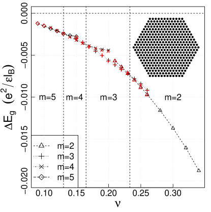
Figure 1: Variational ground state energies of CPWCs relative to that of the ordinary WC. Red points indicate the results of Ref. Yi and Fertig (1998). The phase boundaries between CPWC phases with different values of $m$ are determined by comparing the energies, and indicated by dashed vertical lines. Inset: configuration of the simulation cell.

Firstly, our calculation employs a much larger simulation cell which involves 397 electrons arranged as $11$ concentric hexagonal rings in a plane, as shown in the inset of Fig. (1). The larger simulation cell is needed to eliminate finite size effects as the coefficients decay slowly in the real space.

Secondly, we use a different wave function for the finite simulation cell, and eliminate the need for introducing “ghost” particles explicitly. As pointed out in Ref. Yi and Fertig (1998), for a finite lattice in equilibrium ($\bm{R}_{i}=\bm{R}_{i}^{0}$, and $\bm{k}_{i}=0$), the average positions of electrons do not coincide with their expected equilibrium positions due to asymmetry induced by the Bijl-Jastrow factor. As a result, it is necessary to introduce a cloud of “ghost particles” for each of electrons to counter balance the effect. In Ref. Yi and Fertig (1998), finite size ghost-particle clouds were introduced. In our simulation, we extend the size of the ghost particle clouds to infinity. The resulting wave function can be determined analytically:

$$\Psi\left(\left\{\bm{r}_{i}\right\}\right)\propto\mathcal{A}\frac{\prod_{i<j\leq N}(z_{i}+ik_{i}l_{B}^{2}-z_{j}-ik_{j}l_{B}^{2})^{m}}{\prod_{i\leq N}\prod_{j\neq i,\leq N}\left(z_{i}+ik_{j}l_{B}^{2}-Z_{j}^{0}\right)^{m}}\\ \times\prod_{i=1}^{N}\left[\psi(z_{i}-Z_{i}^{0}+ik_{i}l_{B}^{2})\right]^{m}\phi_{\bm{R}_{i}}(\bm{r}_{i}),$$ (51)

where $Z_{i}^{0}\equiv X_{i}^{0}+iY_{i}^{0}$ ($\bm{R}_{i}^{0}\equiv(X_{i}^{0},Y_{i}^{0})$), $N$ is the total number of electrons in the simulation cell, and Rhim et al. (2015),

$$\psi(z)\equiv\frac{\prod_{i\neq 0}\left(z-Z_{i}^{0}\right)}{\prod_{i\neq 0}\left(Z_{i}^{0}\right)}\propto\frac{1}{z}\theta_{1}\left(\left.\frac{z}{a}\right|\frac{1}{2}+i\frac{\sqrt{3}}{2}\right),$$ (52)

where $a$ is the lattice constant of the WC, the product is extended to an infinite triangular lattice with unit vectors $\bm{a}_{1}=(1,0)a$ and $\bm{a}_{2}=(1/2,\sqrt{3}/2)a$, and $\theta_{1}$ is the Jacobi theta function. Equation (51) is used in our numerical simulations.

An important issue of our simulation is to extrapolate the calculation results obtained in a finite simulation cell to the macroscopic limit. To this end, we find that $A_{0}^{\mathrm{finite}}$, coefficient defined in Eq. (15) calculated with a harmonic approximation of the wave function for the finite simulation cell (See Eq. (62) in Appendix B), fits the long-range tail of the calculated coefficient very well. Hence, we divide the coefficient into a long range part $A_{0}^{\mathrm{finite}}$ and a short range part that decays rapidly with the distance, and fit the short range part up to the fifth nearest neighbors. The extrapolation is then straightforward by upgrading $A_{0}^{\mathrm{finite}}$ to its infinite lattice counterpart, which can be determined analytically.

Similar extrapolation schemes are applied for the determinations of the coefficients Eq. (20–22). We can have harmonic approximation for these coefficients as well (see Eq. (64) in Appendix B). They are regarded as the long range parts of the coefficients. In this case, the remainders of the coefficients decays as $1/|\bm{R}_{i}^{0}-\bm{R}_{j}^{0}|^{5}$ in the long range. We fit the remainders of $\mathcal{D}^{\bm{x}\bm{x}}$ and $\mathcal{D}^{\bm{p}\bm{x}}$ with short range terms up to the fifth nearest neighbors, whereas for $\mathcal{D}^{\bm{p}\bm{p}}$, the higher precision of the calculated values allows us to fit it with a $1/|\bm{R}_{i}^{0}-\bm{R}_{j}^{0}|^{5}$ term plus the short range terms. We note that using the short-range terms to fit the remainders may yield an incorrect asymptotic behavior in the long wavelength limit. It makes our determination of the dynamic matrix less reliable in the regime.

Figure 1 shows the variational ground state energies determined from our simulations, and a comparison with the results presented in Ref. Yi and Fertig (1998). In our simulations, each of Markov chains contains a total $5.6\times 10^{12}$ proposal states with an acceptance rate $\sim 25\%$. They yield essentially identical results as the old simulations (within the error bars of the old simulations) albeit with much improved precision.

IV.2 Results

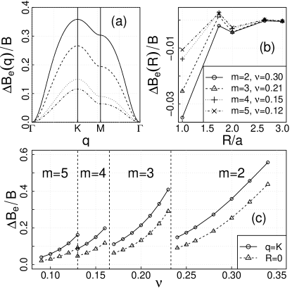
Figure 2: Emergent gauge field. (a) Distribution of the emergent gauge field in the Brillouin zone for four representative filling factors (see legends in (b)) with different values of $m$; (b) Decay of the dissipationless viscosity coefficient $\Delta\mathcal{B}_{e}(\bm{R}_{i}^{0})$ in the real space. $R$ denotes the distance between two particles, and $a$ is the lattice constant; (c) Filling factor $\nu$ dependence of the emergent gauge field at the $K$-point of the Brillouin zone (circle-solid line) and the mean-field value $\Delta B$ defined in (46) (triangle-dashed line ).

Figure 2 shows the emergent gauge field $\Delta B_{e}$. The distribution of the emergent field in the Brillouin zone is shown in Fig. 2(a). It peaks at the $K$-point and vanishes at the $\Gamma$-point. In the real space, the dissipationless viscosity coefficient decays rapidly with the distance, as shown in Fig. 2(b).

The strength of the emergent gauge field is characterized either by the value of $\Delta B_{e}(\bm{q})$ at the $K$-point or the mean-field value $\Delta B$ defined in Eq. (46). Both are shown in Fig. 2(c). The magnitude of the emergent field is ranged from a few percents to tens percents of the external magnetic field, and is an increasing function of the filling factor for a given value of $m$. The magnitude is smaller than that expected for a FQH liquid, which has a mean-field value $\Delta B^{FQH}/B=m\nu$. It indicates the mean-field approximation adopted for the theory of FQH liquids is not applicable for the CPWCs. On the other hand, the magnitude is actually gigantic in comparing with that generated by an intrinsic SOC. For instance, the intrinsic SOC in GaAs could also give rise to a similar emergent gauge field in an ordinary 2D WC. However, its magnitude is of order of $\sim 0.01\,\mathrm{T}$ only Ji and Shi (2017).

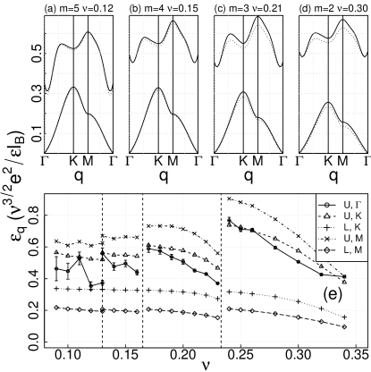
Figure 3: Phonon dispersions of type-I CPWCs. (a–d) Phonon dispersions for a few representative filling factors. Both results using the projected dynamic matrix (solid lines) and the unprojected one (dotted lines) are shown. (e) Filling factor $\nu$ dependence of phonon energies of the upper (U) and the lower (L) branch at high symmetry points of the Brillouin zone, including $K$ point, $M$ point, as well as $\Gamma$ point (evaluated at $\bm{q}=0.01\bm{K}$). $e^{2}/\epsilon l$ ($\approx 4.3\sqrt{B[\mathrm{T}]}\,\mathrm{meV}$ for GaAs) is the Coulomb energy scale. Error bars for the phonon energies near the $\Gamma$-point are shown.

The phonon dispersions of type-I CPWCs are obtained by solving the generalized eigenvalue equation Eq. (28). The results are summarized in Fig. 3. Among the two branches of phonons of a CPWC, the lower branch is not much different from that of an ordinary WC, both qualitatively and quantitatively Maki and Zotos (1983); Côté and MacDonald (1990, 1991), whereas the upper branch is an emergent mode with an energy scale $\sim 0.5\nu^{3/2}e^{2}/\epsilon l_{B}$, which is much smaller than the cyclotron energy. The upper branch has similar origin and energy scale as the magneto-roton mode arisen in FQH liquids Girvin et al. (1986). We thus interpret the mode as the magneto-roton mode of the CPWC.

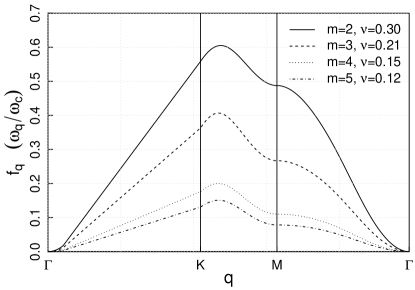
Figure 4: Oscillator strength of the emergent magneto-roton mode for a few representative filling factors, in unit of $\omega_{\bm{q}}/\omega_{c}$, where $\omega_{\bm{q}}$ is the frequency of the mode, and $\omega_{c}$ is the cyclotron frequency.

We also calculate the oscillator strength of the emergent magneto-roton mode. To do that, we determine the response of the system to an external time-dependent electric field $\bm{E}(t)=\bm{E}_{\omega}\exp(-i\omega t)$. Because the external electric field is only coupled to the electron degree of freedom (see Sec. III.2), it will introduce a scale potential $e\bm{E}(t)\cdot\bm{x}^{e}\equiv e\bm{E}(t)\cdot(\bm{x}-\hat{z}\times\bm{p}/eB)$ into the system. The extra term in the potential could be interpreted as a coupling to the dipole of a CP. As a result, the equation of motion has the form:

$$\left[\begin{array}[]{cc}eB_{e}(\bm{q})\hat{z}\times&I\\ -I&\frac{1}{eB}\hat{z}\times\end{array}\right]\left[\begin{array}[]{c}\dot{\bm{x}}(\bm{q})\\ \dot{\bm{p}}(\bm{q})\end{array}\right]=-\mathcal{D}(\bm{q})\left[\begin{array}[]{c}\bm{x}(\bm{q})\\ \bm{p}(\bm{q})\end{array}\right]\\ +\left[\begin{array}[]{c}-e\bm{E}(t)\\ \bm{E}(t)\times\hat{z}/B\end{array}\right].$$ (53)

By solving the equation, we can determine the displacement of electrons parallel to the electric field, and the oscillator strength $f_{\bm{q}i}$ is defined by the relation John David Jackson (1999) $x_{e}^{\parallel}(\bm{q})=-e/m_{b}\sum_{i}f_{\bm{q}i}/(\omega_{\bm{q}i}^{2}-\omega^{2}-i\omega 0^{+})E_{\omega}$, where $m_{b}$ is the electron band mass of the 2DEG. The oscillator strength for the emergent magneto-roton mode is shown in Fig. 4. We see that it vanishes at the limit $\bm{q}\rightarrow 0$, consistent with Kohn’s theorem.

The mode we predict here has an energy scale $\sim 0.5\nu^{3/2}e^{2}/\epsilon l_{B}$. For typical experimental parameters, the energy is much larger than that probed by existing microwave experiments Andrei et al. (1988); Engel et al. (1997); Li et al. (1997, 2000); Chen et al. (2003, 2004, 2006); Zhu et al. (2010); Williams et al. (1991), which are focused on the disorder pining modes. Our prediction thus calls for new microwave experiments to probe the new energy regime.

V Concluding remarks

In summary, we have derived the effective dynamics of CPs in a CPWC directly from the microscopic wave function. We find, most notably, the presence of a Berry curvature in the momentum space. The picture emerged from the dynamics is different from the conventional CF theory which assumes that CPs behave just like an ordinary Newtonian particle. On the other hand, we show that the dynamics is consistent with the dipole picture of CPs, and the presence of the Berry curvature is actually an inevitable consequence of the picture. The consistency is not a coincidence, since both are based on microscopic wave functions.

Although our theory is developed for the CPWC phase, the insight may be carried over to the liquid phase. In particular, the presence of the Berry curvature would provide a cure for deficiencies of the conventional CF theory Shi (2017). The solution is less radical and would be more natural compared to that prescribed by the Dirac theory Son (2015).

Our study reveals the discrepancy between the conventional interpretation of CPs and that emerged from a microscopic wave function. This is not surprising because the conventional picture was developed from a flux-attachment argument for free particles residing in a parabolic band Lopez and Fradkin (1991), while the microscopic wave functions are constructed for electrons constrained in a Landau level. For the latter, it would be highly desirable to have a CF theory which makes no direct reference to the magnetic field, since in a Landau level all the effects of the magnetic field has been accounted for by the Berry curvature. Indeed, in our dynamics, all the references to the magnetic field $eB$ could be interpreted as $1/\Omega_{z}$. Such a theory would also be a first step toward an understanding of the fractional Chern insulators Parameswaran et al. (2013).

Appendix A Dynamic matrix

To derive the formulas for the dynamic matrix coefficients (20–22), we make use identities:

$$\frac{\partial V_{ee}}{\partial x_{i\alpha}} =\frac{\partial V_{ee}}{\partial u_{j\beta}}\left[A^{-1}\right]_{j\beta,i\alpha},$$ (54)

$$\frac{\partial V_{ee}}{\partial p_{i\alpha}} =\frac{1}{\hbar}\left(\frac{\partial}{\partial k_{i\alpha}}-l_{B}^{2}\epsilon_{\alpha\beta}\frac{\partial}{\partial u_{i\beta}}\right)V_{ee},$$ (55)

$$\frac{\partial\left|\Psi\right|^{2}}{\partial u_{i\alpha}} =\frac{r_{i\alpha}-R_{i\alpha}}{l_{B}^{2}}\left|\Psi\right|^{2},$$ (56)

$$\frac{\partial\left|\Psi\right|^{2}}{\partial p_{i\alpha}} =\frac{1}{\hbar}\left(\frac{\partial}{\partial k_{i\alpha}}-l_{B}^{2}\epsilon_{\alpha\beta}\frac{\partial}{\partial u_{i\beta}}\right)\left|\Psi\right|^{2}=\frac{l_{B}^{2}}{\hbar}\epsilon_{\alpha\beta}\frac{\partial\left|\Psi\right|^{2}}{\partial r_{i\beta}}.$$ (57)

In deriving the last identity, we make use Eq. (10). We obtain:

$$\frac{\partial V_{ee}}{\partial x_{i\alpha}} =\frac{1}{l_{B}^{2}}\left\langle\left(\hat{V}_{ee}-\bar{V}_{ee}\right)\left(\hat{r}_{j\beta}-R_{j\beta}\right)\right\rangle\left[A^{-1}\right]_{j\beta,i\alpha},$$ (58)

$$\frac{\partial V_{ee}}{\partial p_{i\alpha}} =-\frac{l_{B}^{2}}{\hbar}\epsilon_{\alpha\beta}\left\langle\frac{\partial\hat{V}_{ee}}{\partial r_{i\beta}}\right\rangle\,.$$ (59)

Applying the second derivative, and making use the identities again, we obtain Eqs. (20–22).

Appendix B Harmonic approximations of the coefficients

A rudimentary approximation for evaluating the coefficients is the harmonic approximation. We define the harmonic approximation of the wave function as:

$$\left|\Psi_{0}\right|^{2}\propto\exp\left[2m\sum_{i<j}\ln\left|\bm{r}_{i}-\bm{r}_{j}\right|^{2}-\frac{1}{2l_{B}^{2}}\sum_{i}\left|\bm{r}_{i}-\bm{R}_{i}^{0}\right|^{2}\right]\\ \approx\exp\left[-\frac{1}{2}\sum_{ij,\alpha\beta}F_{\alpha\beta}(\bm{R}_{i}^{0}-\bm{R}_{j}^{0})\xi_{i\alpha}\xi_{j\beta}\right],$$ (60)

where

$$F_{\alpha\beta}(\bm{R}_{i}^{0})=\begin{cases}\frac{1}{l_{B}^{2}}\delta_{\alpha\beta}&\bm{R}_{i}^{0}=0\\ -2m\frac{2R_{i\alpha}^{0}R_{i\beta}^{0}-\left|\bm{R}_{i}^{0}\right|^{2}\delta_{\alpha\beta}}{\left|\bm{R}_{i}^{0}\right|^{4}}&\bm{R}_{i}^{0}\neq 0\end{cases}.$$ (61)

Under the approximation, the coefficient $A$ defined in Eq. (15) is related to $F$ by a matrix inversion:

$$A\approx A_{0}\equiv\frac{1}{l_{B}^{2}}F^{-1}.$$ (62)

The coefficient $F_{\alpha\beta}(\bm{R}_{i}^{0})$ satisfies an identity:

$$\sum_{\alpha}F_{\alpha\alpha}(\bm{R}_{i}^{0})=\frac{2}{l_{B}^{2}}\delta_{\bm{R}_{i}^{0},0}.$$ (63)

It leads to a vanishing emergent gauge field.

To evaluate the dynamic matrix, we first expand the electron-electron interaction operator $\hat{V}_{ee}$ to the second order of $\hat{\bm{\xi}}_{i}$. With the approximated wave function Eq. (60), the coefficients (20–22) become Gaussian integrals. We obtain the harmonic approximation of the dynamic matrix:

$$\mathcal{D}_{0}(\bm{q})=\left[\begin{array}[]{cc}D_{0}(\bm{q})&\frac{l_{B}^{2}}{\hbar}D_{0}(\bm{q})\hat{\epsilon}\\ -\frac{l_{B}^{2}}{\hbar}\hat{\epsilon}D_{0}(\bm{q})&-\frac{l_{B}^{4}}{\hbar^{2}}\hat{\epsilon}D_{0}(\bm{q})\hat{\epsilon}\end{array}\right],$$ (64)

where $D_{0}(\bm{q})$ is the $2\times 2$ classical dynamic matrix of the WC.

References

- Jainendra K. Jain (2007) Jainendra K. Jain, Composite fermions (Cambridge University Press, 2007).
- Jain and Anderson (2009) J. K. Jain and P. W. Anderson, “Beyond the Fermi Liquid Paradigm: Hidden Fermi Liquids,” Proceedings of the National Academy of Sciences 106, 9131 (2009).
- O. Heinonen (1997) O. Heinonen, Composite Fermions: A Unified View of the Quantum Hall Regime (World Scientific, 1997).
- Halperin et al. (1993) B. I. Halperin, P. A. Lee, and N. Read, “Theory of the half-filled Landau level,” Phys. Rev. B 47, 7312 (1993).
- Zhang (1992) S. C. Zhang, “The chern–simons–landau–ginzburg theory of the fractional quantum hall effect,” Int. J. Mod. Phys. B 06, 25 (1992).
- Moore and Read (1991) G. Moore and N. Read, “Nonabelions in the fractional quantum hall effect,” Nuclear Physics B 360, 362 (1991).
- Gabriele Giuliani and Giovanni Vignale (2005) Gabriele Giuliani and Giovanni Vignale, Quantum theory of the electron liquid (Cambridge University Press, 2005).
- Yi and Fertig (1998) H. Yi and H. A. Fertig, “Laughlin-Jastrow-correlated Wigner crystal in a strong magnetic field,” Phys. Rev. B 58, 4019 (1998).
- Narevich et al. (2001) R. Narevich, G. Murthy, and H. A. Fertig, “Hamiltonian theory of the composite-fermion Wigner crystal,” Phys. Rev. B 64, 245326 (2001).
- Archer et al. (2013) A. C. Archer, K. Park, and J. K. Jain, “Competing Crystal Phases in the Lowest Landau Level,” Phys. Rev. Lett. 111, 146804 (2013).
- Yang et al. (2001) K. Yang, F. D. M. Haldane, and E. H. Rezayi, “Wigner crystals in the lowest Landau level at low-filling factors,” Phys. Rev. B 64, 081301 (2001).
- Lee et al. (2002) S.-Y. Lee, V. W. Scarola, and J. Jain, “Structures for interacting composite fermions: Stripes, bubbles, and fractional quantum Hall effect,” Phys. Rev. B 66, 085336 (2002).
- Goerbig et al. (2004) M. O. Goerbig, P. Lederer, and C. Morais Smith, “Possible Reentrance of the Fractional Quantum Hall Effect in the Lowest Landau Level,” Phys. Rev. Lett. 93, 216802 (2004).
- Chang et al. (2005) C.-C. Chang, G. S. Jeon, and J. K. Jain, “Microscopic Verification of Topological Electron-Vortex Binding in the Lowest Landau-Level Crystal State,” Phys. Rev. Lett. 94, 016809 (2005).
- Chang et al. (2006) C.-C. Chang, C. Töke, G. S. Jeon, and J. K. Jain, “Competition between composite-fermion-crystal and liquid orders at =1/5,” Phys. Rev. B 73, 155323 (2006).
- Andrei et al. (1988) E. Y. Andrei, G. Deville, D. C. Glattli, F. I. B. Williams, E. Paris, and B. Etienne, “Observation of a Magnetically Induced Wigner Solid,” Phys. Rev. Lett. 60, 2765 (1988).
- Engel et al. (1997) L. W. Engel, C. C. Li, D. Shahar, D. C. Tsui, and M. Shayegan, “Microwave resonances in low-filling insulating phases of two-dimensional electron and hole systems,” Physica E: Low-dimensional Systems and Nanostructures 1, 111 (1997).
- Li et al. (1997) C.-C. Li, L. W. Engel, D. Shahar, D. C. Tsui, and M. Shayegan, “Microwave Conductivity Resonance of Two-Dimensional Hole System,” Phys. Rev. Lett. 79, 1353 (1997).
- Li et al. (2000) C.-C. Li, J. Yoon, L. W. Engel, D. Shahar, D. C. Tsui, and M. Shayegan, “Microwave resonance and weak pinning in two-dimensional hole systems at high magnetic fields,” Phys. Rev. B 61, 10905 (2000).
- Chen et al. (2003) Y. Chen, R. M. Lewis, L. W. Engel, D. C. Tsui, P. D. Ye, L. N. Pfeiffer, and K. W. West, “Microwave Resonance of the 2d Wigner Crystal around Integer Landau Fillings,” Phys. Rev. Lett. 91, 016801 (2003).
- Chen et al. (2004) Y. P. Chen, R. M. Lewis, L. W. Engel, D. C. Tsui, P. D. Ye, Z. H. Wang, L. N. Pfeiffer, and K. W. West, “Evidence for Two Different Solid Phases of Two-Dimensional Electrons in High Magnetic Fields,” Phys. Rev. Lett. 93, 206805 (2004).
- Chen et al. (2006) Y. P. Chen, G. Sambandamurthy, Z. H. Wang, R. M. Lewis, L. W. Engel, D. C. Tsui, P. D. Ye, L. N. Pfeiffer, and K. W. West, “Melting of a 2d quantum electron solid in high magnetic field,” Nat Phys 2, 452 (2006).
- Zhu et al. (2010) H. Zhu, Y. P. Chen, P. Jiang, L. W. Engel, D. C. Tsui, L. N. Pfeiffer, and K. W. West, “Observation of a Pinning Mode in a Wigner Solid with $\ensuremath{\nu}=1/3$ Fractional Quantum Hall Excitations,” Phys. Rev. Lett. 105, 126803 (2010).
- Williams et al. (1991) F. I. B. Williams, P. A. Wright, R. G. Clark, E. Y. Andrei, G. Deville, D. C. Glattli, O. Probst, B. Etienne, C. Dorin, C. T. Foxon, and J. J. Harris, “Conduction threshold and pinning frequency of magnetically induced Wigner solid,” Phys. Rev. Lett. 66, 3285 (1991).
- Zhang et al. (2015) C. Zhang, R.-R. Du, M. J. Manfra, L. N. Pfeiffer, and K. W. West, “Transport of a sliding Wigner crystal in the four flux composite fermion regime,” Phys. Rev. B 92, 075434 (2015).
- Liu et al. (2014) Y. Liu, D. Kamburov, S. Hasdemir, M. Shayegan, L. N. Pfeiffer, K. W. West, and K. W. Baldwin, “Fractional Quantum Hall Effect and Wigner Crystal of Interacting Composite Fermions,” Phys. Rev. Lett. 113, 246803 (2014).
- Pan et al. (2002) W. Pan, H. L. Stormer, D. C. Tsui, L. N. Pfeiffer, K. W. Baldwin, and K. W. West, “Transition from an Electron Solid to the Sequence of Fractional Quantum Hall States at Very Low Landau Level Filling Factor,” Phys. Rev. Lett. 88, 176802 (2002).
- Li et al. (1991) Y. P. Li, T. Sajoto, L. W. Engel, D. C. Tsui, and M. Shayegan, “Low-frequency noise in the reentrant insulating phase around the 1/5 fractional quantum Hall liquid,” Phys. Rev. Lett. 67, 1630 (1991).
- Jiang et al. (1991) H. W. Jiang, H. L. Stormer, D. C. Tsui, L. N. Pfeiffer, and K. W. West, “Magnetotransport studies of the insulating phase around \ensuremath{\nu}=1/5 Landau-level filling,” Phys. Rev. B 44, 8107 (1991).
- Jiang et al. (1990) H. W. Jiang, R. L. Willett, H. L. Stormer, D. C. Tsui, L. N. Pfeiffer, and K. W. West, “Quantum liquid versus electron solid around =1/5 Landau-level filling,” Phys. Rev. Lett. 65, 633 (1990).
- Goldman et al. (1990) V. J. Goldman, M. Santos, M. Shayegan, and J. E. Cunningham, “Evidence for two-dimentional quantum Wigner crystal,” Phys. Rev. Lett. 65, 2189 (1990).
- Maki and Zotos (1983) K. Maki and X. Zotos, “Static and dynamic properties of a two-dimensional Wigner crystal in a strong magnetic field,” Phys. Rev. B 28, 4349 (1983).
- Côté and MacDonald (1990) R. Côté and A. H. MacDonald, “Phonons as collective modes: The case of a two-dimensional Wigner crystal in a strong magnetic field,” Phys. Rev. Lett. 65, 2662 (1990).
- Côté and MacDonald (1991) R. Côté and A. H. MacDonald, “Collective modes of the two-dimensional Wigner crystal in a strong magnetic field,” Phys. Rev. B 44, 8759 (1991).
- Simon (1998) S. H. Simon, “The chern-simons fermi liquid description of fractional quantum hall states,” in Composite Fermions (World Scientific, 1998) pp. 91–194.
- Girvin et al. (1986) S. M. Girvin, A. H. MacDonald, and P. M. Platzman, “Magneto-roton theory of collective excitations in the fractional quantum Hall effect,” Phys. Rev. B 33, 2481 (1986).
- Rhim et al. (2015) J.-W. Rhim, J. K. Jain, and K. Park, “Analytical theory of strongly correlated Wigner crystals in the lowest Landau level,” Phys. Rev. B 92, 121103 (2015).
- Archer and Jain (2011) A. C. Archer and J. K. Jain, “Static and dynamic properties of type-II composite fermion Wigner crystals,” Phys. Rev. B 84, 115139 (2011).
- Ettouhami et al. (2006) A. M. Ettouhami, F. D. Klironomos, and A. T. Dorsey, “Static and dynamic properties of crystalline phases of two-dimensional electrons in a strong magnetic field,” Phys. Rev. B 73, 165324 (2006).
- Lopez and Fradkin (1991) A. Lopez and E. Fradkin, “Fractional quantum Hall effect and Chern-Simons gauge theories,” Phys. Rev. B 44, 5246 (1991).
- Sundaram and Niu (1999) G. Sundaram and Q. Niu, “Wave-packet dynamics in slowly perturbed crystals: Gradient corrections and Berry-phase effects,” Phys. Rev. B 59, 14915 (1999).
- Xiao et al. (2010) D. Xiao, M.-C. Chang, and Q. Niu, “Berry phase effects on electronic properties,” Rev. Mod. Phys. 82, 1959 (2010).
- Qin et al. (2012) T. Qin, J. Zhou, and J. Shi, “Berry curvature and the phonon Hall effect,” Phys. Rev. B 86, 104305 (2012).
- Hughes et al. (2011) T. L. Hughes, R. G. Leigh, and E. Fradkin, “Torsional Response and Dissipationless Viscosity in Topological Insulators,” Phys. Rev. Lett. 107, 075502 (2011).
- Son (2015) D. T. Son, “Is the Composite Fermion a Dirac Particle?” Phys. Rev. X 5, 031027 (2015).
- Son (2016) D. T. Son, “The Dirac composite fermion of the fractional quantum Hall effect,” Prog Theor Exp Phys 2016, 12C103 (2016).
- Read (1994) N. Read, “Theory of the half-filled Landau level,” Semicond. Sci. Technol. 9, 1859 (1994).
- Rezayi and Read (1994) E. Rezayi and N. Read, “Fermi-liquid-like state in a half-filled Landau level,” Phys. Rev. Lett. 72, 900 (1994).
- P. Kramer and M. Saraceno (1981) P. Kramer and M. Saraceno, Geometry of the Time-Dependent Variational Principle in Quantum Mechanics (Springer, 1981).
- Note (1) We have assumed that the direction of is along direction, where is the charge of a carrier, and is the normal direction of the 2DEG plane. For the opposite case, one should define instead.
- Kalmeyer and Zhang (1992) V. Kalmeyer and S.-C. Zhang, “Metallic phase of the quantum Hall system at even-denominator filling fractions,” Phys. Rev. B 46, 9889 (1992).
- Xiao et al. (2005) D. Xiao, J. Shi, and Q. Niu, “Berry Phase Correction to Electron Density of States in Solids,” Phys. Rev. Lett. 95, 137204 (2005).
- Glauber (1963) R. J. Glauber, “Coherent and Incoherent States of the Radiation Field,” Phys. Rev. 131, 2766 (1963).
- Jungwirth et al. (2002) T. Jungwirth, Q. Niu, and A. H. MacDonald, “Anomalous Hall Effect in Ferromagnetic Semiconductors,” Phys. Rev. Lett. 88, 207208 (2002).
- Haldane (1988) F. D. M. Haldane, “Model for a Quantum Hall Effect without Landau Levels: Condensed-Matter Realization of the "Parity Anomaly",” Phys. Rev. Lett. 61, 2015 (1988).
- Zhang and Shi (2016) Y. Zhang and J. Shi, “Mapping a fractional quantum Hall state to a fractional Chern insulator,” Phys. Rev. B 93, 165129 (2016).
- Shi (2017) J. Shi, “Chern-Simons Theory and Dynamics of Composite Fermions,” arXiv:1704.07712 [cond-mat] (2017).
- Potter et al. (2016) A. C. Potter, M. Serbyn, and A. Vishwanath, “Thermoelectric Transport Signatures of Dirac Composite Fermions in the Half-Filled Landau Level,” Phys. Rev. X 6, 031026 (2016).
- Ji and Shi (2017) W.-C. Ji and J.-R. Shi, “Topological Phonon Modes in a Two-Dimensional Wigner Crystal,” Chinese Phys. Lett. 34, 036301 (2017).
- John David Jackson (1999) John David Jackson, Classical electrodynamics (Wiley, 1999).
- Parameswaran et al. (2013) S. A. Parameswaran, R. Roy, and S. L. Sondhi, “Fractional quantum Hall physics in topological flat bands,” Comptes Rendus Physique Topological insulators / Isolants topologiques, 14, 816 (2013).