Differential topology of semimetals

Varghese Mathai Address: Department of Pure Mathematics, University of Adelaide, Adelaide 5005, Australia Email address: mathai.varghese@adelaide.edu.au and Guo Chuan Thiang Address: Department of Pure Mathematics, University of Adelaide, Adelaide 5005, Australia Email address: guochuan.thiang@adelaide.edu.au
Abstract.

The subtle interplay between local and global charges for topological semimetals exactly parallels that for singular vector fields. Part of this story is the relationship between cohomological semimetal invariants, Euler structures, and ambiguities in the connections between Weyl points. Dually, a topological semimetal can be represented by Euler chains from which its surface Fermi arc connectivity can be deduced. These dual pictures, and the link to topological invariants of insulators, are organised using geometric exact sequences. We go beyond Dirac-type Hamiltonians and introduce new classes of semimetals whose local charges are subtle Atiyah–Dupont–Thomas invariants globally constrained by the Kervaire semicharacteristic, leading to the prediction of torsion Fermi arcs.

Key words and phrases:
Topological semimetals, Topological insulators, Fermi arcs, Euler structures, Euler characteristic, Poincaré–Hopf theorem, Kervaire structures, Kervaire semicharacteristic, Atiyah–Dupont theorem, Mayer–Vietoris sequence, Gysin sequence
2010 Mathematics Subject Classification
81H20, 82D35

1. Introduction

As theoretically predicted in [70] and experimentally discovered in [73, 74, 37, 76], two-band solid state systems in 3D can host topologically protected “Weyl semimetallic phases” in which the quasiparticle excitations at the band crossings (“Weyl points”) share some features with Weyl fermions from relativistic quantum mechanics. The experimental signature, namely “Fermi arcs” of surface states which connect the projected Weyl points in the surface Brillouin zone, is just as remarkable. Based on this initial success, much effort has been put into the general study of topological semimetallic phases in the hope of predicting and eventually realising new exotic fermionic quasiparticles in condensed matter systems.

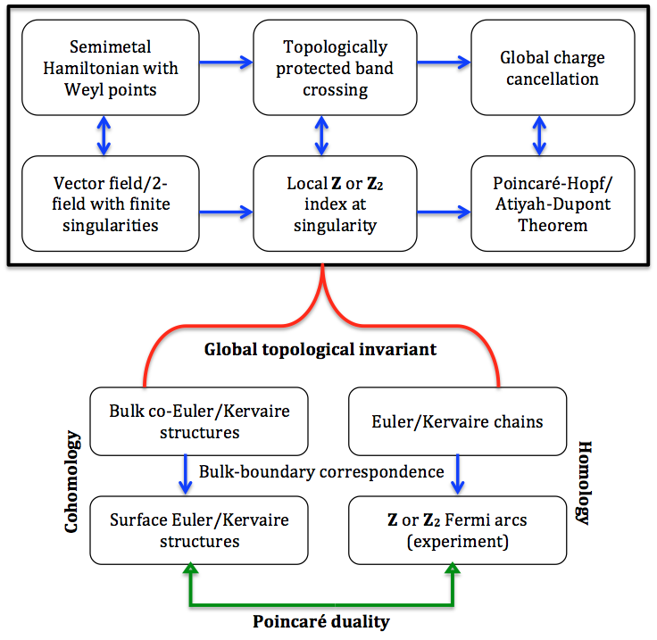
Most proposals have focused on local aspects in the sense of finding new types of topological obstructions to locally opening up gaps in semimetal band crossings. Staying in the two-band case, there are generalisations of the basic Weyl semimetal phase to “Type-II” ones [75, 57], as well as “quadratic” ones [25]. One can consider model Hamiltonians with more than two bands and in a different number of spatial dimensions [77]. Following the example set by topological insulator theory, one may also introduce antiunitary symmetry constraints such as time-reversal and charge-conjugation [78]. To circumvent certain difficulties in achieving non-trivial obstructions, point symmetries were also introduced into the game, and a host of possibilities arise [10]. Our results in this paper have a different focus, concentrating on (1) isolating in a conceptually simple but rigorous way the general mathematical mechanism allowing for local semimetallic charges, (2) providing the full global topological characterisation of semimetal band structures, Fermi arcs, and the relation to topological insulator invariants, and (3) introducing a new family of semimetals whose topological invariants have a very different character to those commonly used in the literature. Figure 1 summarises the physical and mathematical concepts which we introduce in this paper.
Refer to caption
Figure 1. Semimetals have Bloch Hamiltonians with band crossings at certain isolated Weyl points in the Brillouin torus TT, corresponding to vector fields over TT with finite isolated singularities at the Weyl points. These band crossings may be topologically protected, with their {\mathbb{Z}} topological charges corresponding to the local indices of the vector field at the singularities. The charge-cancellation condition corresponds to the Poincaré–Hopf theorem. The global semimetal band structure can be studied in two complementary ways (Definition 3.6) which are dual to each other and related by Poincaré duality. Semimetals have characteristic classes in cohomology, identifiable as co-Euler structures, while in homology they are represented by the dual Euler chains. Under a bulk-boundary correspondence, these invariants are mapped to surface invariants, which in homology is just the projection of the Euler chain onto the Fermi arcs seen in experiments. These ideas can be generalised to semimetal Hamiltonians specified by tangent 2-fields, which now have 2{\mathbb{Z}}_{2}-charges. Euler structures and chains are replaced by Kervaire ones, and the Poincaré–Hopf theorem replaced by a theorem of Atiyah–Dupont.

With regards to (1), we see, with much hindsight, that the local topological charges protecting basic types of semimetal crossings are completely inherited from the singular vector field which specifies the Hamiltonian [72, 41]. The Poincaré–Hopf theorem [43] then shows how the Brillouin zone topology forces a global charge cancellation condition, and the prediction of Fermi arcs becomes a corollary of the bulk-boundary correspondence. This brings us to point (2). While the 3D Weyl semimetal may be intuitively understood using a Stokes’ Theorem argument to predict “jumps” in 2D Chern numbers (or “weak invariants”) across the Weyl points, there are several subtleties involved, not the least of which is the fact that the local charges (equal to the jumps) fail to completely characterise the semimetal, and cannot predict, a priori, the Fermi arc topology [41]. It is here that the finer topology of the Brillouin torus comes into play: the fact that 𝕋d{\mathbb{T}}^{d} has non-trivial cycles means that “the (Fermi) arc joining two Weyl points” is an ambiguous notion, even up to deformations of the arc (contrast with the simply-connected spheres). The resolution of this ambiguity requires additional global data which captures the full topology of semimetal band structures, and is closely related to the concept of Euler structures introduced by Turaev to resolve ambiguities in torsions of Reidemeister type [65]; both hinge on the fact that the first homology of the underlying manifold may be non-zero. By considering a homological version of Euler structures [12, 26], we find that the language of Euler chains very concisely represents all the topological features of a semimetal. The Euler chain representation directly predicts the topology of the Fermi arcs, and the latter are the experimental signature of a topological semimetal. Furthermore, the notion of topological equivalence between semimetals becomes clear in this language, as a kind of homotopy between their defining vector fields. A semimetal Hamiltonian determines a Fermi arc, e.g. through a transfer matrix formalism [22, 4, 17], and this determination descends to the level of topological invariants in the sense that equivalent Hamiltonians give rise to equivalent Fermi arcs.

Having isolated the basic mathematical principles underlying the geometry and topology of semimetals, we move on to (3): the generalisation of our theory for 2-frames or tangent 2-fields along the lines of the Atiyah–Dupont theorem [2] which is the analogue of the Poincaré--Hopf theorem11 1 The latter accounts for the Nielsen–Ninomiya no-go theorem [48] excluding chiral fermions in lattice gauge theory. in this context, where the Kervaire semicharacteristic plays the role of the Euler characteristic. It is a topological invariant of a very different nature to those that had been previously utilised in the literature on topological phases (e.g. Chern classes and related characteristic classes, KK-theory, winding numbers/degrees). This leads us to define some new mathematical notions — Kervaire structures and Kervaire chains — which are two mutually dual objects characterising a new class of 2{\mathbb{Z}}_{2}-topological semimetals introduced for the first time in this paper, predicting in principle that torsion Fermi arcs can be experimentally found.

1.1. Outline

In Section 2, we give a quick overview of the use of cohomological characteristic classes to study topological insulating phases, and then connect it to semimetal phases via the Mayer–Vietoris technique of “patching together” the non-singular portion (avoiding the Weyl points) and topologically trivial portions (small neighbourhoods of the Weyl points). The basic “semimetal Mayer–Vietoris sequence” is given a geometric interpretation as an extension problem, parallel to the physical problem of deforming a semimetal band structure into a globally insulating one, in Section 2.5. In Section 3, we introduce the concept of Euler structures and the Euler chain representation of a semimetal. We illustrate with diagrams the basic intuitive ideas, and apply the Euler chain concept to Fermi arc topology and their rewirings. In Section 4, we study Dirac-type Hamiltonians parametrised by singular vector fields, emphasising the merits of an abstract coordinate-free analysis with regards to symmetry considerations. In particular, we justify the generality of Dirac-type Hamiltonians through natural symmetry constraints, in order to avoid introducing “spurious topology” through ad-hoc parametrisations of toy model Hamiltonians. In Section 4.6.1, a geometric connection to gerbes is made in the 4D case (we refer the reader to Appendix A for a primer on gerbes and the construction of the basic gerbe on SU(2)\text{SU}(2)), and in Section 4.5, the connection to quaternionic valence bundles in 5D is made, and the geometric interpretation as an extension problem is in Section 2.5. In Section 5, we introduce a new class of semimetals modelled on Hamiltonians which are bilinear in gamma matrices. The topology of such semimetals is characterised by the notion of Kervaire structures and chains, and we predict an interesting phenomenon of 2{\mathbb{Z}}_{2} surface Fermi arcs. Finally we suggest some directions for future work in Section 6.

Conventions. In this paper, TT will always be a compact connected smooth dd-dimensional manifold without boundary, playing the role of a general parameter manifold for a family of Hamiltonians. In specific instances, it may have an orientation, metric, spinc structure etc., and may be the Brillouin zone for a family of Bloch Hamiltonians, as additionally specified. All (co)-homology groups have integer coefficients unless otherwise indicated. The real Clifford algebra Clr,sCl_{r,s} has rr generators squaring to 1-1 and ss generators squaring to +1+1, corresponding to an orthonormal basis e1,.,er+se_{1},.\ldots,e_{r+s} in r+s{\mathbb{R}}^{r+s} for the bilinear form (,,,++)(-,\ldots,-,+\ldots+); ClnCl_{n} refers to Cl0,nCl_{0,n}, and the complex Clifford algebra ln{\mathbb{C}}l_{n} has nn anticommuting generators squaring to +1+1.

2. Physical background: Topological phases, cohomology

2.1. Topological band insulators and cohomology groups

2D Chern insulators are classified by a first Chern number, equal to the integrated Berry curvature 2-form of the valence bands over the Brillouin zone T=𝕋2T={\mathbb{T}}^{2}. When the Fermi energy EFE_{F} lies in a spectral gap, the Fermi projection onto the valence bundle F\mathcal{E}_{F} may be defined. Over 𝕋2{\mathbb{T}}^{2} the F\mathcal{E}_{F} are classified by their rank and first Chern class, with the latter generally considered to be the interesting invariant. Since the first Chern class of F\mathcal{E}_{F} is that of the determinant line bundle, the classification problem of 2D Chern insulators is formally equivalent to that of U(1) line bundles over the Brillouin zone for which the integral cohomology group H2(𝕋2,)H^{2}({\mathbb{T}}^{2},{\mathbb{Z}})\cong{\mathbb{Z}} provides a complete answer. In terms of differential forms, H2(𝕋2,)0H^{2}({\mathbb{T}}^{2},{\mathbb{Z}})\neq 0 measures the failure of the (Berry) curvature 2-form \mathcal{F} of F\mathcal{E}_{F} to be globally exact (the Berry connection 1-form 𝒜\mathcal{A} only exists locally). The integral of \mathcal{F} over 𝕋2{\mathbb{T}}^{2} yields an integer-valued first Chern number, which may be interpreted as a topological obstruction to globally defining a basis of valence Bloch eigenstates for F\mathcal{E}_{F}.

A typical way to construct a valence line bundle with first Chern class nn\in{\mathbb{Z}} is to consider 2×22\times 2 traceless22 2 We normalize the Fermi level to 00. Bloch Hamiltonians H(k)=𝒉(k)𝝈,k𝕋2H(k)=\bm{{h}}(k)\cdot\bm{{\sigma}},\,k\in{\mathbb{T}}^{2}, parametrised by a nowhere-vanishing smooth vector field 𝒉\bm{{h}} on 𝕋2{\mathbb{T}}^{2}. Here 𝝈=(σ1,σ2,σ3)\bm{{\sigma}}=(\sigma_{1},\sigma_{2},\sigma_{3}) are the Pauli matrices. The spectrum is ±|𝒉(k)|0\pm|\bm{{h}}(k)|\neq 0, and the spectrally-flattened Hamiltonian H^\widehat{H} is parametrised by the unit vector map 𝒉^:𝕋2S23\hat{\bm{{h}}}:{\mathbb{T}}^{2}\rightarrow S^{2}\subset{\mathbb{R}}^{3}. Note that HH and H^\widehat{H} determine the same valence line subbundle F\mathcal{E}_{F} of the Bloch bundle 𝕋2×2{\mathbb{T}}^{2}\times{\mathbb{C}}^{2}. The map 𝒉^\hat{\bm{{h}}} has an integer degree given by the formula 𝒉^([𝕋2])=deg(𝒉^)[S2]\hat{\bm{{h}}}_{*}([{\mathbb{T}}^{2}])=\text{deg}(\hat{\bm{{h}}})[S^{2}], where [𝕋2],[S2][{\mathbb{T}}^{2}],[S^{2}] denote the fundamental classes. The degree is a homotopy invariant, and all degrees do occur. By identifying S2S^{2} with 1{\mathbb{C}}{\mathbb{P}}^{1} (the Bloch sphere construction), we see that F\mathcal{E}_{F} is given by the pullback of the tautological (Hopf) line bundle over 1{\mathbb{C}}{\mathbb{P}}^{1} under 𝒉^\hat{\bm{{h}}}. Due to the low-dimensionality of 𝕋2{\mathbb{T}}^{2}, all maps into =K(,2){\mathbb{C}}{\mathbb{P}}^{\infty}=K({\mathbb{Z}},2) are approximated by maps into 1{\mathbb{C}}{\mathbb{P}}^{1}, and so the first Chern class of F\mathcal{E}_{F} is precisely the degree of 𝒉^\hat{\bm{{h}}}.

In higher dimensions, and also in the presence of additional symmetries (e.g. time-reversal or point group symmetries) constraining the form of the Hamiltonians, topological band insulators are classified by more complicated invariants. In the mathematical physics literature, these have included higher degree cohomology invariants playing the role of characteristic classes for the valence bundles, e.g. higher Chern/instanton numbers, symplectic bundle invariants [5, 6, 23], Fu–Kane–Mele/FKMM-type invariants [15], or generalised cohomology invariants (KK-theory) [19, 62]. We are primarily interested in 3,43,4 or 55 spatial dimensions, and in those dimensions, the relevant “Berry curvature form” \mathcal{F} can be a higher-degree form [14, 21, 34], and so a higher degree cohomology group Hn(X,)H^{n}(X,{\mathbb{Z}}) comes into play. Cohomology groups with other coefficients also arise quite generally in obstruction theory, which can be used to study semimetal-insulator transitions. All these (generalised) cohomological invariants are also homotopy invariants, and are closely related to degree theory (as we saw from the 2D Chern insulator described above).

2.2. Topological semimetals

Although the prototypical topological semimetal is the Weyl semimetal in d=3d=3, the general theory presented in this paper works in higher dimensions. This is not merely of theoretical interest. In the case of topological insulators, there are concrete proposals and experiments in which topological phases of physical systems in three or fewer dimensions formally realise those in d>3d>3. Some examples are quasicrystalline systems [31], time-periodic (Floquet) insulators [35, 14] and their photonic counterparts [53], and general “virtual” topological insulators [51]. It is in this spirit that we embark on the mathematical study of semimetallic phases for general dd.

2.2.1. Local aspects of semimetal topology

In a semimetal, the Fermi level does not lie in a spectral gap, but instead passes through band crossings at some Weyl submanifold WW of the momentum space manifold TT. Such crossings may arise as “accidental degeneracies” [69, 24] and, for “Dirac-type Hamiltonians” in dd-dimensions occur generically at points. A quick way to see this is to consider Dirac-type Bloch Hamiltonians of the form

(2.1) H(k)=𝒉(k)𝜸,kT;H(k)=\bm{{h}}(k)\cdot\bm{{\gamma}},\qquad k\in T;

Here each k𝒉(k)k\mapsto\bm{{h}}(k) is a smooth assignment of dd-component vectors, and 𝜸=(γ1,,γd)\bm{{\gamma}}=(\gamma_{1},\ldots,\gamma_{d}) is the vector of traceless Hermitian γ\gamma-matrices representing irreducibly and self-adjointly the dd-generators of a Clifford algebra (for d=3d=3, these are the usual 2×22\times 2 Pauli matrices). By the Clifford algebra relations γiγj+γjγi=2δij\gamma_{i}\gamma_{j}+\gamma_{j}\gamma_{i}=2\delta_{ij}, the square of H(k)H(k) is the scalar |𝒉(k)|2|\bm{{h}}(k)|^{2}, so the eigenvalues of H(k)H(k) are ±|𝒉(k)|\pm|\bm{{h}}(k)|, each with degeneracy equal to half the dimension of the γ\gamma-matrices. This means that a band crossing at kTk\in T requires dd conditions 𝒉(k)=𝟎\bm{{h}}(k)=\bm{{0}}, and we see that the locus WW of band crossings generically has codimension dd. When TT is a dd-manifold, WW is generically a collection of isolated “Weyl points”, the (rather misleading) terminology arising from the d=3d=3 case in which the low-energy excitations around a band crossing are essentially described by the Weyl equation [70, 67]. Furthermore, each Weyl point wWw\in W serves as a generalised monopole, and may be assigned a local topological charge via the unit-vector map restricted to a small enclosing d1d-1-sphere SwS_{w},

(2.2) 𝒉^w=𝒉(k)|𝒉(k)|:SwSd1d,d=3,4,5,\hat{\bm{{h}}}_{w}=\frac{\bm{{h}}(k)}{|\bm{{h}}(k)|}:S_{w}\longrightarrow S^{d-1}\subset{\mathbb{R}}^{d},\qquad d=3,4,5,

and defining the local charge at ww to be the degree of 𝒉^w\hat{\bm{{h}}}_{w}, equal to the local index Indw(𝒉)\text{Ind}_{w}(\bm{{h}}) of 𝒉\bm{{h}} at ww. The local charge information of all the crossings for the Hamiltonian 𝒉𝜸\bm{{h}}\cdot\bm{{\gamma}} is concisely summarised by the 0-chain 𝒲𝒉wWIndw(𝒉)wC0(T,)\mathcal{W}_{\bm{{h}}}\coloneqq\sum_{w\in W}\text{Ind}_{w}(\bm{{h}})w\in C_{0}(T,{\mathbb{Z}}), where Ci(,)C_{i}(\cdot,{\mathbb{Z}}) denotes the set of singular ii-chains.

The unit vector map 𝒉^\hat{\bm{{h}}} on TWT\setminus W, and its restrictions (2.2) to SwS_{w}, can be used to pullback the Hopf line bundle with connection when d=3d=3, the basic gerbe with connection when d=4d=4 and the quaternionic Hopf line bundle with connection when d=5d=5 (see Appendix A for their definitions). As explained in Section 2.5, these geometrical structures arise naturally when analysing Dirac-type Hamiltonians, their band crossings, and the topology of their valence bundles.

2.2.2. Global aspects of semimetal topology

Interesting phenomena arise when we study the band crossings globally. For instance, if 𝒉\bm{{h}} can be identified as a tangent vector field over TT, as is often the case in physical models, then the classical Poincaré–Hopf theorem guarantees that wWIndw(𝒉)=χ(T)=0\sum_{w\in W}\text{Ind}_{w}(\bm{{h}})=\chi(T)=0 where χ(T)\chi(T) is the Euler characteristic of TT, which is zero for T=𝕋dT={\mathbb{T}}^{d} or dd odd. This global “charge-cancellation” condition is well-known in lattice gauge theory (where T=𝕋dT={\mathbb{T}}^{d}) as the Nielsen–Ninomiya theorem [48] and discussed in the semimetal context in [72, 41]. Together with the bulk-boundary correspondence, it predicts the appearance of surface Fermi arcs connecting the projected Weyl points on a surface Brillouin zone. These arcs are an experimental signature of topological non-triviality in a semimetal band structure, and have been discovered recently [73, 37].

More generally, 𝒉\bm{{h}} could be a section of some oriented rank-dd vector bundle \mathcal{E} over a compact oriented dd-manifold TT. The local topological charges at the zeros of 𝒉\bm{{h}} are defined as before, as is the Euler characteristic of \mathcal{E} (evaluating the Euler class on the fundamental class). When the Euler characteristic χ\chi vanishes (and also when χ0\chi\neq 0 following [12]), a notion of Euler structures [65] can be defined. The set of Euler structures of TT form a torsor over H1(T,)H_{1}(T,{\mathbb{Z}}), and it provides an elegant way to understand some global aspects of Fermi arc topology, including certain ambiguities first studied in [41], the “rewiring” of Fermi arcs [18, 36], and Weyl point creation/annihilation (Section 3.1). This is already interesting when T=𝕋dT={\mathbb{T}}^{d}, for which there are non-trivial Euler structures: the various different ways of connecting two Weyl points by an arc are permuted amongst each other under H1(T,)H_{1}(T,{\mathbb{Z}}). We remark that Euler structures had previously been been used to clarify certain ambiguities in the Reidemeister torsion and Seiberg–Witten invariants of 3-manifolds. Their appearance in the semimetal context indicates a similar subtlety and richness in the structure of semimetals.

We take the following as a working definition:

Definition 2.1.

Let TT be a compact, oriented dd-dimensional Riemannian spinc manifold with d3d\geq 3. An abstract Dirac-type Hamiltonian is a smooth vector field 𝒉\bm{{h}} over TT, which is insulating if 𝒉\bm{{h}} is non-singular (nowhere zero), and semimetallic if 𝒉\bm{{h}} has a finite set WW of singularities.

This definition is motivated by the construction of concrete Bloch Hamiltonians from such vector fields, generalising (2.1), given in Section 4.

2.3. Mayer–Vietoris principle: connecting topological insulators and semimetals

In [41], we carried out an analysis of the global structure of semimetal band structures and Fermi arcs. The Mayer–Vietoris principle provided the key to understanding the connection between topological semimetals and insulators (Fig. 2). In particular, we showed that the local charge information at Weyl points needs to be supplemented with some global data to fully characterise semimetal band structure and Fermi arcs. We summarise the key constructions in [41], then provide several different ways to understand them.
Refer to caption
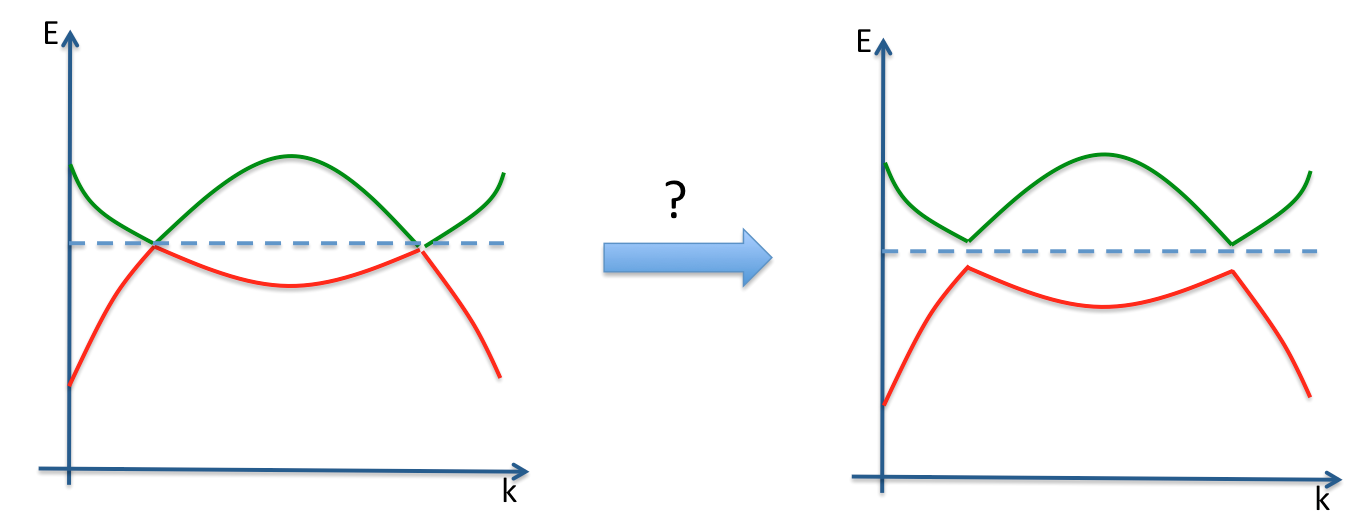
Figure 2. There are local obstructions to opening up a gap at a band crossings, related by a global consistency condition.

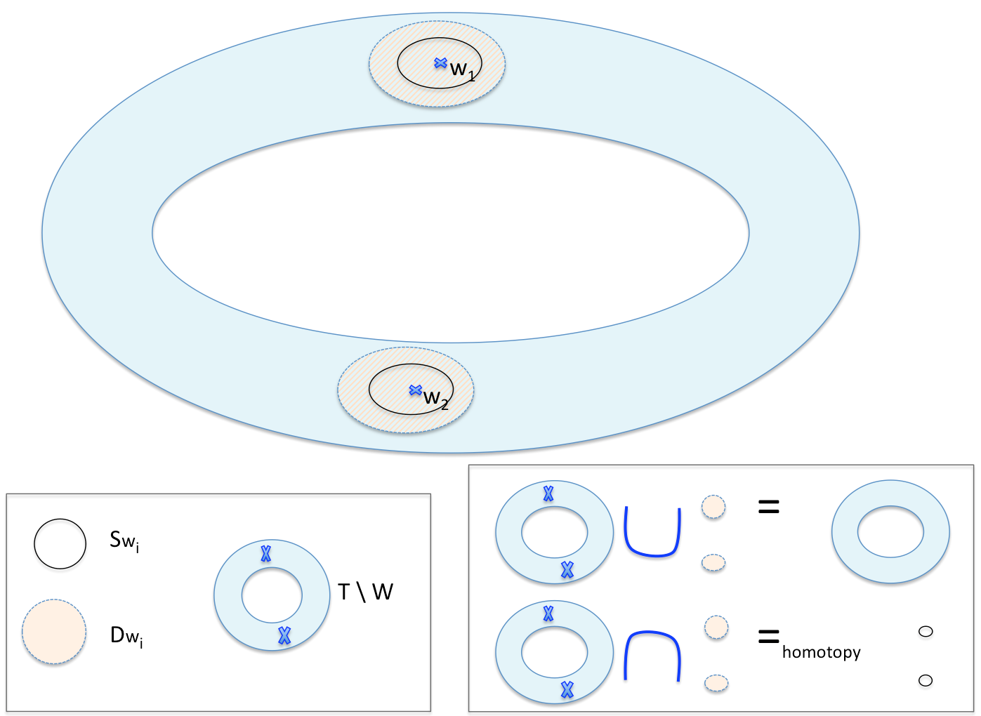
Definition of W,SW,DWW,S_{W},D_{W}. Let TT be a compact oriented dd-manifold (usually the Brillouin torus 𝕋d{\mathbb{T}}^{d} in concrete models) with d3d\geq 3, and consider a smooth family of (concrete) n×nn\times n Bloch Hamiltonians TkH(k)T\ni k\mapsto H(k). The spectrum comprises nn bands, and we assume that band crossings at the Fermi level (normalized to 00) occur on a finite set WTW\subset T of isolated “Weyl points”. On the complement TWT\setminus W, the Bloch Hamiltonians are gapped, and there is no difficulty in defining the valence bundle F\mathcal{E}_{F} over TWT\setminus W and its characteristic classes in H(TW)H^{*}(T\setminus W). For each wWw\in W, choose (mutually disjoint) open balls DwD_{w} containing ww, and (d1)(d-1)-spheres SwDwS_{w}\subset D_{w} surrounding ww. Let SW=wWSwS_{W}=\coprod_{w\in W}S_{w} and DW=wWDwD_{W}=\coprod_{w\in W}D_{w} be the respective disjoint unions. Thus TT is covered by DWD_{W} and TWT\setminus W, and the intersection of the covering sets is SW×(ϵ,ϵ)S_{W}\times(-\epsilon,\epsilon) which is homotopy equivalent to SWS_{W} (Figure 3 illustrates the setting for two Weyl points).
Refer to caption
Figure 3. Covering of TT used in the semimetal MV-sequence, for two Weyl points w1,w2w_{1},w_{2}.

The MV sequence links the cohomology groups of TT with those of the covering subspaces and the intersection SWS_{W}, by an exact sequence

H1(SW)H(T)H(TW)H(DW)H(SW)H+1(T).\cdots\rightarrow H^{*-1}(S_{W})\rightarrow H^{*}(T)\rightarrow H^{*}(T\setminus W)\oplus H^{*}(D_{W})\rightarrow H^{*}(S_{W})\rightarrow H^{*+1}(T)\rightarrow\cdots.

The maps which increase cohomological degree are the MV connecting maps, while the others are (differences of) restriction maps. Note that the H(DW)H^{*}(D_{W}) terms vanish for >0*>0 since DWD_{W} is a disjoint union of contractible sets.

When a semimetallic Bloch Hamiltonian is specified abstractly by a vector field 𝒉\bm{{h}} as in Definition 2.1, the zero set of 𝒉\bm{{h}} will correspond to the Weyl points WW, and we have the subsets SW,DWS_{W},D_{W} exactly as above. Then 𝒉\bm{{h}} defines a topological invariant for the semimetal which lives in Hd1(TW)H^{d-1}(T\setminus W) (Section 3). The most interesting part of the MV sequence is at =d1*=d-1, which we call the cohomological semimetal MV sequence,

(2.3) 0Hd1(T)(weak) insulatorιHd1(TW)insulator/semimetal𝛽Hd1(SW)local chargesΣHd(T)total charge0,\cdots 0\longrightarrow\underbrace{H^{d-1}(T)}_{\text{(weak) insulator}}\overset{\iota^{*}}{\longrightarrow}\underbrace{H^{d-1}(T\setminus W)}_{\text{insulator/semimetal}}\overset{\beta}{\longrightarrow}\underbrace{H^{d-1}(S_{W})}_{\text{local charges}}\overset{\Sigma}{\longrightarrow}\underbrace{H^{d}(T)}_{\text{total charge}}\longrightarrow 0\cdots,

Here Hd1(SW)=wWHd1(Sw)H^{d-1}(S_{W})=\oplus_{w\in W}H^{d-1}(S_{w}) is the direct sum of the local charge groups for each ww, and the last MV connecting map Σ\Sigma is the “total charge operator” which adds up the local charges [9]. For integer coefficients, Hd1(Sw)Hd(T)H^{d-1}(S_{w})\cong{\mathbb{Z}}\cong H^{d}(T) and the charges are {\mathbb{Z}}-valued, but we will also consider 2{\mathbb{Z}}_{2} coefficients in Section 5.

2.4. Basic two-band Weyl semimetal in 3D

Let us be more explicit in the basic 3D situation, with 2×22\times 2 Bloch Hamiltonians parametrised by k𝕋3k\in{\mathbb{T}}^{3} and W={w1,w2}W=\{w_{1},w_{2}\}. The MV-sequence reads

(2.4) 0H2(𝕋3)ιH2(𝕋3W)𝛽H2(Sw12Sw22)ΣH3(𝕋3)0\cdots 0\rightarrow H^{2}({\mathbb{T}}^{3})\xrightarrow{\iota^{*}}H^{2}({\mathbb{T}}^{3}\setminus W)\xrightarrow{\beta}H^{2}(S^{2}_{w_{1}}\coprod S^{2}_{w_{2}})\xrightarrow{\Sigma}H^{3}({\mathbb{T}}^{3})\rightarrow 0\ldots

Consider local charges (+q,q)H2(Sw12Sw22)(+q,-q)\in H^{2}(S^{2}_{w_{1}}\coprod S^{2}_{w_{2}}) which cancel, then there exists (by exactness) a line bundle F\mathcal{E}_{F} over 𝕋3W{\mathbb{T}}^{3}\setminus W whose restriction to SwiS_{w_{i}} has Chern class given by the local charge at wiw_{i}.

Refer to caption
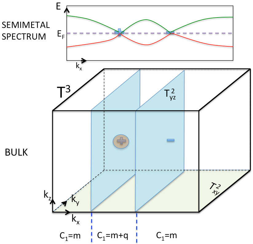
Figure 4. For each kxk_{x} away from W={+,}W=\{+,-\} (with charges (+q,q)(+q,-q)), F\mathcal{E}_{F} has a first Chern number c1(kx)c1yz(kx)c_{1}(k_{x})\equiv c_{1}^{yz}(k_{x}) on the 2D subtorus in the yy-zz direction (blue). Consider the region XX between the two blue 2-tori, with a small ball around ++ removed. This is a 3-manifold whose boundary X\partial X consists of the two blue 2-tori (oppositely oriented) together with a small 2-sphere around ++. Note that the top and bottom faces are identified, as are the front and back faces so they do not contribute to X\partial X. Everywhere on XX, the valence line bundle is well-defined, and its Berry curvature 2-form \mathcal{F} is closed. By Stokes’ theorem, 0=Xd=X0=\int_{X}\text{d}\mathcal{F}=\int_{\partial X}\mathcal{F}, so the difference between the first Chern numbers for the left 2-torus and the right 2-torus is precisely the first Chern number on the small 2-sphere, which is +q+q. This argument is easily generalised to higher dimensions and higher curvature forms (Remark 3.7).

Intuitive idea behind relation between local charges and first Chern numbers of a Weyl semimetal. Suppose the vector field 𝒉\bm{{h}} on 𝕋3{\mathbb{T}}^{3} vanishes at w1,w2w_{1},w_{2} with local indices +q,q+q,-q respectively. For simplicity, we first assume that wiw_{i} have the same ky,kzk_{y},k_{z}-coordinates, as in Figure 4. Take a trivial Bloch bundle 𝒮0=𝕋3×2\mathscr{S}_{0}={\mathbb{T}}^{3}\times{\mathbb{C}}^{2}, the Pauli matrices σ1,σ2,σ3\sigma_{1},\sigma_{2},\sigma_{3} with respect to a trivialisation, and let H(k)=𝒉(k)𝝈H(k)=\bm{{h}}(k)\cdot\bm{{\sigma}}. Then on 𝕋3W{\mathbb{T}}^{3}\setminus W, the valence line bundle F\mathcal{E}_{F} is well-defined. At each kxk_{x} away from the Weyl points, F\mathcal{E}_{F} has first Chern numbers c1yz(kx)c_{1}^{yz}(k_{x}) obtained by pairing c1(F)c_{1}(\mathcal{E}_{F}) with the fundamental class of the 2-torus at kxk_{x} (integrating the Berry curvature over the 2-torus). The integer c1yzc_{1}^{yz} is sometimes called a “weak invariant” for “weak” topological insulators supported on lower-dimensional subtori of the Brillouin torus. As a function of kxk_{x}, c1yzc_{1}^{yz} remains constant unless a Weyl point is traversed, whence it jumps by an amount equal to the local charge there. A possible function c1yzc_{1}^{yz} is given at the bottom of Figure 4, and different choices of 𝒉\bm{{h}} can give rise to different mm.

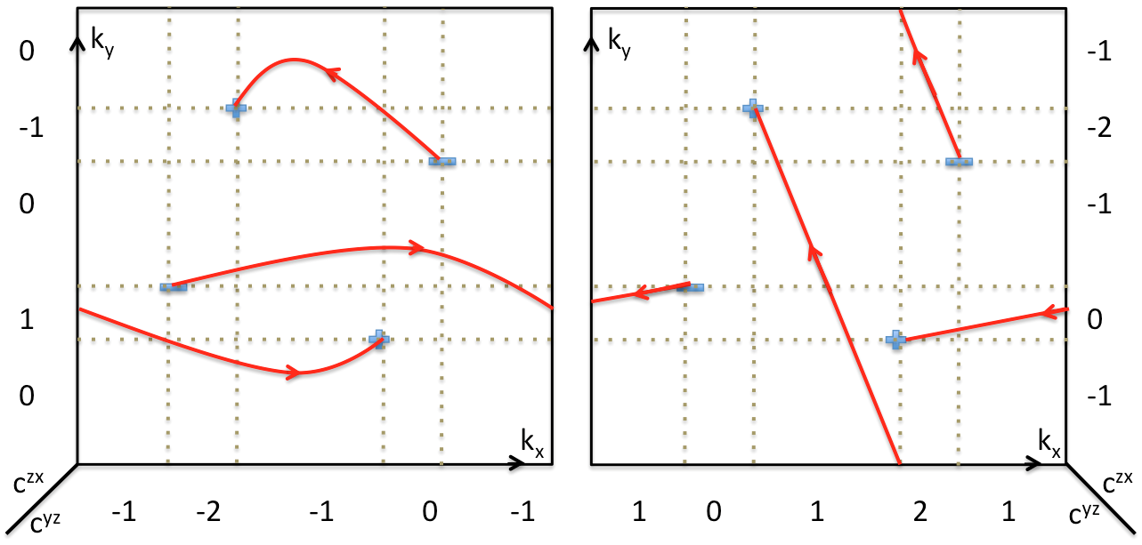
Note that even with mm and the local charges ±q\pm q still do not completely specify the class of F\mathcal{E}_{F} — there are two other independent first Chern numbers c1xy,c1zxc_{1}^{xy},c_{1}^{zx} which are constant functions of kzk_{z} and kyk_{y} respectively (since both Weyl points are traversed simultaneously as either kzk_{z} or kyk_{y} is varied). In general, the wiw_{i} need not have the same ky,kzk_{y},k_{z}-coordinates, and so there are similar jumps in the functions c1xy(kz)c_{1}^{xy}(k_{z}) and c1zx(ky)c_{1}^{zx}(k_{y}), see Figures 11-12. There is a simple way to concisely and invariantly (i.e. coordinate-free) capture all the jumps in the various first Chern numbers, through a Poincaré dual picture in terms of Euler chains (see Section 3.4 and Remark 3.7).

All first Chern numbers can appear in a Weyl semimetal. Let us also consider F\mathcal{E}^{\prime}_{F} which arise as a subbundle of a possibly non-trivial Bloch bundle 𝒮\mathscr{S}. Such F\mathcal{E}^{\prime}_{F} are easily obtained by tensoring 𝒮0\mathscr{S}_{0} with a line bundle \mathcal{L} with c1()H2(𝕋3)c_{1}(\mathcal{L})\in H^{2}({\mathbb{T}}^{3}). The “twisted” Hamiltonian H(k)=(𝒉(k)𝝈)1H^{\prime}(k)=(\bm{{h}}(k)\cdot\bm{{\sigma}})\otimes 1 acts on the “twisted” Bloch bundle 𝒮=𝒮0\mathscr{S}=\mathscr{S}_{0}\otimes\mathcal{L}, and has valence line bundle F=F\mathcal{E}^{\prime}_{F}=\mathcal{E}_{F}\otimes\mathcal{L} (defined over 𝕋3W{\mathbb{T}}^{3}\setminus W). Therefore c1(F)=c1(F)+ι(c1())c_{1}(\mathcal{E}^{\prime}_{F})=c_{1}(\mathcal{E}_{F})+\iota^{*}(c_{1}(\mathcal{L})) and, in particular, the first Chern numbers c1yz(F)c_{1}^{yz}(\mathcal{E}^{\prime}_{F}) increases by c1yz()c_{1}^{yz}(\mathcal{L}) and similarly for c1xy,c2zxc_{1}^{xy},c_{2}^{zx}. In this way, all elements of H2(𝕋3W)H^{2}({\mathbb{T}}^{3}\setminus W) can be realised as valence line bundles of some semimetallic Bloch Hamiltonian.

2.5. Geometric interpretation of MV sequence

In d=3d=3, the exact sequence (2.3) has a direct interpretation as a solution to a geometrical extension problem, which we can interpret in terms of insulator-semimetal transitions. Let us recall that H2(T,)H^{2}(T,{\mathbb{Z}}) classifies line bundles over TT (e.g. determinant valence bundles). So for T=𝕋3T={\mathbb{T}}^{3}, the exactness of (2.3) tells us the following:

  1. (1)

    A collection of line bundles wSw\mathcal{L}_{w}\rightarrow S_{w} with Chern classes cwc_{w} may be extended to a line bundle over TWT\setminus W (comes from a semimetal) iff wWcw=0\sum_{w\in W}c_{w}=0 (local charges cancel).

  2. (2)

    A line bundle TW\mathcal{L}\rightarrow T\setminus W extends to all of TT iff each local charge vanishes. Thus a semimetal (whose valence bundle represents a class in H2(TW)H^{2}(T\setminus W)) can be gapped into an insulator iff all the local charges are zero. A topological semimetal with a topologically protected crossing at ww has non-zero local charge there.

  3. (3)

    The insulator invariants in H2(T)H^{2}(T) (“weak” Chern insulators) appear faithfully in H2(TW)H^{2}(T\setminus W). Thus two semimetals with the same local charge (same image under β\beta) can be globally inequivalent, differing by some element in (the image under ι\iota^{*} of) H2(T)H^{2}(T) (the weak invariants).

An important consequence of Point 3 is that the local charge information is not sufficient to determine the global band structure of the semimetal. As explained in [41], this ambiguity has crucial consequences for the determination of the resulting surface Fermi arcs. We will have more to say about this in Section 3.4.2, see also Figure 10.

More generally, in d3d\geq 3, a Dirac-type Bloch Hamiltonian in the sense of Definition 2.1 determines by restriction smooth maps 𝒉^w:SwSd1,wW\hat{\bm{{h}}}_{w}:S_{w}\longrightarrow S^{d-1},w\in W, and the semimetal MV sequence can be interpreted at this level. In Appendix A we describe the relevant geometric structures on Sd1S^{d-1}, d=3,4,5d=3,4,5, and these can be pulled back to SWS_{W} via all the 𝒉^w\hat{\bm{{h}}}_{w}.

  1. (1)

    In d=3d=3, let \mathcal{L} be the Hopf line bundle over S2S^{2}. Consider a collection of pullback line bundles 𝒉^w()\hat{\bm{{h}}}_{w}^{*}(\mathcal{L}) over SwS_{w}, such that wWc1(𝒉^w())=0=wWdeg(𝒉^w)\sum_{w\in W}c_{1}(\hat{\bm{{h}}}_{w}^{*}(\mathcal{L}))=0=\sum_{w\in W}\deg(\hat{\bm{{h}}}_{w}), where deg(𝒉^w)\deg(\hat{\bm{{h}}}_{w}) denotes the degree of the map 𝒉^w\hat{\bm{{h}}}_{w}. Although they individually may not extend to T{w}T\setminus\{w\}, together wW𝒉^w()\coprod_{w\in W}\hat{\bm{{h}}}_{w}^{*}(\mathcal{L}) over SWS_{W} does extend to TWT\setminus W by exactness of the MV sequence. See the Appendix for more information.

  2. (2)

    In d=4d=4, the H3H^{3} part of the semimetal Mayer–Vietoris sequence

    (2.5) 0H3(T)ιH3(TW)𝛽H3(SW3)ΣH4(T)0\cdots 0\rightarrow H^{3}(T)\xrightarrow{\iota^{*}}H^{3}(T\setminus W)\xrightarrow{\beta}H^{3}(S^{3}_{W})\xrightarrow{\Sigma}H^{4}(T)\rightarrow 0\ldots

    has the following analogous geometric interpretation. We refer the reader to Appendix A for a primer on gerbes and the construction of the basic gerbe on SU(2)\text{SU}(2). A collection of pullback basic gerbes 𝒢wSw\mathcal{G}_{w}\rightarrow S_{w} with Dixmier–Douady numbers DDwDD_{w} may be extended to a gerbe over TWT\setminus W (comes from a gerbe semimetal) iff wWDDw=0\sum_{w\in W}DD_{w}=0 (local DD charges cancel). The pullback basic gerbe 𝒢TW\mathcal{G}\rightarrow T\setminus W extends to all of TT iff each local DD charge vanishes. Thus a gerbe semimetal (with topological invariant in H3(TW)H^{3}(T\setminus W)) can be gapped into an insulator iff all the local DD charges are zero. A topological gerbe semimetal with a topologically protected crossing at ww has non-zero local DD charge there. The insulator invariants in H3(T)H^{3}(T) (“weak” gerbe insulators) appear faithfully in H3(TW)H^{3}(T\setminus W). Thus two gerbe semimetals with the same local DD charge (same image under β\beta) can be globally inequivalent, differing by some element in (the image under ι\iota^{*} of) H3(T)H^{3}(T). Conversely, the pullback gerbes 𝒉^w(𝒢)\hat{\bm{{h}}}_{w}^{*}(\mathcal{G}) over SwS_{w}, where 𝒢\mathcal{G} is the basic gerbe over S3SU(2)S^{3}\cong\text{SU}(2), such that wWDD(𝒉^w(𝒢))=0=wWdeg(𝒉^w)\sum_{w\in W}DD(\hat{\bm{{h}}}_{w}^{*}(\mathcal{G}))=0=\sum_{w\in W}\deg(\hat{\bm{{h}}}_{w}). Although the 𝒉^w(𝒢)\hat{\bm{{h}}}_{w}^{*}(\mathcal{G}) may not individually extend to T{w}T\setminus\{w\}, the gerbe wW𝒉^w(𝒢)\coprod_{w\in W}\hat{\bm{{h}}}_{w}^{*}(\mathcal{G}) does extend to TWT\setminus W by exactness of the MV sequence. See Section 4.6.1 and the Appendix for more details.

  3. (3)

    In d=5d=5, the analysis is analogous to the case of line bundles done above. One replaces the line bundle \mathcal{L} over 1{\mathbb{C}}{\mathbb{P}}^{1} by the quaternionic line bundle \mathcal{H} over 1{\mathbb{H}}{\mathbb{P}}^{1} and one uses the MV sequence in (4.3), where the first Chern class is replaced by the 2nd Chern class. See Section 4.5 and the Appendix for more details.

Although there is a MV sequence analysis in the case of Kervaire semimetals (Section 5.4), we are unable to formulate a geometric extension problem in this context (see Section 6).

2.5.1. Adiabatic connections

In Section 2.1, we briefly alluded to the relation between Chern numbers and Berry connections associated to valence subbundles for a family of Hamiltonians over TT. In general, a rank-nn eigen-subbundle has a U(n)\text{U}(n) adiabatic (non-abelian Berry) connection, whose curvature gives the real (de Rham) Chern classes of the subbundle [55]. For n=1n=1, the curvature 2-form is involved in computing first Chern numbers. In the presence of time-reversal symmetry, the subbundle is complex even-dimensional and in fact a quaternionic symplectic bundle with quaternionic dimension m=n2m=\frac{n}{2}; the Berry connection becomes a Sp(m)\text{Sp}(m) one, see [5, 6, 23] and Section 4.5.2. For m=1m=1, the 4-form obtained from squaring the curvature enters in the computation of second Chern numbers. In a similar vein, the additional imposition of a chiral symmetry allows a “semimetal gerbe” to be associated to the family of Hamiltonians, see Section 4.6.1. There is a “Berry connection 2-form” with 3-form curvature, which computes the Dixmier–Douady invariants of the gerbe.

2.6. Dual MV sequence and Fermi arcs

Fermi arcs are more naturally analyzed in homology, and for this reason, we Poincaré-dualise (2.3)

(2.6) 0H1(T)Euler structuresH1(T,W)Euler chainsH0(SW)H0(W)local chargesH0(T)total charge0,\cdots 0\rightarrow\underbrace{H_{1}(T)}_{\text{Euler structures}}\rightarrow\underbrace{H_{1}(T,W)}_{\text{Euler chains}}\overset{\partial}{\rightarrow}\underbrace{H_{0}(S_{W})\cong H_{0}(W)}_{\text{local charges}}\rightarrow\underbrace{H_{0}(T)}_{\text{total charge}}\rightarrow 0\cdots,

with the physical meanings of the first two groups explained in Section 3. Roughly speaking, the Poincaré dual of a semimetal invariant in H2(TW)H^{2}(T\setminus W) is an Euler chain in the relative homology group H1(T,W)H_{1}(T,W), whose boundary is the 0-chain of local charge data.

Equation (2.6) can also be exhibited directly as a Mayer–Vietoris sequence for Borel–Moore homology HBMH^{\text{BM}}_{*} [8, 27]. The groups HBM()H^{\text{BM}}_{*}(\cdot) may be defined for locally compact spaces XX using locally finite chains. For compact spaces, HBMH^{\text{BM}}_{*} and the usual (singular) homology HH_{*} coincide. However, H0BM(Dw)=0H^{\text{BM}}_{0}(D_{w})=0 whereas H0(Dw)H_{0}(D_{w})\cong{\mathbb{Z}}, for DwD_{w} an open ball containing ww. There are isomorphisms H1(T,W)H1BM(TW)H_{1}(T,W)\cong H^{\text{BM}}_{1}(T\setminus W), H(X)H+1BM(X×)H_{*}(X)\cong H^{\text{BM}}_{*+1}(X\times{\mathbb{R}}), Poincaré duality Hd1(T)H1BM(TW)H^{d-1}(T)\cong H^{\text{BM}}_{1}(T\setminus W), and restriction maps to HBMH^{\text{BM}}_{*} of open subsets, see Chapter 2.6 of [13]. The Poincaré dual of (2.3) written in terms of HBMH^{\text{BM}}_{*} is

(2.7) 0H1BM(T)H1BM(TW)H1BM(SW×(ϵ,ϵ))H0BM(T)0,\cdots 0\longrightarrow H^{\text{BM}}_{1}(T)\longrightarrow H^{\text{BM}}_{1}(T\setminus W)\longrightarrow H^{\text{BM}}_{1}(S_{W}\times(-\epsilon,\epsilon))\longrightarrow H^{\text{BM}}_{0}(T)\longrightarrow 0\cdots,

which is precisely the MV-sequence for HBMH^{\text{BM}}_{*} (IX.2.3 of [27]), with respect to the open cover {DW,TW}\{D_{W},T\setminus W\} of TT; c.f. the “localization” long exact sequence, IX.2.1 of [27] and 2.6.10 of [13]. The sequences (2.7) and (2.6) are the same on account of H1BM(SW×(ϵ,ϵ))H0(SW)H^{\text{BM}}_{1}(S_{W}\times(-\epsilon,\epsilon))\cong H_{0}(S_{W}). The language of Borel–Moore homology has certain advantages, but for this paper we stay in the more elementary setting of relative homology so as to avoid having to introduce too much technical machinery.

In [41], we explained how Fermi arcs represent relative homology classes in H1(T~,W~)H_{1}(\widetilde{T},\widetilde{W}), where π:(T,W)(T~,W~)\pi:(T,W)\rightarrow(\widetilde{T},\widetilde{W}) projects out one torus direction, so T~\widetilde{T} is the surface Brillouin zone. The Euler chain representing the topological data of a semimetal is projected onto a surface Fermi arc, and this is the Poincaré dual picture of the bulk-boundary correspondence, see Section 3.4.2.

3. Euler chains and semimetal Hamiltonians

Since we parametrise Dirac-type Bloch Hamiltonians by vector fields 𝒉\bm{{h}} on TT, we would also like to analyse the semimetal MV-sequence (2.3) in terms 𝒉\bm{{h}} and its homotopies. In the insulating case, we might want to maintain the gap condition and so consider homotopies through non-singular (i.e. nowhere vanishing) vector fields. In the semimetal case, we want to at least maintain the gap condition everywhere except perhaps at a finite set of isolated Weyl points. We may require the set of Weyl points and their charges to be kept fixed, or we may allow them to move around and be created/annihilated in pairs. In Section 3.1, we explain why it is important to keep track of the “history” of the creation/annihilation of Weyl points as part of the topological data of a semimetal band structure. This motivates the mathematical notion of Euler structures, which we introduce in Section 3.2, as well as the dual notion of Euler chains for keeping track of Weyl point connectivity, introduced in Section 3.3. The Euler chain representation of a semimetal is then explained in Section 3.4.

3.1. Weyl pair creation and annihilation

Heuristically, a pair of Weyl points with opposite charges +1+1 and 1-1 may be created at a particular point in TT where a valence and conduction band cross. Then the Weyl points are moved apart in TT to form two separate band crossings, each of which is topologically protected and cannot be gapped out. In the reverse direction, if two separate Weyl points with opposite charges come together at a single point, their charges annihilate and a gap can be opened at that point. What is particularly interesting is that a TT with some non-trivial 1-cycle (such as T=𝕋3T={\mathbb{T}}^{3}) admits a scenario in which a pair of of Weyl points is created at a single point, moved apart in opposite directions along the 1-cycle, and then annihilated when they meet again. This creation/annihilation process is global, and the history traces out the 1-cycle (Fig. 5-6).

Refer to caption
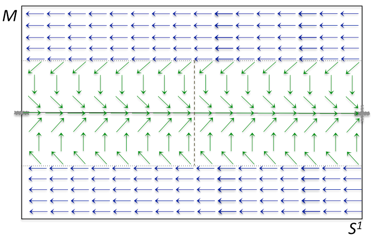
Figure 5. A typical way to locally introduce a pair of opposite-degree zeroes into a vector field. Here, the compact oriented dd-manifold TT is S1×MS^{1}\times M, and we perturb an initial global non-vanishing vector field (blue) by modifying it within a ball containing the desired zeroes (black ±\pm symbols). The region enclosed by the dotted line is a tubular neighbourhood to the open black line connecting - to ++, so that each cross-section (dashed line) is an open ball Dd1D^{d-1} in MM. For each cross-section, we assign tangent directions (green arrows, elements of Sd1S^{d-1}) to the closed ball D¯d1\overline{D}^{d-1} by the surjective map D¯d1Sd1\overline{D}^{d-1}\rightarrow S^{d-1} which collapses D¯d1\partial\overline{D}^{d-1} to the point corresponding to the blue arrow. On a small d1d-1-sphere S±d1S^{d-1}_{\pm} surrounding ±\pm, the assignment of tangent directions is a degree ±1\pm 1 map S±d1Sd1S^{d-1}_{\pm}\rightarrow S^{d-1} as required. This is essentially the Pontryagin–Thom construction, see [43].
Refer to caption
Figure 6. If the locally created zeroes of Fig. 5 are moved apart in opposite directions along the cycle S1S^{1}, and then annihilated when they meet (grey ±\pm symbols), the result is a global vector field modified (as in the green arrows) from the initial one (blue arrows) within a tubular neighbourhood S1×Dd1S^{1}\times D^{d-1} to the trajectory of the zeroes.

Even though both the initial and final band structures have no band crossings, they can generally become topologically inequivalent during this process. For example, take T=𝕋3T={\mathbb{T}}^{3} (so M=𝕋2M={\mathbb{T}}^{2}) in Fig. 5-6. The initial constant vector field 𝒉\bm{{h}} over 𝕋3{\mathbb{T}}^{3} corresponds to an initial gapped Hamiltonian HH with trivial valence band 𝒉^()\hat{\bm{{h}}}^{*}(\mathcal{L}), where \mathcal{L} is the Hopf line bundle over S21S^{2}\cong{\mathbb{C}}{\mathbb{P}}^{1} as in Sec. 2.5. On the other hand, the final vector field 𝒉\bm{{h}}^{\prime} is such that the unit vector map 𝒉^:𝕋3S2\hat{\bm{{h}}^{\prime}}:{\mathbb{T}}^{3}\rightarrow S^{2} restricts to a degree-1 map 𝕋2S2{\mathbb{T}}^{2}\rightarrow S^{2} on each cross-section 𝕋2{\mathbb{T}}^{2} to the Weyl points’ trajectory S1S^{1}. Thus the valence band of the final gapped Hamiltonian HH^{\prime}, which is 𝒉^()\hat{\bm{{h}}^{\prime}}^{*}(\mathcal{L}), “acquires” a weak Chern class supported in the 𝕋2{\mathbb{T}}^{2} directions (which is Poincaré dual to S1S^{1}). We learn that a local Weyl point creation-annihilation process does not change the weak invariants of a Hamiltonian, but a global one can. This motivates, and provides a physical interpretation of, a certain notion of equivalence of vector fields (thus of Hamiltonians) defined formally in the next subsection.

3.2. Euler structures

Smooth Euler structures. Let TT be a compact oriented dd-manifold with d2d\geq 2, and suppose TT has Euler characteristic χ(T)=0\chi(T)=0 (this is automatic in d=3d=3) so that it has a global non-vanishing vector field.

Definition 3.1 ([65]).

Two non-singular smooth vector fields 𝒉,𝒉\bm{{h}},\bm{{h}}^{\prime} on TT are said to be homotopic (also called homologous33 3 The stronger notion of homotopy on TT through non-singular vector fields can also be analysed [65], but we do not consider this in this paper. in [65]) if for some open ball DD, the fields 𝒉,𝒉\bm{{h}},\bm{{h}}^{\prime} are homotopic on TDT\setminus D in the class of non-singular vector fields on TDT\setminus D. The set 𝔳𝔢𝔠𝔱(T)\mathfrak{vect}(T) of homotopy classes of non-singular vector fields is called the set of smooth Euler structures on TT.

As explained in Section 5 of [65], the first obstruction to such a homotopy between 𝒉,𝒉\bm{{h}},\bm{{h}}^{\prime} is an element (written as 𝒉/𝒉\bm{{h}}/\bm{{h}}^{\prime}) of Hd1(T,πd1(Sd1))Hd1(T,)H^{d-1}(T,\pi_{d-1}(S^{d-1}))\cong H^{d-1}(T,{\mathbb{Z}}), canonically isomorphic to H1(T,)H_{1}(T,{\mathbb{Z}}) by Poincaré duality. It turns out that there is a natural free and transitive action of the group of obstructions Hd1(T,)H1(T,)H^{d-1}(T,{\mathbb{Z}})\cong H_{1}(T,{\mathbb{Z}}) on 𝔳𝔢𝔠𝔱(T)\mathfrak{vect}(T).

Remark 3.1.

If we pick a reference nonsingular 𝒉ref\bm{{h}}_{\text{ref}} as the zero, then we can identify 𝔳𝔢𝔠𝔱(T)\mathfrak{vect}(T) with Hd1(T,)H^{d-1}(T,{\mathbb{Z}}). For T=𝕋dT={\mathbb{T}}^{d}, a natural choice for 𝒉ref\bm{{h}}_{\text{ref}} is a constant length vector field pointing along a torus cycle (this gives a trivial insulating phase); reference to such a 𝒉ref\bm{{h}}_{\text{ref}} will be implicit in this case. We remark that the space of spinc structures for TT is a H2(T,)H^{2}(T,{\mathbb{Z}})-torsor, and that when d=3d=3, a non-singular 𝒉ref\bm{{h}}_{\text{ref}} determines a spinc structure through the unit vector field 𝒉^ref\hat{\bm{{h}}}_{\text{ref}} [66], and vice-versa.

3.2.1. Another picture of Euler structures

An equivalent definition of Euler structures, which is useful for our generalisation to Kervaire structures in Section 5.4, was given in [66] as follows.

Definition 3.2.

Let TT be a compact oriented dd-manifold with χ(T)=0\chi(T)=0, and let 𝒮𝒮()\mathcal{S}\equiv\mathcal{S}(\mathcal{E}) be the unit sphere bundle for the tangent bundle T\mathcal{E}\rightarrow T (with a Riemannian metric). Define the set of Euler structures to be the subset 𝔠𝔬𝔈𝔲𝔩~(T)Hd1(𝒮,)\widetilde{\mathfrak{coEul}}(T)\subset H^{d-1}(\mathcal{S},{\mathbb{Z}}) for which the restriction to each (oriented) fibre 𝒮kSd1\mathcal{S}_{k}\cong S^{d-1} generates Hd1(Sd1,)H^{d-1}(S^{d-1},{\mathbb{Z}}).

Then there is a free and transitive action of H1(T,)Hd1(T,)H_{1}(T,{\mathbb{Z}})\cong H^{d-1}(T,{\mathbb{Z}}) on 𝔠𝔬𝔈𝔲𝔩~(T)\widetilde{\mathfrak{coEul}}(T) under pullback to 𝒮\mathcal{S} and addition in Hd1(𝒮,)H^{d-1}(\mathcal{S},{\mathbb{Z}}). To pass from the first picture of smooth Euler structures as 𝔳𝔢𝔠𝔱(T)\mathfrak{vect}(T) to this second picture, notice that the unit vector field 𝒉^\hat{\bm{{h}}} for a non-singular 𝒉\bm{{h}} is a map T𝒮T\rightarrow\mathcal{S} and so a dd-cycle in 𝒮\mathcal{S}. Orient 𝒮\mathcal{S} by requiring the intersection number of every 𝒮k\mathcal{S}_{k} with this cycle to be +1+1. Then the dd-cycle 𝒉^\hat{\bm{{h}}} Poincaré dualises to a (d1)(d-1)-cocycle which we write as PD𝒉\text{PD}_{\bm{{h}}}, and the latter represents an Euler structure in 𝔠𝔬𝔈𝔲𝔩~(T)Hd1(𝒮,)\widetilde{\mathfrak{coEul}}(T)\subset H^{d-1}(\mathcal{S},{\mathbb{Z}}) in the second picture. To emphasize the cohomology definition of Euler structure, we will sometimes use the term co-Euler structure, to distinguish it from a homological definition to be given in Section 3.3.

As with 𝔳𝔢𝔠𝔱(T)\mathfrak{vect}(T), there is an identification of the affine space 𝔠𝔬𝔈𝔲𝔩~(T)\widetilde{\mathfrak{coEul}}(T) with Hd1(T,)H^{d-1}(T,{\mathbb{Z}}) upon fixing a reference non-singular 𝒉ref\bm{{h}}_{\text{ref}}. Writing p:𝒮Tp:\mathcal{S}\rightarrow T for the projection, we note that 𝒉^refp=id\hat{\bm{{h}}}_{\text{ref}}^{*}\circ p^{*}=\text{id} in the Gysin sequence

(3.1) 0Hd1(T,)𝒉^refpHd1(𝒮,)pH0(T,)0,0\longrightarrow H^{d-1}(T,{\mathbb{Z}})\overset{p^{*}}{\underset{\hat{\bm{{h}}}_{\text{ref}}^{*}}{\rightleftarrows}}H^{d-1}(\mathcal{S},{\mathbb{Z}})\overset{p_{*}}{\longrightarrow}H^{0}(T,{\mathbb{Z}})\longrightarrow 0,

with pp_{*} the pushforward, or integration over the Sd1S^{d-1} fibers.

The subset 𝔠𝔬𝔈𝔲𝔩~(T)Hd1(𝒮,)\widetilde{\mathfrak{coEul}}(T)\subset H^{d-1}(\mathcal{S},{\mathbb{Z}}) comprises [PD𝒉ref][\text{PD}_{\bm{{h}}_{\text{ref}}}] and all its translates by p(Hd1(T,))p^{*}(H^{d-1}(T,{\mathbb{Z}})), so 𝒉^ref\hat{\bm{{h}}}_{\text{ref}}^{*} gives a bijection from 𝔠𝔬𝔈𝔲𝔩~(T)Hd1(T,)\widetilde{\mathfrak{coEul}}(T)\rightarrow H^{d-1}(T,{\mathbb{Z}}) taking [PD𝒉ref][\text{PD}_{\bm{{h}}_{\text{ref}}}] to the identity element.

3.3. Euler chains and singular vector fields

There is a dual picture of Euler structures involving vector fields with finite singularities, which is closely related to the intuition behind Fermi arcs. We sketch the construction here for the case of non-degenerate zeroes, see [26, 12, 44] for the general case.

For a vector field 𝒉\bm{{h}} on TT with finite singularity set W𝒉W_{\bm{{h}}}, let 𝒲𝒉\mathcal{W}_{\bm{{h}}} denote the singular 0-chain 𝒲𝒉wW𝒉Indw(𝒉)wC0(T,)\mathcal{W}_{\bm{{h}}}\coloneqq\sum_{w\in W_{\bm{{h}}}}\text{Ind}_{w}(\bm{{h}})w\in C_{0}(T,{\mathbb{Z}}) which encodes the local charge information. We can also think of 𝒲𝒉\mathcal{W}_{\bm{{h}}} as an element of H0(W𝒉,)H_{0}(W_{\bm{{h}}},{\mathbb{Z}}) whose weights sum to zero.

Definition 3.3 ([26]).

Let TT be a compact dd-manifold with d2d\geq 2 and χ(T)=0\chi(T)=0. An Euler chain for a 0-chain 𝒲\mathcal{W} in TT whose weights sum to zero, is a 1-chain lC1(T,)l\in C_{1}(T,{\mathbb{Z}}) such that l\partial l is 𝒲\mathcal{W}. An Euler chain ll defines a relative homology class in H1(T,W,)H_{1}(T,W,{\mathbb{Z}}) where WW is the set of points that 𝒲\mathcal{W} is defined on44 4 𝒲\mathcal{W} is allowed to be zero on points in WW.. Let 𝔈𝔲𝔩(T,𝒲)H1(T,W,)\mathfrak{Eul}(T,\mathcal{W})\subset H_{1}(T,W,{\mathbb{Z}}) denote the subset of relative homology classes of 1-chains in TT whose boundary is 𝒲\mathcal{W}.

From the exact sequence

0=H1(W,)H1(T,)H1(T,W,)H0(W,)ΣH0(T,)H0(T,W,)=0,0=H_{1}(W,{\mathbb{Z}})\rightarrow H_{1}(T,{\mathbb{Z}})\rightarrow H_{1}(T,W,{\mathbb{Z}})\overset{\partial}{\rightarrow}H_{0}(W,{\mathbb{Z}})\overset{\Sigma}{\rightarrow}H_{0}(T,{\mathbb{Z}})\rightarrow H_{0}(T,W,{\mathbb{Z}})=0,

we see that 𝔈𝔲𝔩(T,𝒲)\mathfrak{Eul}(T,\mathcal{W}) is a coset of H1(T,)H_{1}(T,{\mathbb{Z}}) in H1(T,W,)H_{1}(T,W,{\mathbb{Z}}) and so an affine space for H1(T,)H_{1}(T,{\mathbb{Z}}). In particular, the difference of [l],[l]𝔈𝔲𝔩(T,𝒲)[l],[l^{\prime}]\in\mathfrak{Eul}(T,\mathcal{W}) is an element of H1(T,)H_{1}(T,{\mathbb{Z}}). Note that any 0-chain 𝒲\mathcal{W} with total weight zero can be realised as the 0-chain of charges 𝒲𝒉\mathcal{W}_{\bm{{h}}} for some singular vector field 𝒉\bm{{h}}, by the (converse of the) Poincaré–Hopf theorem. Euler chains can be thought of as extra global data encoding how the local charge configuration for a singular vector field is “connected”. As explained in Section 3.4, Euler chains are in a precise sense Poincaré dual to cohomological semimetal invariants.

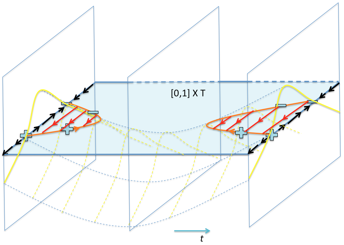
Non-degenerate homotopies. Let 𝒉,𝒉\bm{{h}},\bm{{h}}^{\prime} be two smooth vector fields, then there is a canonical identification of 𝔈𝔲𝔩(T,𝒲𝒉)\mathfrak{Eul}(T,\mathcal{W}_{\bm{{h}}}) and 𝔈𝔲𝔩(T,𝒲𝒉)\mathfrak{Eul}(T,\mathcal{W}_{\bm{{h}}^{\prime}}) as affine spaces, using a notion of non-degenerate homotopy defined as follows. Let pp^{*}\mathcal{E} be the pullback of the tangent bundle T\mathcal{E}\rightarrow T under the projection p:[0,1]×TTp:[0,1]\times T\rightarrow T. A non-degenerate homotopy between 𝒉\bm{{h}} and 𝒉\bm{{h}}^{\prime} is a section 𝒉˘\breve{\bm{{h}}} of pp^{*}\mathcal{E} transverse to the zero section, which restricts to 𝒉\bm{{h}} at t=0t=0 and 𝒉\bm{{h}}^{\prime} at t=1t=1. Such a homotopy exists by perturbing, for instance, a linear homotopy, and allows for the movement tW𝒉tt\mapsto W_{\bm{{h}}_{t}} of the local charges W𝒉t𝒉t1{0}W_{\bm{{h}}_{t}}\coloneqq\bm{{h}}_{t}^{-1}\{0\} including the creation and annihilation of pairs of zeros with equal and opposite charges (Fig. 7). For generic tt, the intermediate vector field 𝒉t\bm{{h}}_{t} intersects the zero vector field transversally (e.g. transversality of 𝒉t\bm{{h}}_{t} fails when a pair of Weyl points are created or annihilated). The zero set 𝒲˘\breve{\mathcal{W}} of 𝒉˘\breve{\bm{{h}}} is a canonically oriented 1-submanifold with boundary 𝒲𝒉(1)𝒲𝒉(0)\mathcal{W}_{\bm{{h}}^{\prime}}^{(1)}-\mathcal{W}_{\bm{{h}}}^{(0)}, where the superscript indicates whether the 0-chain lies on {0}×T\{0\}\times T or on {1}×T\{1\}\times T. Let [l]𝔈𝔲𝔩(T,𝒲𝒉)[l]\in\mathfrak{Eul}(T,\mathcal{W}_{\bm{{h}}}), then 𝒲˘+l\breve{\mathcal{W}}+l is a 1-cycle on [0,1]×T[0,1]\times T relative to {1}×T\{1\}\times T, since (𝒲˘+l)=𝒲𝒉(1)\partial(\breve{\mathcal{W}}+l)=\mathcal{W}_{\bm{{h}}^{\prime}}^{(1)}. Because H1([0,1]×T,{1}×T)=0H_{1}([0,1]\times T,\{1\}\times T)=0, there is a 2-chain PP on [0,1]×T[0,1]\times T whose boundary is 𝒲˘+l\breve{\mathcal{W}}+l relative to {1}×T\{1\}\times T. Taking l𝒲˘+lPl^{\prime}\coloneqq\breve{\mathcal{W}}+l-\partial P, we see that ll^{\prime} is a 1-chain on {1}×T\{1\}\times T with l=𝒲𝒉(1)\partial l^{\prime}=\mathcal{W}_{\bm{{h}}^{\prime}}^{(1)}, which defines a class [l]𝔈𝔲𝔩(T,𝒲𝒉)[l^{\prime}]\in\mathfrak{Eul}(T,\mathcal{W}_{\bm{{h}}^{\prime}}). Intuitively, we can think a homotopy 𝒉˘\breve{\bm{{h}}} as providing the data of how an initial ll is to be “carried along 𝒲˘\breve{\mathcal{W}}” onto a final ll^{\prime}.

Refer to caption
Figure 7. The homotopy parameter t[0,1]t\in[0,1] goes horizontally, while all coordinates for the manifold TT are suppressed except one cyclic S1S^{1}-direction. The height function at each tt (yellow curve) indicates the length of a tangent vector on {t}×T\{t\}\times T in the aforementioned direction. Black arrows represent one component of the initial (left) vector field 𝒉\bm{{h}} and final (right) one 𝒉\bm{{h}}^{\prime}, which are taken to be equal in this example. The zero-section of the tangent bundle of [0,1]×T[0,1]\times T is the blue shaded area. A non-degenerate homotopy 𝒉˘\breve{\bm{{h}}} is shown, with the intermediate vector fields 𝒉t\bm{{h}}_{t} (indicated by yellow dashed curves) generically having isolated zeroes with charges ,+-,+. The orange oriented submanifold 𝒲˘\breve{\mathcal{W}} comprises the singularities of 𝒉˘\breve{\bm{{h}}}. The Euler chains for the 𝒉t\bm{{h}}_{t} (red lines joining - to ++) are “carried along” 𝒲˘\breve{\mathcal{W}}, disappear when the Weyl points coalesce, then reappear when a pair of Weyl points are created. Under this homotopy, the homology class of the final Euler chain (for 𝒉\bm{{h}}^{\prime}) remains the same as that of the initial Euler chain (for 𝒉\bm{{h}}), consistent with what happens if the obvious constant homotopy is chosen instead.
Refer to caption
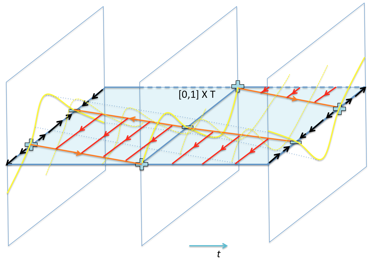
Figure 8. A homotopy 𝒉˘\breve{\bm{{h}}} which translates the initial vector field 𝒉\bm{{h}} by half a S1S^{1}-cycle, showing how the Euler chain is carried along the zero set (orange) of 𝒉˘\breve{\bm{{h}}}. Rotation by a full cycle will return the Euler chain to its original position, with the same homology class.
Refer to caption
Figure 9. A homotopy 𝒉˘\breve{\bm{{h}}} which changes the homology class of an Euler chain. Note that there is no open ball of TT within which the singular set of 𝒉t\bm{{h}}_{t} stays for all t[0,1]t\in[0,1]. Rather, such an “enveloping open set” contains an S1S^{1} cycle.

One shows [26] that the above assignment [l][l][l]\mapsto[l^{\prime}] is independent of the choices of homotopy and of Σ\Sigma, descending to an affine map ϕ𝒉,𝒉:𝔈𝔲𝔩(T,𝒲𝒉)𝔈𝔲𝔩(T,𝒲𝒉)\phi_{\bm{{h}}^{\prime},\bm{{h}}}:\mathfrak{Eul}(T,\mathcal{W}_{\bm{{h}}})\rightarrow\mathfrak{Eul}(T,\mathcal{W}_{\bm{{h}}^{\prime}}). Furthermore, one has the properties ϕ𝒉′′,𝒉=ϕ𝒉′′,𝒉ϕ𝒉,𝒉\phi_{\bm{{h}}^{\prime\prime},\bm{{h}}}=\phi_{\bm{{h}}^{\prime\prime},\bm{{h}}^{\prime}}\circ\phi_{\bm{{h}}^{\prime},\bm{{h}}}, and ϕ𝒉,𝒉=id\phi_{\bm{{h}},\bm{{h}}}=\text{id}, so each 𝔈𝔲𝔩(T,𝒲𝒉)\mathfrak{Eul}(T,\mathcal{W}_{\bm{{h}}}) is canonically isomorphic to a single affine space (which for oriented TT can be taken to be the space of smooth Euler structures 𝔳𝔢𝔠𝔱(T)\mathfrak{vect}(T) in Definition 3.1) over H1(T,)H_{1}(T,{\mathbb{Z}}) [26]. In particular, when a non-singular 𝒉ref\bm{{h}}_{\text{ref}} in 𝔳𝔢𝔠𝔱(T)\mathfrak{vect}(T) has been chosen, a possibly singular 𝒉\bm{{h}} has an associated Euler chain ll.

Example 3.2.

If there is a 𝒉˘\breve{\bm{{h}}} such that the local charges 𝒲t\mathcal{W}_{t} are simply moved around smoothly and disjointly without creation/annihilation, i.e. there is a smooth 1-parameter family of diffeomorphisms φt\varphi_{t} of TT taking 𝒲0\mathcal{W}_{0} to 𝒲t\mathcal{W}_{t}, t[0,1]t\in[0,1], then the zero set W˘\breve{W} of 𝒉˘\breve{\bm{{h}}} is simply a set of disjoint lines representing the trajectories of the local charges. An initial Euler chain ll is “carried along W˘\breve{W}” to the final Euler chain ll^{\prime} (Fig. 8).

Suppose 𝒉,𝒉\bm{{h}},\bm{{h}}^{\prime} have the same 0-chains of local charges, 𝒲=𝒲𝒉=𝒲𝒉\mathcal{W}=\mathcal{W}_{\bm{{h}}}=\mathcal{W}_{\bm{{h}}^{\prime}}. Then the endomorphism ϕ𝒉,𝒉:𝔈𝔲𝔩(T,𝒲)𝔈𝔲𝔩(T,𝒲)\phi_{\bm{{h}}^{\prime},\bm{{h}}}:\mathfrak{Eul}(T,\mathcal{W})\rightarrow\mathfrak{Eul}(T,\mathcal{W}) can be thought of as the homological change in the Euler chains, [l][l][l]\mapsto[l^{\prime}], under a non-degenerate homotopy 𝒉˘\breve{\bm{{h}}} taking 𝒉\bm{{h}} to 𝒉\bm{{h}}^{\prime}. Specifically, ll=𝒲˘Pl^{\prime}-l=\breve{\mathcal{W}}-\partial P can be pushed forward under the projection pp to a 1-chain on TT, also written lll^{\prime}-l, which is actually a cycle. Then [l][l]H1(T,)[l^{\prime}]-[l]\in H_{1}(T,{\mathbb{Z}}) is a “homological difference” between 𝒉\bm{{h}} and 𝒉\bm{{h}}^{\prime}; this difference was called a Chern–Simons class cs(𝒉,𝒉)\text{cs}(\bm{{h}},\bm{{h}}^{\prime}) in [12, 44]. For 𝒉,𝒉\bm{{h}},\bm{{h^{\prime}}} having different local charges, cs(𝒉,𝒉)\text{cs}(\bm{{h}},\bm{{h}}^{\prime}) is defined similarly, as a 1-chain modulo boundaries .

Example 3.3.

Suppose further that there is a non-degenerate homotopy 𝒉˘\breve{\bm{{h}}} which stays non-singular outside some open ball in TT (necessarily containing W𝒉=W𝒉W_{\bm{{h}}}=W_{\bm{{h}}^{\prime}}). Then an initial Euler chain ll does not pick up any nonzero element of H1(T,)H_{1}(T,{\mathbb{Z}}), so [l]=[l][l^{\prime}]=[l] (Fig. 7, 9).

3.4. Euler chain representation of a semimetal

The upshot of introducing Euler chains is that we can use them to represent globally the topological data of a semimetal band structure, whenever vector fields are used to parameterise semimetal Hamiltonians. This is certainly the case for 2×22\times 2 Hamiltonians in 3D, and more generally for Dirac-type Hamiltonians in higher dimensions. The singular points W𝒉W_{\bm{{h}}} of 𝒉\bm{{h}} are the band crossings of HH, and the local charge information is contained in the 0-chain 𝒲𝒉\mathcal{W}_{\bm{{h}}}. Each 𝒉\bm{{h}} can be associated with an Euler chain class in H1(T,W𝒉,)H_{1}(T,W_{\bm{{h}}},{\mathbb{Z}}) by the prescription of the previous subsection, and vector fields with the same local charges but homologically different Euler chains cannot he homotoped whilst keeping the singular set within an open ball (in particular, while keeping the singular set fixed). When we generalise to Kervaire chains for bilinear Hamiltonians later, it will be convenient to use an alternative prescription to associate an Euler (or Kervaire) chain to a semimetal Hamiltonian.

This alternative prescription uses a definition of Euler structures which follows that given in Section 3.2.1, but which is defined in terms of singular vector fields. Let 𝒮\mathcal{S} be the sphere bundle of the tangent bundle of TT, and 𝒮|TW,𝒮|DW=Sd1×DW,𝒮|SW=Sd1×SW\mathcal{S}|_{T\setminus W},\mathcal{S}|_{D_{W}}=S^{d-1}\times D_{W},\mathcal{S}|_{S_{W}}=S^{d-1}\times S_{W} be the restrictions of 𝒮\mathcal{S} to the subspaces of TT appearing in our MV-sequence, and let pp denote the various bundle projections. All these sphere bundles have vanishing Euler class. There is also an MV-sequence for the cover {𝒮|TW,𝒮|DW}\{\mathcal{S}|_{T\setminus W},\mathcal{S}|_{D_{W}}\} of 𝒮\mathcal{S}, which has intersection 𝒮|SW\mathcal{S}|_{S_{W}}, and we write Σ~\widetilde{\Sigma} for its connecting maps. Let 𝒉ref\bm{{h}}_{\text{ref}} be a non-singular vector field on TT, then 𝒉^refp=id\hat{\bm{{h}}}_{\text{ref}}^{*}\circ p^{*}=\text{id}.

Consider the semimetal MV-sequence and its dual homology sequence, where we have suppressed the integer coefficients,

    0          Hd1(T)    PD          ι         Hd1(TW)    PD          β         Hd1(SW)    PD          Σ         Hd(T)    PD                0   0          H1(T)          H1(T,W)             H0(W)    Σ         H0(T)          0    .\lx@xy@svg{\hbox{\raise 2.5pt\hbox{\kern 5.5pt\hbox{\ignorespaces\ignorespaces\ignorespaces\hbox{\vtop{\halign{\entry@#!@&&\entry@@#!@\cr&&&&&\cr&&&&&\crcr}}}\ignorespaces{\hbox{\kern-5.5pt\raise 0.0pt\hbox{\hbox{\kern 0.0pt\raise 0.0pt\hbox{\hbox{\kern 3.0pt\raise-2.5pt\hbox{$\textstyle{0\ignorespaces\ignorespaces\ignorespaces\ignorespaces}$}}}}}}}\ignorespaces\ignorespaces\ignorespaces\ignorespaces{}{\hbox{\lx@xy@droprule}}\ignorespaces{\hbox{\kern 29.5pt\raise 0.0pt\hbox{\hbox{\kern 0.0pt\raise 0.0pt\hbox{\lx@xy@tip{1}\lx@xy@tip{-1}}}}}}{\hbox{\lx@xy@droprule}}{\hbox{\lx@xy@droprule}}{\hbox{\kern 29.5pt\raise 0.0pt\hbox{\hbox{\kern 0.0pt\raise 0.0pt\hbox{\hbox{\kern 3.0pt\raise-2.5pt\hbox{$\textstyle{H^{d-1}(T)\ignorespaces\ignorespaces\ignorespaces\ignorespaces\ignorespaces\ignorespaces\ignorespaces\ignorespaces}$}}}}}}}\ignorespaces\ignorespaces\ignorespaces\ignorespaces{}{\hbox{\lx@xy@droprule}}\ignorespaces\ignorespaces\ignorespaces{\hbox{\kern 32.84357pt\raise-16.2475pt\hbox{{}\hbox{\kern 0.0pt\raise 0.0pt\hbox{\hbox{\kern 3.0pt\hbox{\hbox{\kern 0.0pt\raise-2.39168pt\hbox{$\scriptstyle{\text{PD}}$}}}\kern 3.0pt}}}}}}\ignorespaces{\hbox{\kern 50.23944pt\raise-24.49501pt\hbox{\hbox{\kern 0.0pt\raise 0.0pt\hbox{\lx@xy@tip{1}\lx@xy@tip{-1}}}}}}{\hbox{\lx@xy@droprule}}{\hbox{\lx@xy@droprule}}\ignorespaces\ignorespaces\ignorespaces\ignorespaces{}{\hbox{\lx@xy@droprule}}\ignorespaces\ignorespaces\ignorespaces{\hbox{\kern 82.1727pt\raise 5.67209pt\hbox{{}\hbox{\kern 0.0pt\raise 0.0pt\hbox{\hbox{\kern 3.0pt\hbox{\hbox{\kern 0.0pt\raise-2.67209pt\hbox{$\scriptstyle{\iota^{*}}$}}}\kern 3.0pt}}}}}}\ignorespaces{\hbox{\kern 94.97888pt\raise 0.0pt\hbox{\hbox{\kern 0.0pt\raise 0.0pt\hbox{\lx@xy@tip{1}\lx@xy@tip{-1}}}}}}{\hbox{\lx@xy@droprule}}{\hbox{\lx@xy@droprule}}{\hbox{\kern 94.97888pt\raise 0.0pt\hbox{\hbox{\kern 0.0pt\raise 0.0pt\hbox{\hbox{\kern 3.0pt\raise-2.5pt\hbox{$\textstyle{H^{d-1}(T\setminus W)\ignorespaces\ignorespaces\ignorespaces\ignorespaces\ignorespaces\ignorespaces\ignorespaces\ignorespaces}$}}}}}}}\ignorespaces\ignorespaces\ignorespaces\ignorespaces{}{\hbox{\lx@xy@droprule}}\ignorespaces\ignorespaces\ignorespaces{\hbox{\kern 109.85019pt\raise-16.2475pt\hbox{{}\hbox{\kern 0.0pt\raise 0.0pt\hbox{\hbox{\kern 3.0pt\hbox{\hbox{\kern 0.0pt\raise-2.39168pt\hbox{$\scriptstyle{\text{PD}}$}}}\kern 3.0pt}}}}}}\ignorespaces{\hbox{\kern 127.24606pt\raise-24.49501pt\hbox{\hbox{\kern 0.0pt\raise 0.0pt\hbox{\lx@xy@tip{1}\lx@xy@tip{-1}}}}}}{\hbox{\lx@xy@droprule}}{\hbox{\lx@xy@droprule}}\ignorespaces\ignorespaces\ignorespaces\ignorespaces{}{\hbox{\lx@xy@droprule}}\ignorespaces\ignorespaces\ignorespaces{\hbox{\kern 162.6254pt\raise 6.1111pt\hbox{{}\hbox{\kern 0.0pt\raise 0.0pt\hbox{\hbox{\kern 3.0pt\hbox{\hbox{\kern 0.0pt\raise-1.75pt\hbox{$\scriptstyle{\beta}$}}}\kern 3.0pt}}}}}}\ignorespaces{\hbox{\kern 183.51324pt\raise 0.0pt\hbox{\hbox{\kern 0.0pt\raise 0.0pt\hbox{\lx@xy@tip{1}\lx@xy@tip{-1}}}}}}{\hbox{\lx@xy@droprule}}{\hbox{\lx@xy@droprule}}{\hbox{\kern 183.51324pt\raise 0.0pt\hbox{\hbox{\kern 0.0pt\raise 0.0pt\hbox{\hbox{\kern 3.0pt\raise-2.5pt\hbox{$\textstyle{H^{d-1}(S_{W})\ignorespaces\ignorespaces\ignorespaces\ignorespaces\ignorespaces\ignorespaces\ignorespaces\ignorespaces}$}}}}}}}\ignorespaces\ignorespaces\ignorespaces\ignorespaces{}{\hbox{\lx@xy@droprule}}\ignorespaces\ignorespaces\ignorespaces{\hbox{\kern 191.14326pt\raise-16.2475pt\hbox{{}\hbox{\kern 0.0pt\raise 0.0pt\hbox{\hbox{\kern 3.0pt\hbox{\hbox{\kern 0.0pt\raise-2.39168pt\hbox{$\scriptstyle{\text{PD}}$}}}\kern 3.0pt}}}}}}\ignorespaces{\hbox{\kern 208.53914pt\raise-24.49501pt\hbox{\hbox{\kern 0.0pt\raise 0.0pt\hbox{\lx@xy@tip{1}\lx@xy@tip{-1}}}}}}{\hbox{\lx@xy@droprule}}{\hbox{\lx@xy@droprule}}\ignorespaces\ignorespaces\ignorespaces\ignorespaces{}{\hbox{\lx@xy@droprule}}\ignorespaces\ignorespaces\ignorespaces{\hbox{\kern 235.89748pt\raise 5.39168pt\hbox{{}\hbox{\kern 0.0pt\raise 0.0pt\hbox{\hbox{\kern 3.0pt\hbox{\hbox{\kern 0.0pt\raise-2.39168pt\hbox{$\scriptstyle{\Sigma}$}}}\kern 3.0pt}}}}}}\ignorespaces{\hbox{\kern 257.56503pt\raise 0.0pt\hbox{\hbox{\kern 0.0pt\raise 0.0pt\hbox{\lx@xy@tip{1}\lx@xy@tip{-1}}}}}}{\hbox{\lx@xy@droprule}}{\hbox{\lx@xy@droprule}}{\hbox{\kern 257.56503pt\raise 0.0pt\hbox{\hbox{\kern 0.0pt\raise 0.0pt\hbox{\hbox{\kern 3.0pt\raise-2.5pt\hbox{$\textstyle{H^{d}(T)\ignorespaces\ignorespaces\ignorespaces\ignorespaces\ignorespaces\ignorespaces\ignorespaces\ignorespaces}$}}}}}}}\ignorespaces\ignorespaces\ignorespaces\ignorespaces{}{\hbox{\lx@xy@droprule}}\ignorespaces\ignorespaces\ignorespaces{\hbox{\kern 257.5683pt\raise-16.2475pt\hbox{{}\hbox{\kern 0.0pt\raise 0.0pt\hbox{\hbox{\kern 3.0pt\hbox{\hbox{\kern 0.0pt\raise-2.39168pt\hbox{$\scriptstyle{\text{PD}}$}}}\kern 3.0pt}}}}}}\ignorespaces{\hbox{\kern 274.96417pt\raise-24.49501pt\hbox{\hbox{\kern 0.0pt\raise 0.0pt\hbox{\lx@xy@tip{1}\lx@xy@tip{-1}}}}}}{\hbox{\lx@xy@droprule}}{\hbox{\lx@xy@droprule}}\ignorespaces\ignorespaces\ignorespaces\ignorespaces{}{\hbox{\lx@xy@droprule}}\ignorespaces{\hbox{\kern 316.36331pt\raise 0.0pt\hbox{\hbox{\kern 0.0pt\raise 0.0pt\hbox{\lx@xy@tip{1}\lx@xy@tip{-1}}}}}}{\hbox{\lx@xy@droprule}}{\hbox{\lx@xy@droprule}}{\hbox{\kern 316.36331pt\raise 0.0pt\hbox{\hbox{\kern 0.0pt\raise 0.0pt\hbox{\hbox{\kern 3.0pt\raise-2.5pt\hbox{$\textstyle{0}$}}}}}}}{\hbox{\kern-5.5pt\raise-32.49501pt\hbox{\hbox{\kern 0.0pt\raise 0.0pt\hbox{\hbox{\kern 3.0pt\raise-2.5pt\hbox{$\textstyle{0\ignorespaces\ignorespaces\ignorespaces\ignorespaces}$}}}}}}}\ignorespaces\ignorespaces\ignorespaces\ignorespaces{}{\hbox{\lx@xy@droprule}}\ignorespaces{\hbox{\kern 32.92867pt\raise-32.49501pt\hbox{\hbox{\kern 0.0pt\raise 0.0pt\hbox{\lx@xy@tip{1}\lx@xy@tip{-1}}}}}}{\hbox{\lx@xy@droprule}}{\hbox{\lx@xy@droprule}}{\hbox{\kern 32.92867pt\raise-32.49501pt\hbox{\hbox{\kern 0.0pt\raise 0.0pt\hbox{\hbox{\kern 3.0pt\raise-2.5pt\hbox{$\textstyle{H_{1}(T)\ignorespaces\ignorespaces\ignorespaces\ignorespaces}$}}}}}}}\ignorespaces\ignorespaces\ignorespaces\ignorespaces{}{\hbox{\lx@xy@droprule}}\ignorespaces{\hbox{\kern 102.57419pt\raise-32.49501pt\hbox{\hbox{\kern 0.0pt\raise 0.0pt\hbox{\lx@xy@tip{1}\lx@xy@tip{-1}}}}}}{\hbox{\lx@xy@droprule}}{\hbox{\lx@xy@droprule}}{\hbox{\kern 102.57419pt\raise-32.49501pt\hbox{\hbox{\kern 0.0pt\raise 0.0pt\hbox{\hbox{\kern 3.0pt\raise-2.5pt\hbox{$\textstyle{H_{1}(T,W)\ignorespaces\ignorespaces\ignorespaces\ignorespaces}$}}}}}}}\ignorespaces\ignorespaces\ignorespaces\ignorespaces{}{\hbox{\lx@xy@droprule}}\ignorespaces\ignorespaces\ignorespaces{\hbox{\kern 162.75735pt\raise-27.06445pt\hbox{{}\hbox{\kern 0.0pt\raise 0.0pt\hbox{\hbox{\kern 3.0pt\hbox{\hbox{\kern 0.0pt\raise-2.43056pt\hbox{$\scriptstyle{\partial}$}}}\kern 3.0pt}}}}}}\ignorespaces{\hbox{\kern 189.42802pt\raise-32.49501pt\hbox{\hbox{\kern 0.0pt\raise 0.0pt\hbox{\lx@xy@tip{1}\lx@xy@tip{-1}}}}}}{\hbox{\lx@xy@droprule}}{\hbox{\lx@xy@droprule}}{\hbox{\kern 189.42802pt\raise-32.49501pt\hbox{\hbox{\kern 0.0pt\raise 0.0pt\hbox{\hbox{\kern 3.0pt\raise-2.5pt\hbox{$\textstyle{H_{0}(W)\ignorespaces\ignorespaces\ignorespaces\ignorespaces}$}}}}}}}\ignorespaces\ignorespaces\ignorespaces\ignorespaces{}{\hbox{\lx@xy@droprule}}\ignorespaces\ignorespaces\ignorespaces{\hbox{\kern 235.89748pt\raise-27.10333pt\hbox{{}\hbox{\kern 0.0pt\raise 0.0pt\hbox{\hbox{\kern 3.0pt\hbox{\hbox{\kern 0.0pt\raise-2.39168pt\hbox{$\scriptstyle{\Sigma}$}}}\kern 3.0pt}}}}}}\ignorespaces{\hbox{\kern 257.6534pt\raise-32.49501pt\hbox{\hbox{\kern 0.0pt\raise 0.0pt\hbox{\lx@xy@tip{1}\lx@xy@tip{-1}}}}}}{\hbox{\lx@xy@droprule}}{\hbox{\lx@xy@droprule}}{\hbox{\kern 257.6534pt\raise-32.49501pt\hbox{\hbox{\kern 0.0pt\raise 0.0pt\hbox{\hbox{\kern 3.0pt\raise-2.5pt\hbox{$\textstyle{H_{0}(T)\ignorespaces\ignorespaces\ignorespaces\ignorespaces}$}}}}}}}\ignorespaces\ignorespaces\ignorespaces\ignorespaces{}{\hbox{\lx@xy@droprule}}\ignorespaces{\hbox{\kern 316.36331pt\raise-32.49501pt\hbox{\hbox{\kern 0.0pt\raise 0.0pt\hbox{\lx@xy@tip{1}\lx@xy@tip{-1}}}}}}{\hbox{\lx@xy@droprule}}{\hbox{\lx@xy@droprule}}{\hbox{\kern 316.36331pt\raise-32.49501pt\hbox{\hbox{\kern 0.0pt\raise 0.0pt\hbox{\hbox{\kern 3.0pt\raise-2.5pt\hbox{$\textstyle{0}$}}}}}}}\ignorespaces}}}}\ignorespaces.

The local charges can be thought of as a 0-chain 𝒲\mathcal{W} on WTW\subset T, or dually as an element PD(𝒲)\text{PD}(\mathcal{W}) in Hd1(SW)H^{d-1}(S_{W}); in either case they are required to have total charge zero.

Definition 3.4.

For a 0-chain 𝒲\mathcal{W} of local charges on TT, with total charge 0 and defined on WTW\subset T, we write 𝔠𝔬𝔈𝔲𝔩(T,𝒲)\mathfrak{coEul}(T,\mathcal{W}) for the image of 𝔈𝔲𝔩(T,𝒲)\mathfrak{Eul}(T,\mathcal{W}) in Hd1(TW)H^{d-1}(T\setminus W) under Poincaré duality; equivalently this is the inverse image of PD(𝒲)\text{PD}(\mathcal{W}) under β\beta.

We combine the cohomology Mayer–Vietoris (horizontal) and Gysin sequences (vertical) for TT and 𝒮\mathcal{S},

(3.2)     0          0          0          0          Hd1(T)    p          ι         Hd1(TW)    p          β         Hd1(SW)    p          Σ            0          Hd1(𝒮)           p         Hd1(𝒮|TW)Hd1(𝒮|DW)           p         Hd1(𝒮|SW)    Σ~          p            0          H0(T)                 H0(TW)H0(DW)                 H0(SW)                    0   0   0    ,\lx@xy@svg{\hbox{\raise 2.5pt\hbox{\kern 5.5pt\hbox{\ignorespaces\ignorespaces\ignorespaces\hbox{\vtop{\halign{\entry@#!@&&\entry@@#!@\cr&&&&\cr&&&&\cr&&&&\cr&&&&\cr&&&&\crcr}}}\ignorespaces{\hbox{\kern-3.0pt\raise 0.0pt\hbox{\hbox{\kern 0.0pt\raise 0.0pt\hbox{\hbox{\kern 3.0pt\raise-2.5pt\hbox{$\textstyle{}$}}}}}}}{\hbox{\kern 44.73944pt\raise 0.0pt\hbox{\hbox{\kern 0.0pt\raise 0.0pt\hbox{\hbox{\kern 3.0pt\raise-2.5pt\hbox{$\textstyle{0\ignorespaces\ignorespaces\ignorespaces\ignorespaces}$}}}}}}}\ignorespaces\ignorespaces\ignorespaces\ignorespaces{}{\hbox{\lx@xy@droprule}}\ignorespaces{\hbox{\kern 50.23944pt\raise-22.9772pt\hbox{\hbox{\kern 0.0pt\raise 0.0pt\hbox{\lx@xy@tip{1}\lx@xy@tip{-1}}}}}}{\hbox{\lx@xy@droprule}}{\hbox{\lx@xy@droprule}}{\hbox{\kern 153.25188pt\raise 0.0pt\hbox{\hbox{\kern 0.0pt\raise 0.0pt\hbox{\hbox{\kern 3.0pt\raise-2.5pt\hbox{$\textstyle{0\ignorespaces\ignorespaces\ignorespaces\ignorespaces}$}}}}}}}\ignorespaces\ignorespaces\ignorespaces\ignorespaces{}{\hbox{\lx@xy@droprule}}\ignorespaces{\hbox{\kern 158.75188pt\raise-22.9772pt\hbox{\hbox{\kern 0.0pt\raise 0.0pt\hbox{\lx@xy@tip{1}\lx@xy@tip{-1}}}}}}{\hbox{\lx@xy@droprule}}{\hbox{\lx@xy@droprule}}{\hbox{\kern 269.0932pt\raise 0.0pt\hbox{\hbox{\kern 0.0pt\raise 0.0pt\hbox{\hbox{\kern 3.0pt\raise-2.5pt\hbox{$\textstyle{0\ignorespaces\ignorespaces\ignorespaces\ignorespaces}$}}}}}}}\ignorespaces\ignorespaces\ignorespaces\ignorespaces{}{\hbox{\lx@xy@droprule}}\ignorespaces{\hbox{\kern 274.5932pt\raise-22.9772pt\hbox{\hbox{\kern 0.0pt\raise 0.0pt\hbox{\lx@xy@tip{1}\lx@xy@tip{-1}}}}}}{\hbox{\lx@xy@droprule}}{\hbox{\lx@xy@droprule}}{\hbox{\kern 330.41153pt\raise 0.0pt\hbox{\hbox{\kern 0.0pt\raise 0.0pt\hbox{\hbox{\kern 3.0pt\raise-2.5pt\hbox{$\textstyle{}$}}}}}}}{\hbox{\kern-5.5pt\raise-31.96722pt\hbox{\hbox{\kern 0.0pt\raise 0.0pt\hbox{\hbox{\kern 3.0pt\raise-2.5pt\hbox{$\textstyle{0\ignorespaces\ignorespaces\ignorespaces\ignorespaces}$}}}}}}}\ignorespaces\ignorespaces\ignorespaces\ignorespaces{}{\hbox{\lx@xy@droprule}}\ignorespaces{\hbox{\kern 29.5pt\raise-31.96722pt\hbox{\hbox{\kern 0.0pt\raise 0.0pt\hbox{\lx@xy@tip{1}\lx@xy@tip{-1}}}}}}{\hbox{\lx@xy@droprule}}{\hbox{\lx@xy@droprule}}{\hbox{\kern 29.5pt\raise-31.96722pt\hbox{\hbox{\kern 0.0pt\raise 0.0pt\hbox{\hbox{\kern 3.0pt\raise-2.5pt\hbox{$\textstyle{H^{d-1}(T)\ignorespaces\ignorespaces\ignorespaces\ignorespaces\ignorespaces\ignorespaces\ignorespaces\ignorespaces}$}}}}}}}\ignorespaces\ignorespaces\ignorespaces\ignorespaces{}{\hbox{\lx@xy@droprule}}\ignorespaces\ignorespaces\ignorespaces{\hbox{\kern 35.93651pt\raise-48.46223pt\hbox{{}\hbox{\kern 0.0pt\raise 0.0pt\hbox{\hbox{\kern 3.0pt\hbox{\hbox{\kern 0.0pt\raise-1.99155pt\hbox{$\scriptstyle{p^{*}}$}}}\kern 3.0pt}}}}}}\ignorespaces{\hbox{\kern 50.23944pt\raise-55.96722pt\hbox{\hbox{\kern 0.0pt\raise 0.0pt\hbox{\lx@xy@tip{1}\lx@xy@tip{-1}}}}}}{\hbox{\lx@xy@droprule}}{\hbox{\lx@xy@droprule}}\ignorespaces\ignorespaces\ignorespaces\ignorespaces{}{\hbox{\lx@xy@droprule}}\ignorespaces\ignorespaces\ignorespaces{\hbox{\kern 97.9256pt\raise-26.29514pt\hbox{{}\hbox{\kern 0.0pt\raise 0.0pt\hbox{\hbox{\kern 3.0pt\hbox{\hbox{\kern 0.0pt\raise-2.67209pt\hbox{$\scriptstyle{\iota^{*}}$}}}\kern 3.0pt}}}}}}\ignorespaces{\hbox{\kern 126.4847pt\raise-31.96722pt\hbox{\hbox{\kern 0.0pt\raise 0.0pt\hbox{\lx@xy@tip{1}\lx@xy@tip{-1}}}}}}{\hbox{\lx@xy@droprule}}{\hbox{\lx@xy@droprule}}{\hbox{\kern 126.4847pt\raise-31.96722pt\hbox{\hbox{\kern 0.0pt\raise 0.0pt\hbox{\hbox{\kern 3.0pt\raise-2.5pt\hbox{$\textstyle{H^{d-1}(T\setminus W)\ignorespaces\ignorespaces\ignorespaces\ignorespaces\ignorespaces\ignorespaces\ignorespaces\ignorespaces}$}}}}}}}\ignorespaces\ignorespaces\ignorespaces\ignorespaces{}{\hbox{\lx@xy@droprule}}\ignorespaces\ignorespaces\ignorespaces{\hbox{\kern 144.44894pt\raise-48.46223pt\hbox{{}\hbox{\kern 0.0pt\raise 0.0pt\hbox{\hbox{\kern 3.0pt\hbox{\hbox{\kern 0.0pt\raise-1.99155pt\hbox{$\scriptstyle{p^{*}}$}}}\kern 3.0pt}}}}}}\ignorespaces{\hbox{\kern 158.75188pt\raise-55.96722pt\hbox{\hbox{\kern 0.0pt\raise 0.0pt\hbox{\lx@xy@tip{1}\lx@xy@tip{-1}}}}}}{\hbox{\lx@xy@droprule}}{\hbox{\lx@xy@droprule}}\ignorespaces\ignorespaces\ignorespaces\ignorespaces{}{\hbox{\lx@xy@droprule}}\ignorespaces\ignorespaces\ignorespaces{\hbox{\kern 211.40533pt\raise-25.85612pt\hbox{{}\hbox{\kern 0.0pt\raise 0.0pt\hbox{\hbox{\kern 3.0pt\hbox{\hbox{\kern 0.0pt\raise-1.75pt\hbox{$\scriptstyle{\beta}$}}}\kern 3.0pt}}}}}}\ignorespaces{\hbox{\kern 249.5673pt\raise-31.96722pt\hbox{\hbox{\kern 0.0pt\raise 0.0pt\hbox{\lx@xy@tip{1}\lx@xy@tip{-1}}}}}}{\hbox{\lx@xy@droprule}}{\hbox{\lx@xy@droprule}}{\hbox{\kern 249.5673pt\raise-31.96722pt\hbox{\hbox{\kern 0.0pt\raise 0.0pt\hbox{\hbox{\kern 3.0pt\raise-2.5pt\hbox{$\textstyle{H^{d-1}(S_{W})\ignorespaces\ignorespaces\ignorespaces\ignorespaces\ignorespaces\ignorespaces\ignorespaces\ignorespaces}$}}}}}}}\ignorespaces\ignorespaces\ignorespaces\ignorespaces{}{\hbox{\lx@xy@droprule}}\ignorespaces\ignorespaces\ignorespaces{\hbox{\kern 260.29027pt\raise-48.46223pt\hbox{{}\hbox{\kern 0.0pt\raise 0.0pt\hbox{\hbox{\kern 3.0pt\hbox{\hbox{\kern 0.0pt\raise-1.99155pt\hbox{$\scriptstyle{p^{*}}$}}}\kern 3.0pt}}}}}}\ignorespaces{\hbox{\kern 274.5932pt\raise-55.96722pt\hbox{\hbox{\kern 0.0pt\raise 0.0pt\hbox{\lx@xy@tip{1}\lx@xy@tip{-1}}}}}}{\hbox{\lx@xy@droprule}}{\hbox{\lx@xy@droprule}}\ignorespaces\ignorespaces\ignorespaces\ignorespaces{}{\hbox{\lx@xy@droprule}}\ignorespaces\ignorespaces\ignorespaces{\hbox{\kern 294.05095pt\raise-26.57555pt\hbox{{}\hbox{\kern 0.0pt\raise 0.0pt\hbox{\hbox{\kern 3.0pt\hbox{\hbox{\kern 0.0pt\raise-2.39168pt\hbox{$\scriptstyle{\hskip 8.19447pt\Sigma}$}}}\kern 3.0pt}}}}}}\ignorespaces{\hbox{\kern 326.66153pt\raise-31.96722pt\hbox{\hbox{\kern 0.0pt\raise 0.0pt\hbox{\lx@xy@tip{1}\lx@xy@tip{-1}}}}}}{\hbox{\lx@xy@droprule}}{\hbox{\lx@xy@droprule}}{\hbox{\kern 326.66153pt\raise-31.96722pt\hbox{\hbox{\kern 0.0pt\raise 0.0pt\hbox{\hbox{\kern 3.0pt\raise-2.5pt\hbox{$\textstyle{\cdots}$}}}}}}}{\hbox{\kern-5.5pt\raise-64.95724pt\hbox{\hbox{\kern 0.0pt\raise 0.0pt\hbox{\hbox{\kern 3.0pt\raise-2.5pt\hbox{$\textstyle{0\ignorespaces\ignorespaces\ignorespaces\ignorespaces}$}}}}}}}\ignorespaces\ignorespaces\ignorespaces\ignorespaces{}{\hbox{\lx@xy@droprule}}\ignorespaces{\hbox{\kern 30.33855pt\raise-64.95724pt\hbox{\hbox{\kern 0.0pt\raise 0.0pt\hbox{\lx@xy@tip{1}\lx@xy@tip{-1}}}}}}{\hbox{\lx@xy@droprule}}{\hbox{\lx@xy@droprule}}{\hbox{\kern 30.33855pt\raise-64.95724pt\hbox{\hbox{\kern 0.0pt\raise 0.0pt\hbox{\hbox{\kern 3.0pt\raise-2.5pt\hbox{$\textstyle{H^{d-1}(\mathcal{S})\ignorespaces\ignorespaces\ignorespaces\ignorespaces\ignorespaces\ignorespaces\ignorespaces\ignorespaces}$}}}}}}}\ignorespaces\ignorespaces\ignorespaces\ignorespaces{}{\hbox{\lx@xy@droprule}}\ignorespaces{\hbox{\kern 94.97888pt\raise-64.95724pt\hbox{\hbox{\kern 0.0pt\raise 0.0pt\hbox{\lx@xy@tip{1}\lx@xy@tip{-1}}}}}}{\hbox{\lx@xy@droprule}}{\hbox{\lx@xy@droprule}}\ignorespaces\ignorespaces\ignorespaces\ignorespaces{}{\hbox{\lx@xy@droprule}}\ignorespaces\ignorespaces\ignorespaces{\hbox{\kern 35.93651pt\raise-81.36475pt\hbox{{}\hbox{\kern 0.0pt\raise 0.0pt\hbox{\hbox{\kern 3.0pt\hbox{\hbox{\kern 0.0pt\raise-0.8264pt\hbox{$\scriptstyle{p_{*}}$}}}\kern 3.0pt}}}}}}\ignorespaces{\hbox{\kern 50.23944pt\raise-89.13223pt\hbox{\hbox{\kern 0.0pt\raise 0.0pt\hbox{\lx@xy@tip{1}\lx@xy@tip{-1}}}}}}{\hbox{\lx@xy@droprule}}{\hbox{\lx@xy@droprule}}{\hbox{\kern 94.97888pt\raise-64.95724pt\hbox{\hbox{\kern 0.0pt\raise 0.0pt\hbox{\hbox{\kern 3.0pt\raise-2.5pt\hbox{$\textstyle{H^{d-1}(\mathcal{S}|_{T\setminus W})\oplus H^{d-1}(\mathcal{S}|_{D_{W}})\ignorespaces\ignorespaces\ignorespaces\ignorespaces\ignorespaces\ignorespaces\ignorespaces\ignorespaces}$}}}}}}}\ignorespaces\ignorespaces\ignorespaces\ignorespaces{}{\hbox{\lx@xy@droprule}}\ignorespaces{\hbox{\kern 246.52487pt\raise-64.95724pt\hbox{\hbox{\kern 0.0pt\raise 0.0pt\hbox{\lx@xy@tip{1}\lx@xy@tip{-1}}}}}}{\hbox{\lx@xy@droprule}}{\hbox{\lx@xy@droprule}}\ignorespaces\ignorespaces\ignorespaces\ignorespaces{}{\hbox{\lx@xy@droprule}}\ignorespaces\ignorespaces\ignorespaces{\hbox{\kern 144.44894pt\raise-81.36475pt\hbox{{}\hbox{\kern 0.0pt\raise 0.0pt\hbox{\hbox{\kern 3.0pt\hbox{\hbox{\kern 0.0pt\raise-0.8264pt\hbox{$\scriptstyle{p_{*}}$}}}\kern 3.0pt}}}}}}\ignorespaces{\hbox{\kern 158.75188pt\raise-89.13223pt\hbox{\hbox{\kern 0.0pt\raise 0.0pt\hbox{\lx@xy@tip{1}\lx@xy@tip{-1}}}}}}{\hbox{\lx@xy@droprule}}{\hbox{\lx@xy@droprule}}{\hbox{\kern 246.52487pt\raise-64.95724pt\hbox{\hbox{\kern 0.0pt\raise 0.0pt\hbox{\hbox{\kern 3.0pt\raise-2.5pt\hbox{$\textstyle{H^{d-1}(\mathcal{S}|_{S_{W}})\ignorespaces\ignorespaces\ignorespaces\ignorespaces\ignorespaces\ignorespaces\ignorespaces\ignorespaces}$}}}}}}}\ignorespaces\ignorespaces\ignorespaces\ignorespaces{}{\hbox{\lx@xy@droprule}}\ignorespaces\ignorespaces\ignorespaces{\hbox{\kern 294.12735pt\raise-58.34613pt\hbox{{}\hbox{\kern 0.0pt\raise 0.0pt\hbox{\hbox{\kern 3.0pt\hbox{\hbox{\kern 0.0pt\raise-3.61111pt\hbox{$\scriptstyle{\hskip 8.19447pt\widetilde{\Sigma}}$}}}\kern 3.0pt}}}}}}\ignorespaces{\hbox{\kern 326.66153pt\raise-64.95724pt\hbox{\hbox{\kern 0.0pt\raise 0.0pt\hbox{\lx@xy@tip{1}\lx@xy@tip{-1}}}}}}{\hbox{\lx@xy@droprule}}{\hbox{\lx@xy@droprule}}\ignorespaces\ignorespaces\ignorespaces\ignorespaces{}{\hbox{\lx@xy@droprule}}\ignorespaces\ignorespaces\ignorespaces{\hbox{\kern 260.29027pt\raise-81.36475pt\hbox{{}\hbox{\kern 0.0pt\raise 0.0pt\hbox{\hbox{\kern 3.0pt\hbox{\hbox{\kern 0.0pt\raise-0.8264pt\hbox{$\scriptstyle{p_{*}}$}}}\kern 3.0pt}}}}}}\ignorespaces{\hbox{\kern 274.5932pt\raise-89.13223pt\hbox{\hbox{\kern 0.0pt\raise 0.0pt\hbox{\lx@xy@tip{1}\lx@xy@tip{-1}}}}}}{\hbox{\lx@xy@droprule}}{\hbox{\lx@xy@droprule}}{\hbox{\kern 326.66153pt\raise-64.95724pt\hbox{\hbox{\kern 0.0pt\raise 0.0pt\hbox{\hbox{\kern 3.0pt\raise-2.5pt\hbox{$\textstyle{\cdots}$}}}}}}}{\hbox{\kern-5.5pt\raise-97.77226pt\hbox{\hbox{\kern 0.0pt\raise 0.0pt\hbox{\hbox{\kern 3.0pt\raise-2.5pt\hbox{$\textstyle{0\ignorespaces\ignorespaces\ignorespaces\ignorespaces}$}}}}}}}\ignorespaces\ignorespaces\ignorespaces\ignorespaces{}{\hbox{\lx@xy@droprule}}\ignorespaces{\hbox{\kern 32.92867pt\raise-97.77226pt\hbox{\hbox{\kern 0.0pt\raise 0.0pt\hbox{\lx@xy@tip{1}\lx@xy@tip{-1}}}}}}{\hbox{\lx@xy@droprule}}{\hbox{\lx@xy@droprule}}{\hbox{\kern 32.92867pt\raise-97.77226pt\hbox{\hbox{\kern 0.0pt\raise 0.0pt\hbox{\hbox{\kern 3.0pt\raise-2.5pt\hbox{$\textstyle{H^{0}(T)\ignorespaces\ignorespaces\ignorespaces\ignorespaces\ignorespaces\ignorespaces\ignorespaces\ignorespaces}$}}}}}}}\ignorespaces\ignorespaces\ignorespaces\ignorespaces{}{\hbox{\lx@xy@droprule}}\ignorespaces{\hbox{\kern 104.28075pt\raise-97.77226pt\hbox{\hbox{\kern 0.0pt\raise 0.0pt\hbox{\lx@xy@tip{1}\lx@xy@tip{-1}}}}}}{\hbox{\lx@xy@droprule}}{\hbox{\lx@xy@droprule}}\ignorespaces\ignorespaces\ignorespaces\ignorespaces{}{\hbox{\lx@xy@droprule}}\ignorespaces{\hbox{\kern 50.23944pt\raise-122.62004pt\hbox{\hbox{\kern 0.0pt\raise 0.0pt\hbox{\lx@xy@tip{1}\lx@xy@tip{-1}}}}}}{\hbox{\lx@xy@droprule}}{\hbox{\lx@xy@droprule}}{\hbox{\kern 104.28075pt\raise-97.77226pt\hbox{\hbox{\kern 0.0pt\raise 0.0pt\hbox{\hbox{\kern 3.0pt\raise-2.5pt\hbox{$\textstyle{H^{0}(T\setminus W)\oplus H^{0}(D_{W})\ignorespaces\ignorespaces\ignorespaces\ignorespaces\ignorespaces\ignorespaces\ignorespaces\ignorespaces}$}}}}}}}\ignorespaces\ignorespaces\ignorespaces\ignorespaces{}{\hbox{\lx@xy@droprule}}\ignorespaces{\hbox{\kern 252.99597pt\raise-97.77226pt\hbox{\hbox{\kern 0.0pt\raise 0.0pt\hbox{\lx@xy@tip{1}\lx@xy@tip{-1}}}}}}{\hbox{\lx@xy@droprule}}{\hbox{\lx@xy@droprule}}\ignorespaces\ignorespaces\ignorespaces\ignorespaces{}{\hbox{\lx@xy@droprule}}\ignorespaces{\hbox{\kern 158.75188pt\raise-122.62004pt\hbox{\hbox{\kern 0.0pt\raise 0.0pt\hbox{\lx@xy@tip{1}\lx@xy@tip{-1}}}}}}{\hbox{\lx@xy@droprule}}{\hbox{\lx@xy@droprule}}{\hbox{\kern 252.99597pt\raise-97.77226pt\hbox{\hbox{\kern 0.0pt\raise 0.0pt\hbox{\hbox{\kern 3.0pt\raise-2.5pt\hbox{$\textstyle{H^{0}(S_{W})\ignorespaces\ignorespaces\ignorespaces\ignorespaces\ignorespaces\ignorespaces\ignorespaces\ignorespaces}$}}}}}}}\ignorespaces\ignorespaces\ignorespaces\ignorespaces{}{\hbox{\lx@xy@droprule}}\ignorespaces{\hbox{\kern 326.66153pt\raise-97.77226pt\hbox{\hbox{\kern 0.0pt\raise 0.0pt\hbox{\lx@xy@tip{1}\lx@xy@tip{-1}}}}}}{\hbox{\lx@xy@droprule}}{\hbox{\lx@xy@droprule}}\ignorespaces\ignorespaces\ignorespaces\ignorespaces{}{\hbox{\lx@xy@droprule}}\ignorespaces{\hbox{\kern 274.5932pt\raise-122.62004pt\hbox{\hbox{\kern 0.0pt\raise 0.0pt\hbox{\lx@xy@tip{1}\lx@xy@tip{-1}}}}}}{\hbox{\lx@xy@droprule}}{\hbox{\lx@xy@droprule}}{\hbox{\kern 326.66153pt\raise-97.77226pt\hbox{\hbox{\kern 0.0pt\raise 0.0pt\hbox{\hbox{\kern 3.0pt\raise-2.5pt\hbox{$\textstyle{\cdots}$}}}}}}}{\hbox{\kern-3.0pt\raise-129.56448pt\hbox{\hbox{\kern 0.0pt\raise 0.0pt\hbox{\hbox{\kern 3.0pt\raise-2.5pt\hbox{$\textstyle{}$}}}}}}}{\hbox{\kern 44.73944pt\raise-129.56448pt\hbox{\hbox{\kern 0.0pt\raise 0.0pt\hbox{\hbox{\kern 3.0pt\raise-2.5pt\hbox{$\textstyle{0}$}}}}}}}{\hbox{\kern 153.25188pt\raise-129.56448pt\hbox{\hbox{\kern 0.0pt\raise 0.0pt\hbox{\hbox{\kern 3.0pt\raise-2.5pt\hbox{$\textstyle{0}$}}}}}}}{\hbox{\kern 269.0932pt\raise-129.56448pt\hbox{\hbox{\kern 0.0pt\raise 0.0pt\hbox{\hbox{\kern 3.0pt\raise-2.5pt\hbox{$\textstyle{0}$}}}}}}}{\hbox{\kern 330.41153pt\raise-129.56448pt\hbox{\hbox{\kern 0.0pt\raise 0.0pt\hbox{\hbox{\kern 3.0pt\raise-2.5pt\hbox{$\textstyle{}$}}}}}}}\ignorespaces}}}}\ignorespaces,

where we have augmented the middle Gysin sequence by a Hd1(𝒮|DW)pH0(DW)H^{d-1}(\mathcal{S}|_{D_{W}})\xrightarrow{p_{*}}H^{0}(D_{W}) piece needed to make the bottom two horizontal MV sequences exact. The horizontal maps are restriction maps (or differences of) and so it is easy to see that the diagram commutes. The middle MV-sequence is, by the Künneth theorem,

0Hd1(𝒮)Hd1(𝒮|TW)Hd1(𝒮|DW)Hd1(SW)H0(SW)Σ~=Σ~1Σ~20\rightarrow H^{d-1}(\mathcal{S})\rightarrow H^{d-1}(\mathcal{S}|_{T\setminus W})\oplus H^{d-1}(\mathcal{S}|_{D_{W}})\rightarrow H^{d-1}(S_{W})\oplus H^{0}(S_{W})\xrightarrow{\widetilde{\Sigma}=\widetilde{\Sigma}_{1}\oplus\widetilde{\Sigma}_{2}}\cdots

and so the restriction map for the Hd1(𝒮|TW)H^{d-1}(\mathcal{S}|_{T\setminus W}) factor has a “local charge” component β~:Hd1(𝒮|TW)Hd1(SW)\tilde{\beta}:H^{d-1}(\mathcal{S}|_{T\setminus W})\rightarrow H^{d-1}(S_{W}) and a second component which is less important for us. Furthermore the restriction map for the Hd1(𝒮|DW)H0(DW)H^{d-1}(\mathcal{S}|_{D_{W}})\cong H^{0}(D_{W}) factor only lands in the H0(SW)H^{0}(S_{W}) factor. The relevant part of (3.2) is then the commuting diagram of short exact sequences

(3.3)     0          0          0          0          Hd1(T)    p          ι         Hd1(TW)    p          β         kerΣ(Hd1(SW))    p                0   0          Hd1(𝒮)    ι          p          𝒉^ref         Hd1(𝒮|TW)    β~          p          𝒉^ref         kerΣ~1(Hd1(SW))                 0   0          H0(T)    ι                H0(TW)                 0   0   0    .\lx@xy@svg{\hbox{\raise 2.5pt\hbox{\kern 5.5pt\hbox{\ignorespaces\ignorespaces\ignorespaces\hbox{\vtop{\halign{\entry@#!@&&\entry@@#!@\cr&&&&\cr&&&&\cr&&&&\cr&&&&\cr&&&&\crcr}}}\ignorespaces{\hbox{\kern-3.0pt\raise 0.0pt\hbox{\hbox{\kern 0.0pt\raise 0.0pt\hbox{\hbox{\kern 3.0pt\raise-2.5pt\hbox{$\textstyle{}$}}}}}}}{\hbox{\kern 44.73944pt\raise 0.0pt\hbox{\hbox{\kern 0.0pt\raise 0.0pt\hbox{\hbox{\kern 3.0pt\raise-2.5pt\hbox{$\textstyle{0\ignorespaces\ignorespaces\ignorespaces\ignorespaces}$}}}}}}}\ignorespaces\ignorespaces\ignorespaces\ignorespaces{}{\hbox{\lx@xy@droprule}}\ignorespaces{\hbox{\kern 50.23944pt\raise-22.9772pt\hbox{\hbox{\kern 0.0pt\raise 0.0pt\hbox{\lx@xy@tip{1}\lx@xy@tip{-1}}}}}}{\hbox{\lx@xy@droprule}}{\hbox{\lx@xy@droprule}}{\hbox{\kern 121.74606pt\raise 0.0pt\hbox{\hbox{\kern 0.0pt\raise 0.0pt\hbox{\hbox{\kern 3.0pt\raise-2.5pt\hbox{$\textstyle{0\ignorespaces\ignorespaces\ignorespaces\ignorespaces}$}}}}}}}\ignorespaces\ignorespaces\ignorespaces\ignorespaces{}{\hbox{\lx@xy@droprule}}\ignorespaces{\hbox{\kern 127.24606pt\raise-22.9772pt\hbox{\hbox{\kern 0.0pt\raise 0.0pt\hbox{\lx@xy@tip{1}\lx@xy@tip{-1}}}}}}{\hbox{\lx@xy@droprule}}{\hbox{\lx@xy@droprule}}{\hbox{\kern 218.5878pt\raise 0.0pt\hbox{\hbox{\kern 0.0pt\raise 0.0pt\hbox{\hbox{\kern 3.0pt\raise-2.5pt\hbox{$\textstyle{0\ignorespaces\ignorespaces\ignorespaces\ignorespaces}$}}}}}}}\ignorespaces\ignorespaces\ignorespaces\ignorespaces{}{\hbox{\lx@xy@droprule}}\ignorespaces{\hbox{\kern 224.0878pt\raise-22.9772pt\hbox{\hbox{\kern 0.0pt\raise 0.0pt\hbox{\lx@xy@tip{1}\lx@xy@tip{-1}}}}}}{\hbox{\lx@xy@droprule}}{\hbox{\lx@xy@droprule}}{\hbox{\kern 291.16235pt\raise 0.0pt\hbox{\hbox{\kern 0.0pt\raise 0.0pt\hbox{\hbox{\kern 3.0pt\raise-2.5pt\hbox{$\textstyle{}$}}}}}}}{\hbox{\kern-5.5pt\raise-31.96722pt\hbox{\hbox{\kern 0.0pt\raise 0.0pt\hbox{\hbox{\kern 3.0pt\raise-2.5pt\hbox{$\textstyle{0\ignorespaces\ignorespaces\ignorespaces\ignorespaces}$}}}}}}}\ignorespaces\ignorespaces\ignorespaces\ignorespaces{}{\hbox{\lx@xy@droprule}}\ignorespaces{\hbox{\kern 29.5pt\raise-31.96722pt\hbox{\hbox{\kern 0.0pt\raise 0.0pt\hbox{\lx@xy@tip{1}\lx@xy@tip{-1}}}}}}{\hbox{\lx@xy@droprule}}{\hbox{\lx@xy@droprule}}{\hbox{\kern 29.5pt\raise-31.96722pt\hbox{\hbox{\kern 0.0pt\raise 0.0pt\hbox{\hbox{\kern 3.0pt\raise-2.5pt\hbox{$\textstyle{H^{d-1}(T)\ignorespaces\ignorespaces\ignorespaces\ignorespaces\ignorespaces\ignorespaces\ignorespaces\ignorespaces}$}}}}}}}\ignorespaces\ignorespaces\ignorespaces\ignorespaces{}{\hbox{\lx@xy@droprule}}\ignorespaces\ignorespaces\ignorespaces{\hbox{\kern 35.93651pt\raise-48.46223pt\hbox{{}\hbox{\kern 0.0pt\raise 0.0pt\hbox{\hbox{\kern 3.0pt\hbox{\hbox{\kern 0.0pt\raise-1.99155pt\hbox{$\scriptstyle{p^{*}}$}}}\kern 3.0pt}}}}}}\ignorespaces{\hbox{\kern 50.23944pt\raise-55.96722pt\hbox{\hbox{\kern 0.0pt\raise 0.0pt\hbox{\lx@xy@tip{1}\lx@xy@tip{-1}}}}}}{\hbox{\lx@xy@droprule}}{\hbox{\lx@xy@droprule}}\ignorespaces\ignorespaces\ignorespaces\ignorespaces{}{\hbox{\lx@xy@droprule}}\ignorespaces\ignorespaces\ignorespaces{\hbox{\kern 79.39499pt\raise-26.29514pt\hbox{{}\hbox{\kern 0.0pt\raise 0.0pt\hbox{\hbox{\kern 3.0pt\hbox{\hbox{\kern 0.0pt\raise-2.67209pt\hbox{$\scriptstyle{\iota^{*}\;\;}$}}}\kern 3.0pt}}}}}}\ignorespaces{\hbox{\kern 94.97888pt\raise-31.96722pt\hbox{\hbox{\kern 0.0pt\raise 0.0pt\hbox{\lx@xy@tip{1}\lx@xy@tip{-1}}}}}}{\hbox{\lx@xy@droprule}}{\hbox{\lx@xy@droprule}}{\hbox{\kern 94.97888pt\raise-31.96722pt\hbox{\hbox{\kern 0.0pt\raise 0.0pt\hbox{\hbox{\kern 3.0pt\raise-2.5pt\hbox{$\textstyle{H^{d-1}(T\setminus W)\ignorespaces\ignorespaces\ignorespaces\ignorespaces\ignorespaces\ignorespaces\ignorespaces\ignorespaces}$}}}}}}}\ignorespaces\ignorespaces\ignorespaces\ignorespaces{}{\hbox{\lx@xy@droprule}}\ignorespaces\ignorespaces\ignorespaces{\hbox{\kern 112.94313pt\raise-48.46223pt\hbox{{}\hbox{\kern 0.0pt\raise 0.0pt\hbox{\hbox{\kern 3.0pt\hbox{\hbox{\kern 0.0pt\raise-1.99155pt\hbox{$\scriptstyle{p^{*}}$}}}\kern 3.0pt}}}}}}\ignorespaces{\hbox{\kern 127.24606pt\raise-55.96722pt\hbox{\hbox{\kern 0.0pt\raise 0.0pt\hbox{\lx@xy@tip{1}\lx@xy@tip{-1}}}}}}{\hbox{\lx@xy@droprule}}{\hbox{\lx@xy@droprule}}\ignorespaces\ignorespaces\ignorespaces\ignorespaces{}{\hbox{\lx@xy@droprule}}\ignorespaces\ignorespaces\ignorespaces{\hbox{\kern 167.62202pt\raise-25.85612pt\hbox{{}\hbox{\kern 0.0pt\raise 0.0pt\hbox{\hbox{\kern 3.0pt\hbox{\hbox{\kern 0.0pt\raise-1.75pt\hbox{$\scriptstyle{\beta\;\;}$}}}\kern 3.0pt}}}}}}\ignorespaces{\hbox{\kern 185.38826pt\raise-31.96722pt\hbox{\hbox{\kern 0.0pt\raise 0.0pt\hbox{\lx@xy@tip{1}\lx@xy@tip{-1}}}}}}{\hbox{\lx@xy@droprule}}{\hbox{\lx@xy@droprule}}{\hbox{\kern 185.38826pt\raise-31.96722pt\hbox{\hbox{\kern 0.0pt\raise 0.0pt\hbox{\hbox{\kern 3.0pt\raise-2.5pt\hbox{$\textstyle{\text{ker}_{\Sigma}(H^{d-1}(S_{W}))\ignorespaces\ignorespaces\ignorespaces\ignorespaces\ignorespaces\ignorespaces\ignorespaces\ignorespaces}$}}}}}}}\ignorespaces\ignorespaces\ignorespaces\ignorespaces{}{\hbox{\lx@xy@droprule}}\ignorespaces\ignorespaces\ignorespaces{\hbox{\kern 209.78487pt\raise-48.46223pt\hbox{{}\hbox{\kern 0.0pt\raise 0.0pt\hbox{\hbox{\kern 3.0pt\hbox{\hbox{\kern 0.0pt\raise-1.99155pt\hbox{$\scriptstyle{p^{*}}$}}}\kern 3.0pt}}}}}}\ignorespaces{\hbox{\kern 224.0878pt\raise-55.96722pt\hbox{\hbox{\kern 0.0pt\raise 0.0pt\hbox{\lx@xy@tip{1}\lx@xy@tip{-1}}}}}}{\hbox{\lx@xy@droprule}}{\hbox{\lx@xy@droprule}}\ignorespaces\ignorespaces\ignorespaces\ignorespaces{}{\hbox{\lx@xy@droprule}}\ignorespaces{\hbox{\kern 288.66235pt\raise-31.96722pt\hbox{\hbox{\kern 0.0pt\raise 0.0pt\hbox{\lx@xy@tip{1}\lx@xy@tip{-1}}}}}}{\hbox{\lx@xy@droprule}}{\hbox{\lx@xy@droprule}}{\hbox{\kern 288.66235pt\raise-31.96722pt\hbox{\hbox{\kern 0.0pt\raise 0.0pt\hbox{\hbox{\kern 3.0pt\raise-2.5pt\hbox{$\textstyle{0}$}}}}}}}{\hbox{\kern-5.5pt\raise-64.95724pt\hbox{\hbox{\kern 0.0pt\raise 0.0pt\hbox{\hbox{\kern 3.0pt\raise-2.5pt\hbox{$\textstyle{0\ignorespaces\ignorespaces\ignorespaces\ignorespaces}$}}}}}}}\ignorespaces\ignorespaces\ignorespaces\ignorespaces{}{\hbox{\lx@xy@droprule}}\ignorespaces{\hbox{\kern 30.33855pt\raise-64.95724pt\hbox{\hbox{\kern 0.0pt\raise 0.0pt\hbox{\lx@xy@tip{1}\lx@xy@tip{-1}}}}}}{\hbox{\lx@xy@droprule}}{\hbox{\lx@xy@droprule}}{\hbox{\kern 30.33855pt\raise-64.95724pt\hbox{\hbox{\kern 0.0pt\raise 0.0pt\hbox{\hbox{\kern 3.0pt\raise-2.5pt\hbox{$\textstyle{H^{d-1}(\mathcal{S})\ignorespaces\ignorespaces\ignorespaces\ignorespaces\ignorespaces\ignorespaces\ignorespaces\ignorespaces\ignorespaces\ignorespaces\ignorespaces\ignorespaces}$}}}}}}}\ignorespaces\ignorespaces\ignorespaces\ignorespaces{}{\hbox{\lx@xy@droprule}}\ignorespaces\ignorespaces\ignorespaces{\hbox{\kern 79.39499pt\raise-59.28516pt\hbox{{}\hbox{\kern 0.0pt\raise 0.0pt\hbox{\hbox{\kern 3.0pt\hbox{\hbox{\kern 0.0pt\raise-2.67209pt\hbox{$\scriptstyle{\iota^{*}\;\;}$}}}\kern 3.0pt}}}}}}\ignorespaces{\hbox{\kern 95.38281pt\raise-64.95724pt\hbox{\hbox{\kern 0.0pt\raise 0.0pt\hbox{\lx@xy@tip{1}\lx@xy@tip{-1}}}}}}{\hbox{\lx@xy@droprule}}{\hbox{\lx@xy@droprule}}\ignorespaces\ignorespaces\ignorespaces\ignorespaces{}{\hbox{\lx@xy@droprule}}\ignorespaces\ignorespaces\ignorespaces{\hbox{\kern 35.93651pt\raise-81.36475pt\hbox{{}\hbox{\kern 0.0pt\raise 0.0pt\hbox{\hbox{\kern 3.0pt\hbox{\hbox{\kern 0.0pt\raise-0.8264pt\hbox{$\scriptstyle{p_{*}}$}}}\kern 3.0pt}}}}}}\ignorespaces{\hbox{\kern 50.23944pt\raise-89.13223pt\hbox{\hbox{\kern 0.0pt\raise 0.0pt\hbox{\lx@xy@tip{1}\lx@xy@tip{-1}}}}}}{\hbox{\lx@xy@droprule}}{\hbox{\lx@xy@droprule}}\ignorespaces\ignorespaces\ignorespaces\ignorespaces{}{\hbox{\lx@xy@droprule}}\ignorespaces\ignorespaces\ignorespaces{\hbox{\kern 50.23944pt\raise-48.46223pt\hbox{{}\hbox{\kern 0.0pt\raise 0.0pt\hbox{\hbox{\kern 3.0pt\hbox{\hbox{\kern 0.0pt\raise-2.86111pt\hbox{$\scriptstyle{\hat{\bm{{h}}}_{\text{ref}}^{*}}$}}}\kern 3.0pt}}}}}}\ignorespaces{\hbox{\kern 50.23944pt\raise-39.96722pt\hbox{\hbox{\kern 0.0pt\raise 0.0pt\hbox{\lx@xy@tip{1}\lx@xy@tip{-1}}}}}}{\hbox{\lx@xy@droprule}}{\hbox{\lx@xy@droprule}}{\hbox{\kern 95.38281pt\raise-64.95724pt\hbox{\hbox{\kern 0.0pt\raise 0.0pt\hbox{\hbox{\kern 3.0pt\raise-2.5pt\hbox{$\textstyle{H^{d-1}(\mathcal{S}|_{T\setminus W})\ignorespaces\ignorespaces\ignorespaces\ignorespaces\ignorespaces\ignorespaces\ignorespaces\ignorespaces\ignorespaces\ignorespaces\ignorespaces\ignorespaces}$}}}}}}}\ignorespaces\ignorespaces\ignorespaces\ignorespaces{}{\hbox{\lx@xy@droprule}}\ignorespaces\ignorespaces\ignorespaces{\hbox{\kern 167.11143pt\raise-58.34613pt\hbox{{}\hbox{\kern 0.0pt\raise 0.0pt\hbox{\hbox{\kern 3.0pt\hbox{\hbox{\kern 0.0pt\raise-3.61111pt\hbox{$\scriptstyle{\tilde{\beta}\;\;}$}}}\kern 3.0pt}}}}}}\ignorespaces{\hbox{\kern 183.51324pt\raise-64.95724pt\hbox{\hbox{\kern 0.0pt\raise 0.0pt\hbox{\lx@xy@tip{1}\lx@xy@tip{-1}}}}}}{\hbox{\lx@xy@droprule}}{\hbox{\lx@xy@droprule}}\ignorespaces\ignorespaces\ignorespaces\ignorespaces{}{\hbox{\lx@xy@droprule}}\ignorespaces\ignorespaces\ignorespaces{\hbox{\kern 112.94313pt\raise-81.36475pt\hbox{{}\hbox{\kern 0.0pt\raise 0.0pt\hbox{\hbox{\kern 3.0pt\hbox{\hbox{\kern 0.0pt\raise-0.8264pt\hbox{$\scriptstyle{p_{*}}$}}}\kern 3.0pt}}}}}}\ignorespaces{\hbox{\kern 127.24606pt\raise-89.13223pt\hbox{\hbox{\kern 0.0pt\raise 0.0pt\hbox{\lx@xy@tip{1}\lx@xy@tip{-1}}}}}}{\hbox{\lx@xy@droprule}}{\hbox{\lx@xy@droprule}}\ignorespaces\ignorespaces\ignorespaces\ignorespaces{}{\hbox{\lx@xy@droprule}}\ignorespaces\ignorespaces\ignorespaces{\hbox{\kern 127.24606pt\raise-48.46223pt\hbox{{}\hbox{\kern 0.0pt\raise 0.0pt\hbox{\hbox{\kern 3.0pt\hbox{\hbox{\kern 0.0pt\raise-2.86111pt\hbox{$\scriptstyle{\hat{\bm{{h}}}_{\text{ref}}^{*}}$}}}\kern 3.0pt}}}}}}\ignorespaces{\hbox{\kern 127.24606pt\raise-39.96722pt\hbox{\hbox{\kern 0.0pt\raise 0.0pt\hbox{\lx@xy@tip{1}\lx@xy@tip{-1}}}}}}{\hbox{\lx@xy@droprule}}{\hbox{\lx@xy@droprule}}{\hbox{\kern 183.51324pt\raise-64.95724pt\hbox{\hbox{\kern 0.0pt\raise 0.0pt\hbox{\hbox{\kern 3.0pt\raise-2.5pt\hbox{$\textstyle{\text{ker}_{\widetilde{\Sigma}_{1}}(H^{d-1}(S_{W}))\ignorespaces\ignorespaces\ignorespaces\ignorespaces\ignorespaces\ignorespaces\ignorespaces\ignorespaces}$}}}}}}}\ignorespaces\ignorespaces\ignorespaces\ignorespaces{}{\hbox{\lx@xy@droprule}}\ignorespaces{\hbox{\kern 288.66235pt\raise-64.95724pt\hbox{\hbox{\kern 0.0pt\raise 0.0pt\hbox{\lx@xy@tip{1}\lx@xy@tip{-1}}}}}}{\hbox{\lx@xy@droprule}}{\hbox{\lx@xy@droprule}}\ignorespaces\ignorespaces\ignorespaces\ignorespaces{}{\hbox{\lx@xy@droprule}}\ignorespaces{\hbox{\kern 224.0878pt\raise-90.82782pt\hbox{\hbox{\kern 0.0pt\raise 0.0pt\hbox{\lx@xy@tip{1}\lx@xy@tip{-1}}}}}}{\hbox{\lx@xy@droprule}}{\hbox{\lx@xy@droprule}}{\hbox{\kern 288.66235pt\raise-64.95724pt\hbox{\hbox{\kern 0.0pt\raise 0.0pt\hbox{\hbox{\kern 3.0pt\raise-2.5pt\hbox{$\textstyle{0}$}}}}}}}{\hbox{\kern-5.5pt\raise-97.77226pt\hbox{\hbox{\kern 0.0pt\raise 0.0pt\hbox{\hbox{\kern 3.0pt\raise-2.5pt\hbox{$\textstyle{0\ignorespaces\ignorespaces\ignorespaces\ignorespaces}$}}}}}}}\ignorespaces\ignorespaces\ignorespaces\ignorespaces{}{\hbox{\lx@xy@droprule}}\ignorespaces{\hbox{\kern 32.92867pt\raise-97.77226pt\hbox{\hbox{\kern 0.0pt\raise 0.0pt\hbox{\lx@xy@tip{1}\lx@xy@tip{-1}}}}}}{\hbox{\lx@xy@droprule}}{\hbox{\lx@xy@droprule}}{\hbox{\kern 32.92867pt\raise-97.77226pt\hbox{\hbox{\kern 0.0pt\raise 0.0pt\hbox{\hbox{\kern 3.0pt\raise-2.5pt\hbox{$\textstyle{H^{0}(T)\ignorespaces\ignorespaces\ignorespaces\ignorespaces\ignorespaces\ignorespaces\ignorespaces\ignorespaces}$}}}}}}}\ignorespaces\ignorespaces\ignorespaces\ignorespaces{}{\hbox{\lx@xy@droprule}}\ignorespaces\ignorespaces\ignorespaces{\hbox{\kern 79.39499pt\raise-92.10017pt\hbox{{}\hbox{\kern 0.0pt\raise 0.0pt\hbox{\hbox{\kern 3.0pt\hbox{\hbox{\kern 0.0pt\raise-2.67209pt\hbox{$\scriptstyle{\iota^{*}\;\;}$}}}\kern 3.0pt}}}}}}\ignorespaces{\hbox{\kern 98.40755pt\raise-97.77226pt\hbox{\hbox{\kern 0.0pt\raise 0.0pt\hbox{\lx@xy@tip{1}\lx@xy@tip{-1}}}}}}{\hbox{\lx@xy@droprule}}{\hbox{\lx@xy@droprule}}\ignorespaces\ignorespaces\ignorespaces\ignorespaces{}{\hbox{\lx@xy@droprule}}\ignorespaces{\hbox{\kern 50.23944pt\raise-122.62004pt\hbox{\hbox{\kern 0.0pt\raise 0.0pt\hbox{\lx@xy@tip{1}\lx@xy@tip{-1}}}}}}{\hbox{\lx@xy@droprule}}{\hbox{\lx@xy@droprule}}{\hbox{\kern 98.40755pt\raise-97.77226pt\hbox{\hbox{\kern 0.0pt\raise 0.0pt\hbox{\hbox{\kern 3.0pt\raise-2.5pt\hbox{$\textstyle{H^{0}(T\setminus W)\ignorespaces\ignorespaces\ignorespaces\ignorespaces\ignorespaces\ignorespaces\ignorespaces\ignorespaces}$}}}}}}}\ignorespaces\ignorespaces\ignorespaces\ignorespaces{}{\hbox{\lx@xy@droprule}}\ignorespaces{\hbox{\kern 218.5878pt\raise-97.77226pt\hbox{\hbox{\kern 0.0pt\raise 0.0pt\hbox{\lx@xy@tip{1}\lx@xy@tip{-1}}}}}}{\hbox{\lx@xy@droprule}}{\hbox{\lx@xy@droprule}}\ignorespaces\ignorespaces\ignorespaces\ignorespaces{}{\hbox{\lx@xy@droprule}}\ignorespaces{\hbox{\kern 127.24606pt\raise-122.62004pt\hbox{\hbox{\kern 0.0pt\raise 0.0pt\hbox{\lx@xy@tip{1}\lx@xy@tip{-1}}}}}}{\hbox{\lx@xy@droprule}}{\hbox{\lx@xy@droprule}}{\hbox{\kern 218.5878pt\raise-97.77226pt\hbox{\hbox{\kern 0.0pt\raise 0.0pt\hbox{\hbox{\kern 3.0pt\raise-2.5pt\hbox{$\textstyle{0}$}}}}}}}{\hbox{\kern 291.16235pt\raise-97.77226pt\hbox{\hbox{\kern 0.0pt\raise 0.0pt\hbox{\hbox{\kern 3.0pt\raise-2.5pt\hbox{$\textstyle{}$}}}}}}}{\hbox{\kern-3.0pt\raise-129.56448pt\hbox{\hbox{\kern 0.0pt\raise 0.0pt\hbox{\hbox{\kern 3.0pt\raise-2.5pt\hbox{$\textstyle{}$}}}}}}}{\hbox{\kern 44.73944pt\raise-129.56448pt\hbox{\hbox{\kern 0.0pt\raise 0.0pt\hbox{\hbox{\kern 3.0pt\raise-2.5pt\hbox{$\textstyle{0}$}}}}}}}{\hbox{\kern 121.74606pt\raise-129.56448pt\hbox{\hbox{\kern 0.0pt\raise 0.0pt\hbox{\hbox{\kern 3.0pt\raise-2.5pt\hbox{$\textstyle{0}$}}}}}}}{\hbox{\kern 221.0878pt\raise-129.56448pt\hbox{\hbox{\kern 0.0pt\raise 0.0pt\hbox{\hbox{\kern 3.0pt\raise-2.5pt\hbox{$\textstyle{}$}}}}}}}{\hbox{\kern 291.16235pt\raise-129.56448pt\hbox{\hbox{\kern 0.0pt\raise 0.0pt\hbox{\hbox{\kern 3.0pt\raise-2.5pt\hbox{$\textstyle{}$}}}}}}}\ignorespaces}}}}\ignorespaces.
Definition 3.5.

Let 𝒲\mathcal{W} be a 0-chain of local charges defined on the finite subset WTW\subset T with total weight zero, and PD(𝒲)\text{PD}(\mathcal{W}) its Poincaré dual. We define 𝔠𝔬𝔈𝔲𝔩~(T,𝒲)\widetilde{\mathfrak{coEul}}(T,\mathcal{W}) to be the set of uHd1(𝒮|TW,)u\in H^{d-1}(\mathcal{S}|_{T\setminus W},{\mathbb{Z}}) such that pu=1p_{*}u=1 and β~u=PD(𝒲)\tilde{\beta}u=\text{PD}(\mathcal{W}).

Proposition 3.4.

There is an identification of 𝔠𝔬𝔈𝔲𝔩~(T,𝒲)\widetilde{\mathfrak{coEul}}(T,\mathcal{W}) and 𝔠𝔬𝔈𝔲𝔩(T,𝒲)\mathfrak{coEul}(T,\mathcal{W}) as affine spaces for Hd1(T,)H^{d-1}(T,{\mathbb{Z}}).

Proof.

By chasing through the diagram (3.3), we see that an element u𝔠𝔬𝔈𝔲𝔩~(T,𝒲)u\in\widetilde{\mathfrak{coEul}}(T,\mathcal{W}) is of the form pv+ιsp^{*}v+\iota^{*}s for some vHd1(TW)v\in H^{d-1}(T\setminus W) with β(v)=PD(𝒲)\beta(v)=\text{PD}(\mathcal{W}) and some sHd1(𝒮)s\in H^{d-1}(\mathcal{S}) with p(s)=1p_{*}(s)=1, i.e. s𝔠𝔬𝔈𝔲𝔩(T,𝒲)s\in\mathfrak{coEul}(T,\mathcal{W}) and v𝔠𝔬𝔈𝔲𝔩(T)v\in\mathfrak{coEul}(T). Clearly, the action of Hd1(T)H^{d-1}(T) on 𝔠𝔬𝔈𝔲𝔩~(T,𝒲)\widetilde{\mathfrak{coEul}}(T,\mathcal{W}) by pullback (pι)(p\circ\iota)^{*} and addition is free, and is also transitive since the difference of u1,u2𝔠𝔬𝔈𝔲𝔩~(T,𝒲)u_{1},u_{2}\in\widetilde{\mathfrak{coEul}}(T,\mathcal{W}) is the sum of ι(s2s1)\iota^{*}(s_{2}-s_{1}) and p(v2v1)p^{*}(v_{2}-v_{1}), which is something in (pι)(Hd1(T))(p\circ\iota)^{*}(H^{d-1}(T)). Given a reference non-singular 𝒉ref\bm{{h}}_{\text{ref}}, it is easy to check that the surjective map 𝒉^ref:Hd1(𝒮|TW)Hd1(TW)\hat{\bm{{h}}}_{\text{ref}}^{*}:H^{d-1}(\mathcal{S}|_{T\setminus W})\rightarrow H^{d-1}(T\setminus W) respects the local charges β,β~\beta,\widetilde{\beta}, and restricts to a Hd1(T)H^{d-1}(T)-equivariant bijection between 𝔠𝔬𝔈𝔲𝔩~(T,𝒲)\widetilde{\mathfrak{coEul}}(T,\mathcal{W}) and 𝔠𝔬𝔈𝔲𝔩(T,𝒲)\mathfrak{coEul}(T,\mathcal{W}). ∎

The following diagram summarises the various affine spaces for H1(T)Hd1(T)H_{1}(T)\cong H^{d-1}(T):

    H1(T)                 𝔈𝔲𝔩(T,𝒲)                 H1(T,W)   Hd1(T)                        𝔠𝔬𝔈𝔲𝔩(T,𝒲)                        Hd1(TW)   Hd1(𝒮)   𝔠𝔬𝔈𝔲𝔩~(T)                 𝔠𝔬𝔈𝔲𝔩~(T,𝒲)                 Hd1(𝒮|TW)    .\lx@xy@svg{\hbox{\raise 2.5pt\hbox{\kern 28.78981pt\hbox{\ignorespaces\ignorespaces\ignorespaces\hbox{\vtop{\halign{\entry@#!@&&\entry@@#!@\cr&&&\cr&&&\cr&&&\crcr}}}\ignorespaces{\hbox{\kern-3.0pt\raise 0.0pt\hbox{\hbox{\kern 0.0pt\raise 0.0pt\hbox{\hbox{\kern 3.0pt\raise-2.5pt\hbox{$\textstyle{}$}}}}}}}{\hbox{\kern 56.21848pt\raise 0.0pt\hbox{\hbox{\kern 0.0pt\raise 0.0pt\hbox{\hbox{\kern 3.0pt\raise-2.5pt\hbox{$\textstyle{H_{1}(T)\ignorespaces\ignorespaces\ignorespaces\ignorespaces\ignorespaces\ignorespaces\ignorespaces\ignorespaces}$}}}}}}}\ignorespaces\ignorespaces\ignorespaces\ignorespaces{}{\hbox{\lx@xy@droprule}}\ignorespaces{\hbox{\kern 122.99092pt\raise 0.0pt\hbox{\hbox{\kern 0.0pt\raise 0.0pt\hbox{\lx@xy@tip{1}\lx@xy@tip{-1}}}}}}{\hbox{\lx@xy@droprule}}{\hbox{\lx@xy@droprule}}\ignorespaces\ignorespaces\ignorespaces\ignorespaces{}{\hbox{\lx@xy@droprule}}\ignorespaces{\hbox{\kern 73.52925pt\raise-23.50499pt\hbox{\hbox{\kern 0.0pt\raise 0.0pt\hbox{\lx@xy@tip{1}\lx@xy@tip{-1}}}}}}{\hbox{\lx@xy@droprule}}{\hbox{\lx@xy@droprule}}{\hbox{\kern 122.99092pt\raise 0.0pt\hbox{\hbox{\kern 0.0pt\raise 0.0pt\hbox{\hbox{\kern 3.0pt\raise-2.5pt\hbox{$\textstyle{\mathfrak{Eul}(T,\mathcal{W})\ignorespaces\ignorespaces\ignorespaces\ignorespaces\ignorespaces\ignorespaces\ignorespaces\ignorespaces}$}}}}}}}\ignorespaces\ignorespaces\ignorespaces\ignorespaces{}{\hbox{\lx@xy@droprule}}\ignorespaces{\hbox{\kern 90.84003pt\raise 0.0pt\hbox{\hbox{\kern 0.0pt\raise 0.0pt\hbox{\lx@xy@tip{1}\lx@xy@tip{-1}}}}}}{\hbox{\lx@xy@droprule}}{\hbox{\lx@xy@droprule}}\ignorespaces\ignorespaces\ignorespaces\ignorespaces{}{\hbox{\lx@xy@droprule}}\ignorespaces{\hbox{\kern 147.31563pt\raise-24.49501pt\hbox{\hbox{\kern 0.0pt\raise 0.0pt\hbox{\lx@xy@tip{1}\lx@xy@tip{-1}}}}}}{\hbox{\lx@xy@droprule}}{\hbox{\lx@xy@droprule}}{\hbox{\kern 200.36256pt\raise 0.0pt\hbox{\hbox{\kern 0.0pt\raise 0.0pt\hbox{\hbox{\kern 3.0pt\raise-2.5pt\hbox{$\textstyle{\subset\quad\quad\;\;H_{1}(T,W)}$}}}}}}}{\hbox{\kern-3.0pt\raise-32.49501pt\hbox{\hbox{\kern 0.0pt\raise 0.0pt\hbox{\hbox{\kern 3.0pt\raise-2.5pt\hbox{$\textstyle{}$}}}}}}}{\hbox{\kern 52.78981pt\raise-32.49501pt\hbox{\hbox{\kern 0.0pt\raise 0.0pt\hbox{\hbox{\kern 3.0pt\raise-2.5pt\hbox{$\textstyle{H^{d-1}(T)\ignorespaces\ignorespaces\ignorespaces\ignorespaces\ignorespaces\ignorespaces\ignorespaces\ignorespaces\ignorespaces\ignorespaces\ignorespaces\ignorespaces}$}}}}}}}\ignorespaces\ignorespaces\ignorespaces\ignorespaces{}{\hbox{\lx@xy@droprule}}\ignorespaces{\hbox{\kern 118.26869pt\raise-32.49501pt\hbox{\hbox{\kern 0.0pt\raise 0.0pt\hbox{\lx@xy@tip{1}\lx@xy@tip{-1}}}}}}{\hbox{\lx@xy@droprule}}{\hbox{\lx@xy@droprule}}\ignorespaces\ignorespaces\ignorespaces\ignorespaces{}{\hbox{\lx@xy@droprule}}\ignorespaces{\hbox{\kern 73.52925pt\raise-57.48503pt\hbox{\hbox{\kern 0.0pt\raise 0.0pt\hbox{\lx@xy@tip{1}\lx@xy@tip{-1}}}}}}{\hbox{\lx@xy@droprule}}{\hbox{\lx@xy@droprule}}\ignorespaces\ignorespaces\ignorespaces\ignorespaces{}{\hbox{\lx@xy@droprule}}\ignorespaces{\hbox{\kern 73.52925pt\raise-8.0pt\hbox{\hbox{\kern 0.0pt\raise 0.0pt\hbox{\lx@xy@tip{1}\lx@xy@tip{-1}}}}}}{\hbox{\lx@xy@droprule}}{\hbox{\lx@xy@droprule}}{\hbox{\kern 118.26869pt\raise-32.49501pt\hbox{\hbox{\kern 0.0pt\raise 0.0pt\hbox{\hbox{\kern 3.0pt\raise-2.5pt\hbox{$\textstyle{\mathfrak{coEul}(T,\mathcal{W})\ignorespaces\ignorespaces\ignorespaces\ignorespaces\ignorespaces\ignorespaces\ignorespaces\ignorespaces\ignorespaces\ignorespaces\ignorespaces\ignorespaces}$}}}}}}}\ignorespaces\ignorespaces\ignorespaces\ignorespaces{}{\hbox{\lx@xy@droprule}}\ignorespaces{\hbox{\kern 94.26869pt\raise-32.49501pt\hbox{\hbox{\kern 0.0pt\raise 0.0pt\hbox{\lx@xy@tip{1}\lx@xy@tip{-1}}}}}}{\hbox{\lx@xy@droprule}}{\hbox{\lx@xy@droprule}}\ignorespaces\ignorespaces\ignorespaces\ignorespaces{}{\hbox{\lx@xy@droprule}}\ignorespaces{\hbox{\kern 147.31563pt\raise-57.48503pt\hbox{\hbox{\kern 0.0pt\raise 0.0pt\hbox{\lx@xy@tip{1}\lx@xy@tip{-1}}}}}}{\hbox{\lx@xy@droprule}}{\hbox{\lx@xy@droprule}}\ignorespaces\ignorespaces\ignorespaces\ignorespaces{}{\hbox{\lx@xy@droprule}}\ignorespaces{\hbox{\kern 147.31563pt\raise-8.0pt\hbox{\hbox{\kern 0.0pt\raise 0.0pt\hbox{\lx@xy@tip{1}\lx@xy@tip{-1}}}}}}{\hbox{\lx@xy@droprule}}{\hbox{\lx@xy@droprule}}{\hbox{\kern 200.54498pt\raise-32.49501pt\hbox{\hbox{\kern 0.0pt\raise 0.0pt\hbox{\hbox{\kern 3.0pt\raise-2.5pt\hbox{$\textstyle{\subset\quad H^{d-1}(T\setminus W)}$}}}}}}}{\hbox{\kern-28.78981pt\raise-65.48503pt\hbox{\hbox{\kern 0.0pt\raise 0.0pt\hbox{\hbox{\kern 3.0pt\raise-2.5pt\hbox{$\textstyle{H^{d-1}(\mathcal{S})\quad\supset}$}}}}}}}{\hbox{\kern 60.24625pt\raise-65.48503pt\hbox{\hbox{\kern 0.0pt\raise 0.0pt\hbox{\hbox{\kern 3.0pt\raise-2.5pt\hbox{$\textstyle{\widetilde{\mathfrak{coEul}}(T)\ignorespaces\ignorespaces\ignorespaces\ignorespaces\ignorespaces\ignorespaces\ignorespaces\ignorespaces}$}}}}}}}\ignorespaces\ignorespaces\ignorespaces\ignorespaces{}{\hbox{\lx@xy@droprule}}\ignorespaces{\hbox{\kern 127.78261pt\raise-65.48503pt\hbox{\hbox{\kern 0.0pt\raise 0.0pt\hbox{\lx@xy@tip{1}\lx@xy@tip{-1}}}}}}{\hbox{\lx@xy@droprule}}{\hbox{\lx@xy@droprule}}\ignorespaces\ignorespaces\ignorespaces\ignorespaces{}{\hbox{\lx@xy@droprule}}\ignorespaces{\hbox{\kern 73.52925pt\raise-40.49501pt\hbox{\hbox{\kern 0.0pt\raise 0.0pt\hbox{\lx@xy@tip{1}\lx@xy@tip{-1}}}}}}{\hbox{\lx@xy@droprule}}{\hbox{\lx@xy@droprule}}{\hbox{\kern 127.78261pt\raise-65.48503pt\hbox{\hbox{\kern 0.0pt\raise 0.0pt\hbox{\hbox{\kern 3.0pt\raise-2.5pt\hbox{$\textstyle{\widetilde{\mathfrak{coEul}}(T,\mathcal{W})\ignorespaces\ignorespaces\ignorespaces\ignorespaces\ignorespaces\ignorespaces\ignorespaces\ignorespaces}$}}}}}}}\ignorespaces\ignorespaces\ignorespaces\ignorespaces{}{\hbox{\lx@xy@droprule}}\ignorespaces{\hbox{\kern 86.81227pt\raise-65.48503pt\hbox{\hbox{\kern 0.0pt\raise 0.0pt\hbox{\lx@xy@tip{1}\lx@xy@tip{-1}}}}}}{\hbox{\lx@xy@droprule}}{\hbox{\lx@xy@droprule}}\ignorespaces\ignorespaces\ignorespaces\ignorespaces{}{\hbox{\lx@xy@droprule}}\ignorespaces{\hbox{\kern 147.31563pt\raise-40.49501pt\hbox{\hbox{\kern 0.0pt\raise 0.0pt\hbox{\lx@xy@tip{1}\lx@xy@tip{-1}}}}}}{\hbox{\lx@xy@droprule}}{\hbox{\lx@xy@droprule}}{\hbox{\kern 200.94891pt\raise-65.48503pt\hbox{\hbox{\kern 0.0pt\raise 0.0pt\hbox{\hbox{\kern 3.0pt\raise-2.5pt\hbox{$\textstyle{\subset\quad H^{d-1}(\mathcal{S}|_{T\setminus W})}$}}}}}}}\ignorespaces}}}}\ignorespaces.
Remark 3.5.

If 𝒲\mathcal{W} is the zero 0-chain, then 𝔠𝔬𝔈𝔲𝔩~(T,0)\widetilde{\mathfrak{coEul}}(T,0) coincides under ι\iota^{*} with 𝔠𝔬𝔈𝔲𝔩~(T)\widetilde{\mathfrak{coEul}}(T).

Let 𝒉\bm{{h}} be a vector field with local charges 𝒲\mathcal{W}, so 𝒉^\hat{\bm{{h}}} defines a dd-cycle on 𝒮|TDW\mathcal{S}|_{T\setminus D_{W}} relative to the boundary 𝒮|SW\mathcal{S}|_{S_{W}}. Its Poincaré dual is a (d1)(d-1)-cocycle on 𝒮|TDW\mathcal{S}|_{T\setminus D_{W}} representing an element of 𝔠𝔬𝔈𝔲𝔩~(T,𝒲)\widetilde{\mathfrak{coEul}}(T,\mathcal{W}). Pulling back under 𝒉^ref\hat{\bm{{h}}}_{\text{ref}} gives an element [w𝒉][w_{\bm{{h}}}] in 𝔠𝔬𝔈𝔲𝔩(T,𝒲)\mathfrak{coEul}(T,\mathcal{W}), whose Poincaré dual is an Euler chain [l𝒉][l_{\bm{{h}}}] in 𝔈𝔲𝔩(T,𝒲)\mathfrak{Eul}(T,\mathcal{W}). In this way, a semimetal Hamiltonian specified by a vector field 𝒉\bm{{h}} with finite singularities can be represented by an Euler chain for 𝒲\mathcal{W}.

Definition 3.6.

Suppose HH is a Dirac-type Hamiltonian specified by a smooth vector field 𝒉\bm{{h}} on TT with finite singularities WW. It has a cohomological topological invariant [w𝒉]𝔠𝔬𝔈𝔲𝔩(T,𝒲)Hd1(TW,)[w_{\bm{{h}}}]\in\mathfrak{coEul}(T,\mathcal{W})\subset H^{d-1}(T\setminus W,{\mathbb{Z}}) as in the above paragraph, and its Euler chain representation is the Poincaré dual [l𝒉]𝔈𝔲𝔩(T,𝒲)H1(T,W,)[l_{\bm{{h}}}]\in\mathfrak{Eul}(T,\mathcal{W})\subset H_{1}(T,W,{\mathbb{Z}}).

3.4.1. “Jumps” in topological invariants when restricted to subtori

The Euler chain representation of a semimetal is extremely useful because it invariantly characterises and generalises the idea of “jumps in Chern numbers” as a Weyl point is traversed, even for complicated local charge configurations. More precisely, the natural pairing Hd1(TW,)×Hd1(TW,)H^{d-1}(T\setminus W,{\mathbb{Z}})\times H_{d-1}(T\setminus W,{\mathbb{Z}})\rightarrow{\mathbb{Z}} is well-defined for any semimetal with invariant [ω𝒉][\omega_{\bm{{h}}}], and any homology (d1)(d-1)-cycle [P][P] in TT which avoids WW. For example, we can take [P][P] to be the fundamental classes of (d1)(d-1)-spheres surrounding Weyl points, or (when T=𝕋dT={\mathbb{T}}^{d}) of (d1)(d-1) subtori at a fixed coordinate. The pairing Poincaré dualises to the intersection pairing55 5 The intersection pairing is more precisely defined as a map H1BM(TW)×Hd1(TW)H0(TW)H^{\text{BM}}_{1}(T\setminus W)\times H_{d-1}(T\setminus W)\rightarrow H_{0}(T\setminus W), as in 2.6.17 of [13]. Here H1BM(TW)H^{\text{BM}}_{1}(T\setminus W) is Borel–Moore homology, mentioned in Section 2.6, which is isomorphic to H1(T,W)H_{1}(T,W) and Poincaré dual to Hd1(TW)H^{d-1}(T\setminus W). between [l𝒉][l_{\bm{{h}}}] and [P][P], i.e. the signed number of intersections between l𝒉l_{\bm{{h}}} and PP.

As a concrete example in d=3d=3, for those [P][P] which are represented by 22-submanifolds PP, the intersection number computes the integral over PP of the Berry curvature 2-form — this yields the familiar first Chern numbers (“weak” Chern invariants) and their discontinuities across the Weyl points (Fig. 11-12).

3.4.2. Bulk-boundary correspondence and rewiring Fermi arcs

For T=𝕋dT={\mathbb{T}}^{d}, a projection π:(𝕋d,W)(T~=𝕋d1,W~)\pi:({\mathbb{T}}^{d},W)\rightarrow(\widetilde{T}={\mathbb{T}}^{d-1},\widetilde{W}) induces a homology projection π:H1(T,W)H1(T~,W~)\pi_{*}:H_{1}(T,W)\rightarrow H_{1}(\widetilde{T},\widetilde{W}), which we can think of as being Poincaré dual to the bulk-boundary correspondence [41, 40, 39]. Under π\pi_{*}, an Euler chain becomes a surface Fermi arc — a 1-chain on T~\widetilde{T} whose boundary is the projected 0-chain of local charges. Figure 10 provides an intuitive picture in d=3d=3 in which π\pi projects out the kzk_{z} coordinate, illustrating how surface Fermi arcs are determined66 6 In [41], we used a different sign convention for which Fermi arcs point from ++ to -, so the Fermi arcs there are oppositely oriented to those in this paper. from bulk Euler chains by π\pi_{*}. The Euler chain description is coordinate-free, and determines the Fermi arc connectivity for the projection to any surface.

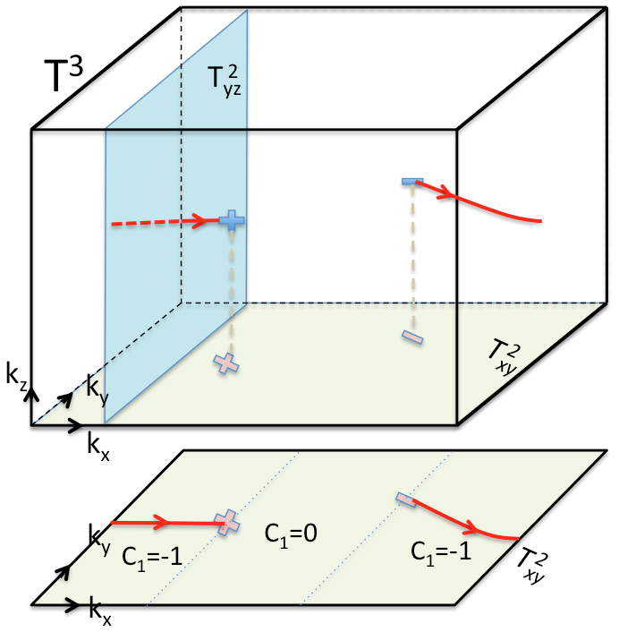
Refer to caption
Refer to caption
Figure 10. Red lines in the bulk Brillouin torus 𝕋3{\mathbb{T}}^{3} are Euler chains representing semimetals, encoding, in particular, how their first Chern numbers (weak invariants) c1yz,c1zxc_{1}^{yz},c_{1}^{zx} vary with kx,kyk_{x},k_{y}. Only the values of c1yzc_{1}^{yz} are indicated. Gapless surface states appear at points in the surface Brillouin torus 𝕋2{\mathbb{T}}^{2} where a first Chern number is non-zero, forming a Fermi arc connecting the projected Weyl points. The Fermi arc is determined from the Euler chain homologically by projection π\pi_{*}
Remark 3.6.

If we are able to access the complete specification of a semimetal Hamiltonian as an operator, then its surface Fermi arc is uniquely determined in principle. In practice, we have access to the Fermi arcs, and different Fermi arcs (as 1-chains) come from different Hamiltonians (as operators). The passage from Hamiltonian to Fermi arc can be modelled, for example, by transfer matrices [22, 4, 17]. At the topological level, a coarser but more appropriate question is how Fermi arcs may be used to distinguish topologically distinct semimetal Hamiltonians. For this latter question, we note that any Euler chain representative for a semimetal Hamiltonian HH maps under π\pi_{*} to a 1-chain which is topologically equivalent to the actual Fermi arc for HH. Thus Fermi arcs which are topologically distinct must come from topologically distinct Hamiltonians; our slight abuse of language in calling the 1-chain a “Fermi arc” does not matter at the level of topological invariants.

Certain scenarios involving tuning semimetal Hamiltonians and “rewiring” their surface Fermi arcs were considered in [36, 18]. These essentially involve homotopies 𝒉˘\breve{\bm{{h}}} which fix the local charges 𝒲=𝒲𝒉=𝒲𝒉\mathcal{W}=\mathcal{W}_{\bm{{h}}}=\mathcal{W}_{\bm{{h}}^{\prime}} (at least up to a diffeomorphism moving the Weyl points), and so induce the identity map on the class of Euler chains in 𝔈𝔲𝔩(T,𝒲)H1(T,W)\mathfrak{Eul}(T,\mathcal{W})\subset H_{1}(T,W). Under π\pi_{*}, the surface Fermi arcs for 𝒉\bm{{h}} and 𝒉\bm{{h}}^{\prime} may become “rewired”, but only in such a way that their class in H1(T~,W~)H_{1}(\widetilde{T},\widetilde{W}) remains unchanged. Rewirings which involve a change in H1(T~,W~)H_{1}(\widetilde{T},\widetilde{W}) necessarily require the prefiguring Euler chain in 𝔈𝔲𝔩(T,𝒲)\mathfrak{Eul}(T,\mathcal{W}) to change homology class, and this cannot be achieved by homotopies 𝒉˘\breve{\bm{{h}}} which fix the local charges 𝒲\mathcal{W}. Figures 11-12 illustrate some examples of rewirings.

Refer to caption
Figure 11. Black square represents 𝕋3{\mathbb{T}}^{3} with one coordinate suppressed; we can also interpret it as the projected surface Brillouin torus 𝕋2{\mathbb{T}}^{2}. Two homologous Euler chains (the left and right pairs of red directed lines) having the same local charge configuration are shown, and we can also interpret them as the corresponding surface Fermi arcs. [L] First Chern numbers for 2D subtori in the yzyz (resp. zxzx) directions at fixed kxk_{x} (resp. kyk_{y}) are shown, and may be computed by counting the signed intersection between the Euler chain and the subtorus. The “straightness” of the Euler chain does not matter, and Chern numbers can also be calculated for 2-cycles other than the standard 2D subtori with a fixed coordinate [R].
Refer to caption
Figure 12. More complicated Euler chains in 𝔈𝔲𝔩(T,𝒲)H1(𝕋3,W)\mathfrak{Eul}(T,\mathcal{W})\subset H_{1}({\mathbb{T}}^{3},W) representing more semimetal invariants in 𝔠𝔬𝔈𝔲𝔩(T,𝒲)H2(𝕋3W)\mathfrak{coEul}(T,\mathcal{W})\subset H^{2}({\mathbb{T}}^{3}\setminus W). The left and right Euler chains are not homologous.
Remark 3.7.

In d>3d>3, the intuition afforded by Figures 4 and 10-12 carries over in much the same way. For example, in d=4d=4, the blue surfaces represent hyperplane slices (3-tori) on which the semimetal gerbe of Section 4.6.1 restricts and has a curvature 3-form. There are four independent slice directions. As a slice is moved transversely across a semimetal band crossing with local charge qq, the Dixmier–Douady invariant of the gerbe on the slice jumps by qq. In d=5d=5, the slices are 4-tori and and it is the second Chern number of the 𝖳\mathsf{T}-invariant semimetal (Section 4.5) which jumps by qq.

Remark 3.8.

It is also possible to define Euler structures for TT even if χ(T)0\chi(T)\neq 0 by introducing a basepoint k0Tk_{0}\in T which “contains χ(T)\chi(T)”, see [12]. An Euler chain for a 0-chain 𝒲\mathcal{W} is then a 1-chain lC1(T,)l\in C_{1}(T,{\mathbb{Z}}) such that l=𝒲χ(T)k0\partial l=\mathcal{W}-\chi(T)k_{0}. Every vector field 𝒉\bm{{h}} on TT with isolated zeroes WW admits an Euler chain for its 0-chain 𝒲𝒉\mathcal{W}_{\bm{{h}}} of local charges in this sense: take l=wWIndw(𝒉)(wk0)l=\sum_{w\in W}\text{Ind}_{w}(\bm{{h}})(w-k_{0}), then l=wWIndw(𝒉)w(wWIndw(𝒉))k0=𝒲𝒉χ(T)k0\partial l=\sum_{w\in W}\text{Ind}_{w}(\bm{{h}})w-(\sum_{w\in W}\text{Ind}_{w}(\bm{{h}}))k_{0}=\mathcal{W}_{\bm{{h}}}-\chi(T)k_{0} by the Poincaré–Hopf theorem. Euler structures for TT with basepoint k0k_{0} are then defined as classes of pairs (𝒉,l)(\bm{{h}},l) which are considered equivalent if l2=l1+cs(𝒉1,𝒉2)l_{2}=l_{1}+\text{cs}(\bm{{h}}_{1},\bm{{h}}_{2}) up to a boundary. There is an action of H1(T,)H_{1}(T,{\mathbb{Z}}) on these classes by addition to ll, which is furthermore free and transitive.

4. Topological semimetal invariants in d=3,4,5d=3,4,5

4.1. General remarks on Bloch bundles and gauge invariance

Often, it is implicitly assumed that the Hamiltonians act on a trivial Bloch bundle 𝒮=T×n\mathscr{S}=T\times{\mathbb{C}}^{n} and that a trivialisation (choice of basis) has been given, so that the Dirac-type Hamiltonians of the form (2.1) are well-defined globally. Although this default setting suffices to illustrate many interesting features of semimetals, it is worth mentioning that non-trivial 𝒮\mathscr{S} can arise physically and can still be handled mathematically. In general one has, after a Bloch–Floquet transform, a Hilbert bundle T\mathscr{H}\rightarrow T in which the fibre k\mathscr{H}_{k} over kTk\in T comprises the quasi-periodic Bloch wavefunctions with quasimomentum kk [19, 54, 28, 32]. One typically restricts attention to a low-energy subbundle 𝒮\mathscr{S} defined by a finite number of energy bands separated from the rest by spectral gaps. Subsequently, a Bloch bundle 𝒮\mathscr{S} will refer to such a truncated finite-rank hermitian vector bundle over a manifold TT of (quasi)-momenta, on which the Bloch Hamiltonians act fiberwise.

In the theory of topological band insulators, it is crucial that 𝒮\mathscr{S} or its subbundles can be non-trivializable, e.g. 2D Chern insulators are essentially specified by the first Chern class of a non-trivializable valence line bundle. Expressions such as (2.1) should be understood as local expressions, which continue to make sense on a Bloch bundle 𝒮\mathscr{S} as long as 𝒮\mathscr{S} has the structure of a Clifford module bundle (or spinor bundle) so that the n×nn\times n operators γi\gamma_{i} are well-defined globally. In particular, the analysis of the spectrum of H=𝒉𝜸H=\bm{{h}}\cdot\bm{{\gamma}} remains the same for any 𝒮\mathscr{S} — namely, the ±|𝒉(k)|\pm|\bm{{h}}(k)| eigenspaces degenerate (i.e. there is a band crossing) precisely at the zeroes of 𝒉\bm{{h}}. On the other hand, the topology of the valence subbundle over TWT\setminus W, which is defined by the Fermi projection 12(1𝒉^(k))\frac{1}{2}(1-\hat{\bm{{h}}}(k)), does depend on 𝒮\mathscr{S} through the operators γi\gamma_{i}.

When n>2n>2, the most general nn-band Hamiltonian is not of Dirac-type, and well-defined topological invariants should respect the U(n)\text{U}(n) gauge invariance of the rank-nn Bloch bundle 𝒮\mathscr{S}. Nevertheless, Dirac-type Hamiltonians are generic when certain time-reversal/particle-hole symmetries are imposed. Such additional symmetries restrict the gauge group, and the topological invariants which we will define for insulators/semimetals described by Dirac-type Hamiltonians, are gauge invariant in this restricted sense. Some examples of such gauge restrictions were studied in [5, 6], and we also analyse them in Section 4.

4.2. General Hamiltonians over a manifold

The properties of Dirac-type Hamiltonians which are relevant for defining insulator/semimetal invariants can be abstracted as follows. An abstract (quantized) Dirac-type Hamiltonian is a section of the vector part of some Clifford algebra bundle over a momentum space manifold TT, i.e. the quantization of a vector field 𝒉\bm{{h}} specifying the abstract Hamiltonian as in Definition 2.1. Pointwise in TT, the spectrum of such a Hamiltonian (as a Clifford algebra element) can be found quite easily; it depends only on the vector field and has the crucial feature that it degenerates exactly at the zero set WW of the vector field. When such Hamiltonians are represented on some Clifford module bundle 𝒮\mathscr{S} (physically the Bloch bundle), they become concrete families of Hermitian operators with Fermi projections etc. The local topological invariant at a zero wWw\in W is intrinsic to 𝒉\bm{{h}} rather than the particular choice of Bloch bundle 𝒮\mathscr{S}, and exists even when 𝒮\mathscr{S} is not a trivial bundle. Furthermore, the symmetries and gauge structure for the Hamiltonians become more transparent at this abstract level, and this is especially so in higher dimensions.

Hamiltonians as quantized vector fields. For d3d\geq 3, let \mathcal{E} be an oriented rank-dd real vector bundle over a compact oriented manifold TT with fibre metric gg, along with a spinc structure (e.g. take TT a spinc manifold and \mathcal{E} its tangent bundle, then there is a H2(T,)H^{2}(T,{\mathbb{Z}}) worth of spinc structures to choose from). The Clifford algebra bundle Cl(,g)Cl(\mathcal{E},g) is a “quantization” of the exterior algebra bundle \bigwedge^{*}\mathcal{E} to allow for multiplication of vectors, both bundles having structure group SO(d)\text{SO}(d) [33]. With the spinc structure, we can construct the (irreducible) spinor bundle 𝒮\mathscr{S} (the “Bloch bundle”) of complex rank n=2d2n=2^{\lfloor\frac{d}{2}\rfloor}, with Spinc(d)\text{Spin}^{c}(d)-invariant Hermitian inner product, and Clifford multiplication gives a real bundle homomorphism Cl(,g)End(𝒮)Cl(\mathcal{E},g)\rightarrow\text{End}(\mathscr{S}). Thus there is a map c~:Cl(,g)End(𝒮)\tilde{c}:\bigwedge^{*}\mathcal{E}\rightarrow Cl(\mathcal{E},g)\rightarrow\text{End}(\mathscr{S}).

In particular, \mathcal{E}\subset\bigwedge^{*}\mathcal{E} is identified with a subbundle of Cl(,g)Cl(\mathcal{E},g), and the map c~\tilde{c} takes a section 𝒉Γ()\bm{{h}}\in\Gamma(\mathcal{E}) to a concrete Dirac-type Hamiltonian. More explicitly, an orthonormal frame {e1,,ed}\{e_{1},\ldots,e_{d}\} for \mathcal{E} becomes {c(e1),,c(ed)}\{c(e_{1}),\ldots,c(e_{d})\} in Cl(,g)Cl(\mathcal{E},g) and satisfies the Clifford relations c(ei)c(ej)+c(ej)c(ei)=2δijc(e_{i})c(e_{j})+c(e_{j})c(e_{i})=2\delta_{ij}. The c(ei)c(e_{i}) are represented on 𝒮\mathscr{S} as traceless self-adjoint endomorphisms c~(ei)γi\tilde{c}(e_{i})\equiv\gamma_{i} which inherit the familiar relations γiγj+γjγi=2δij𝟏𝒮\gamma_{i}\gamma_{j}+\gamma_{j}\gamma_{i}=2\delta_{ij}{\bf 1}_{\mathscr{S}}. Thus, a section 𝒉Γ()\bm{{h}}\in\Gamma(\mathcal{E}) defines a (quantized) abstract Dirac-type Hamiltonian c(𝒉)Γ(Cl(,g))c(\bm{{h}})\in\Gamma(Cl(\mathcal{E},g)) (c.f. Definition 2.1), which is then represented by a concrete Dirac-type Hamiltonian c~(𝒉)=𝒉𝜸\tilde{c}(\bm{{h}})=\bm{{h}}\cdot\bm{{\gamma}} acting on 𝒮\mathscr{S}. The concrete Dirac-type Bloch Hamiltonian above a point kTk\in T is the operator H(k)=𝒉(k)𝜸(k)H(k)=\bm{{h}}(k)\cdot\bm{{\gamma}}(k) acting on the fiber 𝒮kn\mathscr{S}_{k}\cong{\mathbb{C}}^{n}.

In the Clifford algebra bundle, it is already (SO(d)\text{SO}(d)-invariantly) true that c(𝒉)2=g(𝒉,𝒉)=|𝒉|2c(\bm{{h}})^{2}=g(\bm{{h}},\bm{{h}})=|\bm{{h}}|^{2}. It follows that the spectrum of a Bloch Hamiltonian is spec(H(k))=±|𝒉(k)|\text{spec}(H(k))=\pm|\bm{{h}}(k)| with each eigenvalue 2d212^{\lfloor\frac{d}{2}\rfloor-1}-fold degenerate, independently of 𝒮\mathscr{S}, and this is Spinc(d)\text{Spin}^{c}(d)-invariant. Precisely at the zeroes of 𝒉\bm{{h}}, the two 2d212^{\lfloor\frac{d}{2}\rfloor-1}-fold degenerate energy bands cross, and such a crossing is precisely protected by the topological index of 𝒉\bm{{h}} there.

More generally, we only require 𝒮\mathscr{S} to be a Clifford module bundle for Cl(,g)Cl(\mathcal{E},g), for which c(𝒉)Γ(Cl(,g))c(\bm{{h}})\in\Gamma(Cl(\mathcal{E},g)) acts self-adjointly. Such Clifford module bundles are in fact twisted versions of spinor bundles, obtained by tensoring with some vector bundle 𝒱\mathcal{V}, so we shall mainly consider only irreducible spinor bundles. In Section 5 we will also consider 2Cl(,g)\bigwedge^{2}\mathcal{E}\subset Cl(\mathcal{E},g) acting skew-adjointly on 𝒮\mathscr{S}, giving rise to “bilinear Hamiltonians”.

Remark 4.1.

Physically, one might start off with a given Bloch bundle 𝒮\mathscr{S}, which is a hermitian U(n)\text{U}(n) vector bundle over TT obtained by Fourier/Bloch–Floquet transform. In order to have a notion of Clifford multiplication and Dirac-type Hamiltonians, we need some assumptions on 𝒮\mathscr{S} allowing it to have the structure of a (irreducible) Clifford module bundle for some \mathcal{E}. In the first place, 𝒮\mathscr{S} should have the correct (complex) rank. In most model Hamiltonians considered in the physics literature, T=𝕋dT={\mathbb{T}}^{d} and the Bloch bundle 𝒮\mathscr{S} is assumed to be trivial. In this case, we take the trivial bundle \mathcal{E}, identified with the tangent bundle of 𝕋d{\mathbb{T}}^{d}, and 𝒉Γ()\bm{{h}}\in\Gamma(\mathcal{E}) is a tangent vector field. Then the corresponding Dirac-type Bloch Hamiltonian H(k)=𝒉(k)𝜸H(k)=\bm{{h}}(k)\cdot\bm{{\gamma}} has gamma matrices γi\gamma_{i} which can be taken to be constant over 𝕋d{\mathbb{T}}^{d}.

4.3. Remarks on 𝖳\mathsf{T} and 𝖢\mathsf{C} symmetries

Formally, a family of n×nn\times n Bloch Hamiltonians over TT can also be regarded as a family of Hamiltonians on an nn-level quantum mechanical system, with adiabatic phases/holonomies, etc. There is, however, a fundamental difference between TT as an adiabatic parameter space and as a quasi-momentum space, when antiunitary symmetries are introduced. The Brillouin torus 𝕋d{\mathbb{T}}^{d} is topologically the space of unitary characters for the translation group d{\mathbb{Z}}^{d} of a lattice, so the complex conjugation involved in an antiunitary symmetry operator induces an involution τ\tau (a 2{\mathbb{Z}}_{2}-action) on 𝕋d{\mathbb{T}}^{d}. Explicitly, when we parameterise 𝕋d{\mathbb{T}}^{d} by angles k=(k1,,kd)k=(k_{1},\ldots,k_{d}), the character neinkn\mapsto e^{\text{i}n\cdot k} labelled by kk conjugates to the character labelled by kτ(k)-k\equiv\tau(k). In the context of Bloch Hamiltonians, a fermionic time-reversal symmetry 𝖳\mathsf{T} is a lift of τ\tau to a map on the Bloch bundle 𝒮\mathscr{S} which is antiunitary on fibres, and satisfies 𝖳2=1\mathsf{T}^{2}=-1. Compatibility of 𝖳\mathsf{T} with H(k),k𝕋dH(k),k\in{\mathbb{T}}^{d} is then the condition 𝖳(k)H(k)𝖳(k)1=H(τ(k))\mathsf{T}(k)H(k)\mathsf{T}(k)^{-1}=H(\tau(k)). Such bundles equipped with a “Quaternionic” structure 𝖳\mathsf{T} were studied in [16], and have more recently been investigated in the context of topological insulators [19, 15, 38, 62]. For bosonic time-reversal, 𝖳\mathsf{T} squares to the identity instead, and is sometimes called a “Real structure”.

Similarly, an antiunitary particle-hole symmetry 𝖢\mathsf{C} anticommutes with the Bloch Hamiltonians in a way that respects τ\tau, namely, 𝖢(k)H(k)𝖢(k)1=H(τ(k))\mathsf{C}(k)H(k)\mathsf{C}(k)^{-1}=-H(\tau(k)). On the other hand, for a family of Hamiltonians parametrised by TT, we simply have 𝖳(k)H(k)𝖳(k)1=H(k)\mathsf{T}(k)H(k)\mathsf{T}(k)^{-1}=H(k) and 𝖢(k)H(k)𝖢(k)1=H(k),kT\mathsf{C}(k)H(k)\mathsf{C}(k)^{-1}=-H(k),\,k\in T, without the involution τ\tau. In either case, the squares 𝖳2,𝖢2\mathsf{T}^{2},\mathsf{C}^{2} may be ±1\pm 1, and when both 𝖳\mathsf{T} and 𝖢\mathsf{C} are present, they may be assumed to commute [19].

The same involution τ\tau is induced on 𝕋d{\mathbb{T}}^{d} by a spatial inversion symmetry 𝖯\mathsf{P}, since a translation by ndn\in{\mathbb{Z}}^{d} becomes a translation by n-n. Thus we can consider a time-reversal symmetry which concurrently effects spatial inversion77 7 Note that this is not the same as requiring 𝖳\mathsf{T} and 𝖯\mathsf{P} to separately be symmetries, and indeed, the latter situation requires additional data specifying whether 𝖯,𝖳\mathsf{P},\mathsf{T} commute or anticommute [71, 58], leading in each case to different Wigner classes.; we write (𝖳𝖯)(\mathsf{T}\mathsf{P}) for such a symmetry operator. Then we have (𝖳𝖯(k))H(k)(𝖳𝖯(k))1=H(k),k𝕋d(\mathsf{T}\mathsf{P}(k))H(k)(\mathsf{T}\mathsf{P}(k))^{-1}=H(k),\,k\in{\mathbb{T}}^{d} where the effect of τ\tau now cancels; similarly for (𝖢𝖯)(\mathsf{C}\mathsf{P}). Thus the operator (𝖳𝖯)(\mathsf{T}\mathsf{P}) is an ordinary quaternionic structure, and the Bloch bundle 𝒮\mathscr{S} has invariants as a symplectic bundle.

Convention. For this paper, we will simply write 𝖳,𝖢\mathsf{T},\mathsf{C} with the understanding that (𝖳𝖯),(𝖢𝖯)(\mathsf{T}\mathsf{P}),(\mathsf{C}\mathsf{P}) is meant whenever TT is a Brillouin torus. Thus we always have 𝖳(k)H(k)𝖳(k)1=H(k)\mathsf{T}(k)H(k)\mathsf{T}(k)^{-1}=H(k) and 𝖢(k)H(k)𝖢(k)1=H(k),kT\mathsf{C}(k)H(k)\mathsf{C}(k)^{-1}=-H(k),\,k\in T.

4.4. Abstract Weyl semimetal in 3D

Let us explain the above abstractions in more detail for two-band Hamiltonians in d=3d=3, in which dim𝒮=2\text{dim}_{\mathbb{C}}\mathscr{S}=2. This is the setting for the basic Weyl semimetal.

Since Spinc(3)=U(2)\text{Spin}^{c}(3)=\text{U}(2), any rank-2 hermitian vector bundle 𝒮\mathscr{S} can arise as a spinor bundle: take the traceless Hermitian endomorphisms 0\mathcal{H}_{0} of 𝒮\mathscr{S} with the Hilbert–Schmidt real inner product H1(k),H2(k)=12tr(H1H2(k))\langle H_{1}(k),H_{2}(k)\rangle=\frac{1}{2}\text{tr}(H_{1}\circ H_{2}(k)). Then 0\mathcal{H}_{0} becomes a real orientable rank-3 bundle with structure group SO(3)=PU(2)\text{SO}(3)=\text{PU}(2) liftable to Spinc(3)\text{Spin}^{c}(3). An orthonormal frame for 0\mathcal{H}_{0} gives a set of Pauli operators {σ1,σ2,σ3}\{\sigma_{1},\sigma_{2},\sigma_{3}\}, which is positively oriented if σ1σ2=iσ3\sigma_{1}\sigma_{2}=\text{i}\sigma_{3}. Such a positively-oriented frame has the form of the standard Pauli matrices in some local trivialization of 𝒮\mathscr{S}. The Bloch Hamiltonian is given locally by H(k)=𝒉(k)𝝈H(k)=\bm{{h}}(k)\cdot\bm{{\sigma}}. Then (0,,)(\mathcal{H}_{0},\langle\cdot,\cdot\rangle) has a Clifford algebra bundle and a choice of spinc structure yields a spinor bundle. 𝒮\mathscr{S} is some twisted version of this spinor bundle, and the twisting can be thought of as changing the spinc structure under the canonical action of H2(T,)H^{2}(T,{\mathbb{Z}}) [33].

Thus {σ1,σ2,σ3}\{\sigma_{1},\sigma_{2},\sigma_{3}\} may be thought of as {c~(e1),c~(e2),c~(e3)}\{\tilde{c}(e_{1}),\tilde{c}(e_{2}),\tilde{c}(e_{3})\} for an orthonormal frame {e1,e2,e3}\{e_{1},e_{2},e_{3}\} in (,g)(0,,)(\mathcal{E},g)\cong(\mathcal{H}_{0},\langle\,\cdot\,,\,\cdot\,\rangle). From this point of view, a vector field 𝒉Γ()\bm{{h}}\in\Gamma(\mathcal{E}) is quantized to an abstract Hamiltonian c(𝒉)Cl(,g)c(\bm{{h}})\in Cl(\mathcal{E},g), which acts concretely as c~(𝒉)=𝒉𝝈\tilde{c}(\bm{{h}})=\bm{{h}}\cdot\bm{{\sigma}} on 𝒮\mathscr{S}. Note that, in particular, the spectrum spec(H(k))=±|𝒉(k)|\text{spec}(H(k))=\pm|\bm{{h}}(k)| is invariant under U(2)=Spinc(3)\text{U}(2)=\text{Spin}^{c}(3) gauge transformations of 𝒮\mathscr{S}.

Remark 4.2.

A gauge transformation of the Bloch bundle 𝒮\mathscr{S} implemented by local 2×22\times 2 unitaries U(k)U(k) turns 𝒉(k)𝝈\bm{{h}}(k)\cdot\bm{{\sigma}} into the conjugate U(k)(𝒉(k)𝝈)U1(k)U(k)(\bm{{h}}(k)\cdot\bm{{\sigma}})U^{-1}(k). The result of this conjugation is known to be equal to 𝒉(k)σ\bm{{h^{\prime}}}(k)\cdot\sigma where 𝒉(k)\bm{{h^{\prime}}}(k) is rotated from 𝒉(k)\bm{{h}}(k) by the SO(3)\text{SO}(3) element π(U(k))\pi(U(k)) in

1U(1)U(2)𝜋PU(2)=SO(3)1.1\rightarrow\text{U}(1)\rightarrow\text{U}(2)\xrightarrow{\pi}\text{PU}(2)=\text{SO}(3)\rightarrow 1.

Similarly, PSU(2)=SO(3)\text{PSU}(2)=\text{SO}(3) in case the structure group of 𝒮\mathscr{S} can be reduced to SU(2)\text{SU}(2).

4.4.1. Symmetries of 3D semimetal

Two band-Hamiltonians can more generally include a trace term, i.e. H(k)=m(k)+𝒉(k)𝝈(k)H(k)=m(k)+\bm{{h}}(k)\cdot\bm{{\sigma}}(k), where m(k)m(k) is not constant and so not eliminable by shifting the overall energy level. Indeed, Hamiltonians with such m(k)m(k) terms (and constant 𝝈\bm{{\sigma}}) can give rise to new phenomena such as “Type-II Weyl semimetals” [75, 57]. It is possible to distinguish the two situations, i.e. eliminate the m(k)m(k) term, by imposing a natural symmetry constraint.

Quaternionic structure and 𝖢\mathsf{C}-symmetry. Let us recall the construction of the spinor representation SS of Cl0,3Cl_{0,3}. Let e1,e2,e3e_{1},e_{2},e_{3} be orthonormal vectors in 3{\mathbb{R}}^{3}, eiejeiejΛ2(3)e_{i}e_{j}\equiv e_{i}\wedge e_{j}\in\Lambda^{2}({\mathbb{R}}^{3}), and e1e2e3e1e2e3Λ3(3)e_{1}e_{2}e_{3}\equiv e_{1}\wedge e_{2}\wedge e_{3}\in\Lambda^{3}({\mathbb{R}}^{3}). The even part Cl0,3+Cl2,0Cl_{0,3}^{+}\cong Cl_{2,0} is isomorphic to {\mathbb{H}}, and for the complexified algebras, l3+l2M2()={\mathbb{C}}l_{3}^{+}\cong{\mathbb{C}}l_{2}\cong M_{2}({\mathbb{C}})={\mathbb{H}}\otimes_{\mathbb{R}}{\mathbb{C}}. The spinor representation on S=2S={\mathbb{C}}^{2} is the (unique complex) irreducible representation of l3+M2(){\mathbb{C}}l_{3}^{+}\cong M_{2}({\mathbb{C}}), and is extended to l3Cl0,3{\mathbb{C}}l_{3}\supset Cl_{0,3} by setting a chirality condition c~(ie1e2e3)=1\tilde{c}(-\text{i}e_{1}e_{2}e_{3})=1. Spin(3)=SU(2)Sp(1)\text{Spin}(3)=\text{SU}(2)\cong\text{Sp}(1) lies in Cl0,3+Cl_{0,3}^{+}\cong{\mathbb{H}} as the unit quaternions, and SS is an irreducible representation of Spin(3)\text{Spin}(3). This is just the fundamental representation of SU(2)Sp(1)\text{SU}(2)\cong\text{Sp}(1) which is well-known to be quaternionic.

The quantized bivectors c(e3e1),c(e3e2)c(e_{3}e_{1}),c(e_{3}e_{2}) generate Cl2,0Cl0,3+Cl_{2,0}\cong Cl^{+}_{0,3}\cong{\mathbb{H}}. On SS, they are represented by skew-Hermitian operators c~(e3e1)=iσ2,c~(e3e2)=iσ1\tilde{c}(e_{3}e_{1})=\text{i}\sigma_{2},\,\tilde{c}(e_{3}e_{2})=-\text{i}\sigma_{1} (which generate a quaternion algebra), and with the chirality element c~(ie1e2e3)\tilde{c}(-\text{i}e_{1}e_{2}e_{3}) being the identity operator on SS, we recover the Pauli matrices c~(ei)=σi\tilde{c}(e_{i})=\sigma_{i}. Since SS is a quaternionic representation for Spin(3)\text{Spin}(3), there is an antiunitary operator Θ\mathsf{\Theta} on SS commuting with Cl0,3+Spin(3)Cl^{+}_{0,3}\supset\text{Spin}(3) such that Θ2=1\mathsf{\Theta}^{2}=-1, from which we deduce that Θ\mathsf{\Theta} anticommutes with c(ei)=σic(e_{i})=\sigma_{i}. For instance, we can take Θ=iσ2κ\mathsf{\Theta}=\text{i}\sigma_{2}\circ\kappa where κ\kappa is complex conjugation in the basis where σi\sigma_{i} are the standard Pauli matrices. This operator is often taken to be the fermionic time-reversal operator 𝖳\mathsf{T} on spin-12\frac{1}{2} systems.

If \mathcal{E} has a spin (not just spinc) structure, there is also a notion of spinor bundles 𝒮\mathscr{S} associated to the spin structure [33], and these have structure group Spin(3)=SU(2)=Sp(1)\text{Spin}(3)=\text{SU}(2)=\text{Sp}(1). Globalising the above constructions, these spinor bundles come with a quaternionic structure 𝖢\mathsf{C} anticommuting with H=c~(𝒉)=𝒉𝝈H=\tilde{c}(\bm{{h}})=\bm{{h}}\cdot\bm{{\sigma}}.

Reduction to SU(2)Sp(1)\text{SU}(2)\cong\text{Sp}(1). Suppose we have a reduction of the structure group of the Bloch bundle from U(2)\text{U}(2) to Spin(3)=SU(2)\text{Spin}(3)=\text{SU}(2). This is possible exactly when det(𝒮)\text{det}(\mathscr{S}) is trivial, i.e. c1(𝒮)=c1(det(𝒮))=0c_{1}(\mathscr{S})=c_{1}(\text{det}(\mathscr{S}))=0 (this is a general result about reducing from U(n)\text{U}(n) to SU(n)\text{SU}(n)). Alternatively, since SU(2)=Sp(1)\text{SU}(2)=\text{Sp}(1), the reduction from U(2)\text{U}(2) to SU(2)\text{SU}(2) requires a quaternionic structure on 𝒮\mathscr{S}, which provides an isomorphism between the line bundles 1\mathcal{L}_{1} and 2¯\overline{\mathcal{L}_{2}} for an orthogonal splitting 𝒮=12\mathscr{S}=\mathcal{L}_{1}\oplus\mathcal{L}_{2}. Then c1(𝒮)=c1(1)+c1(2)=c1(1)c1(1)=0c_{1}(\mathscr{S})=c_{1}(\mathcal{L}_{1})+c_{1}(\mathcal{L}_{2})=c_{1}(\mathcal{L}_{1})-c_{1}(\mathcal{L}_{1})=0. In this case, we can identify 0\mathcal{H}_{0} with the tangent bundle 𝕋3\mathcal{E}\rightarrow{\mathbb{T}}^{3}, as (trivial) SO(3)\text{SO}(3) bundles.

Therefore, in the two-band case in 3D, the imposition of a 𝖢\mathsf{C}-symmetry constraint is one possible way to justify (1) the restriction from arbitrary 2×22\times 2 Bloch Hamiltonians to the traceless ones, and (2) the triviality of the Bloch bundle 𝒮\mathscr{S}.

4.5. 𝖳\mathsf{T}-invariant Dirac-semimetal in 5D

We now generalize the two-band crossings of the previous section to four-band crossings. These should involve crossings of pairs of bands, in analogy to the dispersion of massless Dirac spinors. Again, the adjective “Dirac” is loaded and possibly misleading, and our constructions below are more analogous to Weyl fermions in 1+5 D (which is still misleading). For this Subsection, we take TT to be a compact oriented 5-manifold, and 𝒮=T×4\mathscr{S}=T\times{\mathbb{C}}^{4} a trivial Hermitian vector bundle.

The bundle 0\mathcal{H}_{0} of traceless Hermitian endomorphisms of 𝒮\mathscr{S} is now a trivial rank-15 real vector bundle whose sections are Bloch Hamiltonians kH(k)k\mapsto H(k) with inner product H1(k),H2(k)=14tr(H1(k)H2(k))\langle H_{1}(k),H_{2}(k)\rangle=\frac{1}{4}\text{tr}(H_{1}(k)\circ H_{2}(k)).

For notational ease, we will sometimes suppress the dependence on kk when dealing with a single operator.

4.5.1. Dirac-type Hamiltonians in 5D

Physicists often restrict attention to “Dirac-type” Hamiltonians H(k)=𝒉(k)𝜸H(k)=\bm{{h}}(k)\cdot\bm{{\gamma}} where 𝜸={γ1,,γ5}\bm{{\gamma}}=\{\gamma_{1},\ldots,\gamma_{5}\} is an orthonormal set of 4×44\times 4 hermitian operators on SS satisfying the Clifford algebra relation γiγj+γjγi=2δij\gamma_{i}\gamma_{j}+\gamma_{j}\gamma_{i}=2\delta_{ij}, and 𝒉\bm{{h}} is a 5-component vector field. The pragmatic justification is ease of manipulation, since the spectrum is again easily found to be ±|𝒉(k)|\pm|\bm{{h}}(k)|, with doubly-degenerate eigenvalues that become four-fold degenerate precisely at the zeroes of 𝒉\bm{{h}} (Fig. 13). However, we should note that arbitrary gauge transformations will not preserve this particular form of 4×44\times 4 Hermitian matrices. It is therefore useful to find a symmetry which reduces the allowed gauge transformations so that the Dirac-form of HH is automatically preserved.

Refer to caption
Figure 13. Four-band crossings for Dirac-type Hamiltonians, with symmetric spectrum.

We do this by invoking a 𝖳\mathsf{T}-symmetry constraint (a quaternionic structure) on the Hamiltonians, which will pick out the Dirac-type Hamiltonians as a rank-5 subbundle of 0\mathcal{H}_{0}. In fact, the observation that the proper gauge groups and Berry connections/phases for time-reversal invariant Hamiltonians are quaternionic, had already been made in [5, 6, 23], and in the 4×44\times 4 case such Hamiltonians can be constructed by considering 4{\mathbb{C}}^{4} as a spin-32\frac{3}{2} representation (so-called “quadrupole Hamiltonians”). We give a more direct account, emphasizing the Clifford algebra and spin groups responsible for this structure.

Consider first a fibre 422{\mathbb{C}}^{4}\cong{\mathbb{C}}^{2}\otimes{\mathbb{C}}^{2} and define the antiunitary operator

(4.1) Θ=(1iσ2)κ,\Theta=(1\otimes\text{i}\sigma_{2})\circ\kappa,

where κ\kappa is complex conjugation, which satisfies Θ2=1\Theta^{2}=-1. We verify that (real) linear combinations of the following mutually anticommuting γi,i=1,,5\gamma_{i},i=1,\ldots,5, commute with Θ\Theta:

(4.2) γ1=σ2σ1,γ2=σ2σ2,γ3=σ2σ3,γ4=σ11,γ5=σ31.\gamma_{1}=\sigma_{2}\otimes\sigma_{1},\quad\gamma_{2}=\sigma_{2}\otimes\sigma_{2},\quad\gamma_{3}=\sigma_{2}\otimes\sigma_{3},\quad\gamma_{4}=\sigma_{1}\otimes 1,\quad\gamma_{5}=\sigma_{3}\otimes 1.

A more invariant way to see this is to notice that an anticommuting set of 4×44\times 4 Hermitian operators γ1,,γ4\gamma_{1},\ldots,\gamma_{4} satisfying γiγj+γjγi=2δij,i,j=1,,4\gamma_{i}\gamma_{j}+\gamma_{j}\gamma_{i}=2\delta_{ij},i,j=1,\ldots,4, generate (over the reals) a copy of Cl0,4M2()Cl_{0,4}\cong M_{2}({\mathbb{H}}) inside M4()M_{4}({\mathbb{C}}) which thereby commutes with a opp{\mathbb{H}}^{\text{opp}} action generated by i,Θ\text{i},\Theta (two anticommuting square roots of 1-1). The product of two or three different γi,i=1,,4\gamma_{i},\,i=1,\ldots,4 is not Hermitian, but γ5=γ1γ2γ3γ4\gamma_{5}=\gamma_{1}\gamma_{2}\gamma_{3}\gamma_{4} is Hermitian and also commutes with Θ\Theta. The remaining ten-dimensional subspace of traceless Hermitian operators is spanned by operators iγiγj,ij\text{i}\gamma_{i}\gamma_{j},i\neq j and they anticommute with Θ\Theta instead — we will interpret this latter subspace of 4×44\times 4 Hamiltonians as those compatible with a particle-hole symmetry 𝖢\mathsf{C}, and these form an important class to be analysed in Section 5.2.

Therefore, traceless Hermitian operators of the form H=𝒉𝜸H=\bm{{h}}\cdot\bm{{\gamma}} are precisely those which are compatible with a quaternionic structure Θ\Theta, which we interpret as a time-reversal operator 𝖳\mathsf{T}. Conversely, a quaternionic structure Θ\Theta identifies 4{\mathbb{C}}^{4} with 2{\mathbb{H}}^{2}, and M2()Cl0,4M_{2}({\mathbb{H}})\cong Cl_{0,4} is the real subalgebra of M2()M_{2}({\mathbb{C}}) which commutes with Θ\Theta.

Globalising the above arguments, we deduce:

Proposition 4.3.

A quaternionic structure Θ\Theta on a rank-44 Bloch bundle picks out a real orientable rank-5 subbundle 0,l0\mathcal{H}_{0,l}\subset\mathcal{H}_{0} of commuting Dirac-type Hamiltonians. The chirality condition γ5=γ1γ2γ3γ4\gamma_{5}=\gamma_{1}\gamma_{2}\gamma_{3}\gamma_{4} for an orthonormal frame {γ1,,γ5}\{\gamma_{1},\ldots,\gamma_{5}\} for 0,l\mathcal{H}_{0,l} defines the positive orientation.

A quaternionic structure always exists on a trivial Bloch bundle, and in this case, we identify 0,l\mathcal{H}_{0,l} with the tangent bundle \mathcal{E} as SO(5)\text{SO}(5)-bundles. Thus {γ1,,γ5}\{\gamma_{1},\dots,\gamma_{5}\} corresponds to a positively-oriented orthonormal frame {e1,,e5}\{e_{1},\ldots,e_{5}\} for \mathcal{E}. In terms of Clifford modules, the Clifford algebra Cl0,5Cl_{0,5} has S=4S={\mathbb{C}}^{4} as the spinor representation in which the central chirality element c~(e1e2e3e4e5)\tilde{c}(e_{1}e_{2}e_{3}e_{4}e_{5}) is the identity operator. A vector field 𝒉\bm{{h}} is quantized to an abstract Dirac-type Hamiltonian c(𝒉)c(\bm{{h}}), which is represented concretely on 𝒮\mathscr{S} as the Hamiltonian H=c~(𝒉)=𝒉𝜸=i=15hiγiH=\tilde{c}(\bm{{h}})=\bm{{h}}\cdot\bm{{\gamma}}=\sum_{i=1}^{5}h^{i}\gamma_{i} isometrically: 𝒉1,𝒉2=14tr(𝒉1𝒉2+)=𝒉1𝒉2\langle{\bm{{h}}_{1},\bm{{h}}_{2}}\rangle=\frac{1}{4}\text{tr}(\bm{{h}}_{1}\cdot\bm{{h}}_{2}+\ldots)=\bm{{h}}_{1}\cdot\bm{{h}}_{2}.

Remark 4.4.

The observation that the space 0,l\mathcal{H}_{0,l} has structure group SO(5)\text{SO}(5) was made in Section 5 of [6] (for trivial bundles 𝒮\mathscr{S}). Generalizing Remark 4.2, SS is the spinor representation for Spin(5)Sp(2)U(4)\text{Spin}(5)\cong\text{Sp}(2)\subset\text{U}(4), and conjugating H(k)=𝒉(k)𝜸H(k)=\bm{{h}}(k)\cdot\bm{{\gamma}} by a Spin(5)\text{Spin}(5) unitary matrix U(k)U(k) takes it to H(k)=𝒉(k)𝜸H^{\prime}(k)=\bm{{h}}^{\prime}(k)\cdot\bm{{\gamma}} where 𝒉(k)\bm{{h}}^{\prime}(k) is rotated from 𝒉(k)\bm{{h}}(k) by the SO(5)\text{SO}(5) matrix R(k)R(k) covered by U(k)U(k). The reduction of the gauge group is important: to stay within the class of Dirac-type Hamiltonians, we cannot allow all U(4)\text{U}(4) gauge transformations of the Bloch bundle 𝒮\mathscr{S}, but only those in Spin(5)Sp(2)\text{Spin}(5)\cong\text{Sp}(2).

4.5.2. Quaternionic valence line bundle, local {\mathbb{Z}}-charge, and second Chern class

For a 5-component vector field with finite isolated zeroes WTW\subset T, the local index at wWw\in W is again given by the degree of the unit vector map 𝒉^:Sw4S45\hat{\bm{{h}}}:S^{4}_{w}\rightarrow S^{4}\subset{\mathbb{R}}^{5} restricted to a small sphere around ww. This {\mathbb{Z}}-valued local index measures the obstruction to “gapping” out a four-band crossing within the family of Dirac-type Hamiltonians (or 𝖳\mathsf{T}-invariant Hamiltonians). Away from WW, H(k)H(k) can be spectrally-flattened to sgn(H(k))=𝒉^(k)𝜸\text{sgn}(H(k))=\hat{\bm{{h}}}(k)\cdot\bm{{\gamma}}, and the Fermi projection 12(1sgn(H(k))CLOSE\frac{1}{2}(1-\text{sgn}(H(k)) projects onto a complex rank-2 subspace of S=4S={\mathbb{C}}^{4}. This subspace is actually a quaternionic line, i.e. an element of 1{\mathbb{H}}{\mathbb{P}}^{1}, due to the existence of Θ\Theta commuting with H(k)H(k). Just as a unit 3-vector defines a point in 1S2{\mathbb{C}}{\mathbb{P}}^{1}\cong S^{2} via 𝒉\bm{{h}}\leftrightarrow (1)(-1)-subspace of 𝒉𝝈\bm{{h}}\cdot\bm{{\sigma}}, we also have 1S4{\mathbb{H}}{\mathbb{P}}^{1}\cong S^{4} via {unit 5-vector 𝒉\bm{{h}}} \leftrightarrow {(1)(-1)-subspace of 𝒉𝜸\bm{{h}}\cdot\bm{{\gamma}}}.

The valence subbundle F\mathcal{E}_{F} of a 𝖳\mathsf{T}-invariant Dirac-type Hamiltonian in 5D is thus a quaternionic line bundle over TWT\setminus W. These quaternionic line bundles are pulled back from the tautological one over 1=S4{\mathbb{H}}{\mathbb{P}}^{1}=S^{4}, and may have non-trivial symplectic Pontryagin class/second Chern class in H4(,)H^{4}(\,\cdot\,,{\mathbb{Z}}) [7, 5].

Remark 4.5.

The symplectic Pontryagin classes qiq_{i} for Sp(n)\text{Sp}(n) bundles [7], should be distinguished from the real Pontryagin classes pip_{i} for O(n) bundles. The former comes from H4i(BSp(n),)H^{4i}(\text{BSp}(n),{\mathbb{Z}}) and equals (1)ic2i(-1)^{i}c_{2i} of the underlying complex bundle of a quaternionic bundle, while the latter comes from H4i(BO(n),)H^{4i}(\text{BO}(n),{\mathbb{Z}}) and equals (1)ic2i(-1)^{i}c_{2i} of the complexification of the underlying real bundle of a complex bundle (e.g. underlying a quaternionic one). For the tautological quaternionic line bundle 1\mathcal{H}\rightarrow{\mathbb{H}}{\mathbb{P}}^{1}, the symplectic Pontryagin class/second Chern class is a generator of H4(S4,)=H^{4}(S^{4},{\mathbb{Z}})={\mathbb{Z}}.

The H4H^{4} part of the semimetal Mayer–Vietoris sequence

(4.3) 0H4(T)ιH4(TW)𝛽H4(SW4)ΣH5(T)0\cdots 0\rightarrow H^{4}(T)\xrightarrow{\iota^{*}}H^{4}(T\setminus W)\xrightarrow{\beta}H^{4}(S^{4}_{W})\xrightarrow{\Sigma}H^{5}(T)\rightarrow 0\ldots

is slightly harder to interpret in terms of characteristic classes of F\mathcal{E}_{F}: unlike H2(,)H^{2}(\cdot,{\mathbb{Z}}) and complex line bundles, it is not generally true that H4(,)H^{4}(\cdot,{\mathbb{Z}}) classifies all quaternionic line bundles (equivalently Sp(1)=SU(2)\text{Sp}(1)=\text{SU}(2)-bundles) over a given space. For example, SU(3)\text{SU}(3) is a non-trivial SU(2)\text{SU}(2) bundle over S5S^{5} but H4(S5,)=0H^{4}(S^{5},{\mathbb{Z}})=0 so c2c_{2} doesn’t detect this bundle. Nevertheless, H4(𝕋5,)5H^{4}({\mathbb{T}}^{5},{\mathbb{Z}})\cong{\mathbb{Z}}^{5} with the generators coming from pulling back \mathcal{H} along the projection 𝒉:𝕋5𝕋4S4=1\bm{{h}}:{\mathbb{T}}^{5}\rightarrow{\mathbb{T}}^{4}\rightarrow S^{4}={\mathbb{H}}{\mathbb{P}}^{1} for each of the five independent choices of 4-subtori. Thus all elements of H4(𝕋5,)H^{4}({\mathbb{T}}^{5},{\mathbb{Z}}) do arise as the second Chern class of some valence quaternionic line bundle F𝕋5\mathcal{E}_{F}\rightarrow{\mathbb{T}}^{5} (weak insulator invariants), and their restrictions to H4(𝕋5W)H^{4}({\mathbb{T}}^{5}\setminus W) form the kernel of the local charge map β\beta in (4.3). The other elements ωH4(𝕋5W)\omega\in H^{4}({\mathbb{T}}^{5}\setminus W) have some non-zero local charges under β\beta. From a singular vector field 𝒉\bm{{h}} with those local charges β(ω)\beta(\omega), the valence bundle for 𝒉𝜸\bm{{h}}\cdot\bm{{\gamma}} has c2(F)=ωc_{2}(\mathcal{E}_{F})=\omega. Thus for T=𝕋5T={\mathbb{T}}^{5}, the H4(,)H^{4}(\cdot,{\mathbb{Z}}) groups in (4.3) can be interpreted as the weak invariants c2c_{2} for the valence bundles F\mathcal{E}_{F} of the Dirac-type Hamiltonians as constructed above.

Remark 4.6.

Quaternionic line bundles are already stable for dim(T)=5(T)=5 [3], so we can classify the F\mathcal{E}_{F} by (reduced) quaternionic KK-theory KSpKSp. Therefore, the semimetal MV-sequence in KSpKSp can be interpreted in terms of obstructions to extending a semimetal valence bundle (over 𝕋5W{\mathbb{T}}^{5}\setminus W) to an insulator one (over 𝕋5{\mathbb{T}}^{5}).

4.6. 𝖳\mathsf{T}-invariant and chiral symmetric Dirac-semimetal in 4D

When we introduced 𝖳\mathsf{T} to 4×44\times 4 Hamiltonians, we found that they had the form H(k)=𝒉(k)𝜸H(k)=\bm{{h}}(k)\cdot\bm{{\gamma}} for some 5-component vector 𝒉(k)\bm{{h}}(k). Now introduce a further (unitary) chiral symmetry 𝖲\mathsf{S}, with 𝖲2=1,𝖲𝖳=𝖳𝖲\mathsf{S}^{2}=1,\mathsf{S}\mathsf{T}=\mathsf{T}\mathsf{S} which a compatible HH must anticommute with. Without loss, we can take 𝖲=γ5\mathsf{S}=\gamma_{5}. Equivalently, this is an additional (antiunitary) 𝖢\mathsf{C} symmetry, with 𝖢𝖳=𝖳𝖢\mathsf{C}\mathsf{T}=\mathsf{T}\mathsf{C} and 𝖢2=1\mathsf{C}^{2}=-1: take 𝖢=(σ3iσ2)κ=𝖳𝖲\mathsf{C}=(-\sigma_{3}\otimes\text{i}\sigma_{2})\circ\kappa=-\mathsf{T}\circ\mathsf{S}. The additional anticommutation requirement 𝖲H=H𝖲\mathsf{S}H=-H\mathsf{S} (or 𝖢H=H𝖢\mathsf{C}H=-H\mathsf{C}) forces H(k)H(k) to be a linear combination of only the first four gamma matrices in (4.2). Furthermore, the traceless condition on HH is now automatic.

Thus in 4D, we may identify the (𝖳,𝖢)(\mathsf{T},\mathsf{C})-compatible (or (𝖳,𝖲)(\mathsf{T},\mathsf{S})-compatible) 4×44\times 4 Hamiltonians with the tangent bundle of 𝕋4{\mathbb{T}}^{4}, via H(k)=𝒉(k)𝜸H(k)=\bm{{h}}(k)\cdot\bm{{\gamma}}, where 𝒉,𝜸\bm{{h}},\bm{{\gamma}} now have four components. Similarly, S=4S={\mathbb{C}}^{4} is the spinor representation for Cl0,4M4()Cl_{0,4}\otimes_{\mathbb{R}}{\mathbb{C}}\cong M_{4}({\mathbb{C}}) which has a quaternionic structure Θ=𝖳\Theta=\mathsf{T} compatible with Cl0,4=M2()Cl_{0,4}=M_{2}({\mathbb{H}}). The spectrum is again spec(H(k))=±|𝒉(k)|\text{spec}(H(k))=\pm|\bm{{h}}(k)|, vanishing at the zeroes W𝕋4W\subset{\mathbb{T}}^{4} of 𝒉\bm{{h}}. The topological invariant for a four-band crossing at a zero wWw\in W is the degree of the unit vector map 𝒉^:Sw3S34\hat{\bm{{h}}}:S_{w}^{3}\rightarrow S^{3}\in{\mathbb{R}}^{4}.

Remark 4.7.

There is also an analysis based on supercommutants. The requirement of having symmetry operators 𝖳,𝖢\mathsf{T},\mathsf{C} is equivalent to having a 2{\mathbb{Z}}_{2}-graded representation of the Clifford algebra Cl3,0Cl_{3,0}𝖢,i𝖢,i𝖢𝖳\mathsf{C},\text{i}\mathsf{C},\text{i}\mathsf{C}\mathsf{T} are the three anticommuting Clifford generators, acting irreducibly as odd operators on the superspace 4=1|1{\mathbb{C}}^{4}={\mathbb{H}}\otimes{\mathbb{R}}^{1|1}. The supercommutant, by the super-Schur lemma [68], is a real superdivision algebra Cl0,3Cl_{0,3}. More explicitly, we can take

Cl3,0generators:\displaystyle Cl_{3,0}\,\text{generators}: 𝖢=(σ3iσ2)κ,i𝖢=(σ3σ2)κ,i𝖢𝖳=iσ31=iγ5\displaystyle\mathsf{C}=(-\sigma_{3}\otimes\text{i}\sigma_{2})\circ\kappa,\;\;\text{i}\mathsf{C}=(\sigma_{3}\otimes\sigma_{2})\circ\kappa,\;\;\text{i}\mathsf{C}\mathsf{T}=\text{i}\sigma_{3}\otimes 1=\text{i}\gamma_{5}
Cl0,3generators:\displaystyle Cl_{0,3}\,\text{generators}: γ1,γ2,γ3\displaystyle\gamma_{1},\gamma_{2},\gamma_{3}
Grading operator:\displaystyle\text{Grading operator}: γ4\displaystyle\gamma_{4}

The (𝖢,𝖳)(\mathsf{C},\mathsf{T})-compatible Hamiltonians are spanned by the above Cl0,3Cl_{0,3} generators and the grading operator.

4.6.1. Semimetal gerbe from Hamiltonian

Having identified the 𝖳\mathsf{T} and 𝖲\mathsf{S}-symmetric 4×44\times 4 Hamiltonians as those which are linear combinations of γ1,,γ4\gamma_{1},\ldots,\gamma_{4}, we now explain how a gerbe can be associated to such Hamiltonians.

First, it has become usual to associate a gapped chiral symmetric Hamiltonian HH with a unitary in half the number of dimensions as follows. In a basis in which 𝖲\mathsf{S} is (1001)\begin{pmatrix}1&0\\ 0&-1\end{pmatrix}, a chiral symmetric Hamiltonian HH is off-diagonal as is sgn(H)\text{sgn}(H). Thus sgn(H)=(0UU0)\text{sgn}(H)=\begin{pmatrix}0&U^{\dagger}\\ U&0\end{pmatrix} where UU is unitary since (sgn(H))2=1(\text{sgn}(H))^{2}=1. Note that this association HUH\leftrightarrow U is basis-dependant (under U(2)×U(2)\text{U}(2)\times\text{U}(2) transformations which respect 𝖲\mathsf{S}), and for families of Hamiltonians kH(k)k\mapsto H(k), the topological invariants of the map kU(k)k\mapsto U(k), which is defined wherever sgn(H(k))\text{sgn}(H(k)) is defined (i.e. away from WW), can change under “large” gauge transformations.

We require a further 𝖳\mathsf{T} symmetry such that 𝖳\mathsf{T} commutes with 𝖲\mathsf{S}, so it is of the form (V00V)κ\begin{pmatrix}V&0\\ 0&V^{\prime}\end{pmatrix}\circ\kappa for some 2×22\times 2 unitaries V,VV,V^{\prime}. Since 𝖳2=1\mathsf{T}^{2}=-1, up to a unitary transformation preserving 𝖲\mathsf{S}, we can take 𝖳=Θ=(iσ200iσ2)κ\mathsf{T}=\Theta=\begin{pmatrix}\text{i}\sigma_{2}&0\\ 0&\text{i}\sigma_{2}\end{pmatrix}\circ\kappa as in (4.1). Having done so, a basis for the 𝖳\mathsf{T} and 𝖲\mathsf{S} compatible Hamiltonians is γ1,,γ4\gamma_{1},\ldots,\gamma_{4} given in (4.2). Note that the unitary transformations which preserve both 𝖲\mathsf{S} and 𝖳\mathsf{T} form a Sp(1)×Sp(1)Spin(4)\text{Sp}(1)\times\text{Sp}(1)\cong\text{Spin}(4) subgroup of U(4)\text{U}(4), and the matrices γ1,,γ4\gamma_{1},\ldots,\gamma_{4} can be conjugated by such unitaries.

In the basis where

γ1=(0iσ1iσ10),γ2=(0iσ2iσ20),γ3=(0iσ3iσ30),γ4=(0110)\gamma_{1}=\begin{pmatrix}0&-\text{i}\sigma_{1}\\ \text{i}\sigma_{1}&0\end{pmatrix},\quad\gamma_{2}=\begin{pmatrix}0&-\text{i}\sigma_{2}\\ \text{i}\sigma_{2}&0\end{pmatrix},\quad\gamma_{3}=\begin{pmatrix}0&-\text{i}\sigma_{3}\\ \text{i}\sigma_{3}&0\end{pmatrix},\quad\gamma_{4}=\begin{pmatrix}0&1\\ 1&0\end{pmatrix}

as in (4.2), the spectrally-flattened Hamiltonian is sgn(H(k))=𝒉^(k)𝜸=(0U(k)U(k)0)\text{sgn}(H(k))=\hat{\bm{{h}}}(k)\cdot\bm{{\gamma}}=\begin{pmatrix}0&U(k)^{\dagger}\\ U(k)&0\end{pmatrix} with

(4.4) U(k)=(h4+ih3h2+ih1h2+ih1h4ih3),h12+h22+h32+h42=1.U(k)=\begin{pmatrix}h_{4}+\text{i}h_{3}&h_{2}+\text{i}h_{1}\\ -h_{2}+\text{i}h_{1}&h_{4}-\text{i}h_{3}\end{pmatrix},\qquad h_{1}^{2}+h_{2}^{2}+h_{3}^{2}+h_{4}^{2}=1.

We recognise (4.4) as a parametrisation of SU(2)\text{SU}(2). Thus kU(k)k\mapsto U(k) is a map from TWSU(2)T\setminus W\rightarrow\text{SU}(2), from which we can associate a gerbe and analyse the gerbe extension problem to TT, using the semimetal MV-sequence as in Section 2.5.

Remark 4.8.

Gauge transformations live in Sp(1)×Sp(1)=SU(2)×SU(2)\text{Sp}(1)\times\text{Sp}(1)=\text{SU}(2)\times\text{SU}(2), and they effect U(k)V1(k)U(k)V2(k)U(k)\mapsto V_{1}(k)U(k)V_{2}^{\dagger}(k) for (V1(k),V2(k))SU(2)×SU(2)(V_{1}(k),V_{2}(k))\in\text{SU}(2)\times\text{SU}(2).

Remark 4.9.

The roles of 𝖲\mathsf{S} and sgn(H)\text{sgn}(H) can be exchanged, in the sense that we can write sgn(H)=(1001)\text{sgn}(H)=\begin{pmatrix}1&0\\ 0&-1\end{pmatrix} and 𝖲=(0UU0)\mathsf{S}=\begin{pmatrix}0&U^{\dagger}\\ U&0\end{pmatrix} instead. From this point of view, sgn(H)\text{sgn}(H) is the difference of the spectral projections p±=1±sgn(H)2p_{\pm}=\frac{1\pm\text{sgn}(H)}{2} onto the positive and negative eigenbundles 𝒮±\mathscr{S}_{\pm} (over TWT\setminus W). Since 𝖲p±𝖲1=p\mathsf{S}p_{\pm}\mathsf{S}^{-1}=p_{\mp}, UU gives an isomorphism between 𝒮+\mathscr{S}_{+} and 𝒮\mathscr{S}_{-}, c.f. Section IV of [52].

5. New classes of 2{\mathbb{Z}}_{2} semimetals

5.1. Bilinear Hamiltonians in 5D

There is another interesting class of 4×44\times 4 Bloch Hamiltonians in 5D: those quadratic, or bilinear, in γ\gamma. As explained in Section 4.5.1, a quaternionic structure Θ\Theta singles out 0,l\mathcal{H}_{0,l} in 0\mathcal{H}_{0} as the Θ\Theta-commuting (traceless) Hamiltonians, and we identify 0,l\mathcal{H}_{0,l} with the tangent bundle \mathcal{E} of TT. Furthermore, the Θ\Theta-anticommuting Hamiltonians form a complementary rank-10 subbundle 0,q\mathcal{H}_{0,q} to 0,l\mathcal{H}_{0,l} in 0\mathcal{H}_{0}, also with structure group SO(5)\text{SO}(5). In terms of the γ\gamma-matrices, an orthonormal basis for 0,q\mathcal{H}_{0,q} is given by iγI\text{i}\gamma_{I} where I={ij},1i<j5I=\{ij\},1\leq i<j\leq 5 is a multi-index and e.g. γ12γ1γ2=12[γ1,γ2]\gamma_{12}\coloneqq\gamma_{1}\gamma_{2}=\frac{1}{2}[\gamma_{1},\gamma_{2}]. We should think of γI\gamma_{I} as coming from {eI=eiej}I2\{e_{I}=e_{i}\wedge e_{j}\}_{I}\subset\bigwedge^{2}\mathcal{E}, just as γi\gamma_{i} came from an orthonormal frame {ei}i\{e_{i}\}_{i}\subset\mathcal{E}. In accordance with terminology in the physics literature, elements of 0,q\mathcal{H}_{0,q} are said to be particle-hole symmetric, with 𝖢=Θ\mathsf{C}=\Theta. Thus 𝖢\mathsf{C}-symmetric Hamiltonians are exactly the “γ\gamma-bilinear” ones — they are (i times of) quantizations of 2\bigwedge^{2}\mathcal{E}, and we will refer to such Hamiltonians simply as bilinear Hamiltonians.

Hamiltonians parametrised by a pair of vector fields. For example, a pair of vector fields (𝒂,𝒃)(\bm{{a}},\bm{{b}}) defines an abstract Hamiltonian ic(𝒂𝒃)=i2[c(𝒂),c(𝒃)]\text{i}c(\bm{{a}}\wedge\bm{{b}})=\frac{\text{i}}{2}[c(\bm{{a}}),c(\bm{{b}})] in Cl(,g)Cl(\mathcal{E},g)\otimes_{\mathbb{R}}{\mathbb{C}}. This is represented on 𝒮\mathscr{S} as the concrete Hamiltonian H𝒂,𝒃=ic~(𝒂𝒃)=i2[𝒂𝜸,𝒃𝜸]=i(𝒂𝒃)IγIH_{\bm{{a}},\bm{{b}}}=\text{i}\tilde{c}(\bm{{a}}\wedge\bm{{b}})=\frac{\text{i}}{2}[\bm{{a}}\cdot\bm{{\gamma}},\bm{{b}}\cdot\bm{{\gamma}}]=\text{i}(\bm{{a}}\wedge\bm{{b}})_{I}\gamma_{I}. Note that 𝒂𝒃\bm{{a}}\wedge\bm{{b}} is geometrically just an oriented area element, and is invariant under rotations in the plane of 𝒂,𝒃\bm{{a}},\bm{{b}}. Furthermore, 𝒂𝒃=0\bm{{a}}\wedge\bm{{b}}=0 iff 𝒂,𝒃\bm{{a}},\bm{{b}} are linearly dependent. Following [64], a pair of vector fields (𝒂,𝒃)(\bm{{a}},\bm{{b}}) over TT which are linearly independent everywhere is called a tangent 22-field; if (𝒂,𝒃)(\bm{{a}},\bm{{b}}) is defined only on the complement of a finite number of points WW, it is called a tangent 22-field over TT with finite singularities, or a tangent 22-field over TWT\setminus W.

Remark 5.1.

The general element of 25\bigwedge^{2}{\mathbb{R}}^{5} is not a simple tensor 𝒂𝒃\bm{{a}}\wedge\bm{{b}} but a sum of two such tensors 𝒂𝒃+𝒄𝒅\bm{{a}}\wedge\bm{{b}}+\bm{{c}}\wedge\bm{{d}}, which can be taken to be orthogonal to each other — this is a linear algebraic fact about canonical forms of antisymmetric matrices

A=SO(5)(0λλ00μμ00).A\overset{\text{SO}(5)}{=}\begin{pmatrix}0&\lambda&&\\ -\lambda&0&&&\\ &&0&\mu&\\ &&-\mu&0&\\ &&&&0\end{pmatrix}.

Thus we can more generally consider H=H𝒂,𝒃+H𝒄,𝒅H=H_{\bm{{a}},\bm{{b}}}+H_{\bm{{c}},\bm{{d}}} for mutually orthogonal pairs of vector fields (𝒂,𝒃)(\bm{{a}},\bm{{b}}) and (𝒄,𝒅)(\bm{{c}},\bm{{d}}).

5.2. A 𝖢\mathsf{C}-invariant four-band 2{\mathbb{Z}}_{2}-semimetal in 5D

Interestingly, the spectrum of γ\gamma-bilinear Hamiltonians H=H𝒂,𝒃+H𝒄,𝒅H=H_{\bm{{a}},\bm{{b}}}+H_{\bm{{c}},\bm{{d}}} can be found in much the same way as the linear ones, utilising only the Clifford algebra relations.

Proposition 5.2.

Let H=H𝐚,𝐛+H𝐜,𝐝H=H_{\bm{{a}},\bm{{b}}}+H_{\bm{{c}},\bm{{d}}} be a bilinear Hamiltonian as in Remark 5.1, and let λ=|𝐚𝐛|,μ=|𝐜𝐝|\lambda=|\bm{{a}}\wedge\bm{{b}}|,\,\mu=|\bm{{c}}\wedge\bm{{d}}|. Then spec(H(k))=±(λ(k)±μ(k))\text{spec}(H(k))=\pm(\lambda(k)\pm\mu(k)), and all four signs occur.

Proof.

Let λ=|𝒂𝒃|,μ=|𝒄𝒅|\lambda=|\bm{{a}}\wedge\bm{{b}}|,\mu=|\bm{{c}}\wedge\bm{{d}}|. At the Clifford algebra level,

(5.1) c(𝒂𝒃+𝒄𝒅)2\displaystyle c(\bm{{a}}\wedge\bm{{b}}+\bm{{c}}\wedge\bm{{d}})^{2} =\displaystyle= c(𝒂𝒃)2+c(𝒄𝒅)2+2c(𝒂𝒃𝒄𝒅)\displaystyle c(\bm{{a}}\wedge\bm{{b}})^{2}+c(\bm{{c}}\wedge\bm{{d}})^{2}+2c(\bm{{a}}\wedge\bm{{b}}\wedge\bm{{c}}\wedge\bm{{d}})
=\displaystyle= λ2μ2+2c(𝒂𝒃𝒄𝒅).\displaystyle-\lambda^{2}-\mu^{2}+2c(\bm{{a}}\wedge\bm{{b}}\wedge\bm{{c}}\wedge\bm{{d}}).

Thus, the square of H=ic~(𝒂𝒃+𝒄𝒅)H=\text{i}\tilde{c}(\bm{{a}}\wedge\bm{{b}}+\bm{{c}}\wedge\bm{{d}}) is H2=λ2+μ22c~(𝒂𝒃𝒄𝒅)H^{2}=\lambda^{2}+\mu^{2}-2\tilde{c}(\bm{{a}}\wedge\bm{{b}}\wedge\bm{{c}}\wedge\bm{{d}}). If λ\lambda or μ\mu is zero, we are done. Otherwise, 𝒂𝒃𝒄𝒅=λμc~(e1e2e3e4)=λμc~(e5)\bm{{a}}\wedge\bm{{b}}\wedge\bm{{c}}\wedge\bm{{d}}=\lambda\mu\,\tilde{c}(e_{1}e_{2}e_{3}e_{4})=\lambda\mu\,\tilde{c}(e_{5}) for some positively-oriented orthonormal frame {ei}i=1,,5\{e_{i}\}_{i=1,\ldots,5}, where we have suppressed the wedge product notation and used the chirality condition c~(e1e2e3e4e5)=1\tilde{c}(e_{1}e_{2}e_{3}e_{4}e_{5})=1. Since c~(e5)\tilde{c}(e_{5}) has spectrum ±1\pm 1 with each doubly-degenerate, it follows that spec(H2)=λ2+μ2±2λμ=(λ±μ)2\text{spec}(H^{2})=\lambda^{2}+\mu^{2}\pm 2\lambda\mu=(\lambda\pm\mu)^{2} and spec(H)=±(λ±μ)\text{spec}(H)=\pm(\lambda\pm\mu), where we have suppressed the dependence on kTk\in T. ∎

The zeroes of HH are easily read off, and there are two types: (1) when λ(k)=μ(k)=0\lambda(k)=\mu(k)=0, and (2) when λ(k)=μ(k)0\lambda(k)=\mu(k)\neq 0. The former involves a four-fold degenerate zero, so all four bands cross, whereas the latter involves crossing between only a pair of bands (Fig. 14).
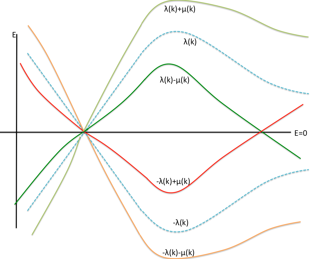
Refer to caption
Figure 14. Spectrum of γ\gamma-quadratic Hamiltonians. If μ=0\mu=0, the spectrum degenerates to the dotted blue lines, which are each 2-fold degenerate.

When μ\mu is zero, the four-band spectrum becomes a pair of doubly-degenerate bands, and these degenerate pairs cross exactly at the points where λ=0\lambda=0, much like the spectrum of the Dirac-type Hamiltonians which are linear in γ\gamma. We are interested in such “bilinear Hamiltonians”, and they are precisely the pure tensor ones H𝒂,𝒃(k)=i2[𝒂(k)𝜸,𝒃(k)𝜸)]=iI(𝒂(k)𝒃(k))IγIH_{\bm{{a}},\bm{{b}}}(k)=\frac{\text{i}}{2}[\bm{{a}}(k)\cdot\bm{{\gamma}},\bm{{b}}(k)\cdot\bm{{\gamma}})]=\text{i}\sum_{I}(\bm{{a}}(k)\wedge\bm{{b}}(k))_{I}\gamma_{I}, specified by a single pair of vector fields (𝒂𝒃)(\bm{{a}}\wedge\bm{{b}}), with spec(H𝒂,𝒃(k))=±|𝒂𝒃|(k)=±λ(k)\text{spec}(H_{\bm{{a}},\bm{{b}}}(k))=\pm|\bm{{a}}\wedge\bm{{b}}|(k)=\pm\lambda(k).

We will assume that the singularities (points where 𝒂𝒃\bm{{a}}\wedge\bm{{b}} vanishes) form a finite set of isolated points WW. In other words, (𝒂,𝒃)(\bm{{a}},\bm{{b}}) defines a tangent 2-field over TWT\setminus W. At a singularity wWw\in W, there may be topological obstructions to extending (𝒂,𝒃)(\bm{{a}},\bm{{b}}) across ww, in which case, we cannot open up a gap at the four-band crossing at ww by simply deforming λ\lambda into a strictly positive function. Despite the spectrum resembling that of a (linear) Dirac-type Hamiltonian, this type of four-band crossing can be topologically protected by a very different and much more subtle mechanism, see Section 5.3.

Remark 5.3.

We may also consider bilinear Hamiltonians H𝒂,𝒃H_{\bm{{a}},\bm{{b}}} specified by a pair of vector fields (𝒂,𝒃)(\bm{{a}},\bm{{b}}) over a dd-manifold with d5d\neq 5. However, it is no longer the case that a 𝖢\mathsf{C}-symmetry singles out such Hamiltonians, and one needs to motivate such model Hamiltonians in a different way. They may nevertheless be studied as a toy model.

5.3. Atiyah–Thomas 2{\mathbb{Z}}_{2}-invariant

A detailed study of tangent 2-fields with finite singularities was carried out in [63, 64, 2, 30], where analogues of the Poincaré–Hopf theorem for vector fields were obtained. For this, we need the notion of the local index at a singularity wWw\in W of a tangent 2-field (𝒂,𝒃)(\bm{{a}},\bm{{b}}) on TWT\setminus W. Let Sw4S_{w}^{4} be a small oriented 4-sphere surrounding wWw\in W, then (𝒂,𝒃)(\bm{{a}},\bm{{b}}) gives a map Sw4W5,2S_{w}^{4}\rightarrow W_{5,2} to the non-compact Stiefel manifold W5,2=GL(5,)/GL(3,)W_{5,2}=\text{GL}(5,{\mathbb{R}})/\text{GL}(3,{\mathbb{R}}) of 2-frames in 5{\mathbb{R}}^{5}. There is a homotopy equivalence between W5,2W_{5,2} and the (compact) Stiefel manifold 𝒱5,2=SO(5)/SO(3)\mathcal{V}_{5,2}=\text{SO}(5)/\text{SO}(3) of orthonormal 2-frames in 5{\mathbb{R}}^{5}. The local index of (𝐚,𝐛)(\bm{{a}},\bm{{b}}) at ww is defined to be the homotopy class of (𝒂,𝒃)|Sw4(\bm{{a}},\bm{{b}})|_{S_{w}^{4}} in π4(W5,2)π4(𝒱5,2)2\pi_{4}(W_{5,2})\cong\pi_{4}(\mathcal{V}_{5,2})\cong{\mathbb{Z}}_{2}, and is the local obstruction to deforming (𝒂,𝒃)(\bm{{a}},\bm{{b}}) to remove the singularity at ww.

Recall from the previous subsection the construction of a bilinear Dirac Hamiltonian H𝒂,𝒃H_{\bm{{a}},\bm{{b}}} from a tangent 2-field (𝒂,𝒃)(\bm{{a}},\bm{{b}}) over TT with finite singularities WW, and that four-band crossings occur precisely at WW. The local index at ww of (𝒂,𝒃)(\bm{{a}},\bm{{b}}) has the physical interpretation as a 2{\mathbb{Z}}_{2} local topological charge protecting the band crossing wWw\in W.

To understand π4(𝒱5,2)2\pi_{4}(\mathcal{V}_{5,2})\cong{\mathbb{Z}}_{2} better, recall the fibration

S3=𝒱4,1𝒱5,2𝒱5,1=S4,S^{3}=\mathcal{V}_{4,1}\rightarrow\mathcal{V}_{5,2}\rightarrow\mathcal{V}_{5,1}=S^{4},

where the S4S^{4} base parametrises the choice of a first normalised vector 𝒂^\hat{\bm{{a}}}, and the fiber parametrises (locally) the choice of 𝒃^\hat{\bm{{b}}} orthonormal to 𝒂^\hat{\bm{{a}}}. From the homotopy exact sequence,

π4(S3)=2π4(𝒱5,2)=2π4(S4)=π3(S3)=\ldots\rightarrow\pi_{4}(S^{3})={\mathbb{Z}}_{2}\rightarrow\pi_{4}(\mathcal{V}_{5,2})={\mathbb{Z}}_{2}\rightarrow\pi_{4}(S^{4})={\mathbb{Z}}\rightarrow\pi_{3}(S^{3})={\mathbb{Z}}\rightarrow\ldots

we see that π4(𝒱5,2)=2\pi_{4}(\mathcal{V}_{5,2})={\mathbb{Z}}_{2} comes from the inclusion of the fiber S3=𝒱4,1S^{3}=\mathcal{V}_{4,1} which has the famous π4(S3)=π4(SU(2))=2\pi_{4}(S^{3})=\pi_{4}(\text{SU}(2))={\mathbb{Z}}_{2}.

Thus, we can construct an explicit example of a 2{\mathbb{Z}}_{2}-protected four-band crossing as follows. Choose some local Euclidean coordinates kk for a neighbourhood 𝒪\mathcal{O} of ww centred at 0, and a trivialization e1,,e5e_{1},\ldots,e_{5} of the tangent bundle above 𝒪\mathcal{O}. Take 𝒂^=e1\hat{\bm{{a}}}=e_{1}, and for kSw4k\in S_{w}^{4}, we choose 𝒃^\hat{\bm{{b}}} orthonormal to 𝒂^\hat{\bm{{a}}} by letting k𝒃^(k)S4k\mapsto\hat{\bm{{b}}}(k)\in S^{4} be given by a generator of π4(𝒱4,1)=π4(S3)\pi_{4}(\mathcal{V}_{4,1})=\pi_{4}(S^{3}). Extend to orthogonal vectors 𝒂,𝒃\bm{{a}},\bm{{b}} to all of 𝒪\mathcal{O} by scaling by |k||k|. Thus H𝒂,𝒃(k)=i|k|I(𝒂^𝒃^(k))IγIH_{\bm{{a}},\bm{{b}}}(k)=\text{i}|k|\sum_{I}(\hat{\bm{{a}}}\wedge\hat{\bm{{b}}}(k))_{I}\gamma_{I} on 𝒪{w}\mathcal{O}\setminus\{w\} and H𝒂,𝒃(w)=0H_{\bm{{a}},\bm{{b}}}(w)=0. Then ww is a four-band crossing with non-trivial 2{\mathbb{Z}}_{2}-charge.

Remark 5.4.

By taking 𝒂𝒃|𝒂𝒃|\frac{\bm{{a}}\wedge\bm{{b}}}{|\bm{{a}}\wedge\bm{{b}}|} we obtain a 2-plane field88 8 2-plane fields are also called oriented 22-distributions, see [30] for a guide to kk-distributions on manifolds. defining for each kTWk\in T\setminus W a point in the oriented Grassmannian 𝒢5,2+\mathcal{G}^{+}_{5,2} of 2-planes in 5{\mathbb{R}}^{5}. For a 2-plane field over TWT\setminus W, there is similarly a map Sw4𝒢5,2+S_{w}^{4}\rightarrow\mathcal{G}^{+}_{5,2}, and a local index can be defined at wWw\in W. Note that 𝒢5,2+=𝒱5,2/SO(2)\mathcal{G}^{+}_{5,2}=\mathcal{V}_{5,2}/\text{SO}(2), and at the level of π4\pi_{4} the exact sequence

0=π5(SO(2))π4(𝒱5,2)π4(𝒢5,2+)0=π4(SO(2))\ldots\rightarrow 0=\pi_{5}(\text{SO}(2))\rightarrow\pi_{4}(\mathcal{V}_{5,2})\xrightarrow{\cong}\pi_{4}(\mathcal{G}^{+}_{5,2})\rightarrow 0=\pi_{4}(\text{SO}(2))\rightarrow\ldots

says that the index is in π4(𝒱5,2)π4(𝒢5,2+)2\pi_{4}(\mathcal{V}_{5,2})\cong\pi_{4}(\mathcal{G}^{+}_{5,2})\cong{\mathbb{Z}}_{2}. Although we can consider bilinear Hamiltonians specified by a field of oriented area elements, i.e. a 2-plane field along with areas (magnitudes), which will also have 2{\mathbb{Z}}_{2} local indices, we only consider those specified by a tangent 2-field (with finite singularities) in this paper.

For tangent 2-fields in d3d\geq 3-dimensions, the local topological index at a point singularity is defined similarly, as an element of πd1(𝒱d,2)\pi_{d-1}(\mathcal{V}_{d,2}). These homotopy groups are known to be 2{\mathbb{Z}}_{2} when dd is odd and 2{\mathbb{Z}}\oplus{\mathbb{Z}}_{2} when dd is even [49]. Unlike the case of vector fields, the global constraint for these indices depends on dd (mod 4) [63, 64, 1, 2] and in the following subsection, we will restrict to d=1d=1 (mod 4) .

5.4. Kervaire semicharacteristic, Kervaire chains and 2{\mathbb{Z}}_{2}-Fermi arcs

For this section, we assume that TT is a compact oriented dd-manifold TT with d=1d=1 (mod 4) and d5d\geq 5. Most of the constructions of Section 3 can be carried out for 2{\mathbb{Z}}_{2} coefficients, and there is also a generalisation of the Poincaré–Hopf theorem for tangent 2-fields and 2-plane fields with finite singularities [63, 64, 1, 2]. This suggests that Hamiltonians parametrised by a tangent 2-field, such as the 5D 2{\mathbb{Z}}_{2}-Dirac semimetals introduced in Section 5.2, can have topologically protected crossings which are furthermore constrained by the global Atiyah–Dupont condition. If κ(T)=0\kappa(T)=0, we expect there to be 2{\mathbb{Z}}_{2}-charge cancellation and also a notion of 2{\mathbb{Z}}_{2}-Fermi arcs.

Let us simplify notation and write 𝒫\mathcal{P} for the tangent 2-field (𝒂,𝒃)(\bm{{a}},\bm{{b}}) over TWT\setminus W, and Indw(𝒫)\text{Ind}_{w}(\mathcal{P}) for its local 2{\mathbb{Z}}_{2} charge at wWw\in W, which is assumed to be a finite set as before. The sum Ind(𝒫)=wWIndw(𝒫)\text{Ind}(\mathcal{P})=\sum_{w\in W}\text{Ind}_{w}(\mathcal{P}) is a global obstruction to deforming 𝒫\mathcal{P} to a tangent 2-field on all of TT. In [2], Atiyah–Dupont proved that Ind(𝒫)\text{Ind}(\mathcal{P}) is equal to the real Kervaire semicharacteristic κ(T)\kappa(T), defined as

κ(T)=qevendimHq(T,)mod 2.\kappa(T)=\sum_{q\,\text{even}}\text{dim}_{\mathbb{R}}\,H^{q}(T,{\mathbb{R}})\;\;\text{mod }2.

Thus Ind(𝒫)=κ(T)\text{Ind}(\mathcal{P})=\kappa(T) for any 𝒫\mathcal{P}. It is known that the manifold TT admits tangent 2-fields 𝒫\mathcal{P} with finite singularity set WW if and only if the Stiefel–Whitney class wd1(T)w_{d-1}(T) vanishes, ([64]), which holds for instance when T=𝕋dT={\mathbb{T}}^{d}, in which case the Kervaire semicharacteristic vanishes, κ(𝕋d)=0\kappa({\mathbb{T}}^{d})=0.

Remark 5.5.

Although we have assumed the bilinear Hamiltonians to be specified by tangent 2-fields, we could also work more generally with 2-fields for other vector bundles using a generalisation of the Atiyah–Dupont theory in [61].

Definition 5.1.

Let TT be a compact oriented dd-manifold TT with d=1d=1 (mod 4) and κ(T)=0\kappa(T)=0. For a 0-chain 𝒲C0(T,2)\mathcal{W}\in C_{0}(T,{\mathbb{Z}}_{2}) defined on WW and with total weight zero, a Kervaire chain for 𝒲\mathcal{W} is a 1-chain lC1(T,2)l\in C_{1}(T,{\mathbb{Z}}_{2}) such that l=𝒲\partial l=\mathcal{W}, thus [l]H1(T,W,2)[l]\in H_{1}(T,W,{\mathbb{Z}}_{2}). We write 𝔎𝔢𝔯𝔳(T,𝒲)\mathfrak{Kerv}(T,\mathcal{W}) for the subset of homology classes of Kervaire chains for 𝒲\mathcal{W}.

The 2{\mathbb{Z}}_{2}-versions of the semimetal MV sequence and the dual homology sequence are

    0          Hd1(T,2)    PD                Hd1(TW,2)    PD          β         Hd1(SW,2)    PD          Σ         Hd(T,2)    PD                0   0          H1(T,2)          H1(T,W,2)             H0(W,2)    Σ         H0(T,2)          0    .\small\lx@xy@svg{\hbox{\raise 2.31248pt\hbox{\kern 5.31248pt\hbox{\ignorespaces\ignorespaces\ignorespaces\hbox{\vtop{\halign{\entry@#!@&&\entry@@#!@\cr&&&&&\cr&&&&&\crcr}}}\ignorespaces{\hbox{\kern-5.31248pt\raise 0.0pt\hbox{\hbox{\kern 0.0pt\raise 0.0pt\hbox{\hbox{\kern 3.0pt\raise-2.31248pt\hbox{$\textstyle{0\ignorespaces\ignorespaces\ignorespaces\ignorespaces}$}}}}}}}\ignorespaces\ignorespaces\ignorespaces\ignorespaces{}{\hbox{\lx@xy@droprule}}\ignorespaces{\hbox{\kern 29.31248pt\raise 0.0pt\hbox{\hbox{\kern 0.0pt\raise 0.0pt\hbox{\lx@xy@tip{1}\lx@xy@tip{-1}}}}}}{\hbox{\lx@xy@droprule}}{\hbox{\lx@xy@droprule}}{\hbox{\kern 29.31248pt\raise 0.0pt\hbox{\hbox{\kern 0.0pt\raise 0.0pt\hbox{\hbox{\kern 3.0pt\raise-2.31248pt\hbox{$\textstyle{H^{d-1}(T,{\mathbb{Z}}_{2})\ignorespaces\ignorespaces\ignorespaces\ignorespaces\ignorespaces\ignorespaces\ignorespaces\ignorespaces}$}}}}}}}\ignorespaces\ignorespaces\ignorespaces\ignorespaces{}{\hbox{\lx@xy@droprule}}\ignorespaces\ignorespaces\ignorespaces{\hbox{\kern 38.0481pt\raise-16.08083pt\hbox{{}\hbox{\kern 0.0pt\raise 0.0pt\hbox{\hbox{\kern 3.0pt\hbox{\hbox{\kern 0.0pt\raise-2.1525pt\hbox{$\scriptstyle{\text{PD}}$}}}\kern 3.0pt}}}}}}\ignorespaces{\hbox{\kern 54.97379pt\raise-24.72414pt\hbox{\hbox{\kern 0.0pt\raise 0.0pt\hbox{\lx@xy@tip{1}\lx@xy@tip{-1}}}}}}{\hbox{\lx@xy@droprule}}{\hbox{\lx@xy@droprule}}\ignorespaces\ignorespaces\ignorespaces\ignorespaces{}{\hbox{\lx@xy@droprule}}\ignorespaces{\hbox{\kern 104.63509pt\raise 0.0pt\hbox{\hbox{\kern 0.0pt\raise 0.0pt\hbox{\lx@xy@tip{1}\lx@xy@tip{-1}}}}}}{\hbox{\lx@xy@droprule}}{\hbox{\lx@xy@droprule}}{\hbox{\kern 104.63509pt\raise 0.0pt\hbox{\hbox{\kern 0.0pt\raise 0.0pt\hbox{\hbox{\kern 3.0pt\raise-2.31248pt\hbox{$\textstyle{H^{d-1}(T\setminus W,{\mathbb{Z}}_{2})\ignorespaces\ignorespaces\ignorespaces\ignorespaces\ignorespaces\ignorespaces\ignorespaces\ignorespaces}$}}}}}}}\ignorespaces\ignorespaces\ignorespaces\ignorespaces{}{\hbox{\lx@xy@droprule}}\ignorespaces\ignorespaces\ignorespaces{\hbox{\kern 123.51924pt\raise-16.08083pt\hbox{{}\hbox{\kern 0.0pt\raise 0.0pt\hbox{\hbox{\kern 3.0pt\hbox{\hbox{\kern 0.0pt\raise-2.1525pt\hbox{$\scriptstyle{\text{PD}}$}}}\kern 3.0pt}}}}}}\ignorespaces{\hbox{\kern 140.44493pt\raise-24.72414pt\hbox{\hbox{\kern 0.0pt\raise 0.0pt\hbox{\lx@xy@tip{1}\lx@xy@tip{-1}}}}}}{\hbox{\lx@xy@droprule}}{\hbox{\lx@xy@droprule}}\ignorespaces\ignorespaces\ignorespaces\ignorespaces{}{\hbox{\lx@xy@droprule}}\ignorespaces\ignorespaces\ignorespaces{\hbox{\kern 180.17348pt\raise 5.8pt\hbox{{}\hbox{\kern 0.0pt\raise 0.0pt\hbox{\hbox{\kern 3.0pt\hbox{\hbox{\kern 0.0pt\raise-1.575pt\hbox{$\scriptstyle{\beta}$}}}\kern 3.0pt}}}}}}\ignorespaces{\hbox{\kern 200.25478pt\raise 0.0pt\hbox{\hbox{\kern 0.0pt\raise 0.0pt\hbox{\lx@xy@tip{1}\lx@xy@tip{-1}}}}}}{\hbox{\lx@xy@droprule}}{\hbox{\lx@xy@droprule}}{\hbox{\kern 200.25478pt\raise 0.0pt\hbox{\hbox{\kern 0.0pt\raise 0.0pt\hbox{\hbox{\kern 3.0pt\raise-2.31248pt\hbox{$\textstyle{H^{d-1}(S_{W},{\mathbb{Z}}_{2})\ignorespaces\ignorespaces\ignorespaces\ignorespaces\ignorespaces\ignorespaces\ignorespaces\ignorespaces}$}}}}}}}\ignorespaces\ignorespaces\ignorespaces\ignorespaces{}{\hbox{\lx@xy@droprule}}\ignorespaces\ignorespaces\ignorespaces{\hbox{\kern 213.37392pt\raise-16.08083pt\hbox{{}\hbox{\kern 0.0pt\raise 0.0pt\hbox{\hbox{\kern 3.0pt\hbox{\hbox{\kern 0.0pt\raise-2.1525pt\hbox{$\scriptstyle{\text{PD}}$}}}\kern 3.0pt}}}}}}\ignorespaces{\hbox{\kern 230.2996pt\raise-24.72414pt\hbox{\hbox{\kern 0.0pt\raise 0.0pt\hbox{\lx@xy@tip{1}\lx@xy@tip{-1}}}}}}{\hbox{\lx@xy@droprule}}{\hbox{\lx@xy@droprule}}\ignorespaces\ignorespaces\ignorespaces\ignorespaces{}{\hbox{\lx@xy@droprule}}\ignorespaces\ignorespaces\ignorespaces{\hbox{\kern 262.7923pt\raise 5.1525pt\hbox{{}\hbox{\kern 0.0pt\raise 0.0pt\hbox{\hbox{\kern 3.0pt\hbox{\hbox{\kern 0.0pt\raise-2.1525pt\hbox{$\scriptstyle{\Sigma}$}}}\kern 3.0pt}}}}}}\ignorespaces{\hbox{\kern 284.34444pt\raise 0.0pt\hbox{\hbox{\kern 0.0pt\raise 0.0pt\hbox{\lx@xy@tip{1}\lx@xy@tip{-1}}}}}}{\hbox{\lx@xy@droprule}}{\hbox{\lx@xy@droprule}}{\hbox{\kern 284.34444pt\raise 0.0pt\hbox{\hbox{\kern 0.0pt\raise 0.0pt\hbox{\hbox{\kern 3.0pt\raise-2.31248pt\hbox{$\textstyle{H^{d}(T,{\mathbb{Z}}_{2})\ignorespaces\ignorespaces\ignorespaces\ignorespaces\ignorespaces\ignorespaces\ignorespaces\ignorespaces}$}}}}}}}\ignorespaces\ignorespaces\ignorespaces\ignorespaces{}{\hbox{\lx@xy@droprule}}\ignorespaces\ignorespaces\ignorespaces{\hbox{\kern 289.84259pt\raise-16.08083pt\hbox{{}\hbox{\kern 0.0pt\raise 0.0pt\hbox{\hbox{\kern 3.0pt\hbox{\hbox{\kern 0.0pt\raise-2.1525pt\hbox{$\scriptstyle{\text{PD}}$}}}\kern 3.0pt}}}}}}\ignorespaces{\hbox{\kern 306.76828pt\raise-24.72414pt\hbox{\hbox{\kern 0.0pt\raise 0.0pt\hbox{\lx@xy@tip{1}\lx@xy@tip{-1}}}}}}{\hbox{\lx@xy@droprule}}{\hbox{\lx@xy@droprule}}\ignorespaces\ignorespaces\ignorespaces\ignorespaces{}{\hbox{\lx@xy@droprule}}\ignorespaces{\hbox{\kern 353.19212pt\raise 0.0pt\hbox{\hbox{\kern 0.0pt\raise 0.0pt\hbox{\lx@xy@tip{1}\lx@xy@tip{-1}}}}}}{\hbox{\lx@xy@droprule}}{\hbox{\lx@xy@droprule}}{\hbox{\kern 353.19212pt\raise 0.0pt\hbox{\hbox{\kern 0.0pt\raise 0.0pt\hbox{\hbox{\kern 3.0pt\raise-2.31248pt\hbox{$\textstyle{0}$}}}}}}}{\hbox{\kern-5.31248pt\raise-32.16165pt\hbox{\hbox{\kern 0.0pt\raise 0.0pt\hbox{\hbox{\kern 3.0pt\raise-2.31248pt\hbox{$\textstyle{0\ignorespaces\ignorespaces\ignorespaces\ignorespaces}$}}}}}}}\ignorespaces\ignorespaces\ignorespaces\ignorespaces{}{\hbox{\lx@xy@droprule}}\ignorespaces{\hbox{\kern 32.64876pt\raise-32.16165pt\hbox{\hbox{\kern 0.0pt\raise 0.0pt\hbox{\lx@xy@tip{1}\lx@xy@tip{-1}}}}}}{\hbox{\lx@xy@droprule}}{\hbox{\lx@xy@droprule}}{\hbox{\kern 32.64876pt\raise-32.16165pt\hbox{\hbox{\kern 0.0pt\raise 0.0pt\hbox{\hbox{\kern 3.0pt\raise-2.31248pt\hbox{$\textstyle{H_{1}(T,{\mathbb{Z}}_{2})\ignorespaces\ignorespaces\ignorespaces\ignorespaces}$}}}}}}}\ignorespaces\ignorespaces\ignorespaces\ignorespaces{}{\hbox{\lx@xy@droprule}}\ignorespaces{\hbox{\kern 111.8255pt\raise-32.16165pt\hbox{\hbox{\kern 0.0pt\raise 0.0pt\hbox{\lx@xy@tip{1}\lx@xy@tip{-1}}}}}}{\hbox{\lx@xy@droprule}}{\hbox{\lx@xy@droprule}}{\hbox{\kern 111.8255pt\raise-32.16165pt\hbox{\hbox{\kern 0.0pt\raise 0.0pt\hbox{\hbox{\kern 3.0pt\raise-2.31248pt\hbox{$\textstyle{H_{1}(T,W,{\mathbb{Z}}_{2})\ignorespaces\ignorespaces\ignorespaces\ignorespaces}$}}}}}}}\ignorespaces\ignorespaces\ignorespaces\ignorespaces{}{\hbox{\lx@xy@droprule}}\ignorespaces\ignorespaces\ignorespaces{\hbox{\kern 180.29742pt\raise-26.97415pt\hbox{{}\hbox{\kern 0.0pt\raise 0.0pt\hbox{\hbox{\kern 3.0pt\hbox{\hbox{\kern 0.0pt\raise-2.1875pt\hbox{$\scriptstyle{\partial}$}}}\kern 3.0pt}}}}}}\ignorespaces{\hbox{\kern 206.8192pt\raise-32.16165pt\hbox{\hbox{\kern 0.0pt\raise 0.0pt\hbox{\lx@xy@tip{1}\lx@xy@tip{-1}}}}}}{\hbox{\lx@xy@droprule}}{\hbox{\lx@xy@droprule}}{\hbox{\kern 206.8192pt\raise-32.16165pt\hbox{\hbox{\kern 0.0pt\raise 0.0pt\hbox{\hbox{\kern 3.0pt\raise-2.31248pt\hbox{$\textstyle{H_{0}(W,{\mathbb{Z}}_{2})\ignorespaces\ignorespaces\ignorespaces\ignorespaces}$}}}}}}}\ignorespaces\ignorespaces\ignorespaces\ignorespaces{}{\hbox{\lx@xy@droprule}}\ignorespaces\ignorespaces\ignorespaces{\hbox{\kern 262.7923pt\raise-27.00916pt\hbox{{}\hbox{\kern 0.0pt\raise 0.0pt\hbox{\hbox{\kern 3.0pt\hbox{\hbox{\kern 0.0pt\raise-2.1525pt\hbox{$\scriptstyle{\Sigma}$}}}\kern 3.0pt}}}}}}\ignorespaces{\hbox{\kern 284.44325pt\raise-32.16165pt\hbox{\hbox{\kern 0.0pt\raise 0.0pt\hbox{\lx@xy@tip{1}\lx@xy@tip{-1}}}}}}{\hbox{\lx@xy@droprule}}{\hbox{\lx@xy@droprule}}{\hbox{\kern 284.44325pt\raise-32.16165pt\hbox{\hbox{\kern 0.0pt\raise 0.0pt\hbox{\hbox{\kern 3.0pt\raise-2.31248pt\hbox{$\textstyle{H_{0}(T,{\mathbb{Z}}_{2})\ignorespaces\ignorespaces\ignorespaces\ignorespaces}$}}}}}}}\ignorespaces\ignorespaces\ignorespaces\ignorespaces{}{\hbox{\lx@xy@droprule}}\ignorespaces{\hbox{\kern 353.19212pt\raise-32.16165pt\hbox{\hbox{\kern 0.0pt\raise 0.0pt\hbox{\lx@xy@tip{1}\lx@xy@tip{-1}}}}}}{\hbox{\lx@xy@droprule}}{\hbox{\lx@xy@droprule}}{\hbox{\kern 353.19212pt\raise-32.16165pt\hbox{\hbox{\kern 0.0pt\raise 0.0pt\hbox{\hbox{\kern 3.0pt\raise-2.31248pt\hbox{$\textstyle{0}$}}}}}}}\ignorespaces}}}}\ignorespaces.\normalsize

As before, we define 𝔠𝔬𝔎𝔢𝔯𝔳(T,𝒲)Hd1(TW,2)\mathfrak{coKerv}(T,\mathcal{W})\subset H^{d-1}(T\setminus W,{\mathbb{Z}}_{2}) to be the Poincaré dual image of 𝔎𝔢𝔯𝔳(T,𝒲)\mathfrak{Kerv}(T,\mathcal{W}). We will then explain how a tangent 2-field with finite singularity set WW has a topological invariant in 𝔠𝔬𝔎𝔢𝔯𝔳(T,𝒲)\mathfrak{coKerv}(T,\mathcal{W}) and therefore a Kervaire chain representation.

Definition 5.2.

Let TT be a compact oriented dd-manifold TT with d=1d=1 (mod 4) and κ(T)=0\kappa(T)=0, and 𝒮\mathcal{S} be the sphere bundle for its tangent bundle. A Kervaire structure for TT is a class in Hd1(𝒮,2)H^{d-1}(\mathcal{S},{\mathbb{Z}}_{2}) whose restriction to each fibre 𝒮k,kT\mathcal{S}_{k},k\in T generates Hd1(Sd1,2)H^{d-1}(S^{d-1},{\mathbb{Z}}_{2}). Define 𝔠𝔬𝔎𝔢𝔯𝔳~(T)\widetilde{\mathfrak{coKerv}}(T) to be the set of Kervaire structures for TT.

From the Gysin sequence (3.1) with 2{\mathbb{Z}}_{2}-coefficients, we see that Hd1(T,2)H^{d-1}(T,{\mathbb{Z}}_{2}) acts on 𝔠𝔬𝔎𝔢𝔯𝔳~(T)\widetilde{\mathfrak{coKerv}}(T) freely and transitively by pullback and addition. Let 𝒱d,2T{\mathscr{V}}_{d,2}T be the bundle of Stiefel manifolds 𝒱d,2\mathcal{V}_{d,2} associated to the orthonormal frame bundle of TT (endowed with some Riemannian metric). Corresponding to the fibration Sd2=𝒱d1,1𝒱d,2𝒱d,1=Sd1S^{d-2}=\mathcal{V}_{d-1,1}\rightarrow\mathcal{V}_{d,2}\rightarrow\mathcal{V}_{d,1}=S^{d-1}, there is a fibration

Sd2𝒱d,2𝜌𝒮.S^{d-2}\rightarrow{\mathscr{V}}_{d,2}\overset{\rho}{\longrightarrow}\mathcal{S}.

A (non-singular) tangent 2-field 𝒫\mathcal{P} on TT gives rise to a Kervaire structure as follows. Let 𝒫^\widehat{\mathcal{P}} denote the section of 𝒱d,2{\mathscr{V}}_{d,2} determined by 𝒫\mathcal{P}, which is a dd-cycle on 𝒱d,2{\mathscr{V}}_{d,2}. The Poincaré dual is a (2d3)(2d-3)-cocycle on 𝒱d,2{\mathscr{V}}_{d,2}, and pushforward under ρ\rho gives a (d1)(d-1)-cocycle in 𝒮\mathcal{S}. Furthermore, the construction of the cocycle is such that its restriction to 𝒮k\mathcal{S}_{k} generates Hd1(Sd1,2)H^{d-1}(S^{d-1},{\mathbb{Z}}_{2}) for each kTk\in T.

Now consider tangent 2-fields on TT with finite singularities WW. As in Section 3.4, we can define a local charge operator

β~:Hd1(𝒮|TW,2)Hd1(SW,2)PDH1(W,2).\tilde{\beta}:H^{d-1}(\mathcal{S}|_{T\setminus W},{\mathbb{Z}}_{2})\rightarrow H^{d-1}(S_{W},{\mathbb{Z}}_{2})\overset{\text{PD}}{\longleftrightarrow}H_{1}(W,{\mathbb{Z}}_{2}).

Then for each 0-chain 𝒲\mathcal{W} with total charge zero, we define 𝔠𝔬𝔎𝔢𝔯𝔳~(T,𝒲)\widetilde{\mathfrak{coKerv}}(T,\mathcal{W}) to be the subset of Hd1(𝒮TW,2)H^{d-1}(\mathcal{S}_{T\setminus W},{\mathbb{Z}}_{2}) whose restriction to each fibre over kTWk\in T\setminus W generates Hd1(Sd1,2)H^{d-1}(S^{d-1},{\mathbb{Z}}_{2}), and whose local charges is PD(𝒲)\text{PD}(\mathcal{W}). Each 𝔠𝔬𝔎𝔢𝔯𝔳~(T,𝒲)\widetilde{\mathfrak{coKerv}}(T,\mathcal{W}) is an affine space for Hd1(T,2)H^{d-1}(T,{\mathbb{Z}}_{2}). Suppose 𝒫\mathcal{P} is a tangent 2-field on TWT\setminus W with local charge 0-chain 𝒲\mathcal{W}, then it determines a dd-cycle in 𝒱d,2|TDW{\mathscr{V}}_{d,2}|_{T\setminus D_{W}} relative to the boundary 𝒱d,2|SW{\mathscr{V}}_{d,2}|_{S_{W}}, which Poincaré dualises to a (2d3)(2d-3)-cocycle on 𝒱d,2|TDW{\mathscr{V}}_{d,2}|_{T\setminus D_{W}}. Pushforward under ρ\rho gives a (d1)(d-1)-cocycle on 𝒮|TDW\mathcal{S}|_{T\setminus D_{W}} representing a class in 𝔠𝔬𝔎𝔢𝔯𝔳~(T,𝒲)\widetilde{\mathfrak{coKerv}}(T,\mathcal{W}). Fix a reference non-singular vector field 𝒉ref\bm{{h}}_{\text{ref}}, then 𝒉ref\bm{{h}}_{\text{ref}}^{*} identifies 𝔠𝔬𝔎𝔢𝔯𝔳~(T,𝒲)\widetilde{\mathfrak{coKerv}}(T,\mathcal{W}) with 𝔠𝔬𝔎𝔢𝔯𝔳(T,𝒲)\mathfrak{coKerv}(T,\mathcal{W}).

The following diagram summarises the various affines spaces for H1(T,2)Hd1(T,2)H_{1}(T,{\mathbb{Z}}_{2})\cong H^{d-1}(T,{\mathbb{Z}}_{2}):

    H1(T,2)                 𝔎𝔢𝔯𝔳(T,𝒲)                 H1(T,W,2)   Hd1(T,2)                        𝔠𝔬𝔎𝔢𝔯𝔳(T,𝒲)                        Hd1(TW,2)   Hd1(𝒮,2)   𝔠𝔬𝔎𝔢𝔯𝔳~(T)                 𝔠𝔬𝔎𝔢𝔯𝔳~(T,𝒲)                 Hd1(𝒮|TW,2)    .\lx@xy@svg{\hbox{\raise 2.5pt\hbox{\kern 31.86617pt\hbox{\ignorespaces\ignorespaces\ignorespaces\hbox{\vtop{\halign{\entry@#!@&&\entry@@#!@\cr&&&\cr&&&\cr&&&\crcr}}}\ignorespaces{\hbox{\kern-3.0pt\raise 0.0pt\hbox{\hbox{\kern 0.0pt\raise 0.0pt\hbox{\hbox{\kern 3.0pt\raise-2.5pt\hbox{$\textstyle{}$}}}}}}}{\hbox{\kern 59.29483pt\raise 0.0pt\hbox{\hbox{\kern 0.0pt\raise 0.0pt\hbox{\hbox{\kern 3.0pt\raise-2.5pt\hbox{$\textstyle{H_{1}(T,{\mathbb{Z}}_{2})\ignorespaces\ignorespaces\ignorespaces\ignorespaces\ignorespaces\ignorespaces\ignorespaces\ignorespaces}$}}}}}}}\ignorespaces\ignorespaces\ignorespaces\ignorespaces{}{\hbox{\lx@xy@droprule}}\ignorespaces{\hbox{\kern 138.88673pt\raise 0.0pt\hbox{\hbox{\kern 0.0pt\raise 0.0pt\hbox{\lx@xy@tip{1}\lx@xy@tip{-1}}}}}}{\hbox{\lx@xy@droprule}}{\hbox{\lx@xy@droprule}}\ignorespaces\ignorespaces\ignorespaces\ignorespaces{}{\hbox{\lx@xy@droprule}}\ignorespaces{\hbox{\kern 83.01534pt\raise-23.50499pt\hbox{\hbox{\kern 0.0pt\raise 0.0pt\hbox{\lx@xy@tip{1}\lx@xy@tip{-1}}}}}}{\hbox{\lx@xy@droprule}}{\hbox{\lx@xy@droprule}}{\hbox{\kern 138.88673pt\raise 0.0pt\hbox{\hbox{\kern 0.0pt\raise 0.0pt\hbox{\hbox{\kern 3.0pt\raise-2.5pt\hbox{$\textstyle{\mathfrak{Kerv}(T,\mathcal{W})\ignorespaces\ignorespaces\ignorespaces\ignorespaces\ignorespaces\ignorespaces\ignorespaces\ignorespaces}$}}}}}}}\ignorespaces\ignorespaces\ignorespaces\ignorespaces{}{\hbox{\lx@xy@droprule}}\ignorespaces{\hbox{\kern 106.73586pt\raise 0.0pt\hbox{\hbox{\kern 0.0pt\raise 0.0pt\hbox{\lx@xy@tip{1}\lx@xy@tip{-1}}}}}}{\hbox{\lx@xy@droprule}}{\hbox{\lx@xy@droprule}}\ignorespaces\ignorespaces\ignorespaces\ignorespaces{}{\hbox{\lx@xy@droprule}}\ignorespaces{\hbox{\kern 166.35033pt\raise-24.49501pt\hbox{\hbox{\kern 0.0pt\raise 0.0pt\hbox{\lx@xy@tip{1}\lx@xy@tip{-1}}}}}}{\hbox{\lx@xy@droprule}}{\hbox{\lx@xy@droprule}}{\hbox{\kern 224.172pt\raise 0.0pt\hbox{\hbox{\kern 0.0pt\raise 0.0pt\hbox{\hbox{\kern 3.0pt\raise-2.5pt\hbox{$\textstyle{\subset\quad\;\;H_{1}(T,W,{\mathbb{Z}}_{2})}$}}}}}}}{\hbox{\kern-3.0pt\raise-32.49501pt\hbox{\hbox{\kern 0.0pt\raise 0.0pt\hbox{\hbox{\kern 3.0pt\raise-2.5pt\hbox{$\textstyle{}$}}}}}}}{\hbox{\kern 55.86617pt\raise-32.49501pt\hbox{\hbox{\kern 0.0pt\raise 0.0pt\hbox{\hbox{\kern 3.0pt\raise-2.5pt\hbox{$\textstyle{H^{d-1}(T,{\mathbb{Z}}_{2})\ignorespaces\ignorespaces\ignorespaces\ignorespaces\ignorespaces\ignorespaces\ignorespaces\ignorespaces\ignorespaces\ignorespaces\ignorespaces\ignorespaces}$}}}}}}}\ignorespaces\ignorespaces\ignorespaces\ignorespaces{}{\hbox{\lx@xy@droprule}}\ignorespaces{\hbox{\kern 134.1645pt\raise-32.49501pt\hbox{\hbox{\kern 0.0pt\raise 0.0pt\hbox{\lx@xy@tip{1}\lx@xy@tip{-1}}}}}}{\hbox{\lx@xy@droprule}}{\hbox{\lx@xy@droprule}}\ignorespaces\ignorespaces\ignorespaces\ignorespaces{}{\hbox{\lx@xy@droprule}}\ignorespaces{\hbox{\kern 83.01534pt\raise-57.48503pt\hbox{\hbox{\kern 0.0pt\raise 0.0pt\hbox{\lx@xy@tip{1}\lx@xy@tip{-1}}}}}}{\hbox{\lx@xy@droprule}}{\hbox{\lx@xy@droprule}}\ignorespaces\ignorespaces\ignorespaces\ignorespaces{}{\hbox{\lx@xy@droprule}}\ignorespaces{\hbox{\kern 83.01534pt\raise-8.0pt\hbox{\hbox{\kern 0.0pt\raise 0.0pt\hbox{\lx@xy@tip{1}\lx@xy@tip{-1}}}}}}{\hbox{\lx@xy@droprule}}{\hbox{\lx@xy@droprule}}{\hbox{\kern 134.1645pt\raise-32.49501pt\hbox{\hbox{\kern 0.0pt\raise 0.0pt\hbox{\hbox{\kern 3.0pt\raise-2.5pt\hbox{$\textstyle{\mathfrak{coKerv}(T,\mathcal{W})\ignorespaces\ignorespaces\ignorespaces\ignorespaces\ignorespaces\ignorespaces\ignorespaces\ignorespaces\ignorespaces\ignorespaces\ignorespaces\ignorespaces}$}}}}}}}\ignorespaces\ignorespaces\ignorespaces\ignorespaces{}{\hbox{\lx@xy@droprule}}\ignorespaces{\hbox{\kern 110.16452pt\raise-32.49501pt\hbox{\hbox{\kern 0.0pt\raise 0.0pt\hbox{\lx@xy@tip{1}\lx@xy@tip{-1}}}}}}{\hbox{\lx@xy@droprule}}{\hbox{\lx@xy@droprule}}\ignorespaces\ignorespaces\ignorespaces\ignorespaces{}{\hbox{\lx@xy@droprule}}\ignorespaces{\hbox{\kern 166.35033pt\raise-57.48503pt\hbox{\hbox{\kern 0.0pt\raise 0.0pt\hbox{\lx@xy@tip{1}\lx@xy@tip{-1}}}}}}{\hbox{\lx@xy@droprule}}{\hbox{\lx@xy@droprule}}\ignorespaces\ignorespaces\ignorespaces\ignorespaces{}{\hbox{\lx@xy@droprule}}\ignorespaces{\hbox{\kern 166.35033pt\raise-8.0pt\hbox{\hbox{\kern 0.0pt\raise 0.0pt\hbox{\lx@xy@tip{1}\lx@xy@tip{-1}}}}}}{\hbox{\lx@xy@droprule}}{\hbox{\lx@xy@droprule}}{\hbox{\kern 222.96556pt\raise-32.49501pt\hbox{\hbox{\kern 0.0pt\raise 0.0pt\hbox{\hbox{\kern 3.0pt\raise-2.5pt\hbox{$\textstyle{\subset H^{d-1}(T\setminus W,{\mathbb{Z}}_{2})}$}}}}}}}{\hbox{\kern-31.86617pt\raise-65.48503pt\hbox{\hbox{\kern 0.0pt\raise 0.0pt\hbox{\hbox{\kern 3.0pt\raise-2.5pt\hbox{$\textstyle{H^{d-1}(\mathcal{S},{\mathbb{Z}}_{2})\supset}$}}}}}}}{\hbox{\kern 69.73233pt\raise-65.48503pt\hbox{\hbox{\kern 0.0pt\raise 0.0pt\hbox{\hbox{\kern 3.0pt\raise-2.5pt\hbox{$\textstyle{\widetilde{\mathfrak{coKerv}}(T)\ignorespaces\ignorespaces\ignorespaces\ignorespaces\ignorespaces\ignorespaces\ignorespaces\ignorespaces}$}}}}}}}\ignorespaces\ignorespaces\ignorespaces\ignorespaces{}{\hbox{\lx@xy@droprule}}\ignorespaces{\hbox{\kern 146.8173pt\raise-65.48503pt\hbox{\hbox{\kern 0.0pt\raise 0.0pt\hbox{\lx@xy@tip{1}\lx@xy@tip{-1}}}}}}{\hbox{\lx@xy@droprule}}{\hbox{\lx@xy@droprule}}\ignorespaces\ignorespaces\ignorespaces\ignorespaces{}{\hbox{\lx@xy@droprule}}\ignorespaces{\hbox{\kern 83.01534pt\raise-40.49501pt\hbox{\hbox{\kern 0.0pt\raise 0.0pt\hbox{\lx@xy@tip{1}\lx@xy@tip{-1}}}}}}{\hbox{\lx@xy@droprule}}{\hbox{\lx@xy@droprule}}{\hbox{\kern 146.8173pt\raise-65.48503pt\hbox{\hbox{\kern 0.0pt\raise 0.0pt\hbox{\hbox{\kern 3.0pt\raise-2.5pt\hbox{$\textstyle{\widetilde{\mathfrak{coKerv}}(T,\mathcal{W})\ignorespaces\ignorespaces\ignorespaces\ignorespaces\ignorespaces\ignorespaces\ignorespaces\ignorespaces}$}}}}}}}\ignorespaces\ignorespaces\ignorespaces\ignorespaces{}{\hbox{\lx@xy@droprule}}\ignorespaces{\hbox{\kern 96.29836pt\raise-65.48503pt\hbox{\hbox{\kern 0.0pt\raise 0.0pt\hbox{\lx@xy@tip{1}\lx@xy@tip{-1}}}}}}{\hbox{\lx@xy@droprule}}{\hbox{\lx@xy@droprule}}\ignorespaces\ignorespaces\ignorespaces\ignorespaces{}{\hbox{\lx@xy@droprule}}\ignorespaces{\hbox{\kern 166.35033pt\raise-40.49501pt\hbox{\hbox{\kern 0.0pt\raise 0.0pt\hbox{\lx@xy@tip{1}\lx@xy@tip{-1}}}}}}{\hbox{\lx@xy@droprule}}{\hbox{\lx@xy@droprule}}{\hbox{\kern 222.53615pt\raise-65.48503pt\hbox{\hbox{\kern 0.0pt\raise 0.0pt\hbox{\hbox{\kern 3.0pt\raise-2.5pt\hbox{$\textstyle{\subset H^{d-1}(\mathcal{S}|_{T\setminus W},{\mathbb{Z}}_{2})}$}}}}}}}\ignorespaces}}}}\ignorespaces.
Definition 5.3.

Let HH be a bilinear Hamiltonian specified by a tangent 2-field 𝒫\mathcal{P} over a compact oriented 5-manifold TT with κ(T)=0\kappa(T)=0, with finite singularities WW. It has a cohomological topological invariant [ω𝒫]H4(TW,2)[\omega_{\mathcal{P}}]\in H^{4}(T\setminus W,{\mathbb{Z}}_{2}) defined as in the previous paragraph, and its Kervaire chain representation is the Poincaré dual [l𝒫]H1(T,W,2)[l_{\mathcal{P}}]\in H_{1}(T,W,{\mathbb{Z}}_{2}).

2{\mathbb{Z}}_{2}-Fermi arcs

The bulk-boundary correspondence proceeds exactly as before, taking a Kervaire chain for 𝒲\mathcal{W} to a “2{\mathbb{Z}}_{2}-Fermi arc” with topological invariant in H1(T~,W~,2)H_{1}(\widetilde{T},\widetilde{W},{\mathbb{Z}}_{2}). Unlike the usual {\mathbb{Z}}-Fermi arcs, the 2{\mathbb{Z}}_{2}-Fermi arcs cancel in pairs so that there is at most one arc between two projected band crossings, and the arc never fully winds around a 1-cycle in T~\widetilde{T}.

Remark 5.6.

It is known that 𝖳\mathsf{T}-invariant insulators in 2D and 3D, where 𝖳\mathsf{T} now refers to ordinary time-reversal rather than the combination 𝖳𝖯\mathsf{T}\mathsf{P}), are classified by certain 2{\mathbb{Z}}_{2}-valued Fu–Kane–Mele (FKM) invariants [20, 15]. In ongoing work, we are applying the ideas of this paper to understand 𝖳\mathsf{T}-invariant semimetals, which were experimentally realised in [37, 73, 29]. In this setting, the band crossings appear at conjugate-momentum pairs, and the points wi,τ(wi)w_{i},\tau(w_{i}) in each pair have the same integer charge. The relation of these local {\mathbb{Z}} charges to FKM 2{\mathbb{Z}}_{2}-invariants is a subtle generalisation of the relation to weak Chern numbers in the 𝖳\mathsf{T}-broken case. We emphasize that the 2{\mathbb{Z}}_{2} invariants there are mathematically different from the ones due to Atiyah–Dupoint–Thomas and the Kervaire semicharacteristic, and arise under physically different symmetry conditions.

6. Outlook and acknowledgements

The topological semimetal-insulator relationship encoded in the semimetal MV sequence can, in principle, be refined using an MV sequence in differential cohomology [56]. Another refinement comes from additional spatial symmetries. For example, a spatial inversion symmetry 𝖯\mathsf{P} induces an action on the Brillouin torus TT under which WW should be invariant. The same action arises if 𝖳\mathsf{T} rather than 𝖳𝖯\mathsf{T}\mathsf{P} symmetry is present. The vector field 𝒉\bm{{h}} needs to be suitably equivariant, and the local index at wWw\in W is an equivariant degree. Finally, the KK-theory MV sequence can be used (with TWT\setminus W replaced by TDWT\setminus D_{W}) to analyse stable topological semimetal invariants. This paves the way for the development of a new type of T-duality transformation K(TDW)K+d(T,W)K^{*}(T\setminus D_{W})\Leftrightarrow K^{*+d}(T,W), which would provide a T-dual picture of semimetals along the lines of [38, 39, 40] in the case of insulators.

We end by posing the question: associated to the MV sequence analysis in the case of Kervaire semimetals (Section 5.4), is there a geometric extension problem?

Acknowledgements. We thank Keith Hannabuss for some helpful discussions, and Siye Wu for his useful criticisms. This work was supported by the Australian Research Council via ARC Discovery Project grant DP150100008 and ARC DECRA grant DE170100149.

Appendix A Hopf bundles, basic gerbe, Stiefel manifold

To be self-contained, we recall here some universal constructions of geometric objects with connections that are used in the main text.

The Hopf line bundle over 1{\mathbb{C}}{\mathbb{P}}^{1}. (Sections 2 and 2.5) Recall that the 2D-sphere 1{\mathbb{C}}{\mathbb{P}}^{1} is defined as the space of complex lines in 2{\mathbb{C}}^{2}. The Hopf line bundle \mathcal{L} over 1{\mathbb{C}}{\mathbb{P}}^{1} is defined as the sub-bundle of the trivial bundle 1×2{\mathbb{C}}{\mathbb{P}}^{1}\times{\mathbb{C}}^{2} given by

={(,v)1×2|v}.\mathcal{L}=\{(\ell,v)\in{\mathbb{C}}{\mathbb{P}}^{1}\times{\mathbb{C}}^{2}\big|v\in\ell\}.

As a sub-bundle of the trivial bundle 1×2{\mathbb{C}}{\mathbb{P}}^{1}\times{\mathbb{C}}^{2} (which has the obvious Hermitian metric and unitary connection) \mathcal{L} comes equipped with a Hermitian metric and unitary connection \nabla^{\mathcal{L}}. Explicitly, a natural projection defining \mathcal{L} is given by P(𝒏)=12(1+𝒏𝝈)P(\bm{{n}})=\frac{1}{2}\left(1+\bm{{n}}\cdot\bm{{\sigma}}\right), where 𝒏S2\bm{{n}}\in S^{2} is the unit vector in 3{\mathbb{R}}^{3} and 𝝈=(σ1,σ2,σ3)\bm{{\sigma}}=(\sigma_{1},\sigma_{2},\sigma_{3}) are the Pauli matrices, σjM2()\sigma_{j}\in M_{2}({\mathbb{C}}) for j=1,2,3j=1,2,3. Then =PdP\nabla^{\mathcal{L}}=PdP and the curvature is F=PdPdP.F_{\mathcal{L}}=PdPdP.

The 1st Chern class classifying \mathcal{L} up to isomorphism is,

c1()=12πi1F=1.c_{1}(\mathcal{L})=\frac{1}{2\pi i}\int_{{\mathbb{C}}{\mathbb{P}}^{1}}F_{\mathcal{L}}=1.

The basic gerbe over S3S^{3}. (Sections 4.6.1 and 2.5) We begin by briefly recalling the definition of bundle gerbes (cf. [46]), which are geometric examples of more abstract gerbes (cf. [11]). They are higher analogs of line bundles, and are classified up to (stable) equivalence by the Dixmier–Douady class in integer-valued degeree 3 cohomology (which is the analog of the Chern class for line bundles). Bundle gerbes (𝒢,)(\mathcal{G},\mathcal{L}) are specified by the following data:

  • A smooth fiber bundle of manifolds

    Z\textstyle{Z\ignorespaces\ignorespaces\ignorespaces\ignorespaces}Y\textstyle{Y\ignorespaces\ignorespaces\ignorespaces\ignorespaces}π\scriptstyle{\pi}X.\textstyle{X.}

    where Z,YZ,Y are not required to be finite dimensional.

  • A primitive line bundle \mathcal{L} over Y[2]=Y×XYY^{[2]}=Y\times_{X}Y, in the sense that under lifting by the three projection maps πj:Y[3]Y[2]\pi_{j}:Y^{[3]}\to Y^{[2]}, which omits the jj-th factor,

    Y[3]\textstyle{Y^{[3]}\ignorespaces\ignorespaces\ignorespaces\ignorespaces\ignorespaces\ignorespaces\ignorespaces\ignorespaces\ignorespaces\ignorespaces\ignorespaces\ignorespaces}π1\scriptstyle{\pi_{1}}π2\scriptstyle{\pi_{2}}π3\scriptstyle{\pi_{3}}Y[2]\textstyle{Y^{[2]}}

    there is an isomorphism of line bundles on Y[3]Y^{[3]}

    (A.1) π3π1π2.\pi_{3}^{*}\mathcal{L}\otimes\pi_{1}^{*}\mathcal{L}\cong\pi_{2}^{*}\mathcal{L}.
  • The equation above can be viewed as a product, and this product is required to be associative, which is a compatibility condition on Y[4]Y^{[4]},

    (y1,y2)(y2,y3)(y3,y4)\textstyle{\mathcal{L}_{(y_{1},y_{2})}\otimes\mathcal{L}_{(y_{2},y_{3})}\otimes\mathcal{L}_{(y_{3},y_{4})}\ignorespaces\ignorespaces\ignorespaces\ignorespaces\ignorespaces\ignorespaces\ignorespaces\ignorespaces}σ\scriptstyle{\sigma}(y1,y3)(y3,y4)\textstyle{\mathcal{L}_{(y_{1},y_{3})}\otimes\mathcal{L}_{(y_{3},y_{4})}\ignorespaces\ignorespaces\ignorespaces\ignorespaces}σ\scriptstyle{\sigma}(y1,y2)(y2,y4)\textstyle{\mathcal{L}_{(y_{1},y_{2})}\otimes\mathcal{L}_{(y_{2},y_{4})}\ignorespaces\ignorespaces\ignorespaces\ignorespaces}(y1,y4),\textstyle{\mathcal{L}_{(y_{1},y_{4})},}

    for all (y1,y2,y3,y4)Y[4](y_{1},y_{2},y_{3},y_{4})\in Y^{[4]}.

A connection on such a bundle gerbe is a unitary connection on the line bundle \mathcal{L} with curvature equal to π2(B)π1(B)\pi_{2}^{*}(B)-\pi_{1}^{*}(B), for some 2-form BB on YY. Necessarily, dB=πHdB=\pi^{*}H, where HH is a closed 3-form on XX called the curvature of the gerbe (𝒢,)(\mathcal{G},\mathcal{L}), and is a de Rham representative of the Dixmier–Douady class.

Next we describe the basic (bundle) gerbe on SU(2)\text{SU}(2), used in the main text. We identify S3SU(2)S^{3}\cong\text{SU}(2) and consider YU(1)×SU(2)Y\subset\text{U}(1)\times\text{SU}(2) defined by

Y={(z,g)U(1)×SU(2)|z1,zspec(g)}Y=\{(z,g)\in\text{U}(1)\times\text{SU}(2)\big|z\neq 1,z\notin{\rm spec}(g)\}

Then the projection to the 2nd factor is a submersion pr2:YSU(2)pr_{2}:Y\longrightarrow\text{SU}(2) and the fibred product

Y[2]={(z1,z2,g)U(1)2×SU(2)|z1,z21,z1,z2spec(g)}.Y^{[2]}=\{(z_{1},z_{2},g)\in\text{U}(1)^{2}\times\text{SU}(2)\big|z_{1},z_{2}\neq 1,z_{1},z_{2}\notin{\rm spec}(g)\}.

For (λ,g)U(1)×SU(2),λ1(\lambda,g)\in\text{U}(1)\times\text{SU}(2),\,\lambda\neq 1, let E(λ,g)E_{(\lambda,g)} denote the λ\lambda eigenspace of gg and

E(z1,z2,g)=E(λ,g)E_{(z_{1},z_{2},g)}=\bigoplus E_{(\lambda,g)}

where λ\lambda is an eigenvalue lying in the open arc component in U(1)\text{U}(1) joining z1,z2z_{1},z_{2} that does not contain 11. Let (z1,z2,g)=det(E(z1,z2,g))\mathcal{L}_{(z_{1},z_{2},g)}=\det(E_{(z_{1},z_{2},g)}) denote the determinant line, which is the highest exterior power. Then 𝒢=(,Y)\mathcal{G}=(\mathcal{L},Y) is a bundle gerbe description of the basic gerbe over S3SU(2)S^{3}\cong\text{SU}(2), see [46], [14]. It comes with gerbe connection (Theorem 5.1 [45]), with 2-form BB on YY defined as,

(A.2) B(z,g)=18π2C(z,g)logzξtr((ξg)1𝑑g(ξg)2𝑑g)𝑑ξ.B_{(z,g)}=\frac{1}{8\pi^{2}}\oint_{C_{(z,g)}}\log_{z}\xi\,{\rm tr}\left((\xi-g)^{-1}dg(\xi-g)^{-2}dg\right)d\xi.

Here for any (z,g)Y(z,g)\in Y, C(z,g)RzC_{(z,g)}\subset{\mathbb{C}}\setminus R_{z} is a choice of anti-clockwise closed contour which encloses spec(g){\rm spec}(g), where for each complex number zz with |z|=1|z|=1, RzR_{z} denotes the closed ray from the origin through zz, and one defines the branch of the logarithm, logz:Rz\log_{z}\colon{\mathbb{C}}\setminus R_{z}\to{\mathbb{C}}, by making the cut along RzR_{z} and also setting logz(1)=0\log_{z}(1)=0.

Then the curvature HH of the gerbe (𝒢,)(\mathcal{G},\mathcal{L}) is a universal multiple of the Wess–Zumino–Witten (WZW) integrand tr((g1dg)3){\rm tr}((g^{-1}dg)^{3}) on SU(2)\text{SU}(2), whose Dixmier–Douady number classifying the gerbe up to (stable) equivalence is,

DD(𝒢)=124π2SU(2)tr((g1dg)3)=1.DD(\mathcal{G})=-\frac{1}{24\pi^{2}}\int_{\text{SU}(2)}{\rm tr}((g^{-1}dg)^{3})=1.

The quaternionic Hopf line bundle over 1{\mathbb{H}}{\mathbb{P}}^{1}. (Sections 4.5 and 2.5) Recall that the 4D-sphere 1{\mathbb{H}}{\mathbb{P}}^{1} is defined as the space of quaternionic lines in 2{\mathbb{H}}^{2} and that the quaternionic Hopf line bundle \mathcal{H} over 1{\mathbb{H}}{\mathbb{P}}^{1} is defined as the sub-bundle of the trivial bundle 1×2{\mathbb{H}}{\mathbb{P}}^{1}\times{\mathbb{H}}^{2} given by

={(,v)1×2|v}.\mathcal{H}=\{(\ell,v)\in{\mathbb{H}}{\mathbb{P}}^{1}\times{\mathbb{H}}^{2}\big|v\in\ell\}.

As a sub-bundle of the trivial bundle 1×2{\mathbb{H}}{\mathbb{P}}^{1}\times{\mathbb{H}}^{2} (which has the obvious Hermitian metric and unitary connection) \mathcal{H} comes equipped with a Hermitian metric and unitary connection \nabla^{\mathcal{H}}. Explicitly, a natural projection defining \mathcal{H} is given by P(𝒏)=12(1+𝒏𝜸)P(\bm{{n}})=\frac{1}{2}\left(1+\bm{{n}}\cdot\bm{{\gamma}}\right), where 𝒏S4\bm{{n}}\in S^{4} is the unit vector in 5{\mathbb{R}}^{5} and 𝜸=(γ1,γ2,γ3,γ4,γ5)\bm{{\gamma}}=(\gamma_{1},\gamma_{2},\gamma_{3},\gamma_{4},\gamma_{5}) are gamma matrices, with γjM2()Cl0,4\gamma_{j}\in M_{2}({\mathbb{H}})\cong Cl_{0,4} for j=1,2,3,4j=1,2,3,4 generating the Clifford algebra and γ5=γ1γ2γ3γ4\gamma_{5}=\gamma_{1}\gamma_{2}\gamma_{3}\gamma_{4}. Then =PdP\nabla^{\mathcal{H}}=PdP and the curvature is F=PdPdP.F_{\mathcal{H}}=PdPdP.

The 2nd Chern number classifying \mathcal{H} up to isomorphism is,

c2()=14π21tr(FF)=1.c_{2}(\mathcal{H})=\frac{1}{4\pi^{2}}\int_{{\mathbb{H}}{\mathbb{P}}^{1}}{\rm tr}(F_{\mathcal{H}}\wedge F_{\mathcal{H}})=1.

The Stiefel manifold 𝒱5,2\mathcal{V}_{5,2}. (Section 5) It can be defined as the space of all orthonormal 2-frames in 5{\mathbb{R}}^{5}. As a homogeneous space, 𝒱5,2=SO(5)/SO(3)\mathcal{V}_{5,2}=SO(5)/SO(3), where we notice that it is a compact, connected, oriented 77-dimensional manifold, which can be identified with the unit sphere S(S4)S(S^{4}) subbundle of the tangent bundle of the sphere S4S^{4}. So 𝒱5,2\mathcal{V}_{5,2} is a non-principal SO(4)/SO(3)=S3SO(4)/SO(3)=S^{3}-bundle over S4S^{4} with Euler class equal to 22. The Pontryagin number of the bundle S3𝒱5,2S4S^{3}\hookrightarrow\mathcal{V}_{5,2}\twoheadrightarrow S^{4} is just the Pontryagin number of S4S^{4}, which is zero since the sphere S4S^{4} is the oriented boundary of the 55 dimensional ball. By [42], the Euler and Pontryagin numbers together determine the bundle up to isomorphism. Via the long exact sequence for the fibration S3𝒱5,2S4S^{3}\hookrightarrow\mathcal{V}_{5,2}\twoheadrightarrow S^{4}, we see that there is a natural isomorphism, (this is related to [34])

π4(𝒱5,2)π4(S3)2.\pi_{4}(\mathcal{V}_{5,2})\cong\pi_{4}(S^{3})\cong{\mathbb{Z}}_{2}.

The generator of π4(S3)\pi_{4}(S^{3}) determines the non-trivial S3S^{3}-bundle over S5S^{5} via the clutching construction,

SU(2)SU(3)S5.SU(2)\hookrightarrow SU(3)\twoheadrightarrow S^{5}.

By the Pontryagin–Thom construction, π4(S3)2\pi_{4}(S^{3})\cong{\mathbb{Z}}_{2} comes from π1(SO(3))\pi_{1}(\text{SO}(3)) and so relates to the t’ Hooft–Polyakov SO(3)\text{SO}(3) monopole [60, 50].

References

  • [1] Atiyah, M.F.: Vector fields on manifolds. Arbeitsgemeinschaft für Forschung des Landes Nordrhein-Westfalen, vol. 200, VS Verlag, Cologne pp. 7–26 (1970)
  • [2] Atiyah, M.F., Dupont, J.L.: Vector fields with finite singularities. Acta Math. 128(1) 1–40 (1972)
  • [3] Atiyah, M.F., Rees, E.: Vector Bundles on Projective 3-space. Invent. Math. 35 131–153 (1976)
  • [4] Avila, J.C., Schulz-Baldes, H., Villegas-Blas, C.: Topological Invariants of Edge States for Periodic Two-Dimensional Models. Mathematical Physics, Analysis and Geometry 16(2) 137–170 (2013)
  • [5] Avron, J.E., Sadun, L., Segert, J., Simon, B.: Topological Invariants in Fermi Systems with Time-Reversal Invariance. Phys. Rev. Lett. 61 1329 (1988)
  • [6] Avron, J.E., Sadun, L., Segert, J., Simon, B.: Chern numbers, quaternions, and Berry’s phases in Fermi systems. Commun. Math. Phys. 124(4) 595–627 (1989)
  • [7] Borel, A., Hirzebruch, F.: Characteristic classes and homogeneous spaces, I. Amer. J. Math. 80(2) 458–538 (1958)
  • [8] Borel, A., Moore, J.C.: Homology theory for locally compact spaces. Michigan Math. J. 7(2) 137–159 (1960)
  • [9] Bott, R., Tu, L.W.: Differential Forms in Algebraic Topology. Grad. Texts in Math. 82, Springer–Verlag, New York, (1982)
  • [10] Bradlyn, B., Cano, J., Wang, Z., Vergniory, M.G., Felser, C., Cava, R.J., Bernevig, B.A.: Beyond Dirac and Weyl fermions: Unconventional quasiparticles in conventional crystals. Science 353(6299) (2016)
  • [11] Brylinski, J-L.: Loop spaces, characteristic classes and geometric quantization. Progress in Mathematics, 107, Birkhauser Boston, Inc., Boston, MA, (1993)
  • [12] Burghelea, D., Haller, S.: Euler structures, the variety of representations and the Milnor–Turaev torsion. Geom. Topol. 10 1185–1238 (2006)
  • [13] Chriss, N., Ginzburg, V.: Representation Theory and Complex Geometry. Birkhäuser Boston (1997)
  • [14] Carpentier, D., Delplace, P., Fruchart, M., Gawędzki, K.: Topological index for periodically driven time-reversal invariant 2D systems. Phys. Rev. Lett. 114(10) 106806 (2015)
  • [15] De Nittis, G., Gomi, K.: Classification of “Quaternionic” Bloch-Bundles Topological Quantum Systems of Type AII. Commun. Math. Phys. 339 1–55 (2015)
  • [16] Dupont, J.L.: Symplectic bundles and KRKR-theory. Math. Scand. 24(1) 27–30 (1969)
  • [17] Dwivedi, V., Chua, V.: Of bulk and boundaries: Generalized transfer matrices for tight-binding models. Phys. Rev. B 93 134304 (2016)
  • [18] Dwivedi, V., Ramamurthy, S.T.: Connecting the dots: Time-reversal symmetric Weyl semimetals with tunable Fermi arcs. Phys. Rev. B 94 245143 (2016)
  • [19] Freed, D.S., Moore, G.W.: Twisted equivariant matter. Ann. Henri Poincaré 14(8) 1927–2023 (2013)
  • [20] Fu, L., Kane, C.L., Mele, E.J.: Topological insulators in three dimensions. Phys. Rev. Lett. 98(10) 106803 (2007)
  • [21] Gawędzki, K.: 2dd Fu–Kane–Mele invariant as Wess–Zumino action of the sewing matrix. Lett. Math. Phys. 107(4) 733–755 (2017)
  • [22] Hatsugai, Y.: Edge states in the integer quantum Hall effect and the Riemann surface of the Bloch function. Phys. Rev. B 48(16) 11851–11862 (1993)
  • [23] Hatsugai, Y.: Symmetry-protected 2\mathbb{Z}_{2}-quantization and quaternionic Berry connection with Kramers degeneracy. New J. Phys. 12 065004 (2010)
  • [24] Herring, C.: Accidental Degeneracy in the Energy Bands of Crystals. Phys. Rev. 52 365–373 (1937)
  • [25] Huang, S.-M. et al.: New type of Weyl semimetal with quadratic double Weyl fermions. Proc. Natl. Acad. Sci. USA 113(5) 1180–1185 (2016)
  • [26] Hutchings, M.: Reidemeister torsion in generalized Morse theory. Forum Math. 14 209–244 (2002)
  • [27] Iversen, B.: Cohomology of Sheaves. Springer-Verlag, Berlin Heidelberg (1986)
  • [28] Kato, T.: Perturbation theory for linear operators. Classics in Mathematics, Springer-Verlag, Berlin (1995)
  • [29] Kaufmann, R.M. Li, D., Wehefritz-Kaufmann, B.: Notes on topological insulators. Rev. Math. Phys. 28(10) 1630003 (2016)
  • [30] Korbaš, J.: Distributions, vector distributions, and immersions of manifolds in Euclidean spaces. In: Handbook of Global Analysis (edited by D. Krupka and D. Saunders), Elsevier Science, Amsterdam, pp. 665–724 (2008)
  • [31] Kraus, Y.E., Lahini, Y., Ringel, Z., Verbin, M., Zilberberg, O.: Topological States and Adiabatic Pumping in Quasicrystals. Phys. Rev. Lett. 109 106402 (2012)
  • [32] Kuchment, P.: An overview of periodic elliptic operators. Bull. Amer. Math. Soc. 53 343–414 (2016)
  • [33] Lawson, H.B., Michelsohn, M.-L.: Spin Geometry. Princeton Univ. Press, Princeton, NJ (1989)
  • [34] Lin, H., Yau, S.-T.: On exotic sphere fibrations, topological phases, and edge states in physical systems. Internat. J. Modern Phys. B 27(19) 1350107 (2013)
  • [35] Lindner, N.H., Refael, G., Galitski, V.: Floquet topological insulator in semiconductor quantum wells. Nature Phys. 7 490–495 (2011)
  • [36] Liu, J., Fang, C., Fu, L.: Tunable Weyl fermions and Fermi arcs in magnetized topological crystalline insulators. arXiv:1604.03947
  • [37] Lv, B.Q. et al.: Experimental Discovery of Weyl Semimetal TaAs. Phys. Rev. X 5 031013 (2015)
  • [38] Mathai, V., Thiang, G.C.: T-duality of topological insulators. J. Phys. A: Math. Theor. 48(42) 42FT02 (2015). arXiv:1503.01206
  • [39] Mathai, V., Thiang, G.C.: T-duality simplifies bulk-boundary correspondence. Commun. Math. Phys. 345(2) 675–701 (2016). arXiv:1505.05250
  • [40] Mathai, V., Thiang, G.C.: T-duality simplifies bulk-boundary correspondence: some higher dimensional cases. Ann. Henri Poincaré, 17(12) 3399–3424 (2016). arXiv:1506.04492
  • [41] Mathai, V., Thiang, G.C.: Global topology of Weyl semimetals and Fermi arcs. J. Phys. A: Math. Theor. (Letter) 50(11) 11LT01 (2017). arXiv:1607.02242
  • [42] Milnor, J.: On Manifolds Homeomorphic to the 7-Sphere. Ann. of Math. (2) 64(2) 399–405 (1956)
  • [43] Milnor, J.: Topology from the differentiable viewpoint. Based on notes by David W. Weaver. The University Press of Virginia, Charlottesville, VA (1965)
  • [44] Molina, O.M.: Co-Euler structures on bordisms. Topology Appl. 193 51–76 (2015)
  • [45] Murray, M., Stevenson, D.: The basic bundle gerbe on unitary groups. J. Geom. Phys. 58(11) 1571–1590 (2008)
  • [46] Murray, M., Stevenson, D.: Bundle gerbes: stable isomorphism and local theory. J. London Math. Soc. (2) 62 no. 3, 925-937 (2000)
  • [47] Nicolaescu, L.I.: The Reidemeister Torsion of 3-Manifolds. De Gruyter Stud. Math. 30, De Gruyter, Berlin (2003)
  • [48] Nielsen, H.B., Ninomiya, M.: Absence of neutrinos on a lattice: (II). Intuitive topological proof. Nucl. Phys. B 193 173–194 (1981)
  • [49] Paechter, G.F.: The groups πr(Vn,m)\pi_{r}(V_{n,m}). Q. J. Math. 7(1) 249–268 (1956)
  • [50] Polyakov, A.M.: Particle spectrum in quantum field theory. Pisma. Zh. Eksp. Theor. Fiz. 20 430 (1974) [JETP Lett. 20 194 (1974)]
  • [51] Prodan, E.: Virtual topological insulators with real quantized physics. Phys. Rev. B 91 245104 (2015)
  • [52] Read, N.: Compactly-supported Wannier functions and algebraic KK-theory. Phys. Rev. B 95 115309 (2017)
  • [53] Rechtsman, M.C.: Photonic Floquet topological insulators. Nature 496 196–200 (2013)
  • [54] Reed, M., Simon, B.: Methods of Modern Mathematica Physics. Vol. IV: Analysis of Operators, Elsevier (1978)
  • [55] Simon, B.: Holonomy, the quantum adiabatic theorem, and Berry’s phase. Phys. Rev. Lett. 51(24) 2167 (1983)
  • [56] Simons, J., Sullivan, D.: The Mayer–Vietoris property in differential cohomology. arXiv:1010.5269
  • [57] Soluyanov, A.A., Gresch, D., Wang, Z., Wu, Q., Troyer, M., Dai, X., Bernevig, B.A.: Type-II Weyl semimetals. Nature 527 495–498 (2015)
  • [58] Shaw, R., Lever, J.: Irreducible multiplier corepresentations of the extended Poincaré group. Commun. Math. Phys. 38(4) 279–297 (1974)
  • [59] Steenrod, N.: The topology of fiber bundles. Princeton Univ. Press, Princeton, New Jersey (1951)
  • [60] t’ Hooft, G.: Magnetic monopoles in unified gauge theories. Nucl Phys. B 79(2) 276–284 (1974)
  • [61] Tang, Z., Zhang, W.: A generalization of the Atiyah–Dupont vector fields theory. Commun. Contemp. Math. 4(4) 777–796 (2002)
  • [62] Thiang, G.C.: On the KK-theoretic classification of topological phases of matter. Ann. Henri Poincaré. 17(4) 757–794 (2016)
  • [63] Thomas, E.: The index of a tangent 2-field. Comment. Math. Helv. 42(1) 86–110 (1967)
  • [64] Thomas, E.: Vector fields on manifolds. Bull. Amer. Math. Soc. 75(4) 643–683 (1969)
  • [65] Turaev, V.: Euler structures, nonsingular vector fields, and torsions of Reidemeister type. Izv. Math. 34 (3) 627–662 (1990)
  • [66] Turaev, V.: Torsion invariants of Spinc-structures on 3-manifolds. Math. Res. Lett. 4 679–695 (1997)
  • [67] Turner, A.M., Vishwanath, A.: Beyond band insulators: topology of semimetals and interacting phases. In: M. Franz and L. Molenkamp (Eds.), Contemp. Concepts Cond. Mat. Sci. 6, Topological Insulators, pp. 293–324, Elsevier, Amsterdam (2013)
  • [68] Varadarajan, V.S.: Supersymmetry for mathematicians: An introduction, Vol. 11 of Courant Lect. Notes Math. Courant Inst. Math. Sci., New York (2004)
  • [69] von Neumann, J., Wigner, E.P.: Über merkwürdige diskrete Eigenwerte. Physik. Zeits. 30 467–470 (1929)
  • [70] Wan, X., Turner, A.M., Vishwanath, A., Savrasov, S.Y.: Topological semimetal and Fermi-arc surface states in the electronic structure of pyrochlore iridates. Phys. Rev. B 83 205101 (2011)
  • [71] Wigner, E.P.: Unitary representations of the inhomogeneous Lorentz group including reflections. In Group Theoretical Concepts in Elementary Particle Physics, (ed. F. Gürsey), vol. 1. pp. 37–80, Gordon and Breach, New York, (1964)
  • [72] Witten, E.: Three Lectures On Topological Phases Of Matter. La Rivista del Nuovo Cimento 39(7) 313–370 (2016)
  • [73] Xu, S.-Y. et al.: Discovery of a Weyl Fermion Semimetal and Topological Fermi Arcs. Science 349 613–617 (2015)
  • [74] Xu, S.-Y. et al.: Discovery of a Weyl fermion state with Fermi arcs in niobium arsenide. Nature Physics 11 748–754 (2015)
  • [75] Xu, Y., Zhang, F., Zhang, C.: Structured Weyl Points in Spin-Orbit Coupled Fermionic Superfluids. Phys. Rev. Lett. 115 265304 (2015)
  • [76] Zhang, C. et al.: Signatures of the Adler–Bell–Jackiw chiral anomaly in a Weyl fermion semimetal. Nature Comm. 7 10735 (2016)
  • [77] Zhang, S.-C., Lian, B.: Five-dimensional generalization of the topological Weyl semimetal. Phys. Rev. B 94 041105(R) (2016)
  • [78] Zhao, Y.X., Wang, Z.D.: Topological Classification and Stability of Fermi Surfaces. Phys. Rev. Lett 110 240404 (2013)