Uniform Information Segmentation

Abstract

Size uniformity is one of the main criteria of superpixel methods. But size uniformity rarely conforms to the varying content of an image. The chosen size of the superpixels therefore represents a compromise - how to obtain the fewest superpixels without losing too much important detail. We propose that a more appropriate criterion for creating image segments is information uniformity. We introduce a novel method for segmenting an image based on this criterion. Since information is a natural way of measuring image complexity, our proposed algorithm leads to image segments that are smaller and denser in areas of high complexity and larger in homogeneous regions, thus simplifying the image while preserving its details. Our algorithm is simple and requires just one input parameter - a threshold on the information content. On segmentation comparison benchmarks it proves to be superior to the state-of-the-art. In addition, our method is computationally very efficient, approaching real-time performance, and is easily extensible to three-dimensional image stacks and video volumes.

1 Introduction

Superpixels are a powerful preprocessing tool for image simplification. They reduce the number of image primitives from millions of pixels to a few thousands superpixels. Since their introduction [24], they have found their way into a wide-range of Computer Vision applications such as body model estimation [22], multi-class segmentation [13], depth estimation [33], object localization [12], optical flow [20], and tracking [31]. They provided an alternative to avoid the struggle with image semantics when using traditional segmentation algorithms [10, 11].

What differentiates superpixel algorithms from traditional segmentation algorithms is their ability to generate roughly equally-sized clusters of pixels. However, image-wide uniform size assumption obviously ignores the fact that real-world images do not have uniform visual complexity. Instead, they simultaneously feature highly variable, textured regions together with more homogeneous ones. As a consequence, superpixel methods over-segment texture-less areas and under-segment the textured regions. Thus, the price to pay for image-simplification using superpixels is that structures smaller than the chosen superpixel size have to be sacrificed.

In this paper we solve this problem with a simple alternative - information uniformity criterion. By creating clusters that contain roughly the same amount of information, we obtain image segments that are smaller in areas of high visual complexity and larger in areas of low visual complexity. Since our segments adapt to the image information content, we refer to them as adaptels. Fig. 1 shows an example segmentation. Note how the size of the adaptels conforms to the image content.

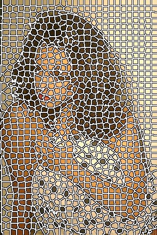
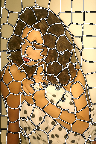
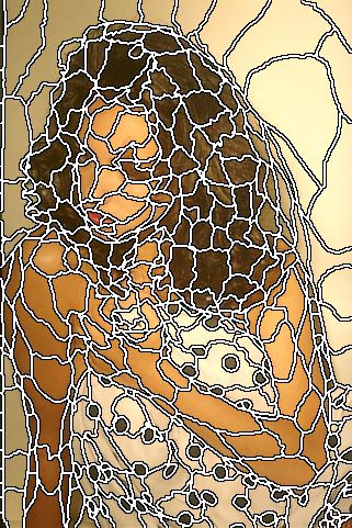
(a) Too many superpixels	(b) Loss of detail	(c) Just right

Figure 1: The dilemma of choosing the right superpixel size - (a) retain detail and obtain too many superpixels, or (b) lose structures smaller than the superpixel size? Usually, several sizes are tried before choosing one that suits the need. (c) With adaptels, the choice of size is automatic, the number of superpixels is kept small, and all the advantages of a superpixel-based over-segmentation are retained. The number of segments in (c) is less than 50% of those in (a).

Compared to the state-of-the-art, our method offers several advantages. There is no need to choose the size of the segments - their size is generated automatically. Similarly, the location and number of segments are automatically chosen to conform to the image content. Our algorithm minimizes the number of image segments while upper-bounding the information contained in them. This upper bound is the only parameter we need to set. Additionally, our algorithm grows segments ensuring connectivity. The resulting segments, adaptels, are compact, with a limited degree of adjacency. Finally, the algorithm complexity is linear in the number of pixels and runs in real-time without using any specialized hardware or optimization.

The rest of the paper is as follows. Section 2 surveys the related background work. We present a formal explanation of adaptels and the corresponding algorithm in Section 3. In Section 4 we compare adaptels to other methods. We show that our method performs better than others on standard metrics. Section 6 concludes the paper.

2 Related work

Superpixel segmentation is an active research topic with large number of proposed methods. This review is not exhaustive but an attempt is being made to cover prominent algorithms that encompass a wide range of approaches for creating superpixels. We also include traditional segmentation algorithms that do not aim to create uniformly sized segments.

One of the earliest graph-based approaches, the Normalized cuts algorithm [25], creates NCUTS superpixels by recursively computing normalized cuts for the pixel graph. Felzenszwalb and Huttenlocher [11] propose a minimum spanning tree based EGB segmentation approach, which is computationally much simpler. To create segments, which are essentially sub-trees, a stopping criterion is used to prevent the tree-growing from spanning the entire image with a single tree. Unlike NCUTS, EGB does not create uniformly-sized superpixels. Moore et al. [21] generate SLAT superpixels by finding the shortest paths that split the image into vertical and horizontal strips. Similarly, Zhang et al. [32] create SPBO superpixels by applying horizontal and vertical graph-cuts to overlapping strips of an image. Instead of finding cuts on an image, Veskler et al. [28], generate GCUT superpixels by stitching together overlapping image patches using graph cuts optimization. More recently, Liu et al. [16] present another graph-based approach to create ERS superpixels that connects subgraphs by maximising the entropy rate of a random walk.

There are several other algorithms that are not graph-based. The watershed algorithm [29] accumulates similar pixels starting from local minima to find WSHED segments. The mean shift algorithm [10] iteratively locates local maxima of a density function in color and image plane space. Pixels that lead to the same local maximum belong to the same MSHIFT segment. Quick-shift [27] creates QSHIFT superpixels by seeking local maxima like MSHIFT but is more efficient in terms of computation. The Turbopixels algorithm [14] generates TPIX superpixels by progressively dilating pixel seeds located at regular grid centers using a level-set approach. Like TPIX, the Simple Linear Iterative Clustering (SLIC) algorithm [8] also relies on starting seed pixels chosen at regular grid intervals. It performs a localized k-means optimization in the five-dimensional CIELAB color and image space to cluster pixels into SLIC superpixels. Two recent variants of SLIC are presented by Li and Chen [15], and by Liu et al. [17]. The former projects the five-dimensional space of spatial coordinates and color on a ten-dimensional space and the latter projects it to a two-dimensional space before performing $k$-means clustering. Both the works show improvement in segmentation quality.

Method	EGB	MSHIFT	WSHED	QSHIFT	GEOD	NCUTS	SLAT	SPBO	GCUT	TPIX	SLIC	SEEDS	ERS	LSC	MSLIC	Adaptels
Reference	[11]	[10]	[29]	[27]	[30]	[25]	[21]	[32]	[28]	[14]	[8]	[26]	[16]	[15]	[17]	$-$
Agglomerative	$\bullet$	$\bullet$	$\bullet$	$\bullet$	$\bullet$	$\cdot$	$\cdot$	$\cdot$	$\cdot$	$\bullet$	$\cdot$	$\cdot$	$\cdot$	$\cdot$	$\cdot$	$\bullet$
Divisive	$\cdot$	$\cdot$	$\cdot$	$\cdot$	$\bullet$	$\bullet$	$\bullet$	$\bullet$	$\cdot$	$\cdot$	$\cdot$	$\bullet$	$\cdot$	$\cdot$	$\cdot$	$\cdot$
Graph-based	$\bullet$	$\cdot$	$\cdot$	$\cdot$	$\cdot$	$\bullet$	$\cdot$	$\bullet$	$\bullet$	$\cdot$	$\cdot$	$\cdot$	$\bullet$	$\cdot$	$\cdot$	$\cdot$
Patch-based	$\cdot$	$\cdot$	$\cdot$	$\cdot$	$\cdot$	$\cdot$	$\cdot$	$\cdot$	$\bullet$	$\cdot$	$\cdot$	$\cdot$	$\cdot$	$\cdot$	$\cdot$	$\cdot$
Center-seeking	$\cdot$	$\bullet$	$\cdot$	$\bullet$	$\bullet$	$\cdot$	$\cdot$	$\cdot$	$\cdot$	$\cdot$	$\bullet$	$\cdot$	$\cdot$	$\bullet$	$\bullet$	$\cdot$
Border seeking	$\cdot$	$\cdot$	$\bullet$	$\cdot$	$\cdot$	$\cdot$	$\cdot$	$\cdot$	$\cdot$	$\bullet$	$\cdot$	$\cdot$	$\cdot$	$\cdot$	$\cdot$	$\bullet$
Iterative	$\cdot$	$\cdot$	$\cdot$	$\cdot$	$\bullet$	$\cdot$	$\cdot$	$\cdot$	$\cdot$	$\cdot$	$\bullet$	$\bullet$	$\cdot$	$\bullet$	$\bullet$	$\cdot$
Grid seeding	$\cdot$	$\cdot$	$\cdot$	$\cdot$	$\bullet$	$\cdot$	$\bullet$	$\bullet$	$\bullet$	$\bullet$	$\bullet$	$\bullet$	$\cdot$	$\bullet$	$\bullet$	$\cdot$
Uniform size	$\cdot$	$\cdot$	$\cdot$	$\cdot$	$\cdot$	$\bullet$	$\bullet$	$\bullet$	$\bullet$	$\bullet$	$\bullet$	$\bullet$	$\cdot$	$\bullet$	$\bullet$	$\cdot$
Real-time	$\bullet$	$\cdot$	$\bullet$	$\cdot$	$\cdot$	$\cdot$	$\cdot$	$\cdot$	$\cdot$	$\cdot$	$\bullet$	$\bullet$	$\cdot$	$\cdot$	$\bullet$	$\bullet$

Table 1: A comparison by algorithmic properties of the different superpixel methods considered in this review. A large dot indicates the presence of the corresponding characteristic.

Wang et al. [30] present a geodesic distance based algorithm that generates GEOD superpixels of varying size based on image content but is slow in practice. A more recent non-graph algorithm [26] generates SEEDS superpixels by iteratively improving an initial rectangular approximation of superpixels using coarse to fine pixel exchanges with neighboring superpixels.

A comparative summary of the state-of-the-art is presented in Table 1. EGB, MSHIFT, and WSHED are traditional segmentation algorithms that do not aim for uniformly-sized, compact segments. Of the others, NCUTS, SLAT, TPIX, SLIC, and SPBO are more compact. SLIC, ERS, and SEEDS perform well on benchmark comparisons. EGB, SLIC, and SEEDS are the fastest in computation. TPIX, SLIC, ERS, and SEEDS allow the user control over the number of output segments. This last property of superpixels is important because it lets the user choose the size of the superpixels based on needs of the application. By doing so, the user accepts to lose structural information finer than the superpixel size. The Adaptel algorithm is the only one we are aware of that frees the user from making this choice, and yet offers compactness, high precision, and computational efficiency.

3 The proposed method

Image segmentation is the procedure of grouping the pixels $\mathcal{P}$ of an image into a number of connected components $\{\mathcal{A}_{k}\}_{k=1}^{K}$ that form a partition. Our goal is to minimize the number of segments $K$ while bounding the amount of information each one contains. We therefore want to find

$$\min_{\{\mathcal{A}_{k}\}_{k=1}^{K}}\!\!\!K\!\!\!\!\!\!\!\!\!\qquad\operatorname{s.t.} \bigcup_{k}\mathcal{A}_{k}\!\!=\!\!\mathcal{P},\!\!\!\!\!\quad\mathcal{A}_{j}\!\cap\!A_{k}\!\!=\!\!\emptyset\quad\!\!\forall j\!\!\neq\!\!k,$$ (1a)

$$\min_{\{\mathcal{A}_{k}\}_{k=1}^{K}}\!\!\!K\!\!\!\!\!\!\!\!\!\qquad\operatorname{s.t.} \mathrm{Connected}(\mathcal{A}_{k})=1\ \forall k,$$ (1b)

$$\min_{\{\mathcal{A}_{k}\}_{k=1}^{K}}\!\!\!K\!\!\!\!\!\!\!\!\!\qquad\operatorname{s.t.} I(\mathcal{A}_{k})\leq T\ \forall k.$$ (1c)

The resulting $\mathcal{A}_{k}$ are the adaptels. Line (1a) ensures that they form an image-partition. Line (1b) enforces connectivity of every adaptel. Line (1c) constraints the amount of information contained in every adaptel to be less than a threshold $T$, given in bits. The value of $T$ is the only hyperparameter of our method. It controls the number of adaptels in the resulting segmentations.

We define the information contained in an adaptel to be the Shannon self-information

$$I(\mathcal{A}_{k})=\min_{\theta}-\log P(\mathcal{A}_{k};\theta),$$ (2)

for a given family of probability distributions $P$ parameterized by a vector $\theta$. $I(\mathcal{A}_{k})$ measures the complexity of an adaptel $\mathcal{A}_{k}$ by finding the distribution $P(\cdot;\theta)$ from the family $P$ that best fits its content and then computing the number of bits required to encode $\mathcal{A}_{k}$ under that distribution. Instead of imposing a fixed criterion on complexity, our method is flexible enough to allow the user to define what complexity means by choosing the proper family of distributions $P$: simple regions are those that are likely to happen under $P$, while complex regions are those with low probability. To illustrate, a Gaussian distribution over the color space will consider homogeneous-looking regions to be simple, while for a bimodal distribution simple means regions made up of two colors. By thresholding the information content, we make adaptels small in areas of large complexity and vice versa.

The joint probability $P(\mathcal{A}_{k};\theta)$ depends on tens or hundreds of variables, which makes its exact representation and computation intractable. We will thus make the usual i.i.d. assumption over pixels inside each adaptel and factorize the joint probability as

$$I(\mathcal{A}_{k})=\min_{\theta}-\sum_{i\in\mathcal{A}_{k}}\log P(\mathbf{x}_{i};\theta),$$ (3)

where the feature vector $\mathbf{x}_{i}$ for pixel $i$ contains a description of its visual appearance and position.

3.1 Adaptel Algorithm

The minimization problem of Eq. (1c) is NP-hard and intractable even for small images. We approach the problem in an approximate manner and grow the adaptels as shown in Algorithm 1.

Every adaptel $\mathcal{A}_{k}$ starts growing from a single pixel called its seed, which is used to initialize a candidate map $C$. At every iteration we take the pixel $c$ from the candidate map $C$ that contributes the least information to the adaptel. We add $c$ to the adaptel and update the map $C$ with the neighbor pixels of $c$ as possible candidates. The adaptel stops growing when the information threshold $T$ is reached. This growing procedure ensures the conditions of connectivity (1b) and bounded information (1c).

To mitigate the greediness of our algorithm, we allow neighboring adaptels to compete with each other for pixel ownership. This helps ensure that pixels are assigned to the most appropriate adaptel and not to the one that reaches them first. To this end, we keep a map  $D$ that stores the accumulated information contribution of each pixel when it joins an adaptel (line 6 in Algo. 1). Candidate pixels are reassigned to the current adaptel if their new information contribution is lower than the one stored in the map $D$ (line 9 in Algo. 1). As an additional consequence, the information map $D$ also encourages the compactness of the adaptels.

Algorithm 1 GrowAdaptel: Growing an adaptel $\mathcal{A}_{k}$.

0:  The upper bound $T$, the adaptel seed pixel $s$, the information map $D$, connected neighbors $\mathcal{N}$ for each pixel

0:  The adaptel $\mathcal{A}_{k}$, updated information map $D$

1:  Initialize adaptel $\mathcal{A}_{k}\leftarrow\emptyset$

2:  Initialize candidate map $C[s]=I\left(\{s\}\right)$

3:  while $C$ is not empty do

4:     Get best candidate $c\leftarrow\operatorname*{arg\,min}_{c}C[c]$

5:     Put candidate in adaptel $\mathcal{A}_{k}\leftarrow\mathcal{A}_{k}\cup\{c\}$

6:     Update information map $D[c]\leftarrow C[c]$

7:     for $c^{\prime}\in\mathcal{N}(c)$ do

8:        Compute information of the adaptel with the new candidate $e\leftarrow I\left(\mathcal{A}_{k}\cup\{c^{\prime}\}\right)$

9:        Update candidate map $C[c^{\prime}]\leftarrow e$ if $e<T$ and $e<D[c^{\prime}]$

10:     end for

11:     Remove $c$ from $C$

12:  end while

13:  return  $\mathcal{A}_{k},D$

Algorithm 2 repeats this procedure as many times as necessary until the whole image is partitioned, thus meeting the constraint of Eq. (1a). The seed of every adaptel is chosen among the border pixels of the previous ones, stored in the list $\mathcal{S}$. We set the seed of the first adaptel to be the central pixel of the image. Fig. 2 illustrates the complete procedure.

Algorithm 2 The Adaptel algorithm.

0:  Information upper bound $T$, seed pixel $s$

0:  Set of adaptels $\aleph$

1:  $\aleph\leftarrow\emptyset$

2:  Set of seeds $\mathcal{S}\leftarrow\{s\}$

3:  Initialize information map $D[:]\leftarrow\infty$

4:  while $\mathcal{S}$ is not empty do

5:     Get seed $s\in\mathcal{S}$

6:     $\mathcal{A}_{k},D\leftarrow\textsc{GrowAdaptel}(T,s,D)$

7:     $\aleph\leftarrow\aleph\cup\{\mathcal{A}_{k}\}$

8:     $\mathcal{S}\leftarrow\mathcal{S}\cup\left\{\textrm{Pixels bordering }\mathcal{A}_{k}\right\}$

9:     Remove seeds from $\mathcal{S}$ that are assigned to an adaptel $\mathcal{S}\leftarrow\mathcal{S}-\bigcup_{\mathcal{A}_{k}\in\aleph}\mathcal{A}_{k}$

10:  end while

11:  return  $\aleph$

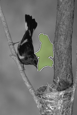
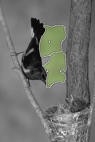
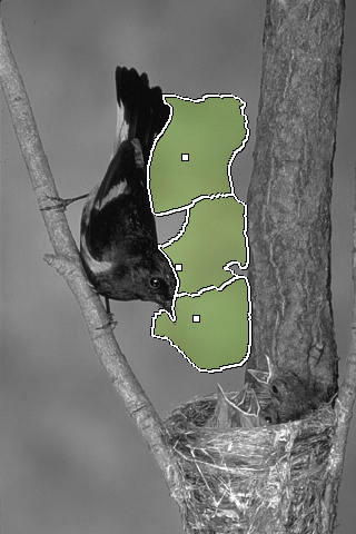
(a)	(b)	(c)	(d)

Figure 2: The process of segmenting an image. (a) The first adaptel is grown from the center seed (white square) outwards by gathering neighboring pixels in order of increasing information until the information upper-bound $T$ is reached. (b and c) Subsequent adaptels are grown using pixels at the borders of the previous adaptels as seeds (white squares). As seen, the new adaptels capture pixels from the previous ones, resulting in constantly evolving segment boundaries. This mitigates the greediness of the algorithm and encourages boundary adherence. (d) Final segmented image.

By growing the adaptels using the least informative candidate until they reach the information threshold, we are maximizing their sizes. In turn, this minimizes the number of adaptels, as expressed in the initial formulation of our problem (Eq. (1c)).

Computing the information in lines 2 and 8 of Algorithm 1 depends on the specific family of probability distributions chosen. In the next section we introduce the family of probability distributions we use in our experiments, and describe how to compute the information of growing adaptels with it.

3.2 Accommodating the visual complexity of natural images

The Adaptel algorithm is agnostic to the family of probability distributions $P$ used to describe complexity. Different families lead to different styles of superpixels. However, looking for the suitable distribution for every particular case is hard. In this section we introduce a family of probability distributions that are suitable for a wide range of applications.

In most real-world cases, complexity is perceived as visual variability. Homogeneous, constant-color regions are perceived as simple, while textured regions are complex. Based on this idea, we look for a unimodal family of distributions in the space of visual features.

The most straightforward family of distributions in this category are the multivariate normal distributions. However, the normal distribution over-penalizes pixels that are visually far from the mean, while it under-penalizes pixels close to the mean. This leads to extreme segmentations with very large adaptels in homogeneous areas and very small ones in textured areas.

A unimodal family with smoother behavior is the multivariate double exponential distribution

$$P_{mde}(\mathbf{x};\bm{\mu},\sigma)=\frac{1}{Z}\exp\left(-{\sqrt{\dfrac{(\mathbf{x}-\bm{\mu})^{T}(\mathbf{x}-\bm{\mu)}}{\sigma^{2}}}}\right),$$ (4)

where $Z$ is the normalization factor and $\mathbf{x}$ is the vector of visual features. Unlike the normal, the double exponential has a softer decay when moving away from the mean, and it does not penalize variability as much. Using it yields better-behaved segmentations, with more regularity on the sizes of the adaptels. This will be our distribution of choice for the remainder of this paper.

The double exponential distribution is parameterized by the mean vector $\bm{\mu}$ and the scalar variance $\sigma^{2}$. We fix the variance $\sigma^{2}$ so that $P_{mde}(\bm{\mu};\bm{\mu},\sigma)=1$, leaving remaining vector $\bm{\mu}$ as the only parameter $\theta$ of our family. Computing the information of an adaptel with Eq. (3) requires finding the parameter $\theta$ that best fits the content of the adaptel. With the multivariate double exponential, the best fit is given by the mean of the observations inside the adaptel,

$$\theta^{*}(\mathcal{A}_{k})=\dfrac{1}{|\mathcal{A}_{k}|}\sum_{i\in\mathcal{A}_{k}}\mathbf{x}_{i},$$ (5)

and the information is

$$I(\mathcal{A}_{k})=-\log\sum_{i\in\mathcal{A}_{k}}P_{mde}(\mathbf{x}_{k};\theta^{*}(\mathcal{A}_{k})).$$ (6)

These two equations give the implementation of lines 2 and 8 of Algorithm 1. For efficiency, we do not compute the information from scratch at every iteration in line 8, but perform online updates starting from previous estimations of the mean and the information.

All the results shown in this paper are obtained with this family of double exponential distributions with fixed $\sigma$. Reasonable values of the upper-bound $T$ for natural images with this family are in range $(50,150)$ bits. Source code will be made available upon publication of the paper.

NCUTS [25]	EGB [11]	TPIX [14]	GCUT [28]	SLIC [8]	SEEDS [26]	ERS [16]	LSC [15]	Adaptels

Figure 3: Visual comparison of different segmentation algorithms. In the zoomed-in regions notice how well adaptels adhere to each region of the image according to its local structure. Results for adaptels use a threshold $T=90\,\textrm{bits}$ and the initial seed is the central pixel of each image.

4 Comparison

We assess the power of the information uniformity assumption against the standard size uniformity assumption. We compare adaptels to several state-of-the-art superpixel methods: EGB [11], TPIX [14], GCUT [28] SLIC [8], SEEDS [26], ERS [16] and LSC [15]. We used implementations available online for all methods [1, 2, 3, 4, 5, 6, 7].

We use the Berkeley 300 dataset [19] with its color and gray scale groundtruth images (3269 in total). Fig. 4 depicts results for the entire range of 50 to 2000 superpixels, corresponding to an image simplification ranging from four to two orders of magnitude.

4.1 Under-segmentation error

Under-segmentation error measures the overlap error, also termed “leak” or “bleeding” between groundtruth and superpixel segments. The computation of under-segmentation error as presented in TPIX and later in SLIC penalizes every overlapping error twice, on either side of the erring superpixel as pointed out by Neubert and Protzel [23]. We compute the Corrected Under-Segmentation Error (CUSE) [23]. CUSE for each image is computed as the sum of overlap error for each superpixel segment $S_{k}$:

$${CUSE}=\frac{1}{N}\sum^{K}_{k=1}|G^{\ast}(S_{k})\cup S_{k}-G^{\ast}(S_{k})|$$ (7)

where $G^{\ast}(S_{k})=\operatorname*{arg\,max}_{j}{(G_{j}\cap S_{k})}$ is the ground truth segment with which segment $S_{k}$ has the maximum overlap.

A related comparison measure introduced by ERS [16], and also computed by SEEDS [26], is Achievable Segmentation Accuracy (ASA), expressed as: ${ASA}=\frac{1}{N}\sum^{K}_{k=1}G^{\ast}(S_{k})$. We see that ASA is simply the complement of CUSE - for any given pair of superpixel and ground truth labels, the two values add up to $1$. We therefore only show the plot for CUSE in Fig. 4. Adaptels show the least error of all for most superpixel sizes.

4.2 Boundary recall

Recall is the ratio of the true positives ($TP$) to the sum of true positives and false negatives ($FN$). We represent boundary maps, which have the same size and dimensions as the corresponding image, for superpixel segmentation as $b^{S}_{i}$, and for ground truth as $b^{G}_{i}$, such that the value at pixel position $i$ is $1$ in the presence of a boundary and $0$ otherwise. Boundary recall is computed for each pair of input image and groundtruth in the same way as done by TPIX [14], SLIC [8], SEEDS [26], and ERS [16]:

$${Recall}=\frac{TP}{TP+FN}=\frac{\sum^{N}_{i=1}{\mathds{I}_{j\in\mathcal{N}(i,\epsilon)}(b^{G}_{i}\land b^{S}_{j})}}{\sum^{N}_{i=1}{\mathds{I}(b^{G}_{i})}}$$ (8)

where $\land$ represents a logical and operation, $\mathds{I}$ represents a function that returns $1$ if the entity passed to the function is greater than $0$, and $\mathcal{N}(i,\epsilon)$ is the neighborhood of $i$ at range $\epsilon$. The denominator term $TP+FN$ is then simply the number of all boundary pixels. We use $\epsilon=2$ as done in the past [8, 16, 26, 23].

4.3 Boundary precision

By treating a segmentation algorithm as a boundary detection algorithm, superpixel algorithms compute boundary recall for comparison. But recall alone can be misleading since it is possible to have a very high recall with extremely poor precision. For the task of segmentation, it is well established in literature [18, 9] that recall has to be regarded in conjunction with precision.

In this paper, we compute precision, which is often missing in previous works (TP [14], SLIC [8], SEEDS [26], ERS [16]). To compute precision, we need to know the number of false positives $FP$, which is the number of superpixel boundary pixels in the $\epsilon$ neighbourhood that are not true positives:

$$FP=\sum^{N}_{i=1}{\left[1-\mathds{I}_{j\in\mathcal{N}(i,\epsilon)}(b^{G}_{i}\land b^{S}_{j})\right]}$$ (9)

Knowing $FN$ allows us to compute precision as ${Precision}=TP/(TP+FP)$ where $TP$ is the same as the numerator term of Eq. 8.

4.4 Precision-recall and F-measure

Using the boundary recall and precision values, we are able to plot the more conclusive curves of Precision vs. Recall and F-measure versus number of superpixels, shown in Fig. 4. These plots prove the superiority of adaptels over other methods.

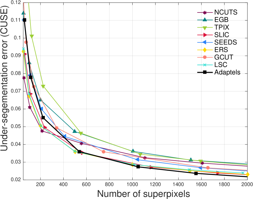
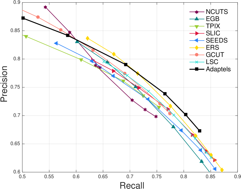
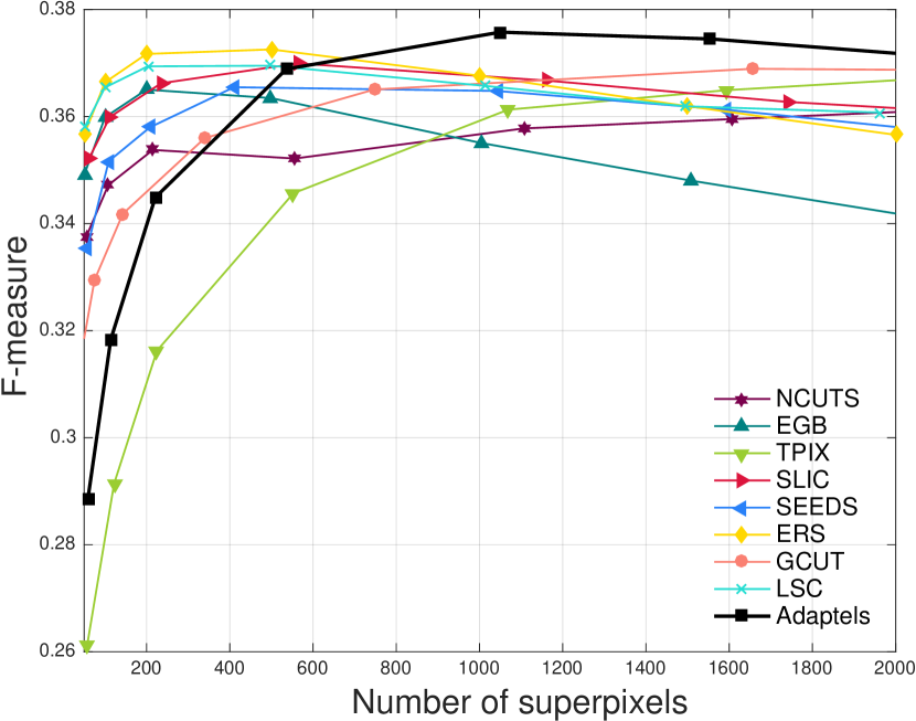
Figure 4: (Top) The under-segmentation error (CUSE) of adaptels is the lowest. (Middle) Adaptels have a better precision-versus recall performance, and (Bottom) a better F-measure than the state-of-the-art. The values at 1000 superpixels are compared in Table 2.

	CUSE	F-measure	Speed (fps)
NCUTS	0.0325	0.3578	-
EGB	0.0361	0.3551	12.5
TPIX	0.0345	0.3613	0.2
GCUTS	0.0358	0.3651	0.5
SLIC	0.0274	0.3667	13.9
SEEDS	0.0313	0.3648	18.1
ERS	0.0286	0.3676	1.2
LSC	0.0286	0.3657	3.2
Adaptels	0.0273	0.3758	14.7

Table 2: Every row shows the values computed for a given algorithm for the corresponding metric from Fig. 4 for 1000 superpixels on images of size $321\times 481$ pixels. The best values are highlighted in bold. Adaptels outperform the other methods on these metrics. NCUTS is far slower than other methods, taking over a hundred seconds for a single image. Apart from SEEDS, whose timing varies from 12 to 24 fps depending on the number of superpixels, the Adaptel algorithm is the fastest method, capable of processing nearly 15 fps on a regular laptop.

4.5 Computational efficiency

We measured the speed of every method for images of size $481\times 321$. We present the average number of frames-per-second (fps) in Table 2. All of the algorithms run on the same hardware (2.6 GHz Intel Core i7 processor, with 16 GB of RAM, running OSX). We do not use any parallelization, GPU processing, or dedicated hardware for any of the algorithms. The speed of SEEDS varies from 12 to 24 fps for different number of superpixels. The speed of other algorithms, including Adaptels, is independent of the number of superpixels. Barring SEEDS, the Adaptel is the fastest segmentation algorithm.

4.6 Discussion of results

Adaptels exhibit the lowest under-segmentation error of all methods compared with (Fig. 4). As is customary for any detection problem, we compute boundary precision along with boundary recall. The two measures independently are insufficient to convey the quality of a segmentation algorithm. For instance, it is possible to have a very high recall if all superpixels are of size $1$. Similarly, it is possible to have high precision even if a single boundary pixel is correctly detected and there are no false positives. Considering the two values together avoids biasing the evaluations towards methods that generate noisy or jagged segment boundaries, e.g. EGB, SLIC, ERS, and LSC.

With the help of these two measures we plot the precision-recall curve and F-measure curve shown in Fig. 4. These curves offer a fair and conclusive comparison of the segmentation methods. In both these plots we notice that adaptels outperform the state-of-the-art. Additionally, the numbers provided in Table 2 show that adaptels not only outperform the state-of-the-art in terms of segmentation quality but also in terms of computational efficiency.

5 Video adaptels

It is trivial to extend the Adaptel algorithm to higher dimensional data like image stacks and video volumes. Adaptel segmentation starts at the center of the volume. Instead of looking in the 2D neighborhood for growing an Adaptel, connected pixels are obtained from a 3D neighborhood. So, apart from this change to $\mathcal{N}$ and the necessary changes to the maps $C$ and $D$, the other steps remain the same in algorithms 1 and 2 for 3D segmentation. Fig. 5 shows an example of a segmented video volume with the cross-sections along the time axis. Fig. 6 shows a few individual frames from the same video volume. Just as in 2D, the object boundaries are also well-adhered to in the 3D case. The computational complexity remains linear in the number of voxels in the volume.

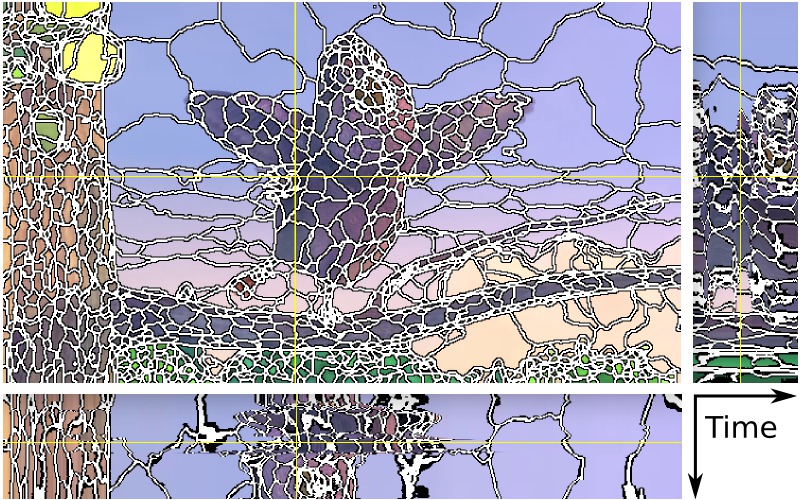
Figure 5: Adaptel segmention in 3D. This image shows a cross-hairs based 3D section of the segmented video volume of 100 frames seen from the right (Y-Time plane) and bottom (X-Time plane). The segmented video is provided in the supplementary material.

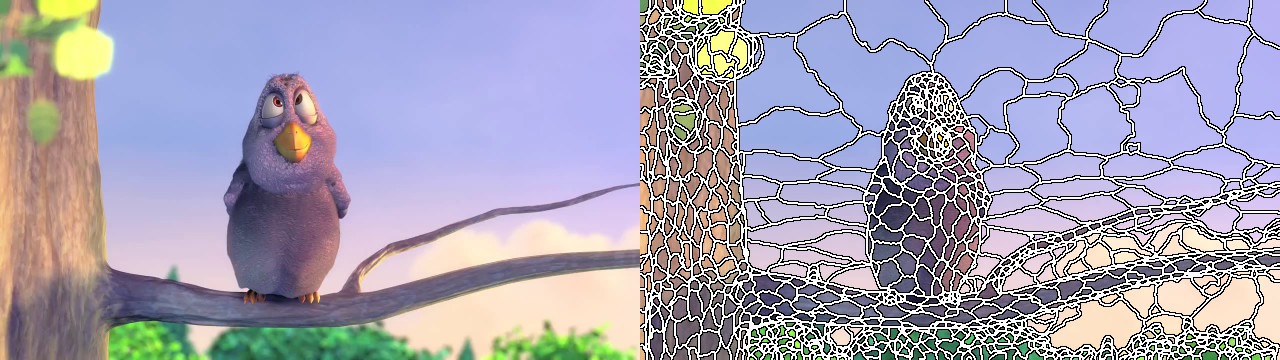
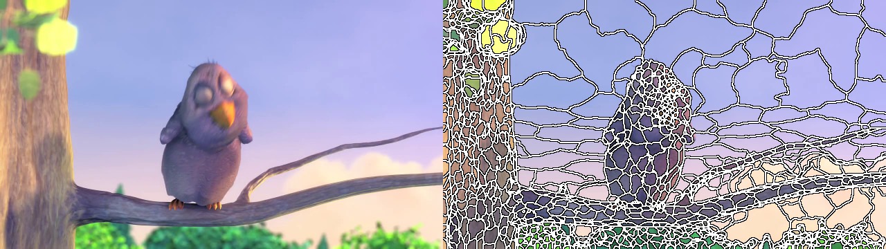
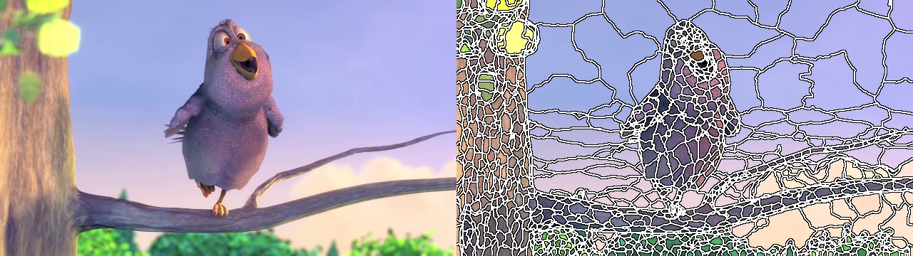
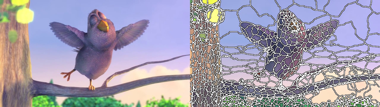
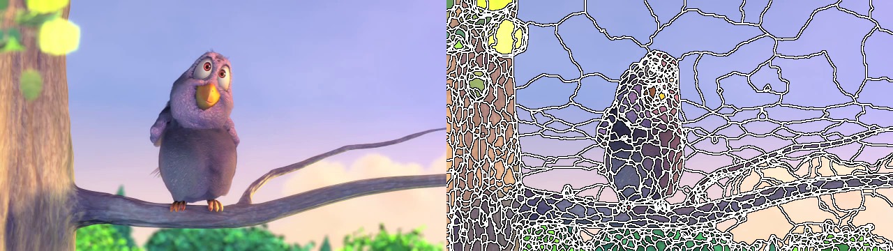
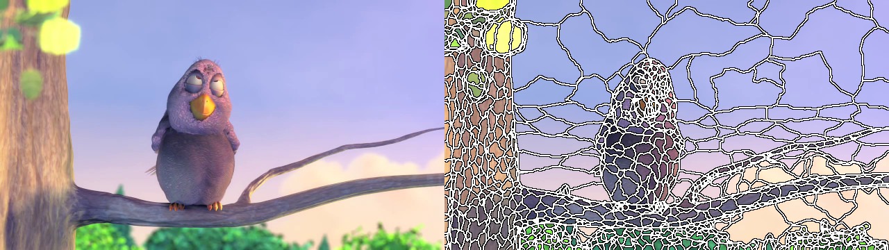
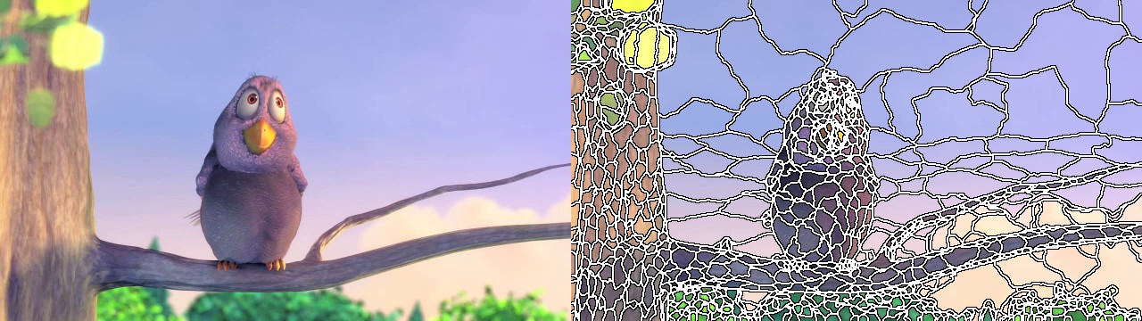
Figure 6: Supervoxel segmentation. The images here show a few frames of the video volume of Fig. 5 that has been segmented using the 3D extension of the Adaptel algorithm.

6 Conclusion

We introduced an information-theoretic approach for creating image segments which we call Adaptels. Instead of assuming uniformity in size or shape, we assume information uniformity. This leads to segments that change their size according to the local image complexity as defined by a family of probability distributions. We have used the double exponential distribution to encode complexity in natural images. For other types of images, our approach offers the possibility of using application-specific distributions.

The experimental comparison proves the superiority of adaptels. Our algorithm has the lowest under-segmentation error, is the best in both precision versus recall performance, as well as in terms of F-measure. The algorithm is linear in the number of pixels, and is among the fastest methods considered. It is simple to use, requiring only one parameter: the upper-bound of the information contained in every segment. There is no need to set the superpixel size or choose seeds a priori, since both of these are achieved automatically by the algorithm. Finally, the algorithm is easily extended to higher dimensional data.

References

- [1] http://cs.brown.edu/ pff/segment/.
- [2] http://ivrl.epfl.ch/research/superpixels.
- [3] http://jschenthu.weebly.com/projects.html.
- [4] https://github.com/akanazawa/collective-classification/tree/master/segmentation.
- [5] http://www.csd.uwo.ca/faculty/olga/.
- [6] http://www.cs.toronto.edu/ babalex/research.html.
- [7] http://www.mvdblive.org/seeds/.
- [8] R. Achanta, A. Shaji, K. Smith, A. Lucchi, P. Fua, and S. Süsstrunk. SLIC superpixels compared to state-of-the-art superpixel methods. IEEE Transactions on Pattern Analysis and Machine Intelligence, 34(11):2274—2282, 2012.
- [9] P. Arbelaez, M. Maire, C. Fowlkes, and J. Malik. Contour detection and hierarchical image segmentation. IEEE Transactions on Pattern Analysis and Machine Intelligence (PAMI), 33(5):898–916, May 2011.
- [10] D. Comaniciu and P. Meer. Mean shift: a robust approach toward feature space analysis. IEEE Transactions on Pattern Analysis and Machine Intelligence, 24(5):603–619, May 2002.
- [11] P. Felzenszwalb and D. Huttenlocher. Efficient graph-based image segmentation. International Journal of Computer Vision (IJCV), 59(2):167–181, September 2004.
- [12] B. Fulkerson, A. Vedaldi, and S. Soatto. Class segmentation and object localization with superpixel neighborhoods. In International Conference on Computer Vision (ICCV), 2009.
- [13] S. Gould, J. Rodgers, D. Cohen, G. Elidan, and D. Koller. Multi-class segmentation with relative location prior. International Journal of Computer Vision (IJCV), 80(3):300–316, 2008.
- [14] A. Levinshtein, A. Stere, K. Kutulakos, D. Fleet, S. Dickinson, and K. Siddiqi. Turbopixels: Fast superpixels using geometric flows. IEEE Transactions on Pattern Analysis and Machine Intelligence (PAMI), 2009.
- [15] Z. Li and J. Chen. Superpixel segmentation using linear spectral clustering. In 2015 IEEE Conference on Computer Vision and Pattern Recognition (CVPR), pages 1356–1363, June 2015.
- [16] M.-Y. Liu, O. Tuzel, S. Ramalingam, and R. Chellappa. Entropy rate superpixel segmentation. In IEEE Conference on Computer Vision and Pattern Recognition (CVPR), 2011.
- [17] Y.-J. Liu, C.-C. Yu, M.-J. Yu, and Y. He. Manifold slic: A fast method to compute content-sensitive superpixels. In The IEEE Conference on Computer Vision and Pattern Recognition (CVPR), June 2016.
- [18] D. Martin, C. Fowlkes, and J. Malik. Learning to detect natural image boundaries using local brightness, color, and texture cues. IEEE Transactions on Pattern Analysis Machine Intelligence (PAMI), 26(5):530–549, 2004.
- [19] D. Martin, C. Fowlkes, D. Tal, and J. Malik. A database of human segmented natural images and its application to evaluating segmentation algorithms and measuring ecological statistics. In IEEE International Conference on Computer Vision (ICCV), July 2001.
- [20] M. Menze and A. Geiger. Object scene flow for autonomous vehicles. In Conference on Computer Vision and Pattern Recognition (CVPR), 2015.
- [21] A. Moore, S. Prince, J. Warrell, U. Mohammed, and G. Jones. Superpixel Lattices. In IEEE Computer Vision and Pattern Recognition (CVPR), 2008.
- [22] G. Mori. Guiding model search using segmentation. In IEEE International Conference on Computer Vision (ICCV), 2005.
- [23] P. Neubert and P. Protzel. Superpixel benchmark and comparison. In Proc. of Forum Bildverarbeitun, Regensburg, Germany, 2012.
- [24] X. Ren and J. Malik. Learning a classification model for segmentation. In IEEE Conference on Computer Vision (CVPR), 2003.
- [25] J. Shi and J. Malik. Normalized cuts and image segmentation. IEEE Transactions on Pattern Analysis and Machine Intelligence (PAMI), 22(8):888–905, Aug 2000.
- [26] M. Van den Bergh, X. Boix, G. Roig, and L. Van Gool. SEEDS: Superpixels extracted via energy-driven sampling. International Journal of Computer Vision, 111(3):298–314, 2015.
- [27] A. Vedaldi and S. Soatto. Quick shift and kernel methods for mode seeking. In European Conference on Computer Vision (ECCV), 2008.
- [28] O. Veksler, Y. Boykov, and P. Mehrani. Superpixels and supervoxels in an energy optimization framework. In European Conference on Computer Vision (ECCV), 2010.
- [29] L. Vincent and P. Soille. Watersheds in digital spaces: An efficient algorithm based on immersion simulations. IEEE Transactions on Pattern Analalysis and Machine Intelligence, 13(6):583–598, 1991.
- [30] P. Wang, G. Zeng, R. Gan, J. Wang, and H. Zha. Structure-sensitive superpixels via geodesic distance. International Journal of Computer Vision, 103(1):1–21, 2013.
- [31] S. Wang, H. Lu, F. Yang, and M.-H. Yang. Superpixel tracking. In IEEE International Conference on Computer Vision (ICCV), Nov 2011.
- [32] Y. Zhang, R. Hartley, J. Mashford, and S. Burn. Superpixels via pseudo-boolean optimization. In IEEE International Conference on Computer Vision (ICCV), Nov 2011.
- [33] C. L. Zitnick and S. B. Kang. Stereo for image-based rendering using image over-segmentation. International Journal of Computer Vision (IJCV), 75:49–65, October 2007.