Positive Quantum Magnetoresistance in Tilted Magnetic Field.

Abstract

Transport properties of highly mobile 2D electrons are studied in symmetric GaAs quantum wells placed in titled magnetic fields. Quantum positive magnetoresistance (QPMR) is observed in magnetic fields perpendicular to the 2D layer. Application of in-plane magnetic field produces a dramatic decrease of the QPMR. This decrease correlates strongly with the reduction of the amplitude of Shubnikov de Haas resistance oscillations due to modification of the electron spectrum via enhanced Zeeman splitting. Surprisingly no quantization of the spectrum is detected when the Zeeman energy exceeds the half of the cyclotron energy suggesting an abrupt transformation of the electron dynamics. Observed angular evolution of QPMR implies $\displaystyle strong$ mixing between spin subbands. Theoretical estimations indicate that in the presence of spin-orbital interaction the elastic impurity scattering provides significant contribution to the spin mixing in GaAs quantum wells at high filling factors.

I Introduction

The orbital quantization of electron motion in magnetic fields generates a great variety of fascinating transport phenomena observed in condensed materials. Shubnikov-de Haas (SdH) resistance oscillations¹ and Quantum Hall Effect (QHE)² are famous examples. Spin degrees of freedom enrich the electron response.^{3; 4} In two dimensional (2D) electron systems the orbital quantization is due to the component of the magnetic field, $\displaystyle B_{\perp}$, which is perpendicular to 2D layer⁵ whereas the spin degrees of freedom are affected mostly by the total magnetic field, $\displaystyle B$.⁶ An increase of the in-plane magnetic field produces, thus, an enhancement of the spin splitting (Zeeman effect), $\displaystyle\Delta_{Z}=\mu gB$, with respect to the cyclotron energy, $\displaystyle\Delta_{C}=\hbar\omega_{c}$. Here $\displaystyle\mu$ is Bohr magneton, $\displaystyle g$ is $\displaystyle g$-factor, $\displaystyle\omega_{c}=eB_{\perp}/m=eBcos(\alpha)/m$ is cyclotron frequency, $\displaystyle m$ is electron effective mass and $\displaystyle\alpha$ is the angle between magnetic field $\displaystyle\vec{B}$ and the normal $\displaystyle\vec{n}$ to 2D layer. At a critical angle $\displaystyle\alpha_{c}$ corresponding to the condition:

$$\displaystyle\Delta_{Z}=\frac{\Delta_{C}}{2}\Leftrightarrow cos(\alpha_{c})=\frac{gm}{m_{0}},$$ (1)

where parameter $\displaystyle m_{0}$ is mass of free electron, quantum levels are equally separated by $\displaystyle\hbar\omega_{c}/2$ and the amplitude of the fundamental harmonic of SdH oscillations, $\displaystyle A_{SdH}$, is zero. This property is the basis of a powerful transport method (coincidence method) for the study of the spin degrees of freedom of 2D electrons.^{3; 6}

In GaAs quantum wells the critical angle $\displaystyle\alpha_{c}$ is large: $\displaystyle\alpha_{c}\approx$ 85-87^o due to a small effective electron mass. ^{7; 8; 9; 10} At low temperatures, $\displaystyle kT\ll\Delta_{c}$, the coincidence method yields $\displaystyle g$-factor, which is considerably larger than the one obtained from electron spin resonance.^{11; 12} Even stronger spin gap is found in measurements of the activation temperature dependence of the magnetoresistance.^{7; 8} The enhancement of the spin splitting is attributed to effects of electron-electron interaction of 2D electrons.³ At low temperatures and high filling factors the spin splitting is found to be proportional to $\displaystyle B_{\perp}$ ^{13; 14; 8}, which agrees with theoretical evaluations of the contribution of the $\displaystyle e-e$ interaction to the spin gap, when only one quantum level is partially filled¹⁵.

The enhancement of the spin splitting is found above a sample dependent critical magnetic field $\displaystyle B_{c}$.^{16; 8; 9} This effect has been attributed to the suppression of the contributions of the $\displaystyle e-e$ interaction to the spin splitting by a static disorder.¹⁷ With an increase of the temperature from mK range to few Kelvin the g-factor enhancement ($\displaystyle B_{c}$) is found to be decreasing (increasing) considerably, which is attributed to a reduction of the contribution of the $\displaystyle e-e$ interaction to the spin splitting due to thermal fluctuations. ⁸

At high temperatures, $\displaystyle kT\gg\Delta_{C},\Delta_{Z}$ there are many partially populated Landau levels participating in transport and one may expect a quantitatively different value of the $\displaystyle e-e$ enhanced spin splitting in comparison with the one at $\displaystyle kT\ll\Delta_{C},\Delta_{Z}$. We note that the spin splitting has not been investigated experimentally in the quantized spectrum at high temperatures since the coincidence method relies on SdH oscillations, which are absent (exponentially suppressed) in the high temperature regime¹. Recent developments ¹⁸ open a possibility to study spin effects in electron systems with quantized spectrum at high temperatures: $\displaystyle kT\gg\Delta_{C},\Delta_{Z}$.

This paper presents an experimental investigation of the Quantum Positive MagnetoResistance (QPMR) at high temperatures $\displaystyle kT\gg\Delta_{C},\Delta_{Z}$ and SdH resistance oscillations in GaAs symmetric quantum wells placed in tilted quantizing magnetic fields. The experiments indicate that angular variations of the QPMR and the SdH amplitude strongly correlate yielding essentially the same $\displaystyle g$-factor: $\displaystyle g\approx$0.97$\displaystyle\pm$0.08. This $\displaystyle g$-factor value is close to one obtained in experiments done at much lower temperatures.^{7; 8; 9; 10}

At a fixed $\displaystyle B_{\perp}$$\displaystyle>$0.3T the angular evolution of QPMR demonstrates a resistance maximum at $\displaystyle\alpha\approx$62^o, revealing an unexpected decrease of the spin splitting with the in-plane magnetic fields while the overall angular evolution of QPMR demonstrates $\displaystyle B/B_{\perp}$ scaling at $\displaystyle\Delta_{Z}/\Delta_{C}$$\displaystyle<$1/2 ($\displaystyle\alpha$$\displaystyle<$86^o). At $\displaystyle\alpha>$ 86^o the QPMR does not return as expected indicating an absence of the quantized electron spectrum in the high temperature and large parallel field regime. A complementary study of quantal heating^{19; 20; 21} at different angles confirms this observation.

In contrast to SdH oscillations the angular evolution of QPMR implies a significant $\displaystyle mixing$ between spin-up and spin-down subbands due to quadratic dependence of the conductivity on DOS (see Eq.(4)). When the spin and momentum of the electrons are independent, the non-magnetic impurities can not mix the electronic states with opposite spins. On the other hand in presence of spin-orbit coupling, the spin and momentum of electrons are not independent. In contrast to the Zeeman splitting the spin-orbit interaction depends on the energy (velocity) of electrons and does not decrease at small magnetic fields.^{22; 23} As we show below, even at a small spin-orbit coupling local non-magnetic impurities may lead to a scattering between different subsets of quantum levels leading to the spin mixing at high filling factors.

II Experimental Setup

Studied GaAs quantum wells were grown by molecular beam epitaxy on a semi-insulating (001) GaAs substrate. The material was fabricated from a selectively doped GaAs single quantum well of width $\displaystyle d=$13 nm sandwiched between AlAs/GaAs superlattice barriers. The studied samples were etched in the shape of a Hall bar. The width and the length of the measured part of the samples are $\displaystyle W=50\mu$m and $\displaystyle L=250\mu$m. AuGe eutectic was used to provide electric contacts to the 2D electron gas. Two samples were studied at temperature 4.2 Kelvin in magnetic fields up to 9 Tesla applied $\displaystyle in$-$\displaystyle situ$ at different angle $\displaystyle\alpha$ relative to the normal to 2D layers and perpendicular to the applied current. The angle $\displaystyle\alpha$ has been evaluated using Hall voltage $\displaystyle V_{H}=B_{\perp}/(en_{T})$, which is proportional to the perpendicular component, $\displaystyle B_{\perp}=B\cdot cos(\alpha)$, of the total magnetic field $\displaystyle B$. The total electron density of samples, $\displaystyle n_{T}\approx 8.6\times 10^{11}cm^{-2}$, was evaluated from the Hall measurements taken at $\displaystyle\alpha$=0⁰ in classically strong magnetic fields ²⁴. An average electron mobility $\displaystyle\mu\approx 1.6\times 10^{6}cm^{2}/Vs$ was obtained from $\displaystyle n_{T}$ and the zero-field resistivity. Sample resistance was measured using the four-point probe method. We applied a 133 Hz $\displaystyle ac$ excitation $\displaystyle I_{ac}$=1$\displaystyle\mu$A through the current contacts and measured the longitudinal (in the direction of the electric current, $\displaystyle x$-direction) and Hall $\displaystyle ac$ (along $\displaystyle y$-direction) voltages ($\displaystyle V^{ac}_{xx}$ and $\displaystyle V^{ac}_{H}$) using two lockin amplifiers with 10M$\displaystyle\Omega$ input impedances. The measurements were done in the linear regime in which the voltages are proportional to the applied current.

III Results and Discussion

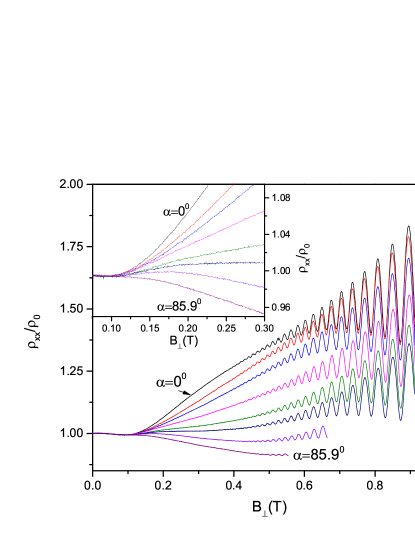
Figure 1: (Color online) Dependence of the longitudinal resistance $\displaystyle\rho_{xx}$ on the magnetic field perpendicular to the 2D sample obtained at different angles $\displaystyle\alpha$ between the total magnetic field $\displaystyle\vec{B}$ and the normal to the 2D layer. From the top curve to the bottom one angles are 0, 76.2, 78.6, 81.2, 82.6 83.13, 84, and 85.9 degrees. The insert enlarges the area at small magnetic fields indicating that the dependencies at different angles diverge from approximately the same magnetic field $\displaystyle B^{*}\approx$0.11T corresponding to the beginning of Landau quantization of the electron spectrum at $\displaystyle\alpha$=0⁰.

Figure 1 presents the dissipative resistivity, $\displaystyle\rho_{xx}(B_{\perp})$, at different angles $\displaystyle\alpha$ between the magnetic field, $\displaystyle\vec{B}$, and the normal to the 2D layer, $\displaystyle\vec{n}$. In perpendicular magnetic fields below 0.11 T the resistance is nearly (within $\displaystyle\sim$0.6%) independent on $\displaystyle B_{\perp}$. This is the regime of classical (Drude) magnetoresistance, which is expected to be independent on $\displaystyle B_{\perp}$.²⁴

At $\displaystyle\alpha=0^{0}$ and $\displaystyle B_{\perp}>$0.11 T the magnetoresistance demonstrates a steep (exponential in $\displaystyle 1/B_{\perp}$) monotonic increase combined with SdH oscillations in $\displaystyle B_{\perp}>$ 0.45 T. This increase is attributed¹⁸ to the quantum positive magnetoresistance (QPMR) due to Landau quantization.²⁵ At angles $\displaystyle\alpha<$ 65^o and $\displaystyle B_{\perp}>$0.33 T the magnetoresistance exhibits an additional few percent increase with the angle (not shown). At $\displaystyle\alpha>$65⁰ the QPMR decreases significantly with the angle. Figure 1 demonstrates this decrease for angles between 76.2 and 85.9 degrees. The insert to the figure shows that the angular variation of QPMR are approximately uniform with $\displaystyle B_{\perp}$ and starts at the $\displaystyle same$ perpendicular magnetic field $\displaystyle B^{*}\approx$0.11 T, which separates the classical and quantum regimes of electron transport^{25; 18}. The later indicates that the Landau level width (or the quantum scattering time $\displaystyle\tau_{q}$) is nearly independent of angle $\displaystyle\alpha$. This is confirmed by more detailed comparison (see Fig.3(d)). At angles $\displaystyle\alpha>$86⁰ the QPMR demonstrates a weak recovery (not shown), which is discussed later.

At $\displaystyle B_{\perp}>$0.45T Fig.1 shows SdH oscillations. In contrast to QPMR the angular evolution of SdH oscillations have been intensively studied.^{7; 8; 10} Presented experiments show $\displaystyle strong$ correlation between angular evolutions of SdH oscillations and QPMR. Before the detail discussion and comparison of the dependencies, we present a model, which captures the strong angular correlations of these two phenomena.

III.1 Model of SdH oscillations and Quantum Positive Magnetoresistance

A microscopic description of both SdH oscillations and QPMR in perpendicular magnetic fields (at $\displaystyle\alpha=$0^o) is presented in paper Ref.[²⁵] neglecting any spin related effects in particular the Zeeman term. As indicated in the ”Introduction” the account of the Zeeman splitting for SdH oscillations is a developed procedure^{6; 3; 8}. In contrast the spin related effects in the QPMR have not been studied yet.

Below we present a model, which utilizes the similarity of QPMR and Magneto-InterSubband (MISO) resistance oscillations.^{26; 27; 28; 29; 30} The model considers two subbands with the energy spectrum evolving in accordance with Landau quantization and splitted predominantly by Zeeman effect.⁶ A scattering assisted mixing between different subbands is $\displaystyle postulated$ to provide the observed correlation between the angular evolutions of SdH oscillations and QPMR. Within the presented model the absence of the scattering between subbands would lead to the absence of an angular evolution of the QPMR associated with the Zeeman effect in contrast to the angular dependence of SdH oscillations. The origin of the mixing requires further investigations. A mixing between different spin subbands have been reported in Si-MOSFETs.³¹ The experiments show a sizable contributions of the product the spin-up and spin-down density of states to SdH resistance oscillations. Furthermore investigations of the resistivity tensor in tilted magnetic fields have revealed an independence of the Hall coefficient on the spin subband populations while the electron mobility in each spin subband was substantially affected by the in-plane magnetic field³². This behavior has been interpreted by a mixing between spin subbands due to an electron-electron interaction.³³ We note also that in the presence of a spin-orbit coupling, different subbands could be mixed by a local impurity scattering. An investigation of this possibility is presented in the section ”Spin orbit interaction and QPMR”.

In the simplest case of small quantizing magnetic fields $\displaystyle\omega_{c}\tau_{q}<1$ the main contribution to both SdH oscillation and QPMR comes from the fundamental harmonic of quantum oscillations of the density of states (DOS) corresponding to spin-up and spin-down subbands. The total DOS, $\displaystyle\nu(\epsilon)$, reads³:

$$\begin{split}\nu(\epsilon)\!&=\!\nu_{0}\!\left[\!1\!-\!\delta cos\!\left(\!\frac{2\pi(\epsilon\!-\!\Delta_{Z}/2)}{\hbar\omega_{c}}\!\right)\!-\!\delta cos\!\left(\!\frac{2\pi(\epsilon\!+\!\Delta_{Z}/2)}{\hbar\omega_{c}}\!\right)\!\right]\\ &=\nu_{0}\left[1-2\delta cos\left(\frac{2\pi\epsilon}{\hbar\omega_{c}}\right)cos\left(\frac{\pi\Delta_{Z}}{\hbar\omega_{c}}\right)\right]\end{split}$$ (2)

where $\displaystyle\delta=exp(-\pi/\omega_{c}\tau_{q})$ is Dingle factor, $\displaystyle\nu_{0}$ is the total DOS at zero magnetic field and $\displaystyle\tau_{q}$ is the quantum scattering time, which is considered to be the same in both spin subbands.

The 2D conductivity $\displaystyle\sigma$ is obtained from the following relation:

$$\sigma(B)=\int d\epsilon\sigma(\epsilon)\left(-\frac{\partial f}{\partial\epsilon}\right)=\langle\sigma(\epsilon)\rangle$$ (3)

The integral is an average of the conductivity $\displaystyle\sigma(\epsilon)$ taken essentially for energies $\displaystyle\epsilon$ inside the temperature interval $\displaystyle kT$ near Fermi energy, where $\displaystyle f(\epsilon)$ is the electron distribution function at the temperature $\displaystyle T$. ³ The brackets represent this integral below.

The following expression approximates the conductivity $\displaystyle\sigma(\epsilon)$ at small quantizing magnetic fields:

$$\sigma(\epsilon,B_{\perp},\Delta_{Z})=\sigma_{D}(B_{\perp})\tilde{\nu}(\epsilon,B_{\perp},\Delta_{Z})^{2}$$ (4)

where $\displaystyle\sigma_{D}(B_{\perp})$ is Drude conductivity in magnetic field $\displaystyle B_{\perp}$ ²⁴ and $\displaystyle\tilde{\nu}(\epsilon)=\nu(\epsilon)/\nu_{0}$ is normalized total density of states. The main assumption of this model is utilized in Eq.(4). Namely the impurity scattering between the spin-up and spin-down subbands is considered to be comparable with the impurity scattering within a spin subband, when the energies of the spin sectors are the same. In other words a spin up (spin-down) electron has equal probability to scatter into a spin-up or spin-down quantum state.

The proportionality of the conductivity $\displaystyle\sigma(\epsilon)$ to the square of the normalized density of states is due to two factors. One factor takes into account the number of available conducting states (parallel channels) at energy $\displaystyle\epsilon$, which is proportional to the density of states. The second factor takes into account that the dissipative conductivity in crossed electric and magnetic fields is proportional to the electron scattering rate²⁴. At low temperatures the scattering is dominated by the elastic impurities making the rate proportional to the density of final states at the same energy $\displaystyle\epsilon$.^{24; 34} The quadratic dependence of the conductivity on the density of state results in the factor 4 in Eq.(5), which is found to be in good quantitative agreement with the amplitude of SdH oscillations shown in Fig.2. Furthermore the quadratic dependence on the density of states yields both QPMR and its strong correlation with SdH oscillations observed in presented experiments.

The Eq.(4) is similar to the Eq.(5) of Ref.[35], which was used for the conductivity in the perpendicular magnetic fields neglecting both the Zeeman splitting and spin-orbital effects. In this case the energy spectrum of spin-up and spin-down electrons are the same and the normalized DOS for each spin subband coincides with the normalized total DOS, $\displaystyle\tilde{\nu}(\epsilon)$. For two independent spin subbands the total conductivity is the sum of two terms: $\displaystyle\sigma_{ind}=\sigma^{+}+\sigma^{-}$, where $\displaystyle\sigma^{\pm}=(\sigma_{D}/2)\tilde{\nu}(\epsilon)^{2}$. The factor $\displaystyle 1/2$ takes into account that the electron density in each subbands is half the total density. Thus at $\displaystyle\Delta_{Z}$=0 the total conductivity of two subbands does not depend on the intersubband scattering: $\displaystyle\sigma_{ind}=\sigma(\Delta_{Z}=0)$. At finite $\displaystyle\Delta_{Z}$ the intersubband scattering affects the conductivity.

A substitution of Eq.(4) and Eq.(2) into Eq.(3) yields two additional terms to the Drude conductivity: $\displaystyle\sigma-\sigma_{D}=\Delta\sigma_{SdH}+\Delta\sigma_{QPMR}$. The first term is proportional to Dingle factor $\displaystyle\delta$ and describes SdH oscillations. It reads:

$$\begin{split}\frac{\Delta\sigma_{SdH}}{\sigma_{D}}&=-4\delta\langle\cos\left(\frac{2\pi\epsilon}{\hbar\omega_{c}}\right)\rangle\cos\left(\frac{\pi\Delta_{Z}}{\hbar\omega_{c}}\right)\\ &=-4\delta A(T)\cos\left(\frac{2\pi\epsilon_{F}}{\hbar\omega_{c}}\right)\cos\left(\frac{\pi\Delta_{Z}}{\hbar\omega_{c}}\right),\end{split}$$ (5)

where $\displaystyle\epsilon_{F}$ is Fermi energy and $\displaystyle A(T)=\frac{(2\pi^{2}kT/\hbar\omega_{c})}{\sinh(2\pi^{2}kT/\hbar\omega_{c})}$ is SdH temperature factor.¹

The second term is proportional to the square of the Dingle factor and describes variations of the conductivity due to QPMR. It reads:

$$\begin{split}\frac{\Delta\sigma_{QPMR}}{\sigma_{D}}&=4\delta^{2}\langle\cos^{2}\left(\frac{2\pi\epsilon}{\hbar\omega_{c}}\right)\rangle\cos^{2}\left(\frac{\pi\Delta_{Z}}{\hbar\omega_{c}}\right)\\ &=\delta^{2}\left[1+\cos\left(\frac{2\pi\Delta_{Z}}{\hbar\omega_{c}}\right)\right],\end{split}$$ (6)

In Eq.(6) the exponentially small temperature dependent term is neglected. At $\displaystyle\Delta_{Z}$=0 Eq.(6) reproduces QPMR in perpendicular magnetic fields.^{25; 18}

Eq.(5) and Eq.(6) indicate the strong angular correlation between the amplitude of SdH oscillations and the QPMR. In particular the SdH amplitude is proportional to $\displaystyle\cos(\pi\Delta_{Z}/\hbar\omega_{c})$ and is zero at $\displaystyle\Delta_{Z}=\hbar\omega_{c}/2$ in agreement with Eq.(1), while the QPMR is proportional to (1+$\displaystyle\cos(2\pi\Delta_{Z}/\hbar\omega_{c})$ and is zero too at $\displaystyle\Delta_{Z}=\hbar\omega_{c}/2$. In the next sections we compare experimental results with Eq.(5) and Eq.(6).

III.2 Shubnikov de Haas oscillations

In quantizing magnetic fields $\displaystyle\omega_{c}\tau_{tr}\gg$1, where $\displaystyle\tau_{tr}$ is the transport scattering time. At this condition resistivity is $\displaystyle\rho_{xx}=\sigma[\rho_{xy}]^{2}$ and $\displaystyle\rho_{xx}(B_{\perp})/\rho_{0}=\sigma(B_{\perp})/\sigma_{D}(B_{\perp})$, where $\displaystyle\rho_{0}$ is Drude resistivity.²⁴ Therefore in accordance with Eq.(5) the amplitude of SdH oscillations of the normalized resistivity, $\displaystyle\Delta\rho_{SdH}/\rho_{0}$, is $\displaystyle A_{SdH}=4\delta A(T)\cos(\pi\Delta_{Z}/\hbar\omega_{c})$ and the normalized SdH amplitude is $\displaystyle A_{SdH}^{norm}=A_{SdH}/(4\delta A(T))=\cos(\pi\Delta_{Z}/\hbar\omega_{c})$. To extract the normalized amplitude $\displaystyle A_{SdH}^{norm}$, the SdH resistance oscillations shown in Fig.1 were separated from the monotonic background using a low frequency filtering.³⁰ The separated SdH oscillations were then divided by the factor $\displaystyle 4\rho_{0}\delta(B_{\perp},\tau_{q})A(T)$. By a variation of the quantum scattering time $\displaystyle\tau_{q}$ in the Dingle factor $\displaystyle\delta$ quantum oscillations with the amplitude, $\displaystyle A_{SdH}^{norm}$, independent on the magnetic field, $\displaystyle B_{\perp}$, are obtained. The later indicates that the ratio of the Zeeman energy, $\displaystyle\Delta_{Z}$ to the cyclotron energy, $\displaystyle\Delta_{C}=\hbar\omega_{c}$ is a constant at fixed angle $\displaystyle\alpha$ in the SdH regime. The insert to Fig.2 shows the independence of the normalized SdH amplitude, $\displaystyle A_{SdH}^{norm}$, on the reciprocal magnetic fields at different angles $\displaystyle\alpha$.

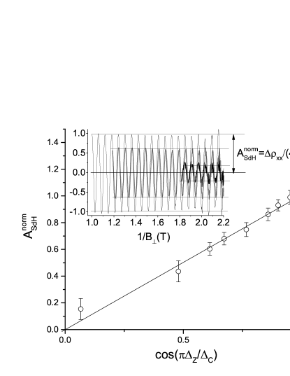
Figure 2: Dependence of normalized amplitude of SdH oscillations, $\displaystyle A_{SdH}^{norm}=A_{SdH}/4\delta A(T)$ on $\displaystyle\cos(\pi\Delta_{Z}/\Delta_{C})$ with $\displaystyle g$=0.97. The dependence corresponds to Eq.(5) relating the angular evolution of SdH amplitude to the angular variation of the ratio between Zeeman and cyclotron energies: $\displaystyle\Delta_{Z}/\Delta_{C}=mg/(2m_{0}\cos\alpha)$. The insert presents normalized SdH resistance oscillations in reciprocal magnetic fields at angles $\displaystyle\alpha$: 67.6, 83.3 and 85.9 degrees.

Figure 2 presents the angular dependence of the normalized SdH amplitude $\displaystyle A_{SdH}^{norm}$. We note that the value of the SdH amplitude agrees quantitatively with the one expected from Eq.(5). The dependence is plotted versus $\displaystyle\cos(\pi\Delta_{Z}/\hbar\omega_{c})=\cos(\pi mg/(2m_{0}\cos\alpha))$. The g-factor is used as a scaling parameter for $\displaystyle x$-axes of the plot to provide the linear dependence between $\displaystyle A_{SdH}^{norm}$ and $\displaystyle\cos(\pi\Delta_{Z}/\hbar\omega_{c})$. The obtained value of g-factor $\displaystyle g$=0.97$\displaystyle\pm$0.08 corresponds to the critical angle $\displaystyle\alpha_{c}$=86.3${}^{o}\pm$0.3^o (see Eq.(1)) and is in a good agreement with existing experiments.^{7; 8; 9; 10} Thus the angular evolution of SdH oscillations agrees with both Eq.(5) and existing experiments. We note that the strong enhancement of the g-factor obtained in the present experiments in the high temperature regime is intriguing, since the enhancement should degrade with temperature increase in the low temperature domain.⁸

The obtained quantum scattering rate, $\displaystyle 1/\tau_{q}$, is presented in Fig.3(d). The scattering rate is found to be independent on the angle $\displaystyle\alpha$: $\displaystyle 1/\tau_{q}^{SdH}\approx 300\pm 100$GHz and agrees with the one obtained using the QPMR described in next section.

III.3 Quantum Positive Magnetoresistance.

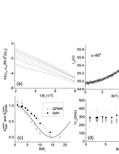
Figure 3: (a) Dependence of the difference between normalized resistivity at an angle $\displaystyle\alpha$ and the normalized resistivity at $\displaystyle\alpha$=85.9⁰$\displaystyle\approx$$\displaystyle\alpha_{c}$: $\displaystyle[\rho_{xx}-\rho_{xx}(85.9^{0})]/\rho_{0}$ on the reciprocal magnetic field. From the top curve to the bottom one corresponding angles $\displaystyle\alpha$ are 70.1, 76.2, 78.6, 81.2, 82.6, 83.3 and 84.3 degrees; (b) magnetoresistance at $\displaystyle\alpha$=90⁰; (c) Dependence of the normalized QPMR and SdH amplitudes on the ratio between total and perpendicular magnetic fields. The solid (dotted) line presents the normalized QPMR (SdH) amplitude: $\displaystyle A_{QPMR}^{norm}=(1+cos(2\pi\Delta_{Z}/\hbar\omega_{c}))/2$ ($\displaystyle A_{SdH}^{norm}$) obtained from Eq.(6) (Eq.(5)) using g-factor $\displaystyle g$=0.97; (d) Dependence of the quantum scattering rate on the ratio $\displaystyle B/B_{\perp}$ obtained from the analysis SdH oscillations and the exponential decrease of the QPMR magnitude with $\displaystyle 1/B_{\perp}$ expected from Eq.(6).

In accordance with Eq.(6) the magnitude of the quantum magnetoresistance decreases exponentially with the reciprocal magnetic field, $\displaystyle 1/B_{\perp}$, due to the exponential decrease of Dingle factor $\displaystyle\delta$. Below we explore this property of the QPMR to extract the quantum scattering rate $\displaystyle 1/\tau_{q}$ and the normalized QPMR amplitude $\displaystyle A_{QPMR}^{norm}=(1+\cos(2\pi\Delta_{Z}/\Delta_{c}))/2$. In the vicinity of the critical angle $\displaystyle\alpha_{c}$ the magnitude of the QPMR is expected to be very small and the magnetoresistance should be mostly driven by other mechanisms.^{36; 37; 38} In particular Fig.3(b) presents the magnetoresistance at angle $\displaystyle\alpha$=90⁰ at which only in-plane magnetic fields is applied. The resistance demonstrates a weak (within 2%) parabolic increase with the in-plane magnetic field. The small in-plane magnetoresistance affects weakly the curves presented in Fig.1 and can be taken into account assuming its independence on the angle $\displaystyle\alpha$. Below we assume that all mechanisms leading to negative magnetoresistance in the vicinity of the critical angle are independent on the angle $\displaystyle\alpha$ and controlled by $\displaystyle B_{\perp}$ and $\displaystyle B_{\parallel}$ independently.

Within this assumption the difference between magnetoresistance at an angle $\displaystyle\alpha$ and the magnetoresistance at the critical angle $\displaystyle\alpha_{c}$ captures the main effect of the angular variations of the electron spectrum on the electron transport described by Eq.(6). Figure 3(a) presents the dependence of the difference between the resistivity $\displaystyle\rho_{xx}(\alpha)$ and $\displaystyle\rho_{xx}(85.9^{0}\approx\alpha_{c})$ normalized to the Drude resistivity $\displaystyle\rho_{0}$ on the reciprocal magnetic field, $\displaystyle 1/B_{\perp}$ taken at different angles. At small magnetic fields, $\displaystyle B_{\perp}$, the dependences demonstrate an exponential decrease with $\displaystyle 1/B_{\perp}$ in accord with Eq.(6) with the rate depending weakly on $\displaystyle\alpha$. With an increase of the angle $\displaystyle\alpha$ the dependencies shift down indicating a decrease of the normalized QPMR amplitude $\displaystyle A_{QPMR}^{norm}$. The presented resistance difference takes into account the small variations of the resistivity with the in-plane magnetic field shown in Fig.3(b). The applied correction to the resistivity affect very weakly (within the size of the symbols) the results presented in Fig.3(c,d).

Fig.3(c) presents the normalized QPMR amplitude $\displaystyle A_{QPMR}^{norm}$ and SdH amplitude $\displaystyle A_{SdH}^{norm}$ plotted vs $\displaystyle 1/\cos\alpha=B/B_{\perp}$. The normalized QPMR amplitude is obtained by the extrapolation of the linear dependencies shown in Fig.3(a) at high $\displaystyle 1/B_{\perp}$ to the infinite $\displaystyle B_{\perp}$. The extracted normalized amplitude $\displaystyle A_{QPMR}^{norm}$ is presented by the open symbols. The solid line shows the amplitude $\displaystyle A_{QPMR}^{norm}$ obtained from Eq.(6) using g-factor $\displaystyle g$=0.97. We note that there are no fitting parameters between the experiment (open symbols) and the Eq.(6) since the g-factor is obtained from the fitting of the angular dependence of the SdH amplitude. Shown in Fig.3(c) comparison of two amplitudes indicates strong angular correlations between SdH resistance oscillations and the quantum positive magnetoresistance.

Fig.3(d) presents the quantum scattering rates obtained from the analysis of SdH resistance oscillations (filled symbols) and QPMR (open symbols). In contrast to SdH resistance oscillations the analysis of the QPMR magnitude yields more accurate results for $\displaystyle\tau_{q}$ since QPMR does not depend on the temperature damping factor $\displaystyle A(T)$ and the response is mostly controlled by the Dingle factor only. The quantum scattering rates extracted by two different methods are found to be in a reasonable agreement indicating no significant variations of the electron lifetime $\displaystyle\tau_{q}$ with both the angle $\displaystyle\alpha$ and the applied magnetic fields at $\displaystyle\alpha<\alpha_{c}$.

Figures 1 and 3(a) demonstrate the evolution of the QPMR, which is obtained at a fixed angle $\displaystyle\alpha$. At this condition both perpendicular and total magnetic fields are changing. As mentioned above the angular evolution of QPMR at small ($\displaystyle<$65⁰) and large ($\displaystyle>\alpha_{c}$) angles demonstrates additional features, which may required a modification of the proposed description. To get further insight into the angular evolution of the QPMR, we have conducted measurements at a fixed perpendicular magnetic field, $\displaystyle B_{\perp}$, while sweeping the in-plane magnetic field, $\displaystyle B_{\parallel}$. At this condition the cyclotron energy is fixed and variations of the electron spectrum are related mostly to spin degrees of freedom.

Figure 4(a) presents dependencies of the normalized resistivity on the total magnetic field taken at the fixed $\displaystyle B_{\perp}$ as labeled. In the agreement with the angular evolution shown in Fig.1 the total magnetic field suppresses the quantum magnetoresistance at a fixed $\displaystyle B_{\perp}$. A stronger perpendicular magnetic field, $\displaystyle B_{\perp}$, requires a stronger total magnetic field, $\displaystyle B$, to suppress the QPMR. After the suppression the magnetoresistance demonstrates a weak increase with the magnetic field, which is, however, much smaller than expected from Eq.(6). Finally at $\displaystyle B_{\perp}>$0.3 T the magnetoresistance shows a maximum enhancing at higher $\displaystyle B_{\perp}$ that is also not explained by this model. The insert to Fig.4(a) presents the position of the resistance maximum at different $\displaystyle B_{\perp}$ indicating that the maximum occurs at $\displaystyle\alpha_{0}\approx$62⁰.

Figure 4(b) presents the magnetic field dependencies of a normalized resistance variation: $\displaystyle\Delta\rho_{xx}/\Delta\rho_{N}=(\rho_{xx}-\rho_{min})/(\rho_{max}-\rho_{min})$, where $\displaystyle\rho_{max}$ and $\displaystyle\rho_{min}$ are maximum and minimum values of the curves shown in (a). The figure facilitates the comparison of the shape of the dependencies at different $\displaystyle B_{\perp}$.

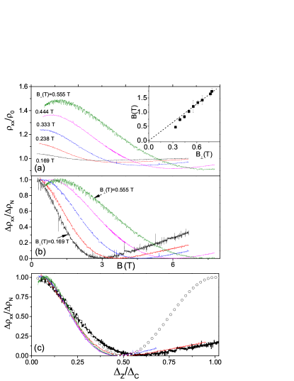
Figure 4: (Color online) (a) Dependence of normalized resistivity on magnetic field at fixed $\displaystyle B_{\perp}$ as labeled. Insert shows position of the resistance maximum at different $\displaystyle B_{\perp}$; (b) Normalized variations of the resistivity shown in (a): $\displaystyle\Delta\rho_{xx}/\Delta\rho_{N}=(\rho_{xx}-\rho_{min})/(\rho_{max}-\rho_{min})$ vs $\displaystyle B$; (c) Normalized variations of the resistivity vs ratio of Zeeman and cyclotron energies, $\displaystyle\mu gB/\hbar\omega_{c}$, with g-factor $\displaystyle g$=0.97 obtained from the angular variation of SdH oscillations. Open symbols present the normalized magnetoresistance expected from Eq.(6) with no fitting parameters.

In accordance with the proposed model (see Eq.(6)) at a fixed $\displaystyle B_{\perp}$ and a constant quantum lifetime $\displaystyle\tau_{q}$ the Dingle factor is fixed and the evolution of the magnetoresistance is solely due to variations of the QPMR amplitude, $\displaystyle A_{QPMR}^{norm}=(1+cos(2\pi\Delta_{Z}/\hbar\omega_{c}))/2$. If the g-factor is also a constant, then the Zeeman term, $\displaystyle\Delta_{Z}=\mu gB$, is linearly proportional to the total magnetic field, $\displaystyle B$, and the QPMR amplitude depends only on the ratio $\displaystyle B/B_{\perp}$. Thus in this case the QPMR should scale with $\displaystyle B/B_{\perp}$.

Figure 4(c) presents the normalized resistance variations, $\displaystyle\Delta\rho_{xx}/\Delta\rho_{N}$, shown in Fig.4(b) plotted against the ratio between Zeeman and cyclotron energies: $\displaystyle\Delta_{Z}/\Delta_{C}=(mg/2m_{0})(B/B_{\perp})$, using the constant g-factor $\displaystyle g$=0.97 obtained from the angular dependence of the amplitude of SdH oscillations. Except the curve taken at the smallest $\displaystyle B_{\perp}$=0.169 T all other curves shown in Fig.4(a,b) collapse on a single dependence at $\displaystyle\Delta_{Z}/\Delta_{C}$ between 0.07 and 0.5. The collapse indicates $\displaystyle B/B_{\perp}$ scaling, which holds at high $\displaystyle B_{\perp}$ in the studied system.

At $\displaystyle\Delta_{Z}/\Delta_{C}<$ 1/2 the scaled dependencies are quite close to the dependence expected from Eq.(6) and presented by the open circles at $\displaystyle g$=0.97 in Fig.4(c) with no fitting parameters. The dependence obtained at the smallest $\displaystyle B_{\perp}$=0.169 T agrees better with the model. We note that the model takes into account only fundamental harmonics of the electron spectrum and, thus, is valid only for overlapping Landau levels at $\displaystyle\omega_{c}\tau_{q}<$1. At $\displaystyle B_{\perp}>$0.3T the Landau levels become separated at $\displaystyle\tau_{q}\approx$4 ps and an account of the higher harmonics of DOS may improve the agreement with the experiment at high $\displaystyle B_{\perp}$. In contrast the description of SdH oscillations is valid even at higher $\displaystyle B_{\perp}$ since the contributions of the higher harmonics of DOS to the SdH amplitude are suppressed by the temperature for presented $\displaystyle B_{\perp}$.^{1; 25} We note also that the shift of the resistive variation at $\displaystyle B_{\perp}$=0.169T to a stronger $\displaystyle B$ ($\displaystyle\Delta_{Z}$) in Fig.4(c) agrees with the reduction of the enhanced g-factor by the disorder ^{17; 8}

An unexpected feature of the dependences presented in Fig.4 is the resistance maximum emerging at high $\displaystyle B_{\perp}$. In accordance with Eq.(6) the maximum occurs at $\displaystyle\Delta_{Z}$=0 and corresponds to the alignment of the quantum levels corresponding to spin-up and spin-down subbands. The presence of the maximum at a finite magnetic field, $\displaystyle B$, suggests that the magnitude of the Zeeman splitting, $\displaystyle|\Delta_{Z}(B_{\perp})|$, decreases with the increase of the total magnetic field, $\displaystyle B$, at a small $\displaystyle B_{\parallel}$. The decrease of the spin spitting is stronger at larger $\displaystyle B_{\perp}$. The total magnetic field, $\displaystyle B_{max}$, corresponding to the resistance maximum at different $\displaystyle B_{\perp}$ is shown in the insert to Fig.4(a). At high $\displaystyle B_{\perp}$ the $\displaystyle B_{max}$ is proportional to $\displaystyle B_{\perp}$ that corresponds to the angle $\displaystyle\alpha_{0}$=62⁰. The position of the maximum agrees, therefore, with the $\displaystyle B/B_{\perp}$ scaling.

The observed behavior is compatible with the following relation between an effective spin slitting $\displaystyle\Delta_{spin}$ and magnetic fields:

$$\Delta_{spin}=\mu|g|B+\Delta_{\perp},\Delta_{\perp}=\beta\hbar\omega_{c}$$ (7)

where $\displaystyle\beta<$0. The parameter $\displaystyle\Delta_{\perp}$ describes the additional contribution of the perpendicular magnetic field to the spin splitting. At the resistance maximum $\displaystyle\Delta_{spin}$=0 yielding $\displaystyle\beta=-m|g|\cos\alpha_{0}/(2m_{0})\approx-$0.016$\displaystyle|g|$.

The structure of the effective spin splitting in Eq.(7) is similar to the one used for 2D electron systems.^{8; 10} In particular in Eq.(10) of Ref.[8]: $\displaystyle\Delta_{spin}=\mu gB+\gamma\hbar\omega_{c}$ the second term proportional to $\displaystyle B_{\perp}$ is the contribution from electron-electron interaction.^{3; 15} The important difference is, however, that the sign of the second term, $\displaystyle\gamma\hbar\omega_{c}$ is opposite to the sign of the term $\displaystyle\Delta_{\perp}$ in Eq.(7). Furthermore the magnitude of the $\displaystyle\beta$ is an order of magnitude smaller the $\displaystyle\gamma\approx$0.2. The origin of these maxima requires further investigations.

At $\displaystyle\Delta_{Z}/\Delta_{C}>$ 1/2 the angular evolution of the QPMR deviates significantly from the expected behavior. Instead of periodic oscillations with the parameter $\displaystyle\Delta_{Z}/\Delta_{C}$ the resistance demonstrates a weak increase at angles $\displaystyle\alpha>86^{0}$ indicating that the modulation of the density of states with the energy does not evolve as expected from Eq.(6). Accounting for the magnetoresistance due to the in-plane magnetic field (presented in Fig.3(b)) reduces this resistance increase at $\displaystyle\Delta_{Z}/\Delta_{C}>$ 1/2 further (not shown).

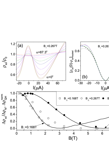
Figure 5: (Color online) (a) Quantal heating of 2D electrons at different angles $\displaystyle\alpha$: 0, 66.4, 76.1,80.8, 83.1, 84.3, 85.4, 86.6, 87.3 deg. at $\displaystyle B_{\perp}$=0.267T; (b) Solid lines are variations of the resistance shown in (a), scaled vertically by factor $\displaystyle k(\alpha)$, vs the electric current $\displaystyle I$ at several angles $\displaystyle\alpha$=0, 76.1, 80.8 and 84.3. Dashed line presents fit, which follows from Eq.(8) for the differential resistance³⁹; (c) Solid curves present smoothed dependencies of the normalized variations of the resistance $\displaystyle\Delta\rho_{xx}/\Delta\rho_{N}$ on the magnetic field $\displaystyle B$. Symbols present the normalized magnitude of the heating induced resistance variation, $\displaystyle\Delta_{QH}^{norm}=k(\alpha)/k_{max}$, obtained at different magnetic fields $\displaystyle B_{\perp}$ and $\displaystyle B$ as labeled.

To get a better understanding of the DOS at $\displaystyle\Delta_{Z}/\Delta_{C}>$ 1/2 we have conducted measurements of quantal heating. ^{19; 20; 21} Figure 5(a) presents dependencies of the normalized differential resistance on the electric current obtained at fixed $\displaystyle B_{\perp}$ and different total magnetic fields $\displaystyle B=B_{\perp}/\cos\alpha$. An application of dc current decreases considerably the differential resistance due to quantal heating. In accordance with theory the magnitude of the heating induced variation of the conductivity at small perpendicular magnetic fields is proportional to the square of the magnitude of DOS modulations with the energy: $\displaystyle 2\delta^{2}$.³⁵ Using Eq.(2) for the DOS and Eq.(4) for the conductivity one can find the effect of quantal heating on the conductivity in a tilted magnetic field following the case corresponding to $\displaystyle\alpha$=0⁰ and considering the inelastic relaxation in the $\displaystyle\tau$-approximation.³⁵ The variation of the conductivity due to quantal heating, $\displaystyle\Delta\sigma_{QH}=\sigma(I)-\sigma(0)$, at $\displaystyle\omega_{c}\tau_{q}<$1 is the following:

$$\frac{\Delta\sigma_{QH}}{\sigma_{D}}=-\delta^{2}\left[1+\cos\left(\frac{2\pi\Delta_{Z}}{\hbar\omega_{c}}\right)\right]\frac{4Q_{dc}}{1+Q_{dc}}.$$ (8)

The term $\displaystyle Q_{dc}=[2\tau_{in}/\tau_{tr}][eER_{c}]^{2}[\pi/\omega_{c}]^{2}$, where $\displaystyle\tau_{in}$ ($\displaystyle\tau_{tr}$) is inelastic (transport) time, $\displaystyle R_{c}$ is cyclotron radius and $\displaystyle E\sim I$ is the electric (Hall) field.^{35; 39} Eq.(8) follows from Eq.(15) of Ref.[35] if one substitutes the factor $\displaystyle 2\delta^{2}$ by $\displaystyle\delta^{2}(1+cos(2\pi\Delta_{Z}/(\hbar\omega_{c}))$. Eq.(8) indicates that the magnitude of the conductivity variation at different angles depends on the factor $\displaystyle[1+\cos(2\pi\Delta_{Z}/(\hbar\omega_{c})]$, which is identical to the one describing QPMR magnitude (see Eq.(6)). On the other hand the factor, $\displaystyle Q_{dc}/(1+Q_{dc})$, describing variations of the resistance with the electric field (current) does not depend on the angle $\displaystyle\alpha$. This means that the shape of the current dependence of the resistance is expected to be the same at different angles, while the overall magnitude of the resistance variations should depend of the angle.

Figure 5(b) demonstrates that the heating induced resistance variations, $\displaystyle\rho_{xx}(0)-\rho_{xx}(I)$, at different angles $\displaystyle\alpha$ are indeed proportional to each other and to the one expected from Eq.(8).³⁹ To reveal the proportionality the curves, shown in Fig.5(a), are scaled vertically to follow the same dependence on the applied current, $\displaystyle I$. At high currents the dependences deviate from the theory due to other mechanisms of nonlinearity.¹⁹

The normalized magnitude of the heating induced resistance variation $\displaystyle\Delta_{QH}^{norm}=k(\alpha)/k_{max}$ are shown in Fig.5(c) at different $\displaystyle B$ and $\displaystyle B_{\perp}$. Here $\displaystyle k(\alpha)$ is the reciprocal scaling coefficients of the curves in Fig.5(b) and $\displaystyle k_{max}$ is the maximum value of $\displaystyle k$. At $\displaystyle\Delta_{Z}/\Delta_{C}<$ 1/2 the heating induced resistance variations follow the QPMR magnitude in agreement with Eq.(6) and Eq.(8) and, thus, correlate with the angular variations of the SdH amplitude. The later is in agreement with previous observations.²¹ At $\displaystyle\Delta_{Z}/\Delta_{C}>$ 1/2 the heating induced resistance variations are absent, indicating the absence of oscillations of the DOS in this regime. On another hand at $\displaystyle\Delta_{Z}/\Delta_{C}<$1/2 the angular evolution of SdH oscillations, QPMR and quantal heating indicates quantization of the electron spectrum demonstrating the electron lifetime, $\displaystyle\tau_{q}\approx$4 ps independent on the angle $\displaystyle\alpha$.

The results show, thus, a rather $\displaystyle abrupt$ transition of the quantized electron spectrum at $\displaystyle\Delta_{Z}/\Delta_{C}<$1/2 to an uniform, energy independent DOS at $\displaystyle\Delta_{Z}/\Delta_{C}>$1/2. Both these results and investigations of the angular evolution of SdH oscillations^{8; 10}, thus, do not support the proposal of a gradual decrease of the quantum scattering time with the in-plane magnetic field.^{40; 41} The observed quenching of MIRO in tilted magnetic fields^{42; 43; 41} also indicates a modification of the electron spectrum, which happens, however, at smaller angles $\displaystyle\alpha<\alpha_{c}$. This suggests that the transition to an energy independent DOS in the high temperature regime, $\displaystyle kT\gg\hbar\omega_{c}$, may depend not only on the ratio between Zeeman and cyclotron energies but also on some other parameters such as electron density, disorder¹⁷ and/or the width of the quantum well.

The angular evolution of QPMR indicates significant spin mixing. This spin mixing suggests an important role of the spin orbit coupling in electron transport at high filling factors. The importance of spin orbit interaction for the quantized spectrum increases at small magnetic fields since the strength of this interaction is independent of magnetic field.^{22; 23} The observed absence of QPMR and quantal heating at $\displaystyle\Delta_{Z}/\Delta_{C}>$1/2 suggests a transition of the quantized electron orbital motion and the independent periodic spin evolution to a stochastic spin-orbital dynamics when energy (period) of the spin evolution is compatible with the energy (period) of the orbital motion. Below we evaluate the effect of spin-orbit interaction on spin mixing in the studied system.

III.4 Spin-Orbit Interaction and Quantum Positive Magnetoresistance.

Spin-orbit coupling in quantum wells and heterojunctions has been discussed in literature⁴. In particular the significant deviation of the g-factor obtained in electrically detected ESR from the bulk GaAs value¹¹ has been attributed to spin-orbit effects.²³ The spin-orbit interaction leads to positive quantum corrections to conductivity of disordered 2D conductors.^{44; 45; 46} In GaAs heterojunctions the effect of spin-orbit interaction on quantum corrections to the conductivity has been investigated.^{47; 48}

We consider that the spin mixing leading to QPMR is due to impurity scattering between different $\displaystyle s$-sectors of the Hamiltonian (9) containing a spin-orbit interaction. To evaluate the spin mixing we first find the electron spectrum, then compute numerically matrix elements of the impurity induced transitions both within an $\displaystyle s$-sector and between different $\displaystyle s$-sectors and compare them.

We consider a 2DEG in the x-y plane placed in a tilted magnetic field and affected by Rashba spin-orbit term. ^{22; 23; 49}. The in-plane component of the magnetic field is chosen to be along the $\displaystyle x$-direction yielding $\displaystyle{\bf B}=(B_{\parallel},0,B_{\perp})$. The Hamiltonian of the system can be written in the following form:

$$\begin{split}H=&\frac{1}{2m}\left({\bf p}+\frac{e}{c}{\bf A}\right)^{2}+\frac{\lambda}{\hbar}\hat{{\bf z}}\cdot\left[\left({\bf p}+\frac{e}{c}{\bf A}\right)\times{\bf\sigma}\right]\\ &+\frac{1}{2}\mu_{B}gB_{\perp}\sigma_{z}+\frac{1}{2}\mu_{B}gB_{\parallel}\sigma_{x}\end{split}$$ (9)

, where $\displaystyle m,-e$ and $\displaystyle\lambda$ are the electron mass, charge and spin-orbit coupling constant, respectively and $\displaystyle\sigma_{i}$ are the Pauli matrices. We employ Landau gauge $\displaystyle\mathbf{A}=-yB\hat{\mathbf{x}}$. In that case the Hamiltonian does not contain $\displaystyle x$ variable and the momentum in $\displaystyle x$-direction $\displaystyle p_{x}=\hbar k$ is a conserved quantity.

As was noted previously ⁴⁹ at angle $\displaystyle\alpha=0$ the problem can be solved analytically yielding the following energy spectrum^{22; 23}

$$E_{n,s}=\hbar\omega_{c}\left(n+\frac{s}{2}\sqrt{(1-g_{s})^{2}+8\eta^{2}n}\right),$$ (10)

where $\displaystyle\eta=\lambda ml_{B}/\hbar^{2}$ and $\displaystyle g_{s}=gm/2m_{0}$. Here $\displaystyle l_{B}=\sqrt{\hbar/eB_{\perp}}$ is the magnetic length. In Eq.(10) $\displaystyle s=1$ for $\displaystyle n=0$ and $\displaystyle s=\pm 1$ for $\displaystyle n>0$. We note that at $\displaystyle\lambda$=2.5 meV$\displaystyle\cdot$nm obtained from an analysis of the ESR spectrum in GaAs heterojunctions^{11; 23} the spin-orbital term, $\displaystyle 8\eta^{2}n$, provides a significant contribution to the gap between different $\displaystyle s$-sectors in Eq.(10) at the high filling factors ($\displaystyle n\sim$30) relevant to the experiments.

The corresponding eigenfunctions have the following form

$$\psi_{n,k,s}(x,y)=\cos\theta_{n,s}\chi_{n,k,+1}+i\sin\theta_{n,s}\chi_{n-1,k,-1}$$ (11)

where $\displaystyle\theta_{0,1}$=0 and for $\displaystyle n>0$, $\displaystyle\tan\theta_{n,s}=-u_{n}+s\sqrt{u_{n}^{2}+1}$ and $\displaystyle u_{n}=(1-g_{s})/(\eta\sqrt{8n})$. Functions $\displaystyle\chi_{n,k,\sigma}=\phi_{n,k}|\sigma\rangle$ present the eigenfunctions of the Hamiltonian (9) at $\displaystyle\lambda=0$ and $\displaystyle B_{\parallel}=0$, where $\displaystyle\phi_{n,k}$ are the Landau level eigenfunctions and $\displaystyle|\sigma\rangle$ is the eigenstate of the spin operator $\displaystyle\sigma_{z}$ with eigenvalues $\displaystyle\sigma=\pm 1$. Each eigenstate $\displaystyle\psi_{n,k,s}$ has the degeneracy $\displaystyle N_{\phi}=L_{x}L_{y}eB/(hc)$ related to $\displaystyle N_{\phi}$ values of $\displaystyle k$, where $\displaystyle L_{x}$ and $\displaystyle L_{y}$ are the system sizes in $\displaystyle x$ and $\displaystyle y$ direction, respectively.

In a tilted magnetic field, $\displaystyle\alpha>0$, the problem can be solved numerically ⁴⁹. An application of the in-plane magnetic field, $\displaystyle B_{\parallel}$, induces transitions between states $\displaystyle\psi_{n,k,s}$ with different index $\displaystyle s$ (between different $\displaystyle s$-sectors). Using functions $\displaystyle\psi_{n,k,s}$ as the basis set, one can present the Hamiltonian in matrix form³⁰. The matrix contains four matrix blocks: $\displaystyle\hat{H}=(\hat{E}^{+},\hat{T};\hat{T}^{*},\hat{E}^{-})$, where the semicolon separates rows. The diagonal matrices $\displaystyle\hat{E}^{+}$ and $\displaystyle\hat{E}^{-}$ represent energy of the $\displaystyle s$-sectors with $\displaystyle s=$1 and $\displaystyle s=$-1, respectively, in different orbital states $\displaystyle n$ following Eq.(10):

$$\begin{split}&E^{+}_{nm}=\delta_{nm}\hbar\omega_{c}\left((n-1)+\frac{1}{2}\sqrt{(1-g_{s})^{2}+8\eta^{2}(n-1)}\right)\\ &E^{-}_{nm}=\delta_{nm}\hbar\omega_{c}\left(n-\frac{1}{2}\sqrt{(1-g_{s})^{2}+8\eta^{2}n}\right)\end{split}$$ (12)

where indexes $\displaystyle n$=1,2…$\displaystyle N_{max}$ and $\displaystyle m$=1,2…$\displaystyle N_{max}$ numerate rows and columns of the matrix correspondingly. In numerical computations the maximum number $\displaystyle N_{max}$ is chosen to be about twice larger than the orbital number $\displaystyle N_{F}$ corresponding to Fermi energy $\displaystyle E_{F}$. Further increase of $\displaystyle N_{max}$ show a very small (within 1%) deviation from the dependencies obtained at $\displaystyle N_{max}\approx 2N_{F}$.

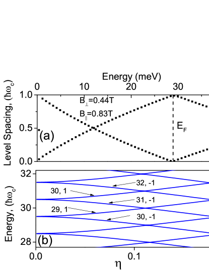
Figure 6: (a) Level spacing $\displaystyle\delta E_{l}=E_{l+1}-E_{l}$ in the energy spectrum of electrons in $\displaystyle B_{\perp}$=0.44 T and $\displaystyle B_{\parallel}$=0.83 T at spin-orbit coupling $\displaystyle\lambda$=2.95 meV$\displaystyle\cdot$nm and $\displaystyle g$=-0.44 . (b) Dependence of the energy of the quantum states in the vicinity of Fermi energy on the spin-orbit coupling parameter $\displaystyle\eta$ at $\displaystyle B_{\perp}$=0.44T and $\displaystyle\alpha$=0⁰. Labels show quantum indexes of the levels according to Eq.(10).

The corresponding matrix elements of the off-diagonal matrix $\displaystyle\hat{T}$ are the following:

$$T_{nm}=i\delta_{nm}\frac{\mu_{B}gB_{\parallel}}{2}\cos\theta_{n-1,1}\sin\theta_{m,-1}$$ (13)

The Hamiltonian $\displaystyle\hat{H}$ is diagonalized numerically at different magnetic fields $\displaystyle B_{\perp}$ and $\displaystyle B_{\parallel}$. To analyze the spectrum the obtained eigenvalues of the Hamiltonian are numerated in ascending order using positive integer index $\displaystyle l$=1,2…. The electron transport depends on the distribution of the quantum levels in the interval $\displaystyle kT$ near the Fermi energy $\displaystyle E_{F}$²⁴. Below we focus on this part of the spectrum.

Figure 6 presents the difference between energies of $\displaystyle l+1$-th and $\displaystyle l$-th quantum levels of the electron spectrum. Each symbol represents a particular level spacing normalized to the cyclotron energy: $\displaystyle\delta E_{l}/\hbar\omega_{c}=(E_{l+1}-E_{l})/\hbar\omega_{c}$.³⁰. Figure 6(a) presents the normalized level spacing at spin-orbit coupling $\displaystyle\lambda$=2.95 meV$\displaystyle\cdot$nm and $\displaystyle g$=-0.44 obtained in $\displaystyle B_{\perp}$=0.44 T and $\displaystyle B_{\parallel}$=0.83 T. These magnetic fields correspond to the QPMR maximum shown in Fig.4. At these conditions the two nearest quantum levels coincide in the vicinity of Fermi energy, $\displaystyle E_{F}$, yielding the level splitting $\displaystyle\Delta^{*}$=0. Fig.6(b) presents the energy of the quantum levels in the vicinity of the Fermi energy vs the strength of the spin-orbit coupling characterized by the coefficient $\displaystyle\eta$ at $\displaystyle B_{\perp}$=0.44 T and $\displaystyle\alpha$=0⁰. Near $\displaystyle\eta\approx$0.11 levels of two different $\displaystyle s$-sectors intersect opening a channel for the impurity scattering between $\displaystyle s$-sectors. Below we evaluate the rate of these transitions for the crossing of the level with quantum numbers $\displaystyle n_{0}$=30, $\displaystyle s$=1 and the one with $\displaystyle n_{0}+2$=32, $\displaystyle s$=-1 and investigate the relation of the scattering matrix elements inside the same $\displaystyle s$-sector and between different $\displaystyle s$-sectors.

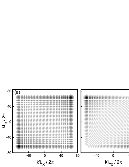
Figure 7: The contour plots of $\displaystyle\left|\langle n_{0},1,k|V(x,y)|n_{0},1,k^{\prime}\rangle\right|$ (a) and $\displaystyle\left|\langle n_{0},1,k|V(x,y)|n_{0}+2,-1,k^{\prime}\rangle\right|$ (b) for different values of $\displaystyle k$ and $\displaystyle k^{\prime}$ for Gaussian impurity potential with parameters $\displaystyle V_{0}=0.1\hbar\omega_{c}$, $\displaystyle a=6.6\cdot 10^{-4}l_{B}$ and $\displaystyle\eta\approx 0.11$.

We approximate the impurity potential by Gaussian function located at $\displaystyle(0,0)$ point:

$$V(x,y)=V_{0}\exp\left[-\frac{x^{2}+y^{2}}{2a^{2}}\right],$$ (14)

where $\displaystyle V_{0}$ is the amplitude of the impurity potential and $\displaystyle a$ defines it’s width. For very narrow impurity potential Eq.(14) can be reduced to a Delta function $\displaystyle V_{D}(x,y)=2\pi V_{0}a^{2}\delta(x)\delta(y)$. In this case at $\displaystyle\alpha$=0⁰ the matrix elements can be written explicitly:

$$\displaystyle\langle n,s,k \displaystyle|V_{D}(x,y)|n^{\prime},s^{\prime},k^{\prime}\rangle=2\pi V_{0}a^{2}\times$$

$$\displaystyle\bigg{[}\sin\theta_{n,s}\sin\theta_{n^{\prime},s^{\prime}}\phi_{n-1,k}(0,0)\phi_{n^{\prime}-1,k^{\prime}}(0,0)+$$

$$\displaystyle\qquad\cos\theta_{n,s}\cos\theta_{n^{\prime},s^{\prime}}\phi_{n,k}(0,0)\phi_{n^{\prime},k^{\prime}}(0,0)\bigg{]},$$ (15)

whereas for general case they should be computed numerically.

Below we compute the matrix elements inside the same $\displaystyle s$-sector $\displaystyle\langle n_{0},1,k|V(x,y)|n_{0},1,k^{\prime}\rangle$ and between different sectors $\displaystyle\langle n_{0},1,k|V(x,y)|n_{0}+2,-1,k^{\prime}\rangle$ at the value $\displaystyle\eta\approx$0.11 and compare the magnitudes of these two matrix elements. In calculations the size of the system in the $\displaystyle y$-direction is $\displaystyle L_{y}=6R_{c}$, where $\displaystyle R_{c}=\sqrt{2n_{0}+1}l_{B}$ is the cyclotron radius.

Fig.7(a) shows a contour plot of the magnitude of the matrix element $\displaystyle\left|\langle n_{0},1,k|V(x,y)|n_{0},1,k^{\prime}\rangle\right|$ within the same $\displaystyle s$-sector while Fig.7(b) shows the magnitude of the impurity scattering between different $\displaystyle s$-sectors $\displaystyle\left|\langle n_{0},1,k|V(x,y)|n_{0}+2,-1,k^{\prime}\rangle\right|$ for different values of $\displaystyle k$ and $\displaystyle k^{\prime}$. The impurity parameters are $\displaystyle V_{0}=0.1\hbar\omega_{c}$ and $\displaystyle a=6.6\cdot 10^{-4}l_{B}$. Fig.7(a) demonstrates that for scattering within the same sector both forward scattering ($\displaystyle k=k^{\prime}$) and backscattering ($\displaystyle k=-k^{\prime}$) are substantial, although forward scattering is somewhat stronger than backscattering. In contrast, in transitions between different $\displaystyle s$-sectors backscattering plays the major role while forward scattering is strongly suppressed. The average of the squares of scattering amplitudes are found to be of the same order: $\displaystyle 1.22\cdot 10^{-19}(\hbar\omega_{c})^{2}$ within the same $\displaystyle s$-sector and $\displaystyle 0.72\cdot 10^{-19}(\hbar\omega_{c})^{2}$ between different $\displaystyle s$-sectors. Thus due to backscattering the impurity scattering between different $\displaystyle s$-sectors is comparable with that within the same $\displaystyle s$-sector. We note that the studied systems demonstrate a significant magnitude of impurity backscattering.^{50; 51; 52}

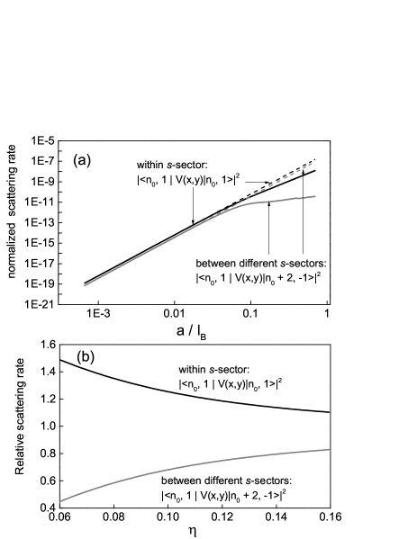
Figure 8: (a) The dependence of the square of matrix elements on impurity width parameter $\displaystyle a$ both for Gaussian $\displaystyle V(x,y)$ and Delta $\displaystyle V_{D}(x,y)$ function potential cases for $\displaystyle\eta\approx 0.11$. (b) The dependence of the square of matrix elements on the value of spin-orbit interaction parameter $\displaystyle\eta$ for Gaussian impurity with the width parameter $\displaystyle a=6.6\cdot 10^{-4}l_{B}$. The impurity amplitude is $\displaystyle V_{0}=0.1\hbar\omega_{c}$ for both figures and the amplitudes of matrix elements are averaged over all $\displaystyle k$ and $\displaystyle k^{\prime}$ values.

Fig.8(a) presents the dependence of the averaged square of the matrix elements on the shape of the impurity potential $\displaystyle V(x,y)$ at $\displaystyle\eta\approx 0.11$. The average is over all $\displaystyle k$ and $\displaystyle k^{\prime}$ values. This figure shows that at $\displaystyle a<0.05l_{B}$ both Gaussian and Delta function potentials provide nearly identical scattering both within the $\displaystyle s$-sector and between different $\displaystyle s$-sectors and the scattering magnitude is proportional to the cross-section of the impurity potential $\displaystyle a^{2}$. At higher magnetic fields $\displaystyle a>0.05l_{B}$ the scattering on the Gaussian potential deviates from the $\displaystyle a^{2}$ dependence. More importantly the figure shows that at $\displaystyle a>0.05l_{B}$ the impurity potential cannot provide significant scattering between different $\displaystyle s$-sectors. Thus the scattering between different $\displaystyle s$-sectors is effective at relatively small magnetic fields (high filling factors) and/or for sharp impurities. At the upper limit of the perpendicular magnetic fields used in this study, $\displaystyle B_{\perp}\approx$1 T, the magnetic length $\displaystyle l_{B}\approx$25 nm and for impurities with size $\displaystyle a$ less 1nm backscattering is effective and leads to the strong spin mixing at $\displaystyle B_{\perp}<$1T. The size, $\displaystyle a<$1 nm, is reasonable for neutral impurities in a solid.

Due to the impurity scattering quantum levels are broadened and the elastic transitions may occur in an interval of the energies when two levels overlap. Thus the scattering may exist in an interval of the parameter $\displaystyle\eta$. Figure 8(b) presents the dependence of the averaged square of matrix elements on the parameter $\displaystyle\eta$. The $\displaystyle\eta$ is varied in the range, where the energy of the system changes by about $\displaystyle 0.6\hbar\omega_{c}$. It accounts, thus, for a significant broadening of quantum levels. The figure shows that the amplitudes of both the intra-sector and inter-sectors scattering are quite comparable in the broad range of $\displaystyle\eta$ and the difference decreases with the $\displaystyle\eta$ increase. The increase of the scattering between different $\displaystyle s$-sectors is related to the fact that at $\displaystyle\eta=0$ different sectors correspond to eigenstates with different $\displaystyle z$ components of the electron spin. These states cannot be coupled by the impurity scattering unless a magnetic impurity is involved (see Eq.(15)). Due to the fact that the majority of the impurities in the studied systems are non-magnetic the scattering between different sectors is completely mediated by the spin-orbit interaction and increases with the increase of the spin-orbit coupling.

The presented estimations of the impurity scattering in the presence of spin-orbit interaction indicate that in the range of physical parameters relevant to presented experiments the scattering between different $\displaystyle s$-sectors is comparable with the scattering within the same $\displaystyle s$-sector. This leads to strong spin mixing in the studied systems and, thus, support the assumption used for Eq.(3).

IV Conclusion

Quantum positive magnetoresistance (QPMR) of 2D electrons is studied at different angles $\displaystyle\alpha$ between the magnetic field and the normal to the 2D layer. The magnitude of QPMR varies significantly with the magnetic field tilt. The angular evolution of QPMR correlate strongly with angular variations of the amplitude of SdH resistance oscillations indicating that the Zeeman spin splitting, $\displaystyle\Delta_{Z}$, enhanced by electron-electron interaction, is the dominant mechanism leading to the QPMR reduction. Surprisingly no quantization of the electron spectrum is detected when the Zeeman energy exceeds the half of the cyclotron energy suggesting a transformation of the electron dynamics in the high temperature regime at $\displaystyle kT\gg\Delta_{Z}>\hbar\omega_{c}/2$ .

In contrast to SdH oscillations the angular evolution of QPMR implies substantial mixing between spin subbands. A spin mixing have been detected in other 2D electrons systems.^{31; 32} Although the origin of the spin mixing remains puzzling investigations indicate, that the spin-orbit interaction may lead to a significant spin mixing via impurity scattering in the studied system.

This work was supported by the National Science Foundation (Division of Material Research - 1104503), the Russian Foundation for Basic Research (Project No. 14-02-01158) and the Ministry of Education and Science of the Russian Federation. We also acknowledge support from NSF EFRI 1542863 (AG) and (PG).

References

- (1) D. Shoenberg Magnetic oscillations in metals, (Cambridge University Press, New York, 1984).
- (2) Sankar D. Sarma, Aron Pinczuk Perspectives in Quantum Hall Effects, (Wiley-VCH, Weinheim, 2004).
- (3) T. Ando, A. B. Fowler, and F. Stern, Rev. of Mod. Phys. B 54, 437 (1982).
- (4) M.I. Dyakonov (Ed.), Spin Physics in Semiconductors, (Springer-Verlag Berlin Heidelberg, 2008).
- (5) A. B. Fowler, F. F. Fang, W. E. Howard, and P. J. Stiles, Phys. Rev. Lett. 16, 901 (1966).
- (6) F. F. Fang, and P. J. Stiles, Phys. Rev. 174, 823 (1968).
- (7) R. J. Nicholas, R. J. Haug, K. v. Klitzing and G. Weimann, Phys. Rev. B 37, 1294 (1988).
- (8) D. R. Leadley, R. J. Nicholas, J. J. Harris and C. T. Foxon, Phys. Rev. B 58, 13036 (1998).
- (9) 4B. A. Piot, D. K. Maude, M. Henini, Z. R. Wasilewski, J. A. Gupta et al., Phys. Rev. B 75, 155332 (2007).
- (10) A. T. Hatke, M. A. Zudov, L. N. Pfeiffer, and K. W. West, Phys. Rev. B 85, 241305(R) (2012).
- (11) D. Stein, K. V. Klitzing, and G. Weimann, Phys. Rev. Lett. 51, 130 (1983).
- (12) Yu. A. Nefyodov, A. V. Shchepetilnikov, I. V. Kukushkin, W. Dietsche, and S. Schmult, Phys. Rev. B 83, 041307(R) (2011).
- (13) A. Usher, R.J. Nicholas, J.J. Harris, and C.T. Foxon, Phys. Rev. B 41, 1129 (1990).
- (14) 15V.T. Dolgopolov, A.A. Shashkin, A.V. Aristov, D. Schmerek, W. Hansen, J.P. Kotthans, and M. Holland, Phys. Rev. Lett. 79, 729 (1997).
- (15) I.L. Aleiner and L.I. Glazman, Phys. Rev. B 52, 11 296 (1995).
- (16) M. A. Paalanen, D. C. Tsui and A. C. Gossard, Phys. Rev. B 25, 5566 (1982); H. P. Wei, S. Y. Lin, D. C. Tsui, and A. M. M. Pruisken, ibid 45, 3926 (1992); G. S. Boebinger, Ph. D. thesis, MIT, 1986; P. T. Coleridge, P. Zawadzki, and A. S. Sachrajda, Phys. Rev. B 49, 10798 (1994); L. P. Rokhinson, B.Su, and V. J. Goldman, Solid State Commun. 96, 309 (1992).
- (17) M. M. Fogler and B. I. Shklovskii, Phys. Rev. B 52, 17366 (1995).
- (18) Scott Dietrich, Sergey Vitkalov, D. V. Dmitriev and A. A. Bykov, Phys. Rev. B 85, 115312 (2012).
- (19) Jing Qiao Zhang, Sergey Vitkalov, and A. A. Bykov Phys. Rev. B 80, 045310 (2009).
- (20) N. C. Mamani, G. M. Gusev, O. E. Raichev, T. E. Lamas, and A. K. Bakarov, Phys. Rev. B 80, 075308 (2009).
- (21) N. Romero, S. McHugh, M. P. Sarachik, S. A. Vitkalov and A. A. Bykov, Phys. Rev. B 78, 153311 (2008).
- (22) E. I. Rashba, Sov. Phys.-Solid State 2, 1109 (1960).
- (23) Yu. A. Bychkov and E. I. Rashba, JETP Lett. 39, 78 (1984).
- (24) J. M. Ziman Principles of the theory of solids, (Cambridge at the University Press, 1972).
- (25) M. G. Vavilov and I. L. Aleiner, Phys. Rev. B 69, 035303 (2004).
- (26) P. T. Coleridge, Semicond. Sci. Technol. 5, 961 (1990).
- (27) D. R. Leadley, R. Fletcher, R. J. Nicholas, F. Tao, C. T. Foxon, and J. J. Harris, Phys. Rev. B 46, 12439 (1992).
- (28) M. E. Raikh, T. V. Shahbazyan, Phys. Rev. B 49, 5531 (1994).
- (29) O. E. Raichev, Phys. Rev. B 78, 125304 (2008).
- (30) William Mayer, Jesse Kanter, Javad Shabani, Sergey Vitkalov, A. K. Bakarov and A. A. Bykov, Phys. Rev. B 93, 115309 (2016).
- (31) Sergey A. Vitkalov, Hairong Zheng, K. M. Mertes, M. P. Sarachik, and T. M. Klapwijk, Phys. Rev. Lett. 85, 2164 (2000). S. A. V. thanks Prof. M. E. Raikh for the indication of the relevance of the observed product of the spin-up and spin-down density of states to a spin inter-subband scattering.
- (32) S. A. Vitkalov, H. Zheng, K. M. Mertes, M. P. Sarachik, and T. M. Klapwijk, Phys. Rev. B 63,193304 (2001).
- (33) Sergey A. Vitkalov, Phys. Rev. B 64, 195336 (2001).
- (34) V. F. Gantmakher, Y. B. Levinson Carrier Scattering in Metals and Semiconductors, (North-Holland, 1987).
- (35) I. A. Dmitriev, M.G. Vavilov, I. L. Aleiner, A. D. Mirlin, and D. G. Polyakov, Phys. Rev. B 71, 115316 (2005).
- (36) E. M. Baskin, L. I. Magarill, and M. V. Entin, Sov. Phys. JETP 48, 365 (1978).
- (37) M. M. Fogler, A. Yu. Dobin, V. I. Perel, and B. I. Shklovskii, Phys. Rev. B 56, 6823 (1997).
- (38) D.G. Polyakov, F. Evers, A. D. Mirlin, and P.Wolfle, Phys. Rev. B 64, 205306 (2001).
- (39) Jing-qiao Zhang, Sergey Vitkalov, A. A. Bykov, A. K. Kalagin, and A. K. Bakarov, Phys. Rev. B 75, 081305(R) (2007).
- (40) A. T. Hatke, M. A. Zudov, L. N. Pfeiffer, and K. W. West, Phys. Rev. B 83, 081301(R) (2011).
- (41) A. Bogan , A. T. Hatke, S. A. Studenikin, A. Sachrajda, M. A. Zudov, L. N. Pfeiffer and K. W. West, Phys.Rev. B 86, 235305 (2012).
- (42) R. G. Mani, Phys. Rev. B 72, 075327 (2005).
- (43) C. L. Yang, R. R. Du, L. N. Pfeiffer, and K. W. West, Phys. Rev. B 74, 045315 (2006).
- (44) S. Hikami, A. I. Larkin, and Y. Nagaoka, Prog. Theor. Phys. 63, 707 (1980).
- (45) S. V. Iordanskii, Yu. B. Lyanda-Geller, and G. E. Pikus, JETP Lett. 60, 206 (1994).
- (46) Yasufumi Araki, Guru Khalsa, and Allan H. MacDonald, Phys. Rev. B 90,125309 (2014).
- (47) T. Hassenkam, S. Pedersen, K. Baklanov, A. Kristensen, C. B. Sorensen, and P. E. Lindelof, F. G. Pikus, and G. E. Pikus, Phys. REv. B 55, 9298 (1997).
- (48) J. B. Miller, D.M. Zumbuhl, C.M. Marcus, Y. B. Lyanda-Geller, D. Goldhaber-Gordon, K. Campman, and A. C. Gossard, Phys. REv. Lett. 90, 076807 (2003).
- (49) Zhan-Feng Jiang, Shun-Qing Shen, and Fu-Chun Zhang, Phys. Rev. B 80, 195301 (2009).
- (50) C. L. Yang, J. Zhang, R. R. Du, J. A. Simmons, and J. L. Reno, Phys. Rev. Lett. 89, 076801 (2002).
- (51) M. G. Vavilov, I. L. Aleiner, and L. I. Glazman, Phys. Rev. B 76, 115331 (2007).
- (52) William Mayer, Sergey Vitkalov and A. A. Bykov, Phys. Rev. B 93, 245436 (2016).