Path counting on simple graphs: from escape to localization

Abstract

We study the asymptotic behavior of the number of paths of length $N$ on several classes of infinite graphs with a single special vertex. This vertex can work as an entropic trap for the path, i.e. under certain conditions the dominant part of long paths become localized in the vicinity of the special point instead of spreading to infinity. We study the conditions for such localization on decorated star graphs, regular trees and regular hyperbolic graphs as a function of the functionality of the special vertex. In all cases the localization occurs for large enough functionality. The particular value of transition point depends on the large-scale topology of the graph. The emergence of localization is supported by the analysis of the spectra of the adjacency matrices of corresponding finite graphs.

I Introduction

In this work we study the asymptotic behavior of the total number of paths of length $N$ on several classes of regular graphs. We call this a ”path counting” (PC) problem as opposed to a more usual ”random walk” problem (RW) which studies the distribution of the end points of symmetric random walks on graphs. The difference between PC and RW is in different normalizations of the elementary step: for PCs all steps enter in the partition function with the weight one, while for symmetric RWs, the step probability depends on the vertex degree, $p$: the probability to move along each graph bond equals $p^{-1}$. For graphs with a fixed vertex degree, the PC partition function and the RW probability distribution differ only by the global normalization constant, and corresponding averages are indistinguishable. However, for inhomogeneous graphs the distinction between PC and RW is crucially: in the path counting problem ”entropic” localization of the paths may occur, while it never happens for random walks. The distinction between PC and RW, and the entropic localization phenomenon were first reported for self-similar structures in 17 and later were rediscovered for star graphs in ternovsky . More recently this phenomenon was studied for regular lattices with defects in burda where authors introduce a notion of “maximal entropy random walk” which is essentially identical to our path-counting problem.

Following ternovsky we begin with star-like discrete graphs, ${\cal G}$, i.e. a union of $p$ discrete half-lines joint together in one point (the root) – see the Fig.1a – just this model was a subject of the work ternovsky . Regard all $N$-step discrete trajectories on ${\cal G}$, and define $Z_{N}(x)$, the total number of trajectories starting from the root of the graph, and ending at distance $x=0,1,2,...$ from the root (regardless on which particular branch the path ends). One can consider $Z_{N}(x)$ as a partition function of an ideal polymer chain with $N$ links with one end fixed in the root of the graph ${\cal G}$ and another end to be anywhere. Given the partition function $Z_{N}(x)$, one can define the corresponding averages:

$$\left<x^{2}(N|p)\right>=\frac{\displaystyle\sum_{x=0}^{\infty}x^{2}Z_{N}(x|p)}{\displaystyle\sum_{x=0}^{\infty}Z_{N}(x|p)}.$$ (1)

The straightforward computations ternovsky show that the asymptotic behavior of $\left<x^{2}(N|p)\right>$ at $N\to\infty$ for large $N$ depends drastically on the number of branches, $p$, in the star-like graph ${\cal G}$. Indeed,

$$\left<x^{2}(N|p)\right>_{N\to\infty}\to f(p)\times\left\{\begin{array}[]{ll}O(N),&\quad p=1,2;\vskip 6.0pt plus 2.0pt minus 2.0pt\\ O(1),&\quad p=3,4,...\end{array}\right.$$ (2)

where $f(p)$ is some positive function which depends on $p$ only and does not depend on $N$. In other words, for $p=1,2$ (the half-line and the full line) the trajectories on average diverge from the origin with the typical distance proportional to $\sqrt{N}$, as one would naturally expect for a regular random walk. Besides, for $p>2$ the trajectories on average stay localized in the vicinity of the junction point.

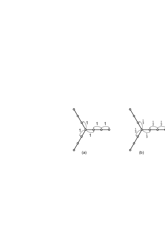
Figure 1: Star-like graph with $p=3$ branches. In a) we enumerate trajectories and each step carries a weight 1. In b) the random-walk the local transition probabilities satisfy conservation condition in each vertex.

To understand qualitatively this behavior, note that the recursion relation connecting $Z_{N}(x|p)$ with $Z_{N+1}(x|p)$ crucially depends on whether $x$ is the root point ($x=0$), or not. Indeed, for each trajectory of length $N$ ending at a point $x\geq 1$ there are exactly two possible ways to add $(N+1)$-th step to it, thus each such path ”gives birth” to two paths of length $(N+1)$. Contrary to that, for each $N$-step path which ends at $x=0$, there are $p$ different ways of adding a new step. Therefore, for $p>2$ passing to $x=0$ becomes entropically favorable, and the root point plays a role of an effective ”entropic trap” for trajectories.

Let us emphasize that this peculiar behavior of the partition function (as a function of $p$) is specific to the path counting problem, and manifests itself in the equilibrium (combinatoric) computations of ideal polymer conformational statistics. Contrary to that, one can think of a closely related non-equilibrium problem, namely calculation of a probability distribution, $P_{N}(x|p)$, for the end-to-end distance of $N$-step random walk on the star graph of $p$ branches. In that case, the probability distribution, due to the normalization condition, should be integrated into 1 on each step, which leads to the obvious normalization of $P_{N}(x,p)$:

$$\sum_{x=0}^{\infty}P_{N}(x|p)=1\;\mbox{for any}\;N.$$ (3)

Therefore, the entropic advantage to stay at the origin is compensated by the fact that possible steps from the origin have probability $p^{-1}$ instead of $1/2$. In other words, if in the path counting problem all trajectories have equal weights 1, in the random walk problem the trajectories have weights $2^{-(N-n)}p^{-n}$, where $n$ is the number of returns to the point $x=0$, varying from a path to path. It is easy to see that in the random walk problem

$$\lim_{N\to\infty}\frac{\left<x^{2}(N|p)\right>}{N}=\lim_{N\to\infty}\frac{1}{N}\sum_{x=0}^{\infty}x^{2}P_{N}(x|p)={\rm const}>0$$ (4)

regardless the value of $p$.

The qualitative arguments supported by exact computations for specific models, demonstrate that entropic localization in the path counting occurs in inhomogeneous systems with broken translational invariance. On uniform trees there is no entropically favorable vertices and PC does not exhibit any localization transitions texier . However, as we see below, the localization is topology-dependent phenomena and occurs on decorated graphs.

The paper is organized as follows. In the Section II we consider finite tree-like regular graphs with a special vertex (“entropic trap”) at the origin, and compute the asymptotics of its partition function based on the spectral properties of the graph adjacency matrix. We show, however, that this approach has some limitations: even increasing the size of the tree to infinity we cannot capture a non-localized solution properly. Indeed, it is not surprising: a finite tree of any size has a non-vanishing fraction of nodes with the degree ”1” (terminal “leaves”). In turn, an infinitely large tree does not have such vertices, and therefore not all of its properties can be recovered by studying the sequence of increasing finite graphs. To resolve this problem in the Section III (which plays the central role in the paper), we study infinite tree-like graphs with a special vertex, and show that depending on the functionality of the vertex, there indeed exists a transition between localized and delocalized state. In the Section IV we generalize the results for two other families of graphs with a special entropically attractive point (we call these two families “decorated star graphs” and “regular hyperbolic graphs”). In the last Section we summarize and discuss the obtained results and formulate some open questions.

II Path counting on finite tree-like graphs

Consider an arbitrary graph $\cal{G}$ with the adjacency matrix $B_{\cal{G}}$. It is easy to see that the partition function $Z_{N}$ described above can be easily expressed in terms of $B_{\cal{G}}$. Indeed, matrix elements of $B_{\cal{G}}^{N}$,

$$\left<i|B_{G}^{N}|j\right>$$ (5)

enumerate walks of length $N$ starting in vertex $j$ and ending in vertex $i$. Therefore, e.g., the total number of paths starting at $i$-th vertex and ending at distance $x$ from it, $Z^{(i)}_{N}(x)$, equals the sum of the matrix elements over all $j$ with a given distance $x$ from $i$

$$Z^{(i)}_{N}(x)=\sum_{j:\text{dist}(i,j)=x}\left<i|B_{G}^{N}|j\right>.$$ (6)

Clearly, this means that asymptotic behavior of $Z_{N}$ is controlled by the largest eigenvalue of $B_{\cal G}$, $\lambda_{\text{max}}({\cal G})$. More precisely, in the large $N$ limit

$$\log Z_{N}(x)\approx N\log\lambda_{\text{max}}({\cal G})+o(N).$$ (7)

Note that for bimodal graphs there always exists a symmetrical pair of largest eigenvalues $\pm\lambda_{\text{max}}(\cal{G})$; as a result $Z_{N}(x)$ alternate between the value prescribed by (7) for even $(N+x)$ and 0 for odd $(N+x)$. In what follows this trivial alternating behavior will appear recurrently and will not be specially mentioned.

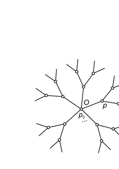
Figure 2: Image of a regular $p$-branching Cayley tree with $p_{0}$ branches at the origin $x=0$. The particular case of a tree with $p=3,n=3$ is shown.

As a particular example of ${\cal G}$, consider a regular branching tree-like graph with $p_{0}$ branches coming out of the origin, and $p$ branches out of any other vertex (as we are interested in a possible localization at the origin, we suppose $p_{0}\geq p$). The maximum number of generations is $n$. The number of vertices in such a graph grows exponentially with $n$, so the direct analysis of its spectrum might seem challenging. However, it turns out that one can drastically simplify the problem by exploiting the symmetries of $\cal G$. Indeed, according to rojo2005 ; rojo2007 the set of eigenvalues of $B_{\cal{G}}$ coincides with the set of eigenvalues of a tri-diagonal symmetric matrix $A_{n}$ with elements $a_{ij}^{(n)}$, which are defined as follows:

$$\begin{cases}a_{i,i}^{(n)}=0\vskip 6.0pt plus 2.0pt minus 2.0pt\\ a_{n,n-1}^{(n)}=a_{n-1,n}^{(n)}=\sqrt{p_{0}}\vskip 6.0pt plus 2.0pt minus 2.0pt\\ a_{i,i-1}^{(n)}=a_{i-1,i}^{(n)}=\sqrt{p-1};\qquad(i=2,...,n-1).\end{cases}$$ (8)

The eigenvalues of $j\times j$ submatrices correspond to multiply degenerated eigenvalues of $B_{\cal{G}}$ (the multiplicity of eigenvalues equals the number of vertices at the generation $n-j$ of the tree from the root point). The corresponding eigenvectors are localized on the outer branches, exactly vanishing at the lowest $n-j$ generations, and take alternating values at the adjacent outer sub-branhces. The eigenvalues of the whole matrix $A_{n}$ are non-degenerate and their eigenvectors span the whole tree. It follows immediately, that the largest eigenvalue of $B_{\cal{G}}$ which is of crucial importance in order to estimate the asymptotics of $Z_{N}$, is an eigenvalue of the matrix $A_{n}$ itself: indeed, its eigenvector should be positively defined. Thus, the study of the spectrum of an exponentially large matrix $B_{\cal{G}}$, is reduced to a similar study of a small and simple matrix $A_{n}$, which can be easy treated both numerically (see the Fig.3) and analytically.

Figure 3: Spectral density of the matrix $A_{1000}$ (a) the localization transition, (b) at the transition point and (c) in the localized phase. Red line indicates $\lambda=p$.

The characteristic polynomial $\mathrm{P}_{n}(p_{0},p)$ for the matrix $A_{n}$ satisfies the recursion relation KovalevaValbaNechaev :

$$\begin{cases}\mathrm{P}_{n}(p_{0},p)=\lambda\mathrm{P}_{n-1}(p_{0},p)-(p-1)\mathrm{P}_{n-2}(p_{0},p);\vskip 6.0pt plus 2.0pt minus 2.0pt\\ \mathrm{P}_{0}(p_{0},p)=\frac{p_{0}}{p-1};\vskip 6.0pt plus 2.0pt minus 2.0pt\\ \mathrm{P}_{1}(p_{0},p)=\lambda.\end{cases}$$ (9)

This system is easy to solve if one looks for $\mathrm{P}_{n}(p_{0},p)$ in the form

$$\mathrm{P}_{n}(p_{0},p)=C_{+}\mu_{+}^{n}+C_{-}\mu_{-}^{n},$$ (10)

giving

$$\mu_{\pm}=\frac{{\lambda}\pm\sqrt{{\lambda}^{2}-4(p-1)}}{2},$$ (11)

and

$$C_{\pm}=\frac{p_{0}}{2(p-1)}\mp\frac{\lambda(p_{0}-2(p-1))}{2(p-1)\sqrt{{\lambda}^{2}-4(p-1)}}.\vskip 6.0pt plus 2.0pt minus 2.0pt$$ (12)

It is easy to see that the resulting equation $\mathrm{P}_{n}(p_{0},p)=0$ is even with respect to $\lambda$. To solve it, define a new variable $\phi$ by

$$\lambda=\pm 2\sqrt{p-1}\cosh{\phi},$$ (13)

where $|\lambda|\geq 2\sqrt{p-1}$ corresponds to real $\phi$ and $\lambda<2\sqrt{p-1}$ – to purely imaginary $\phi$. Then

$$\begin{array}[]{l}\displaystyle\mu_{\pm}=\sqrt{p-1}e^{\pm\phi},\vskip 6.0pt plus 2.0pt minus 2.0pt\\ \displaystyle C_{\pm}=\frac{p_{0}}{2(p-1)}\pm\frac{p_{0}-2(p-1)}{2(p-1)\tanh\phi},\end{array}$$ (14)

and the equation $\mathrm{P}_{n}(p_{0},p)=0$ becomes

$$\tanh n\phi=\frac{p_{0}}{p_{0}-2(p-1)}\tanh\phi,$$ (15)

which for any $n$ has many imaginary solutions and a single real one, which corresponds to $\lambda_{\text{m}ax}^{(n)}$. The limit of this solution for $n\to\infty$ is

$$\lambda_{\max}=\lim_{n\to\infty}\lambda_{\max}^{(n)}=\frac{p_{0}}{\sqrt{p_{0}-p+1}}.$$ (16)

Therefore, we conclude that on any large but finite tree the number of trajectories in the $N\to\infty$ limit behaves asymptotically as (see eq. (7))

$$Z_{N}(x,p,p_{0},n)\sim(\lambda_{\text{m}ax})^{N}=\left(\frac{p_{0}}{\sqrt{p_{0}-p+1}}\right)^{N}.$$ (17)

This result, however, looks a bit strange after close examination: for a partition function on an infinite tree there exists (for $p_{0}\geq p$) a lower bound

$$Z_{N}(x,p,p_{0},n=\infty)\geq p^{N}.$$ (18)

Indeed, on each step there exist at least $p$ different directions to go, which seems to contradict (17) for $p<p_{0}<\bar{p}_{0}=p^{2}-p$. This apparent discrepancy is, of course, due to the order of taking limits $n\to\infty$ and $N\to\infty$. In a system with large but finite $n$ there is always a finite fraction of terminal nodes (“leaves” of the tree) with degree ”1”, violating the reasoning behind (18). In turn, in a system with infinite $n$, as we show in the next Section, there exists an additional eigenvalue of the adjacency matrix equal to $p$, corresponding to a density wave spreading with finite velocity from the root point to infinity. Depending on which of two eigenvalues, the one given by (16), or this new, $\lambda=p$, is maximal, the partition function of the infinitely large system is either localized, or, respectively, delocalized.

III Localization of trajectories on an infinite tree with a ”heavy” root

Consider the same graph ${\cal G}$ as defined above (see Fig.2) but with infinitely large number of generations $n$. We start with writing explicitly the recursion relation for the partition function, $Z_{N}(x)$, of all $N$-step paths on ${\cal G}$, starting at the origin and ending at some distance $x$ from it:

$$\left\{\begin{array}[]{rcll}\displaystyle Z_{N+1}(x)&=&(p-1)Z_{N}(x-1)+Z_{N}(x+1),&\quad x\geq 2\vskip 6.0pt plus 2.0pt minus 2.0pt\\ \displaystyle Z_{N+1}(x)&=&p_{0}Z_{N}(x-1)+Z_{N}(x+1),&\quad x=1\vskip 6.0pt plus 2.0pt minus 2.0pt\\ Z_{N+1}(x)&=&Z_{N}(x+1),&\quad x=0\vskip 6.0pt plus 2.0pt minus 2.0pt\\ Z_{N}(x)&=&0,&\quad x\leq-1\vskip 6.0pt plus 2.0pt minus 2.0pt\\ Z_{N=0}(x)&=&\delta_{x,0},\end{array}\right.$$ (19)

where $x$ is the distance from the root of the Cayley graph ${\cal G}$, measured in number of generations of the tree.

In order to solve this set of equations koleva ; gangardt we make a shift $x\to x+1$, and substitute

$$Z_{N}(x)=A^{N}B^{x}W_{N}(x).$$ (20)

with $A=B=\sqrt{p-1}$. This substitution allows to symmetrize the original equation, which in terms of $W$ takes now the form

$$\left\{\begin{array}[]{rcll}W_{N+1}(x)&=&\displaystyle W_{N}(x-1)+W_{N}(x+1)+\frac{p_{0}-p+1}{p-1}\,\delta_{x,2}\,W_{N}(x-1),&\qquad x\geq 1\vskip 6.0pt plus 2.0pt minus 2.0pt\\ W_{N}(x)&=&0,&\qquad x=0\vskip 6.0pt plus 2.0pt minus 2.0pt\\ W_{N=0}(x)&=&\displaystyle\frac{\delta_{x,1}}{\sqrt{p-1}}.\end{array}\right.$$ (21)

Note that this equation can be written in the matrix form

$$\mathbf{W}_{N+1}=T\,\mathbf{W}_{N};\qquad\mathbf{W}_{0}=((p-1)^{-1/2},0,\dots)^{\intercal},$$ (22)

where the transfer matrix $T$ is an infinite tri-diagonal matrix

$$T=\left(\begin{matrix}0&1&0&0&\dots\\ \frac{p_{0}}{p-1}&0&1&0&\dots\\ 0&1&0&1&\dots\\ 0&0&1&0&\dots&\\ \vdots&\vdots&\vdots&\vdots&\ddots\\ \end{matrix}\right),$$ (23)

whose $n$-th main minors are equal to $\sqrt{p-1}A_{n}$

Introducing the generating function

$${\cal W}(s,x)=\sum_{N=0}^{\infty}W_{N}(x)s^{N}\qquad\left(W_{N}(x)=\frac{1}{2\pi i}\oint{\cal W}(s,x)s^{-N-1}\,ds\right)$$ (24)

and its $\sin$–Fourier transform

$$\tilde{{\cal W}}(s,q)=\sum_{x=0}^{\infty}{\cal W}(s,x)\sin qx\qquad\left({\cal W}(s,x)=\frac{2}{\pi}\int_{0}^{\pi}\tilde{{\cal W}}(s,q)\sin qx\,dq\right),$$ (25)

one obtains from (21)

$$\frac{\tilde{{\cal W}}(s,q)}{s}-\frac{\sin q}{s\sqrt{p-1}}=2\cos q\,\tilde{{\cal W}}(s,q)+\frac{2}{\pi}\frac{p_{0}-p+1}{p-1}\sin 2q\int_{0}^{\pi}\tilde{{\cal W}}(s,q)\sin q\,dq.$$ (26)

Rewriting (26) as

$$\tilde{{\cal W}}(s,q)=\frac{1}{\sqrt{p-1}}\frac{\sin q}{1-2s\cos q}+\frac{2s(p_{0}-p+1)}{\pi(p-1)}\,\frac{\sin 2q}{1-2s\cos q}\int_{0}^{\pi}\tilde{{\cal W}}(s,q)\sin q\,dq,$$ (27)

multiplying both sides of (27) by $\sin q$ and integrating over $q$, $q\in[0,\pi]$ , one arrives to an algebraic equation for

$$I(s)=\int_{0}^{\pi}\tilde{{\cal W}}(s,q)\sin q\,dq,$$ (28)

namely

$$I(s)=\frac{1}{\sqrt{p-1}}\int_{0}^{\pi}\frac{\sin^{2}q}{1-2s\cos q}\,dq+I(s)\,\frac{2s(p_{0}-p+1)}{\pi(p-1)}\,\int_{0}^{\pi}\frac{\sin q\,\sin 2q}{1-2s\cos q}\,dq.$$ (29)

The solution of this equation reads

$$I(s)=\frac{\displaystyle\frac{1}{\sqrt{p-1}}\int_{0}^{\pi}\frac{\sin^{2}q}{1-2s\cos q}\,dq}{\displaystyle 1-\frac{2s(p_{0}-p+1)}{\pi(p-1)}\int_{0}^{\pi}\frac{\sin q\,\sin 2q}{1-2s\cos q}\,dq}=\frac{\pi\sqrt{p-1}\,\left(1-\sqrt{1-4s^{2}}\right)}{\displaystyle 4s^{2}(p-1)-(p_{0}-p+1)\left(1-\sqrt{1-4s^{2}}\right)^{2}}.$$ (30)

Substituting $I(s)$ into (27), and performing the inverse Fourier transform, we arrive at the following explicit expression for the generating function ${\cal W}(s,x)$:

$${\cal W}(s,x)=\frac{2}{\pi}\int_{0}^{\pi}\tilde{{\cal W}}(s,q)\sin qx\,dq\\ =\frac{1}{s\sqrt{p-1}}\left(\frac{1-\sqrt{1-4s^{2}}}{2s}\right)^{x}\left(1+\frac{2(p_{0}-p+1)\left(1-\sqrt{1-4s^{2}}\right)}{4s^{2}(p-1)-(p_{0}-p+1)\left(1-\sqrt{1-4s^{2}}\right)^{2}}\right).$$ (31)

Since, by definition, $Z_{N}(x)=A^{N}B^{x}W_{N}(x)$ (see (20)), we can write down the relation between the generating functions of $Z_{N}(x)$ and of $W_{N}(x)$:

$${\cal Z}(\sigma,x)=\sum_{N=0}^{\infty}Z_{N}(x)\sigma^{N}=\sum_{N=0}^{\infty}A^{N}B^{x}W_{N}(x)\sigma^{N}=B^{x}{\cal W}(\sigma A,x).$$ (32)

Thus,

$${\cal Z}(\sigma,x|p,p_{0})=(p-1)^{x/2}{\cal W}(\sigma\sqrt{p-1},x),$$ (33)

where ${\cal W}(\sigma\sqrt{p-1},x)$ is given by (31) where we should substitute $\sigma\sqrt{p-1}$ for $s$. Thus, the grand partition function, ${\cal Z}(\sigma,x|p,p_{0})$, of the initial path counting problem reads

$${\cal Z}(\sigma,x|p,p_{0})=\frac{2p_{0}\sigma\left(\frac{\displaystyle 1-\sqrt{1-4\sigma^{2}(p-1)}}{\displaystyle 2\sigma}\right)^{x}}{2\sigma^{2}p_{0}(p-1)-(p_{0}-p+1)\left(1-\sqrt{1-4\sigma^{2}(p-1)}\right)}.$$ (34)

The partition function, $\bar{Z}(N|p,p_{0})$, of all paths starting at the origin, can be obtained by the summation over $x$:

$$\bar{{\cal Z}}(\sigma|p,p_{0})=\sum_{x=0}^{\infty}{\cal Z}(\sigma,x|p,p_{0}).$$ (35)

Straightforward computations lead us to the following result

$$\bar{{\cal Z}}(\sigma|p,p_{0})=\frac{4p_{0}\sigma^{2}\left(1-\sqrt{1-4\sigma^{2}(p-1)}\right)}{\left[2\sigma-1+\sqrt{1-4\sigma^{2}(p-1)}\right]\left[2\sigma^{2}p_{0}(p-1)-(p_{0}-p+1)\left(1-\sqrt{1-4\sigma^{2}(p-1)}\right)\right]}.$$ (36)

To extract the asymptotic behavior of the partition function

$$\bar{Z}_{N}(p,p_{0})=\frac{1}{2\pi i}\oint\bar{Z}(\sigma|p,p_{0})\sigma^{-N-1}d\sigma$$ (37)

as a function of $N$, one should analyze the behavior of $\bar{{\cal Z}}(\sigma|p,p_{0})$ (see Eq.(36)) at its singularities. There are three of them, namely

$$\sigma_{1}=\frac{1}{2\sqrt{p-1}}$$ (38)

for a branching point of the square root, and

$$\sigma_{2}=\frac{1}{p},\quad\sigma_{3}=\frac{\sqrt{p_{0}-p+1}}{p_{0}}$$ (39)

for zeroes of the first and second factors in the denominator of (36), respectively. The asymptotic behavior is governed by the dominant singularity, i.e. the one with the least absolute value. It is instrumental to compare these singularities with eigenvalues of corresponding finite-size problem discussed in the previous section. Indeed, $\sigma_{3}$ is nothing but $\lambda_{\max}^{-1}$ given by eq.(16), $\sigma_{1}$ corresponds to the border of quasi-continuous spectrum shown in Fig.3, and $\sigma_{2}$ is, as discussed at the end of the previous Section, the solution which runs away from the origin, and is therefore unavailable in the finite-system case.

Since $\sigma_{1}>\sigma_{2}$ for any $p\geq 3$ regardless of the value of $p_{0}$, the square-root singularity never dominates. In turn, $\sigma_{3}$ equals $\sigma_{2}$ at the critical value $p_{0}$ defined by the equation:

$$\bar{p}_{0}=p^{2}-p.$$ (40)

For $p_{0}<\bar{p}_{0}$ the singularity at $\sigma_{2}$ gives the dominant contribution to the partition function and in the large $N$ limit the total number of paths scales as

$$\left.\bar{Z}(N|p,p_{0})\right|_{N\gg 1}\approx\sigma_{2}^{-N}=c(p,p_{0})\,p^{N},$$ (41)

where $c(p,p_{0})$ is $N$-independent. The behavior of $\bar{Z}(N\gg 1|p,p_{0})$ in Eq.(41) should be compared to the one for $p_{0}=p$, where $\bar{Z}(N|p,p_{0}=p)=p^{N}$ for any $N$ (for $p_{0}=p$ there are always exactly $p$ different ways to add a $N$th step to any $(N-1)$-step trajectory). We see that in this regime, the root has essentially no influence on the asymptotics of a partition function, and any typical $N$-step trajectory ends at the distance $\bar{x}=\frac{p-2}{p}N$ from the origin. Since there are always more possibilities to go away from the origin than to go back to it, there is a finite drift, with Gaussian fluctuations of order $\Delta x\sim\sqrt{N}$ around the mean value of $\bar{x}$. We address the reader to texier where the statistics of the trajectories on regular Cayley trees is discussed in details.

Contrary to that, for $p_{0}>\bar{p}_{0}$ the large-$N$ scaling of the number of paths significantly depends on $p_{0}$:

$$\bar{Z}(N|p,p_{0})\approx\sigma_{3}^{-N}\sim\left(\frac{p_{0}}{\sqrt{p_{0}-p+1}}\right)^{N},$$ (42)

which is a signature of the localization. Indeed, the very fact that the partition function depends on $p_{0}$ for any $N$ indicates that typical trajectories return to the origin for any $N$. To have better understanding of the typical behavior of trajectories, we insert the critical value $\sigma_{3}$ into (34), which results in the following $x$-dependence of the partition function

$$Z(N,x|p,p_{0})\approx\sigma_{3}^{-N}\sim\left(\frac{p_{0}}{\sqrt{p_{0}-p+1}}\right)^{N}\left(\frac{p-1}{\sqrt{p_{0}-p}}\right)^{x},$$ (43)

Eq.(43) indicates the exponential decay of $Z(N,x|p,p_{0})$ as a function of $x$. That behavior (as well as Eq.(40)) is confirmed by direct iterations of Eqs.(19) for $p=5$ and $p_{0}=17$ (below the localization transition point), $p_{0}=20$ (at the transition point) and $p_{0}=22$ (in the localized phase), see Fig.4. Note that exactly at the transition point $p_{0}=\bar{p}_{0}$ the distribution of the the trajectory endpoint is nicely approximated by the Fermi-Dirac distribution.

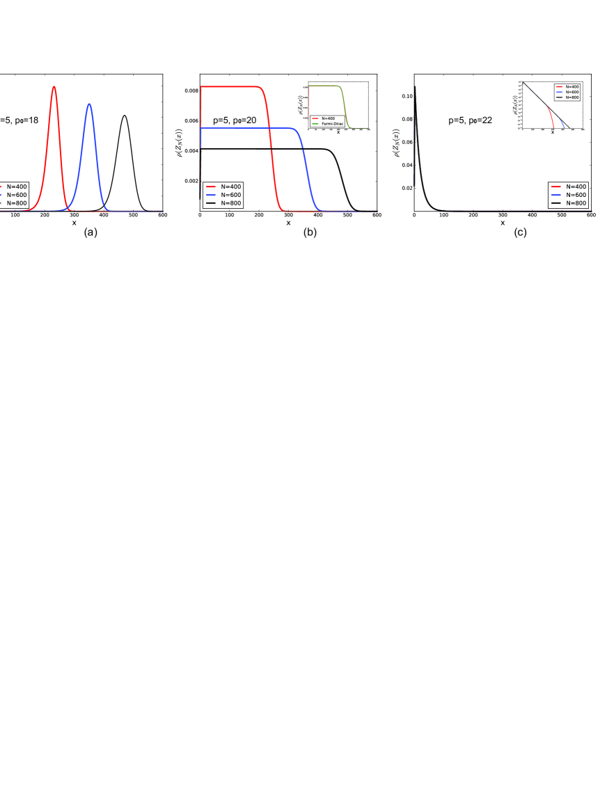
Figure 4: The distribution of the the trajectory endpoint $\rho(Z_{N}(x))=Z(N,x|p,p_{0})\left[\bar{Z}(N|p,p_{0})\right]^{-1}$ as a function of $x$ (a) the localization transition, (b) at the transition point (Insert: numerical results a fitted by the Fermi-Dirac distribution with the Fermi-energy$e_{F}=\bar{x}=\frac{p-2}{p}N$) and (c) in the localized phase (Inset: in the logarithmic scale).

IV Path counting on decorated star graphs and regular hyperbolic graphs

Here we aim to generalize the above results for two classes of more general graphs. One class, called a “decorated star graph”, is shown on Fig.5a, it consists of $p_{0}$ bundles such that each bundle has an overall linear topology, but all vertices in the bundle have functionality $p$. The second class is a class of “regular hyperbolic graphs” with special point at the origin (see Fig.5b). Here, once again, $p_{0}$ bonds are originating from the root and each vertex except the root has functionality $p$. However, among $p$ bonds originating from a node at distance $x$ from the root, one bond is going “down” to a point at distance $(x-1)$, $(p-b-1)$ are going “up” to points at distance $(x+1)$, and $b$ “horizontal” bonds connect the node with others at the same distance $x$ from the origin.

Clearly, star graphs considered in the Introduction are decorated stars with $p=2$, while regular trees with heavy root considered in sections II-III are regular hyperbolic graphs with $b=0$. In this section we aim to understand how the additional parameter, $p$ in the first case, and $b$ in the second, influences the localization transition point. Since the mathematical structure of these two problems is extremely similar, we discuss them in parallel.

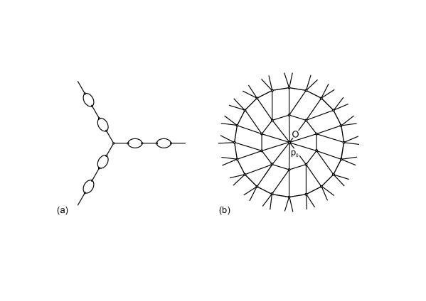
Figure 5: Decorated star graphs: (a) Simplest decorated star graph with $p_{0}=p=3$; (b) Generic decorated graph with $p_{0}=10,p=5,b=2$.

Consider first a decorated star graph. The partition function, $Z_{N}(x)$, of all $N$-step paths on such a graph, starting at the origin and ending at some distance $x$ from the root (regardless of which particular branch it is on), satisfies the recursion (compare with (19))

$$\left\{\begin{array}[]{rcll}\displaystyle Z_{N+1}(x)&=&Z_{N}(x-1)+(p-1)Z_{N}(x+1),&\quad x=2k+1\ (k\geq 1)\vskip 6.0pt plus 2.0pt minus 2.0pt\\ \displaystyle Z_{N+1}(x)&=&(p-1)Z_{N}(x-1)+Z_{N}(x+1),&\quad x=2k\ (k\geq 1)\vskip 6.0pt plus 2.0pt minus 2.0pt\\ \displaystyle Z_{N+1}(x)&=&p_{0}Z_{N}(x-1)+(p-1)Z_{N}(x+1),&\quad x=1\vskip 6.0pt plus 2.0pt minus 2.0pt\\ Z_{N+1}(x)&=&Z_{N}(x+1),&\quad x=0\vskip 6.0pt plus 2.0pt minus 2.0pt\\ Z_{N}(x)&=&0,&\quad x\leq-1\vskip 6.0pt plus 2.0pt minus 2.0pt\\ Z_{N=0}(x)&=&\delta_{x,0},\end{array}\right.$$ (44)

Results of direct iterations of (44) presented in Fig.6 show that depending on values of vertex degrees, $p$ and $p_{0}$, the localization of the trajectories may or may not exist: one clearly sees different behavior of $Z(N,x|p,p_{0})$ as a function of $x$ for few values of $p_{0}$ above and below the transition point, $\bar{p}_{0}=p$.

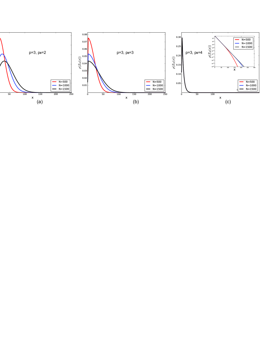
Figure 6: The distribution of the the trajectory endpoint $\rho(Z_{N}(x))=Z(N,x|p,p_{0})\left[\bar{Z}(N|p,p_{0})\right]^{-1}$ as a function of $x$ (a) below the localization transition, (b) at the transition point and (c) in the localized phase (Inset: in the logarithmic scale).

As previously discussed in Section II, half of the values of the partition function $Z_{N}(x)$ (those corresponding to odd values of $(N+x)$) equal zero. Therefore, without loss of information one can replace $Z_{N}(x)$ by $V_{N}(y)$ defined as follows:

$$\left\{\begin{array}[]{rcll}V_{N}(y)&=&\displaystyle Z_{N}(2y-1)+Z_{N}(2y),&k\geq 1\vskip 6.0pt plus 2.0pt minus 2.0pt\\ V_{N}(0)&=&Z_{N}(0)\\ \end{array}\right.$$ (45)

This new partition function $V_{N}(k)$ satisfies

$$\left\{\begin{array}[]{rcll}\displaystyle V_{N+1}(k)&=&V_{N}(k-1)+(p-2)V_{N}(k)+V_{N}(k+1),&\quad k>1\vskip 6.0pt plus 2.0pt minus 2.0pt\\ \displaystyle V_{N+1}(k)&=&p_{0}V_{N}(k-1)+(p-2)V_{N}(k)+V_{N}(k-1),&\quad k=1\vskip 6.0pt plus 2.0pt minus 2.0pt\\ V_{N+1}(k)&=&V_{N}(k+1),&\quad k=0\vskip 6.0pt plus 2.0pt minus 2.0pt\\ V_{N}(k)&=&0,&\quad k\leq-1\vskip 6.0pt plus 2.0pt minus 2.0pt\\ V_{N=0}(k)&=&\delta_{k,0},\end{array}\right.$$ (46)

It turns out that this set of equations is nothing but the set of equations describing the path counting problem on regular hyperbolic graphs defined above for a particular case of $b=p-2$.

Indeed, writing down explicitly the recursion relation for a regular hyperbolic graph one gets:

$$\left\{\begin{array}[]{rcll}\displaystyle Z_{N+1}(x)&=&(p-b-1)Z_{N}(x-1)+bZ_{N}(x)+Z_{N}(x+1),&\quad x>1\vskip 6.0pt plus 2.0pt minus 2.0pt\\ \displaystyle Z_{N+1}(x)&=&p_{0}Z_{N}(x-1)+bZ_{N}(x)+Z_{N}(x-1),&\quad x=1\vskip 6.0pt plus 2.0pt minus 2.0pt\\ Z_{N+1}(x)&=&Z_{N}(x+1),&\quad x=0\vskip 6.0pt plus 2.0pt minus 2.0pt\\ Z_{N}(x)&=&0,&\quad x\leq-1\vskip 6.0pt plus 2.0pt minus 2.0pt\\ Z_{N=0}(x)&=&\delta_{x,0},\end{array}\right.$$ (47)

In what follows we solve the more general case of Eq.(47), and then obtain the result for decorated star graphs substituting $b=p-2$ in the final expression. The solution below is completely analogous to what is presented above in Section III. Making a shift $x\to x+1$ and symmetrizing (47) by substitution:

$$Z_{N}(x)=(p-b-1)^{N/2}(p-b-1)^{x/2}W_{N}(x),$$ (48)

results in

$$\left\{\begin{array}[]{rlll}W_{N+1}(x)&=&\displaystyle W_{N}(x-1)+W_{N}(x+1)+\frac{b}{\sqrt{p-b-1}}W_{N}(x)+\\ &+&\displaystyle\frac{p_{0}-(p-b-1)}{p-b-1}\,\delta_{x,2}\,W_{N}(x-1)-\frac{b}{\sqrt{p-b-1}}\,\delta_{x,1}\,W_{N}(x),&\qquad x\geq 1\vskip 6.0pt plus 2.0pt minus 2.0pt\\ W_{N}(x)&=&0,&\qquad x=0\vskip 6.0pt plus 2.0pt minus 2.0pt\\ W_{N=0}(x)&=&\displaystyle\frac{\delta_{x,1}}{\sqrt{p-b-1}}\end{array}\right.$$ (49)

Performing the $\sin$-Fourier transform for the generating function (similarly to (24)–(25)) we obtain an integral equation

$$\frac{\tilde{{\cal W}}(s,q)}{s}-\displaystyle\frac{\sin q}{s\sqrt{p-b-1}}=(2\cos q+B)\,\tilde{{\cal W}}(s,q)+\frac{2}{\pi}\left[A\sin 2q-B\sin q\right]\int_{0}^{\pi}\tilde{{\cal W}}(s,q)\sin q\,dq$$ (50)

where

$$\tilde{{\cal W}}(s,q)=\sum_{x=0}^{\infty}{\cal W}(s,x)\sin qx,\qquad{\cal W}(s,x)=\sum_{N=0}^{\infty}W_{N}(x)s^{N}$$ (51)

and

$$A=\frac{p_{0}-(p-b-1)}{p-b-1},\qquad B=\frac{b}{\sqrt{p-b-1}}.$$ (52)

Expressing $\tilde{\cal W}$ from (50) and integrating over $q$, $q\in[0,\pi]$ with the weight $\sin q$, we obtain

$$I(s)=\displaystyle\int_{0}^{\pi}\tilde{{\cal W}}(s,q)\sin q\,dq=\frac{1}{\sqrt{p-b-1}}\int_{0}^{\pi}\frac{\sin^{2}q}{1-2s\cos q-Bs}\,dq\\ +\frac{2s}{\pi}\,I(s)\,\left[A\int_{0}^{\pi}\frac{\sin q\sin 2q}{1-2s\cos q-Bs}\,dq-B\int_{0}^{\pi}\frac{\sin^{2}q}{1-2s\cos q-Bs}\,dq\right]$$ (53)

The solution of (53) reads

$$I(s)=\frac{\pi\sqrt{p-b-1}\left(1-Bs-\sqrt{(1-Bs)^{2}-4s^{2}}\right)}{4s^{2}-\displaystyle A\left(1-Bs-\sqrt{(1-Bs)^{2}-4s^{2}}\right)^{2}+2Bs\left(1-Bs-\sqrt{(1-Bs)^{2}-4s^{2}}\right)}$$ (54)

Performing the inverse Fourier transform, one gets an explicit expression for the generating function ${\cal W}(s,x)$:

$${\cal W}(s,x)=\frac{2}{\pi}\int_{0}^{\pi}\tilde{{\cal W}}(s,q)\sin qx\,dq\\ =\frac{1}{s^{2}\sqrt{p-b-1}}\left(\frac{1-Bs-\sqrt{(1-Bs)^{2}-4s^{2}}}{2s}\right)^{x}\left[1+\frac{2}{\pi}\sqrt{p-b-1}\,I(s)(2A-Bs)\right]$$ (55)

Finally, proceeding in a way analogous to the one in Section III, we obtain an explicit expression for the generating function $Z(\sigma|p,p_{0})$ of all paths of length $N$:

$$\bar{{\cal Z}}(\sigma|p,p_{0})\equiv\sum_{x=0}^{\infty}(p-b-1)^{x/2}{\cal W}(\sigma\sqrt{p-b-1},x)=\\ =\frac{1}{\sigma(p-b-1)}\frac{1}{2\sigma-1+b\sigma+\sqrt{(1-b\sigma)^{2}-4\sigma^{2}(p-b-1)}}\times\vskip 6.0pt plus 2.0pt minus 2.0pt\\ \times\left[1+\displaystyle\frac{2}{\pi}I(\sigma\sqrt{p-b-1})\left(2\,\frac{p_{0}-(p-b-1)}{p-b-1}-b\right)\right].$$ (56)

This function, once again has three singularities: the branching point of the square root (56):

$$\sigma_{1}=\frac{1}{b+2\sqrt{p-b-1}}.$$ (57)

corresponding to the border of the continuous spectrum, the zero of the denominator of (56)

$$\sigma_{2}=\frac{1}{p}$$ (58)

corresponding to the spreading wave solution, and the third singularity, $\sigma_{3}$, corresponding to the zero of the denominator of $I(\sigma\sqrt{p-b-1})$ (see (54)), which correspond to the localized solution. Substituting $\sigma_{2}$ into equation for $\sigma_{3}$ provides the condition for critical value of $p_{0}$ which separates localized and delocalized regimes for regular hyperbolic graphs:

$$\bar{p}_{0}=p(p-b-1),$$ (59)

for decorated star graphs $b=p-2$ and this condition reduces to simple $\bar{p}_{0}=p$ in full agreement with numerical simulations presented above, while for a tree-like graph ($G$) with $b=0$, (59) is reduced to (40).

It seems interesting to compare the statistics of trajectories on the simplest star-like graph $G$, shown in the Fig.1a and on the decorated one, $G_{d}$, depicted in the Fig.5a. The mean-square displacement of the end of $N$-step path on a single branch of $G$ and of $G_{d}$, scales as $\sqrt{N}$ in both cases (with different numeric coefficients). Besides, the trajectories on the graph $G$ are localized for $p_{0}\geq 3$, and on the decorated graph $G_{d}$ the localization occurs at $p_{0}\geq 4$ (for $p_{0}=3$ the paths on $G_{d}$ are delocalized).

V Discussion

In this paper we study localization properties for a path counting problem on several classes of regular graphs with a single special vertex (trees with a ”heavy” root, decorated stars and regular hyperbolic graphs). Generalizing the argument of ternovsky we show that in all those cases the special vertex with functionality larger than that of the regular ones, works as an entropic trap for the paths on the graph, and may lead, if the trap is strong enough, to a path localization.

We used two different techniques: the study of the spectral properties of the graph adjacency matrix for finite graphs, and the study of singularities of the grand canonical partition function in case of infinite graphs. In our opinion, parallel consideration of these two approaches has in itself a significant methodical value, allowing the reader to see the similarity of these methods, and the ways how the same values can be interpreted in two different languages.

Despite, to the best of our knowledge the results presented in this paper add some new flavor to path localization on inhomogeneous graphs and networks, they certainly are an addition to the long-standing theory of localization in disordered systems, whose development goes back all the way to the works of I.M Lifhsitz lifshitz ; pastur .

There is a variety of problems in physics of disordered systems and inhomogeneous media whose solutions (e.g., solutions of corresponding hyperbolic or parabolic equations, leading eigenvectors of corresponding operators, etc.) are localized in the vicinity of some spatial regions. Similar localization problems are often studied in polymer physics, where they correspond to a polymer chain being adsorbed at some specific locations in space: like point-like defects of texture, within some particular region of space, or in the vicinity of interfaces. Most commonly, the reason for such localization is energetic: it is due to some attractive force between localized particle or polymer chain and the absorbing substrate.

The situation described in this paper belongs to a class of problems for which the origin of localization is purely entropic and is caused exclusively by geometric reasons. Among similar problems discussed in the literature is, first of all, the localization of ideal polymer chains on regular lattices with defects discussed in burda and trapping of random walks in inhomogenious media balagurov ; donsker . Similar situations are also widely discussed in spectral geometry, where the solutions of Laplace or Helmholtz equations in regions of complex shape (e.g., obtained by gluing together several simple shapes) are studied. The principal question there consists in determining the condition on the localization of wavefunctions in these complex regions grebenkov .

The phase transition on regular graphs, though in slightly different probabilistic setting, has been discussed recently in vershik2 , where authors exhaustively described the exit boundary of random walks on homogeneous trees. They showed that the model exhibits a phase transition, manifested in the loss of ergodicity of a family of Markov measures, as a function of the parameter, which controls the local transition probabilities on the tree. We plan to analyze whether the transition found in vershik2 has direct relations to the transition described in our work.

One last remark we would like to make concerning the results obtained above, is as follows. It is seen from our results that the condition for localization to occur depends significantly on the overall geometry of the graph. Indeed, on decorated star graphs it is enough to have $p_{0}>p$ to have a localization, while on tree-like graphs one needs $p_{0}>p(p-1)\sim p^{2}$ in order for trajectories to be localized. Accordingly, it remains unclear if it is possible, by changing the graph geometry, to push the transition value $\bar{p}_{0}$ below $p$, so that localization will occur even on a graph with all vertices having the same degree $p$. One possible candidate for such a localization might be a regular random graph (i.e., a random graph whose all vertices have the same degree $p$): by chance on such graphs there is a small (of order one) number of short cycles. In principle it might be conceivable that these cycles work as entropic traps in a way similar as discussed in this paper. The localization on a family of specially prepared random regular graphs with enriched fraction of short loops has been recently studied in valba1 ; valba2 .

Note added in proof. Z. Burda pointed out that in 18 the system very similar to the one described in our Section 2, has been discussed. However, the authors of 18 considered finite tree-like graphs where there is no localization transition.