Abstract

The motion of a compact body in space and time is commonly described by the world line of a point representing the instantaneous position of the body. In General Relativity such a world-line formalism is not quite straightforward because of the strict impossibility to accommodate point masses and rigid bodies. In many situations of practical interest it can still be made to work using an effective hamiltonian or energy-momentum tensor for a finite number of collective degrees of freedom of the compact object. Even so exact solutions of the equations of motion are often not available. In such cases families of world lines of compact bodies in curved space-times can be constructed by a perturbative procedure based on generalized geodesic deviation equations. Examples for simple test masses and for spinning test bodies are presented.

1 Test bodies in General Relativity

The newtonian theory of gravity is a theory of instantaneous action at a distance, which is consistent with the concept of absolute time and absolute simultaneity. This allows for the existence of rigid bodies. Taking that for granted Newton proved in the Principia that the orbital motion of a homogeneous spherical rigid body is correctly represented by that of a point mass located at the center of gravity. Thus he was able to explain the motion of the moon orbiting the earth. Also in more general situations the motion of a rigid body can be represented by a single curve: its world line, identified as the orbit in space and time of the center of gravity, whilst the remaining kinematical degrees of freedom are restricted to rotational motion of the body about the center of gravity and specify the orientation of the body at every point of the world line. In this frame work there is no obstacle to consider the limit of a very small rigid body of which the gravitational influence on the motions of other bodies is negligeable. Such a body which probes the gravitational field without disturbing it is commonly referred to as a test body. It is characterized by a finite number of physical degrees of freedom as its motion is completely specified in terms of its world line plus orientational degrees of freedom.

In General Relativity (GR) the situation is more subtle, as strictly point-like particles cannot be accommodated in the theory. Most importantly any object of finite non-zero mass $m$ has an associated Schwarzschild radius

$$\rho_{S}=\frac{2Gm}{c^{2}},$$

such that if the size of the object shrinks below this scale it becomes a black hole with a finite surface area equal to $A=4\pi\rho_{S}^{2}$ for spherical bodies. Thus any massive body is an extended body, at least in classical GR. In situations where quantum effects become relevant this may change, but then there are other limitations like the Compton wave length opposing complete localization of objects.

If a classical object also possesses an internal angular momentum (spin) there are additional complications. First of all in GR rigid bodies can not exist and there is no unique, observer-independent center of mass. Indeed as there is no absolute simultaneity the relative positions of different particles composing the body at any fixed time depend on the state of motion of the body with respect to the observer. Some elementary considerations showing this state of affairs are discussed for a simple two-body system in appendix A. In addition, in a relativistic context for a composite system it is more appropriate to discuss the motion of a center of energy or centroid rather than a center of mass, although such a concept is still observer-dependent. Actually it has been shown [1, 2, 3] that under reasonable assumptions the world lines of all possible centroids of an object with mass $m$ and spin $s$ fill a time-like oriented tube of radius

$$\rho_{M}=\frac{s}{mc}.$$

The upshot of this discussion is that strictly speaking in GR no unique world line can be associated with the motion of massive bodies and any particular choice of representative world line is at least in part a matter of convenience and requires careful specification.

Nevertheless there are circumstances in which the localization of a compact body is possible with sufficient accuracy that for practical purposes it may be regarded as a mass point moving along a world line. Moreover if its mass is small enough that one can neglect the associated space-time curvature and its influence on other bodies, one can still regard such an approximate point mass as a test body probing the space-time geometry in which it moves.

In the context of GR the space-time geometry and the motion of compact bodies are linked by the Einstein equations

$$G_{\mu\nu}+8\pi G\,T_{\mu\nu}=0,$$ (1)

where the Einstein tensor $G_{\mu\nu}$ is specified by the space-time geometry, and the energy-momentum tensor $T_{\mu\nu}$ describes the physical degrees of matter. Irrespective of the precise background geometry the Bianchi identities for the Einstein tensor require the energy-momentum tensor to be divergence-free:

$$\nabla_{\mu}T^{\mu\nu}=0.$$ (2)

For a compact body with mass $m$ moving as an approximate point mass along a world line $\xi^{\mu}(\tau)$ parametrized by the proper time $\tau$ the effective energy-momentum tensor is [4]

$$T^{\mu\nu}(x)=\frac{m}{\sqrt{-g}}\,\int d\tau\,\dot{\xi}^{\mu}\dot{\xi}^{\nu}\delta^{4}(x-\xi(\tau)),$$ (3)

with the overdot denoting a derivative w.r.t. proper time. Its divergence vanishes if the world line is a geodesic:

$$\nabla_{\mu}T^{\mu\nu}=\frac{m}{\sqrt{-g}}\,\int d\tau\left[\ddot{\xi}^{\nu}+\Gamma_{\mu\lambda}^{\;\;\;\nu}(\xi)\dot{\xi}^{\mu}\dot{\xi}^{\lambda}\right]\delta^{4}(x-\xi(\tau))=0.$$ (4)

Neglecting the back reaction of the compact body is allowed if the contributions of the test body to the geometry of space time are too small to be of interest. As an illustration take the local background geometry to be that of flat Minkowski space-time:

$$g^{(0)}_{\mu\nu}=\eta_{\mu\nu}\hskip 10.00002pt\mbox{and}\hskip 10.00002pt\Gamma^{(0)\;\nu}_{\mu\lambda}=0.$$ (5)

In particular we can then choose to work in the local inertial frame in which the body is at rest:

$$T^{(0)}_{00}=m\delta^{3}(\mathbb{x}),\hskip 10.00002ptT^{(0)}_{i0}=T^{(0)}_{ij}=0\hskip 20.00003pti,j=(1,2,3).$$ (6)

Taking into account these energy-momentum source terms, the solution of the Einstein equation is modified to first order to read

$$g^{(1)}_{\mu\nu}=\eta_{\mu\nu}+h_{\mu\nu},$$ (7)

where the correction term satisfies the linearized Einstein equation

$$\begin{array}[]{l}\Box h_{\mu\nu}-\partial_{\mu}\partial^{\lambda}h_{\lambda\nu}-\partial_{\nu}\partial^{\lambda}h_{\lambda\mu}+\partial_{\mu}\partial_{\nu}h_{\lambda}^{\;\,\lambda}-\eta_{\mu\nu}\left(\Box h_{\lambda}^{\;\,\lambda}-\partial^{\kappa}\partial^{\lambda}h_{\kappa\lambda}\right)\\ \\ =-8\pi G\,T^{(0)}_{\mu\nu}.\end{array}$$ (8)

Removing gauge degress of freedom by the De Donder conditions

$$\partial^{\mu}h_{\mu\nu}=\frac{1}{2}\,\partial_{\nu}h_{\mu}^{\;\,\mu},$$

the Einstein equation simplifies further to

$$\Box\left(h_{\mu\nu}-\frac{1}{2}\,\eta_{\mu\nu}h_{\lambda}^{\;\lambda}\right)=-16\pi G\,T^{(0)}_{\mu\nu},$$ (9)

which has the solution

$$h_{i0}=0,\hskip 10.00002pth_{ij}=\delta_{ij}h_{00},\hskip 10.00002pth_{00}=\frac{2Gm}{r}.$$ (10)

With this correction we obtain the modified line element

$$g^{(1)}_{\mu\nu}dx^{\mu}dx^{\nu}=-\left(1-\frac{2Gm}{r}\right)dt^{2}+\left(1+\frac{2Gm}{r}\right)d\mathbb{r}^{2}.$$ (11)

It follows that the geometry near the test body deviates strongly from flat space on the scale of its Schwarzschild radius, and it can be considered as a near point-like object only as long as the external curvature is comparatively small on this scale.

Actually to first order in $G$ the geometry specified by the line element (11) coincides with that of Schwarzschild space-time in isotropic co-ordinates:

$$g_{\mu\nu}dx^{\mu}dx^{\nu}=-\left(\frac{2r-Gm}{2r+Gm}\right)^{2}dt^{2}+\left(1+\frac{Gm}{2r}\right)^{4}d\mathbb{r}^{2}.$$ (12)

In hindsight it is not such a surprise that the test-particle approximation is the limit of a black-hole geometry, as it is well-known that the standard black-hole space-times are exact vacuum solutions of the Einstein equations characterized by a finite number of parameters like mass, spin and electric charge, in which respect they resemble test bodies. The difference is of course that their action on the space-time geometry has been fully taken into account to the extent that –in contrast to test particles– their energy-momentum tensor has been absorbed completely in the space-time curvature, i.e. it has become part of the Einstein tensor in eqn. (1).

2 The motion of test bodies

Restricting our considerations to situations where the internal degrees of freedom of a compact body do not take part in its gravitational interaction and its size and gravitational back reaction can be neglected, its motion can be represented adequately by a world line which is a time-like geodesic of the external space-time geometry. This is the simplest case of the test-body approximation. The more elaborate test-body limit of a compact body with spin will be discussed in sects. 4 and later.

This description of a test body as an object with a finite numer of degrees of freedom to which one can assign at any moment a representative position has considerable mathematical advantage: to such a body we can associate a finite-dimensional phase space in which the evolution of the system is described by a simple curve. This orbit is generated by a hamiltonian $H$ depending on a finite number of phase-space variables including position and momentum. As by construction it neglects the finite size and gravitational back reaction of the body, it is of course an effective hamiltonian, its validity restricted by the test-body limit.

The effective hamiltonian dynamics of a massive test body with no other degrees of freedom, like spin or charge, and an energy-momentum tensor of the form (1) is straightforward to construct. The phase space is spanned by the position variables $\xi^{\mu}(\tau)$ and the momentum variables $\pi_{\mu}(\tau)$, with the usual equal proper-time canonical Poisson brackets

$$\left\{\xi^{\mu},\pi_{\nu}\right\}=\delta_{\nu}^{\mu}.$$ (13)

The free hamiltonian

$$H=\frac{1}{2m}\,g^{\mu\nu}[\xi]\,\pi_{\mu}\pi_{\nu}$$ (14)

then generates the equations of motion

$$\dot{\xi}^{\mu}=\left\{\xi^{\mu},H\right\}=\frac{1}{m}\,g^{\mu\nu}\pi_{\nu},\hskip 20.00003pt\dot{\pi}_{\mu}=\left\{\pi_{\mu},H\right\}=\frac{1}{2m}\,\partial_{\mu}g^{\nu\lambda}\,\pi_{\nu}\pi_{\lambda}.$$ (15)

By simple algebra these equations can be rewritten in the form

$$\pi_{\mu}=mg_{\mu\nu}\dot{\xi}^{\nu},\hskip 20.00003pt\ddot{\xi}^{\mu}+\Gamma_{\lambda\nu}^{\;\;\;\mu}\dot{\xi}^{\lambda}\dot{\xi}^{\nu}=0,$$ (16)

reproducing the geodesic equation derived earlier from the energy-momentum tensor (1).

In this hamiltonian frame work it is easy to find constants of motion, simplifying the solution of the geodesic equation. There is at least one universal constant independent of the specific metric $g_{\mu\nu}$, the hamiltonian itself:

$$H=-\frac{m}{2}\hskip 10.00002pt\Leftrightarrow\hskip 10.00002ptg_{\mu\nu}\,\dot{\xi}^{\mu}\dot{\xi}^{\nu}=-1.$$ (17)

It establishes the usual relation between proper time and co-ordinate time. Other constants of motion depend on the symmetries of the background space-time, as implied by Noether’s theorem. For example a quantity

$$J[\xi,\pi]=\alpha^{\mu}[\xi]\,\pi_{\mu}$$ (18)

is a constant of motion if $\alpha^{\mu}$ is a Killing vector, representing an isometry of the metric:

$$\dot{J}=\left\{J,H\right\}=0\hskip 10.00002pt\Leftrightarrow\hskip 10.00002pt\nabla_{\mu}\alpha_{\nu}+\nabla_{\nu}\alpha_{\mu}=0.$$ (19)

As an example in static space-times the kinetic energy $E$ of the test body is a constant of motion:

$$\alpha^{\mu}=(-1,0,0,0)\hskip 10.00002pt\Rightarrow\hskip 10.00002ptE=-\pi_{t}.$$ (20)

In particular in Minksowki space-time:

$$E=-m\,\eta_{tt}\,\dot{\xi}^{t}=m\,\frac{dt}{d\tau}=\gamma m,$$ (21)

where $\gamma$ is the time-dilation factor.

In spherically symmetric geometries, such as Minkowski, Schwarzschild and Freedmann-Lemaitre type cosmological space-times, all three components of angular momentum are conserved:

$$\begin{array}[]{l}J_{1}=-\sin\varphi\,\pi_{\theta}-\mbox{\,cotan\,}\theta\,\cos\varphi\,\pi_{\varphi},\\ \\ J_{2}=\cos\varphi\,\pi_{\theta}-\mbox{\,cotan\,}\theta\,\sin\varphi\,\pi_{\varphi},\\ \\ J_{3}=\pi_{\varphi}.\end{array}$$ (22)

Here the momenta $(\pi_{r},\pi_{\theta},\pi_{\varphi})$ are defined w.r.t. a polar co-ordinate frame $(r,\theta,\varphi)$ such that the hamiltonian is given by

$$2mH=-g^{tt}(t,r)\pi_{t}^{2}+g^{rr}(t,r)\pi_{r}^{2}+g^{\theta\theta}(t,r)\left(\pi_{\theta}^{2}+\frac{\pi_{\varphi}^{2}}{\sin^{2}\theta}\right).$$ (23)

Clearly if the metric components $g_{\mu\nu}$ are time independent the system is both static and spherically symmetric, and energy an angular momentum are all conserved. This holds in particular for Minkowski and Schwarzschild space-time.

The standard metric of Schwarzschild space-time in Droste co-ordinates for an object with mass $M$ can be obtained from the isotropic co-ordinate representation (12) by the co-ordinate transformation

$$\bar{r}=r\left(1+\frac{GM}{2r}\right)^{2},$$ (24)

reproducing the static, spherically symmetric line element

$$g_{\mu\nu}dx^{\mu}dx^{\nu}=-\left(1-\frac{2GM}{\bar{r}}\right)dt^{2}+\frac{d\bar{r}^{2}}{1-\frac{2GM}{\bar{r}}}+\bar{r}^{2}\left(d\theta^{2}+\sin^{2}\theta\,d\varphi^{2}\right).$$ (25)

Replacing $\bar{r}\rightarrow r$ we can then write the hamiltonian for a test body in Schwarzschild space-time as

$$2mH=-\frac{\pi_{t}^{2}}{1-\frac{2GM}{r}}+\left(1-\frac{2GM}{r}\right)\pi_{r}^{2}+\frac{1}{r^{2}}\left(\pi_{\theta}^{2}+\frac{\pi_{\varphi}^{2}}{\sin^{2}\theta}\right),$$ (26)

which is a special instance of a static hamiltonian of the type (23). The conservation of kinetic energy then holds in the form

$$\varepsilon\equiv\frac{E}{m}=\left(1-\frac{2GM}{r}\right)\frac{dt}{d\tau}.$$ (27)

Rotating the co-ordinate system such that the plane of the orbit is at constant $\theta=\pi/2$, we have $J_{1}=J_{2}=\pi_{\theta}=0$ and

$$\ell\equiv\frac{J_{3}}{m}=r^{2}\,\frac{d\varphi}{d\tau}.$$ (28)

In addition the universal constant of motion $H=-m/2$ implies that

$$\left(\frac{dr}{d\tau}\right)^{2}=\varepsilon^{2}-\left(1-\frac{2GM}{r}\right)\left(1+\frac{\ell^{2}}{r^{2}}\right).$$ (29)

In particular there are circular orbits $r=R=$ constant for which

$$\begin{array}[]{l}\displaystyle{\frac{d\varphi}{d\tau}=\frac{\ell}{R^{2}}=\sqrt{\frac{GM}{R^{3}}}\,\frac{1}{\sqrt{1-\frac{3GM}{R}}},}\\ \\ \displaystyle{\frac{dt}{d\tau}=\frac{\varepsilon}{1-\frac{2GM}{R}}=\frac{1}{\sqrt{1-\frac{3GM}{R}}}.}\end{array}$$ (30)

Observe that these equations reproduce Keplers third law for circular orbits:

$$\frac{d\varphi}{dt}=\sqrt{\frac{GM}{R^{3}}}\hskip 10.00002pt\Rightarrow\hskip 10.00002ptT^{2}=\frac{4\pi^{2}}{GM}\,R^{3},$$

where $T$ is the orbital period measured by the clock of a distant observer keeping co-ordinate time $t$, and the radial co-ordinate $R$ is determined by the orbital circumference through the relation $L=2\pi R$.

3 Geodesic deviations

In most space-time geometries general exact solutions of the geodesic equation are difficult to obtain, and when they are available they are often expressed in terms of non-elementary transcendental functions [5]. However given one particular geodesic curve it is possible to find approximate solutions for arbitrary nearby geodesics using the geodesic deviation equation and its higher-order generalizations [6, 7]. This procedure can also be explained in terms of the Schild ladder construction [8, 9], for which next-to-leading order corrections can be obtained using the results reviewed in this section.

In terms of the tangent vector $u^{\mu}=\dot{\xi}^{\mu}$ the geodesic equation (16) reads

$$D_{\tau}u^{\mu}=\dot{u}^{\mu}+\Gamma_{\lambda\nu}^{\;\;\;\mu}u^{\lambda}u^{\nu}=0.$$ (31)

Now consider a family of world lines

$$\xi^{\mu}(\tau,\sigma)=\xi^{\mu}(\tau)+\sigma n^{\mu}(\tau),$$ (32)

obtained by a displacement of the geodesic in the direction of a vector field $n^{\mu}(\tau)$ scaled by the real parameter $\sigma$. The corresponding changes in the world line and its tangent vector are described covariantly by the vectors

$$\Delta\xi^{\mu}=\sigma n^{\mu},\hskip 10.00002pt\Delta u^{\mu}=D_{\tau}\Delta\xi^{\nu}=\sigma D_{\tau}n^{\mu}.$$ (33)

For this displacement to respect the geodesic equation (31) to first order in $\sigma$ we require

$$\Delta D_{\tau}u^{\mu}=D_{\tau}\Delta u^{\mu}+\left[\Delta,D_{\tau}\right]u^{\mu}=\sigma\left(D_{\tau}^{2}\,n^{\mu}-R_{\lambda\nu\kappa}^{\;\;\;\;\;\,\mu}u^{\lambda}u^{\kappa}n^{\nu}\right)=0.$$ (34)

For example, we know all circular orbits in Schwarzschild space-time in analytical form. Then we can construct approximate non-circular (eccentric) solutions in the same plane by adding a geodesic deviation $\sigma n^{\mu}$; generically this is an oscillating term as the test body moves periodically closer and farther from the central mass between periastron and apastron. As the period of this perturbation is in general different from the period of the circular orbit one starts from, the periastron and apastron will shift their azimuthal directions each turn. This phenomenon is well-known ever since it was calculated by Einstein for the planet Mercury in its orbit around the sun. It turns out that for Mercury the first-order deviation (33) from motion on a circle with the period of Mercury’s orbit actually already gives full numerical agreement with the observed periastron shift of 43 arcseconds per century [6].

There is however no obstacle to include second and higher-order contributions in $\sigma$ to the displaced geodesics $\xi^{\mu}(\sigma,\tau)$. As $\Delta$ creates a covariant displacement in the direction of $n$, but $n$ is not necessarily displaced parallel to itself (it is not required to be a tangent vector field to a family of geodesics crossing the world line $\xi^{\mu}(\tau)$), it follows that in general

$$\Delta^{2}\xi^{\mu}=\sigma\Delta n^{\mu}\equiv\sigma^{2}m^{\mu}\neq 0.$$ (35)

The geodesic family $\xi^{\mu}(\tau,\sigma)$ is then parametrized to second order in $\sigma$ by

$$\xi^{\mu}(\tau,\sigma)=\xi_{1}^{\mu}(\tau)+\sigma n^{\mu}(\tau)+\frac{1}{2}\,\sigma^{2}\left(m^{\mu}-\Gamma_{\lambda\nu}^{\;\;\;\mu}n^{\lambda}n^{\nu}\right)+....$$ (36)

Using the properties of the vector field $n$ it is straightforward to generalize the derivation of eq. (34) and show that $(n^{\mu},m^{\mu},...)$ are solutions of a hierarchy of deviation equations [6]

$$\begin{array}[]{lll}\displaystyle{D_{\tau}^{2}n^{\mu}-R_{\lambda\nu\kappa}^{\;\;\;\;\;\,\mu}u^{\kappa}u^{\lambda}n^{\nu}}&=&0,\\ &&\\ \displaystyle{D_{\tau}^{2}m^{\mu}-R_{\lambda\nu\kappa}^{\;\;\;\;\;\,\mu}u^{\kappa}u^{\lambda}m^{\nu}}&=&\displaystyle{\left(\nabla_{\rho}R_{\kappa\nu\lambda}^{\;\;\;\;\;\,\mu}-\nabla_{\kappa}R_{\rho\lambda\nu}^{\;\;\;\;\;\,\mu}\right)u^{\kappa}u^{\lambda}n^{\rho}n^{\nu}}\\ \\ &&\displaystyle{+4R_{\kappa\nu\lambda}^{\;\;\;\;\;\,\mu}u^{\kappa}n^{\nu}D_{\tau}n^{\lambda},}\\ \\ ...\end{array}$$ (37)

We note in passing, that whereas the first-order deviations $n^{\mu}$ provide information about the curvature of space-time through the Riemann tensor $R_{\kappa\nu\lambda\mu}$, the second-order deviations provide further information about the gradient $\nabla_{\rho}R_{\kappa\nu\lambda\mu}$ of the Riemann tensor. Thus with sufficient knowledge of families of geodesics in some domain of space-time one can reconstruct the Riemann tensor in the whole domain in terms of a Taylor series from the geodesic deviations w.r.t. a given geodesic [10, 11, 12].

The procedure described here has been worked out for Schwarzschild space-time up to and including the second-order deviations [6, 13, 14]. The results for orbits in the equatorial plane $\theta=\pi/2$ are summarized by the parametrized expansions

$$\begin{array}[]{lll}\displaystyle{t(\tau,\sigma)=\xi_{0}^{t}(\sigma)\tau+\sum_{n=1}^{\infty}\,\xi_{n}^{t}(\sigma)\sin n\omega(\sigma)\tau,}\\ \\ \displaystyle{r(\tau,\sigma)=\xi_{0}^{r}(\sigma)+\sum_{n=1}^{\infty}\,\xi_{n}^{r}(\sigma)\cos n\omega(\sigma)\tau,}\\ \\ \displaystyle{\varphi(\tau,\sigma)=\xi_{0}^{\varphi}(\sigma)\tau+\sum_{n=1}^{\infty}\,\xi_{n}^{\varphi}(\sigma)\sin n\omega(\sigma)\tau.}\\ \end{array}$$ (38)

The coefficients $\xi_{n}^{\mu}(\sigma)$ and the fundamental frequency $\omega(\sigma)$ are computed order by order in $\sigma$ by solving the hierarchy of deviation equations (37). Of course the terms of order $\sigma^{0}$ represent the parameters of the circular parent orbit we encountered in eqs. (30):

$$\xi_{0}^{t}(0)=\frac{1}{\sqrt{1-\frac{3GM}{R}}},\hskip 10.00002pt\xi_{0}^{r}(0)=R,\hskip 10.00002pt\xi_{0}^{\varphi}(0)=\sqrt{\frac{GM}{R^{3}}}\,\frac{1}{\sqrt{1-\frac{3GM}{R}}}.$$ (39)

All other terms have non-trivial dependence on the expansion parameter $\sigma$:

$$\begin{array}[]{l}\displaystyle{\xi_{0}^{\mu}(\sigma)=\xi_{0}^{\mu}(0)+\sigma\rho_{1}^{\mu}+\frac{1}{2}\,\sigma^{2}\rho_{2}^{\mu}+...,}\\ \\ \displaystyle{\xi_{1}^{\mu}(\sigma)=\sigma n_{1}^{\mu}+\frac{1}{2}\,\sigma^{2}n_{2}^{\mu}+...,}\\ \\ \displaystyle{\xi_{2}^{\mu}(\sigma)=\frac{1}{2}\,\sigma^{2}m_{2}^{\mu}+...,}\end{array}$$ (40)

each $\xi_{n}^{\mu}(\sigma)$ contributing only terms of order $\sigma^{n}$ and higher, whilst the angular frequency

$$\omega(\sigma)=\omega_{0}+\sigma\omega_{1}+...$$ (41)

also depends on the order of approximation, reflecting the anharmonicity of the non-circular deviations. The explicit expressions for the coefficients $\rho_{n}^{\mu}$, $n_{n}^{\mu}$ and $m_{n}^{\mu}$ for $n=1$ and $n=2$ and the expressions for the frequencies $\omega_{0}$, $\omega_{1}$ are summarized in appendix B for the restricted case $\rho_{n}^{r}=0$. This restriction implies, that we compare the non-circular orbits to a fixed circular orbit, although in general one might wish to adapt the circular reference orbit order by order in $\sigma$ to improve convergence. The expressions for the unrestricted case can be found in ref. [13].

Observe that the deviations are bound and periodic as long as the angular frequency $\omega$ is real. For $R<6GM$ equation (77) in the appendix shows that it develops an imaginary part, indicating exponential run-away behaviour. Thus the circular orbit with $R=6GM$ is the innermost stable circular orbit (ISCO) for a simple test body in Schwarzschild space-time.

Finally from the solutions of the geodesic deviations we can evaluate the constants of motion $\varepsilon$ and $\ell$ for the non-circular orbits by substitution of the solutions for $dt/d\tau$ and $d\varphi/d\tau$ including first and second order deviations into the expressions (27) and (28). The resulting constants of motion are then also written as a series expansion in the deviation parameter $\sigma$. Up to and including second order deviations the result is

$$\varepsilon(\sigma)=\varepsilon_{0}+\sigma\varepsilon_{1}+\frac{1}{2}\,\sigma^{2}\varepsilon_{2}+...,\hskip 10.00002pt\ell(\sigma)=\ell_{0}+\sigma\ell_{1}+\frac{1}{2}\,\sigma^{2}\ell_{2}+...,$$ (42)

where $\varepsilon_{0}$ and $\ell_{0}$ are the energy and angular momentum per unit of mass for circular orbits:

$$\varepsilon_{0}=\frac{R-2GM}{\sqrt{R(R-3GM)}},\hskip 10.00002pt\ell_{0}=\sqrt{\frac{GMR^{2}}{R-3GM}}.$$ (43)

In the restricted case $\rho^{r}_{1}=0$ the first-order corrections vanish: $\varepsilon_{1}=\ell_{1}=0$, but the second-order corrections do not:

$$\begin{array}[]{l}\displaystyle{\varepsilon_{2}=-\frac{GM}{2R^{7/2}}\,\frac{R^{2}-9GMR+6(GM)^{2}}{(R-3GM)^{3/2}},}\\ \\ \displaystyle{\ell_{2}=-\frac{3\sqrt{GM}}{2R^{2}}\,\frac{(R-2GM)(R-7GM)}{(R-3GM)^{3/2}}.}\end{array}$$ (44)

The most important aspect of these expressions is that all dependence on the proper time has disappeared and therefore they are true constants of motion indeed. This is a strong consistency check on the results listed in appendix B.

One of the useful aspects of the perturbative construction of orbits by the method of geodesic deviations is that they provide explicit and accurate expressions for the position of the test body as a function of the evolution parameter (proper time). Most results in the literature describe the time-dependence of the orbits only in an implicit way. The explicit time-dependent representation of the orbits of a test body in Schwarzschild space-time is especially useful in the computation of the emission of gravitational waves by extreme mass ratio (EMR) binaries: systems consisting of a compact stellar object, like a white dwarf, neutron star or stellar-mass black hole orbiting a supermassive black hole such as found in the center of many galaxies. Gravitational wave emission by EMR binaries has been studied in detail in ref. [14].

4 Spinning test bodies

The motion of electrically neutral, non-spinning test bodies is represented by geodesics in space-time. As soon as new degrees of freedom come into play the world line of a test body becomes non-geodesic. For example, an electrically charged particle in the presence of electric or magnetic fields is subject to a Lorentz force in addition to the effect of curvature. Its world line will differ from that of a similar neutral particle which follows a geodesic.

Similarly the effect of rotation represented by internal angular momentum (spin) will change the motion of test body in curved space-time even in the absence of other fields of force [15]-[16]. One can think of this as a form of gravitational spin-orbit coupling. In this section we discuss the motion of spinning test bodies in more detail.

There is an extended literature on spinning test particles; for a review see e.g. ref. [17]. The most common approaches are based on a multipole expansion requiring a dynamical constraint as an implicit choice of the center of mass fixing the monopole term. As this choice is not unique we have developed in refs. [18, 19, 20] a different formalism which does not incorporate any constraints but only requires appropriate initial conditions to solve the equations of motion. In this formulation the spin degrees of freedom are described by a real anti-symmetric tensor field $\Sigma^{\mu\nu}(\tau)$, which has six components defined on the world line. Three of these components can be represented equivalently by a space-like axial vector, a magnetic-type dipole moment which we identify with the spin proper. Similarly the other three components are described equivalently by a space-like real vector, an electric-type dipole moment which in the gravitational context is interpreted as a mass dipole. Denoting the four-velocity of the test body by the time-like unit vector $u^{\mu}=\dot{\xi}^{\mu}$, we can decompose the spin tensor $\Sigma^{\mu\nu}$ accordingly as follows

$$\Sigma^{\mu\nu}=-\frac{1}{\sqrt{-g}}\,\varepsilon^{\mu\nu\kappa\lambda}u_{\kappa}S_{\lambda}+u^{\mu}Z^{\nu}-u^{\nu}Z^{\mu},$$ (45)

with $S_{\mu}$ and $Z^{\mu}$ representing the proper spin and mass dipole components, respectively. The decomposition (45) can be inverted to get

$$S_{\mu}=\frac{1}{2}\,\sqrt{-g}\,\varepsilon_{\mu\nu\kappa\lambda}u^{\nu}\Sigma^{\kappa\lambda},\hskip 10.00002ptZ^{\mu}=\Sigma^{\mu\nu}u_{\nu}.$$ (46)

As mentioned both vectors are space-like by construction:

$$S\cdot u=0,\hskip 10.00002ptZ\cdot u=0.$$ (47)

Hence each contains only three degrees of freedom, their time components vanishing in the rest frame $u=(1,0,0,0)$. From these expressions it is infered directly that under the group of three-dimensional spatial rotations and parity transformations in the rest frame $Z$ is a real vector, whereas $S$ actually is an axial pseudo-vector.

To obtain equations of motion for a spinning body we follow the same route as for a non-rotating body starting from an energy-momentum tensor and rederiving the results from an effective hamiltonian. Following [19] the energy-momentum tensor is taken to have support on a world line $\xi^{\mu}(\tau)$ with

$$\begin{array}[]{lll}T^{\mu\nu}&=&\displaystyle{m\int d\tau\,u^{\mu}u^{\nu}\,\frac{1}{\sqrt{-g}}\,\delta^{4}(x-\xi(\tau))}\\ &&\\ &&\displaystyle{+\frac{1}{2}\,\nabla_{\lambda}\int d\tau\left(u^{\mu}\Sigma^{\nu\lambda}+u^{\nu}\Sigma^{\mu\lambda}\right)\frac{1}{\sqrt{-g}}\,\delta^{4}(x-\xi(\tau)).}\end{array}$$ (48)

Its covariant divergence vanishes: $\nabla_{\mu}T^{\mu\nu}=0$, if

$$\begin{array}[]{l}\displaystyle{mD_{\tau}u^{\mu}=\dot{u}^{\mu}+\Gamma_{\lambda\nu}^{\;\;\;\mu}u^{\lambda}u^{\nu}=\frac{1}{2}\,\Sigma^{\kappa\lambda}R_{\kappa\lambda\;\,\nu}^{\;\;\;\,\mu}u^{\nu},}\\ \\ \displaystyle{D_{\tau}\Sigma^{\mu\nu}=\dot{\Sigma}^{\mu\nu}+u^{\lambda}\Gamma_{\lambda\kappa}^{\;\;\;\mu}\Sigma^{\kappa\nu}+u^{\lambda}\Gamma_{\lambda\kappa}^{\;\;\;\nu}\Sigma^{\mu\kappa}=0.}\end{array}$$ (49)

Alternatively in the hamiltonian formulation we introduce a set of classical Poisson-Dirac brackets on the particle phase space defined by [18, 20]

$$\begin{array}[]{l}\displaystyle{\left\{\xi^{\mu},\pi_{\nu}\right\}=\delta^{\mu}_{\nu},\hskip 20.00003pt\left\{\pi_{\mu},\pi_{\nu}\right\}=\frac{1}{2}\,\Sigma^{\kappa\lambda}R_{\kappa\lambda\mu\nu},}\\ \\ \displaystyle{\left\{\Sigma^{\mu\nu},\pi_{\lambda}\right\}=\Gamma_{\lambda\kappa}^{\;\;\;\mu}\Sigma^{\nu\kappa}-\Gamma_{\lambda\kappa}^{\;\;\;\nu}\Sigma^{\mu\kappa},}\\ \\ \displaystyle{\left\{\Sigma^{\mu\nu},\Sigma^{\kappa\lambda}\right\}=g^{\mu\kappa}\Sigma^{\nu\lambda}-g^{\mu\lambda}\Sigma^{\nu\kappa}-g^{\nu\kappa}\Sigma^{\mu\lambda}+g^{\nu\lambda}\Sigma^{\mu\kappa}.}\end{array}$$ (50)

These brackets have several important features. First, they define an algebra with structure functions rather than structure constants. Moreover these structure functions encode all of the usual space-time geometry: the metric, the connection and the Riemann curvature tensor. In addition the properties of these geometric objects guarantee that the Jacobi identities for cyclic triple brackets are satisfied by this Poisson-Dirac algebra without specifying the dynamics of the system. Therefore the bracket algebra is consistent independently of the choice of hamiltonian. In particular the free hamiltonian (14):

$$H=\frac{1}{2m}\,g^{\mu\nu}[\xi]\,\pi_{\mu}\pi_{\nu},$$

generates the same equations of motion (49) as derived from the energy-momentum tensor, providing in addition the identification of $\pi_{\mu}$ with the kinetic momentum (16):

$$\pi_{\mu}=mg_{\mu\nu}u^{\nu}.$$

To solve the equations of motion (49) it is again convenient to first identify constants of motion. In this case there are 3 universal constants of motion, independent of the specific geometry: the hamiltonian itself:

$$H=-\frac{m}{2},$$

as long as it is proper-time independent; and two spin invariants:

$$\begin{array}[]{l}\displaystyle{I=\frac{1}{2}\,g_{\mu\kappa}g_{\nu\lambda}\Sigma^{\mu\nu}\Sigma^{\kappa\lambda}=S^{2}-Z^{2},}\\ \\ \displaystyle{D=\frac{1}{8}\,\sqrt{-g}\,\varepsilon_{\mu\nu\kappa\lambda}\Sigma^{\mu\nu}\Sigma^{\kappa\lambda}=S\cdot Z.}\end{array}$$ (51)

Clearly $I$ is a real scalar whilst $D$ is a pseudoscalar under three-dimensional spatial rotations and parity transformations.

In addition there may exist other constants of motion connected with symmetries of the background space time. The construction in equations (18), (19) based on the presence of Killing vectors can be generalized immediately to include spin [21, 22], as follows: a quantity

$$J[\xi,\pi,\Sigma]=\alpha^{\mu}[\xi]\,\pi_{\mu}+\frac{1}{2}\,\beta_{\mu\nu}[\xi]\,\Sigma^{\mu\nu}$$ (52)

is a constant of motion if $\alpha^{\mu}$ is a Killing vector and $\beta_{\mu\nu}$ its gradient:

$$\nabla_{\mu}\alpha_{\nu}+\nabla_{\nu}\alpha_{\mu}=0,\hskip 20.00003pt\beta_{\mu\nu}=-\beta_{\nu\mu}=\nabla_{\mu}\alpha_{\nu}.$$ (53)

Observe that the symmetric part of $\beta_{\mu\nu}$ vanishes by construction as a result of the Killing condition; this property also implies the identity

$$\nabla_{\lambda}\beta_{\mu\nu}=R_{\mu\nu\lambda}^{\;\;\;\;\;\,\kappa}\,\alpha_{\kappa},$$ (54)

which is necessary to show that $J$ is a constant of motion.

5 Spinning test bodies in Schwarzschild space-time

Applying the general formalism above to the case of Schwarzschild space-time we first construct the generalization of the constants of motion (20) and (22), to wit the kinetic energy based on the Killing vector of time-translation invariance:

$$E=-\pi_{t}-\frac{GM}{r^{2}}\,\Sigma^{tr}=m\left(1-\frac{2GM}{r}\right)u^{t}-\frac{GM}{r^{2}}\,\Sigma^{tr},$$ (55)

and the total angular momentum based on the Killing vectors of invariance under rotations:

$$\begin{array}[]{lll}J_{1}&=&\displaystyle{-\sin\varphi\,\pi_{\theta}-\mbox{\,cotan\,}\theta\cos\varphi\,\pi_{\varphi}}\\ &&\\ &&\displaystyle{-r\sin\varphi\,\Sigma^{r\theta}-r\sin\theta\cos\theta\cos\varphi\,\Sigma^{r\varphi}+r^{2}\sin^{2}\theta\cos\varphi\,\Sigma^{\theta\varphi},}\\ &&\\ J_{2}&=&\displaystyle{\cos\varphi\,\pi_{\theta}-\mbox{\,cotan\,}\theta\sin\varphi\,\pi_{\varphi}}\\ &&\\ &&\displaystyle{+r\cos\varphi\,\Sigma^{r\theta}-r\sin\theta\cos\theta\sin\varphi\,\Sigma^{r\varphi}+r^{2}\sin^{2}\theta\sin\varphi\,\Sigma^{\theta\varphi},}\\ &&\\ J_{3}&=&\displaystyle{\pi_{\varphi}+r\sin^{2}\theta\,\Sigma^{r\varphi}+r^{2}\sin\theta\cos\theta\,\Sigma^{\theta\varphi}.}\end{array}$$ (56)

As for the spinless test bodies we can orient the co-ordinate system such that the $z$-axis coincides with the direction of the total angular momentum:

$$\mathbb{J}=(0.0,J),\hskip 20.00003ptJ=mr^{2}u^{\varphi}+r\Sigma^{r\varphi}.$$ (57)

The total spin $J$ is now composed of the contributions from orbital angular momentum and from spin in the $z$-direction. The contributions in the perpendicular directions must then cancel. This is expressed by the conditions

$$\Sigma^{r\theta}=-mru^{\theta},\hskip 20.00003pt\Sigma^{\theta\varphi}=\frac{J}{r^{2}}\,\mbox{\,cotan\,}\theta.$$ (58)

As a transverse component of spin must be compensated by a transverse component of orbital angular momentum, the spin proper can precess only if the orbital angular momentum precesses as well. Orbits can therefore be strictly planar if and only if the spin and orbital angular momentum are permanently aligned.

With that restriction it is still possible to find planar and even circular orbits. They necessarily require all $\theta$-components of the spin tensor to vanish:

$$\Sigma^{t\theta}=\Sigma^{r\theta}=\Sigma^{\theta\varphi}=0,$$ (59)

and therefore $D=S\cdot Z=0$ identically. Moreover for circular orbits $r=R$ is a constant, and $u^{r}=\dot{u}^{r}=0$. This is sufficient to fix the motion of a spinning test body, in the sense that we can derive equations for the time dilation $u^{t}$ and the angular velocity $u^{\varphi}$ in terms of the energy per unit of mass $\varepsilon=E/m$ and the total angular momentum per unit of mass $\eta=J/m$:

$$\begin{array}[]{l}\varepsilon R^{2}\left(1-u^{t\,2}\right)=R\left(R-3GM\right)u^{t}-\left(R^{2}-3GMR+3(GM)^{2}\right)u^{t\,3},\\ \\ \displaystyle{\eta\left(2GM+R^{3}u^{\varphi\,2}\right)=R^{3}u^{\varphi}\left[1-\frac{R^{3}u^{\varphi\,2}}{GM}\left(1-\frac{6GM}{R}+\frac{6(GM)^{2}}{R^{2}}\right)\right].}\end{array}$$ (60)

Finally the solutions also have to satisfy the hamiltonian constraint

$$\left(1-\frac{2GM}{R}\right)u^{t\,2}=1+R^{2}u^{\varphi\,2}\geq 1.$$ (61)

Therefore of the five parameters $(\varepsilon,\eta,R,u^{t},u^{\varphi})$ characterizing a circular obit only two are independent. Implicitly by eqs. (55) and (57) they also determine the non-vanishing components of the spin tensor; these are related to the velocity components by

$$\begin{array}[]{l}\displaystyle{\frac{1}{m}\,\Sigma^{tr}\left(u^{t\,2}-1\right)=u^{t}\left[(R-3GM)u^{t\,2}-R\right],}\\ \\ \displaystyle{\frac{1}{m}\,\Sigma^{r\varphi}\left(2GM+R^{3}u^{\varphi\,2}\right)=(R-2GM)Ru^{\varphi}\left[1-\left(\frac{R}{GM}-3\right)R^{2}u^{\varphi\,2}\right].}\end{array}$$ (62)

Having a complete parametrization of circular orbits for spinning test bodies it is straightforward to construct non-circular orbits by the method of world-line deviations, a direct generalization of the geodesic-deviation procedure explained in sect. 3. First the deviations $(\delta\xi,\delta u,\delta\Sigma)$ near a given reference world line can be recombined in covariant expressions

$$\begin{array}[]{l}\Delta\xi^{\mu}=\delta\xi^{\mu},\hskip 10.00002pt\Delta u^{\mu}=\delta u^{\mu}+\delta\xi^{\lambda}\Gamma_{\lambda\nu}^{\;\;\;\mu}u^{\nu},\\ \\ \Delta\Sigma^{\mu\nu}=\delta\Sigma^{\mu\nu}+\delta\xi^{\lambda}\Gamma_{\lambda\kappa}^{\;\;\;\mu}\Sigma^{\kappa\nu}+\delta\xi^{\lambda}\Gamma_{\lambda\kappa}^{\;\;\;\nu}\Sigma^{\mu\kappa}.\end{array}$$ (63)

Note that there is no a priori relation between the variations $\Delta\xi^{\mu}$ and $\Delta\Sigma^{\mu\nu}$, but all variations are linked by the first-order world-line deviation equations

$$\begin{array}[]{l}D_{\tau}\Delta\xi^{\mu}=\Delta u^{\mu},\\ \\ \displaystyle{D_{\tau}\Delta u^{\mu}-R_{\nu\kappa\;\;\lambda}^{\;\;\;\,\mu}u^{\kappa}u^{\lambda}\Delta\xi^{\nu}=\frac{1}{2m}\,\Sigma^{\rho\sigma}R_{\rho\sigma\;\;\nu}^{\;\;\;\,\mu}\Delta u^{\nu}+\frac{1}{2m}\,\Delta\Sigma^{\rho\sigma}R_{\rho\sigma\;\;\nu}^{\;\;\;\,\mu}u^{\nu}}\\ \\ \displaystyle{\hskip 120.00018pt+\,\frac{1}{2m}\,\Sigma^{\rho\sigma}\nabla_{\lambda}R_{\rho\sigma\;\;\nu}^{\;\;\;\,\mu}u^{\nu}\Delta\xi^{\lambda},}\\ \\ \displaystyle{D_{\tau}\Delta\Sigma^{\mu\nu}=\left(R_{\kappa\lambda\sigma}^{\;\;\;\;\;\,\mu}\Sigma^{\sigma\nu}+R_{\kappa\lambda\sigma}^{\;\;\;\;\;\,\nu}\Sigma^{\mu\sigma}\right)u^{\kappa}\Delta\xi^{\lambda}.}\end{array}$$ (64)

Here we will consider in particular planar non-circular orbits. The special conditions (59) then still apply. The only new degrees of freedom are the radial velocity $u^{r}$ and the mass dipole moment $\Sigma^{t\varphi}$ which become non-zero. Above we observed that for circular orbits the parameters $\varepsilon$ and $\eta$, representing energy and total angular momentum per unit of mass of the test body, can be varied independently even for circular orbits, e.g. by adjusting $z$-component of the spin. Therefore there is always a circular orbit with the same $\varepsilon$ and $\eta$ as the non-circular orbit we wish to construct. For simplicity we will take this circular orbit as the reference orbit. Then the covariant deviation equations (64) for near-circular orbits in Schwarzschild space-time reduce to a set of homogeneous linear differential equations for the deviations as functions of proper time $\tau$. Now as the spin-tensor deviations are independent of the orbital deviations there are actually two independent types of solutions of the coupled deviation equations. Indeed, the first-order approximation for the world lines of spinning bodies takes the form

$$\begin{array}[]{l}t(\tau)=u^{t}\tau+\sigma_{+}n^{t}_{+}\sin\omega_{+}(\tau-\tau_{+})+\sigma_{-}n^{t}_{-}\sin\omega_{-}(\tau-\tau_{-}),\\ \\ \varphi(\tau)=u^{\varphi}\tau+\sigma_{+}n^{\varphi}_{+}\sin\omega_{+}(\tau-\tau_{+})+\sigma_{-}n^{\varphi}_{-}\sin\omega_{-}(\tau-\tau_{-}),\\ \\ r(\tau)=R+\sigma_{+}n^{r}_{+}\cos\omega_{+}(\tau-\tau_{+})+\sigma_{-}n^{r}_{-}\cos\omega_{-}(\tau-\tau_{-}),\\ \\ \Sigma^{tr}(\tau)=\Sigma^{tr}_{0}+\sigma_{+}N^{tr}_{+}\cos\omega_{+}(\tau-\tau_{+})+\sigma_{-}N^{tr}_{-}\cos\omega_{-}(\tau-\tau_{-}),\\ \\ \Sigma^{r\varphi}(\tau)=\Sigma^{r\varphi}_{0}+\sigma_{+}N^{r\varphi}_{+}\cos\omega_{+}(\tau-\tau_{+})+\sigma_{-}N^{r\varphi}_{-}\cos\omega_{-}(\tau-\tau_{-}),\\ \\ \Sigma^{t\varphi}(\tau)=\sigma_{+}N^{t\varphi}_{+}\sin\omega_{+}(\tau-\tau_{+})+\sigma_{-}N^{t\varphi}_{-}\sin\omega_{-}(\tau-\tau_{-}),\end{array}$$ (65)

where $\sigma_{\pm}$ are the two independent expansion parameters for the different deviation modes, which are characterized by fundamental angular frequencies $\omega_{\pm}$. The corresponding amplitudes are denoted by $(n^{\mu}_{\pm},N^{\mu\nu}_{\pm})$ for the orbital and spin-tensor deviations respectively. The explicit expressions for the frequencies and amplitudes are collected in appendix C.

Finally the lowest order terms $\Sigma^{tr}_{0}$ and $\Sigma^{r\varphi}_{0}$ for the spin tensor components are the circular-orbit values satisfying equations (62), and $\tau_{\pm}$ are constants of integration, one for each type of deviation, which fix their initial values. For a complete derivation of these results I refer to ref. [20].

6 Stability of orbits and the ISCO

In section 3 it was shown that for radial co-ordinates $R<6GM$ the deviations from circular orbits show exponential runaway behaviour. Therefore $R=6GM$ is the innermost stable circular orbit. In the case of spinning particles we can similarly investigate the solutions (65) of the equations for deviations from circular orbits for instabilities and determine the existence of an ISCO for different values of the $z$-component of spin per unit of mass

$$\sigma=\frac{R\Sigma^{r\varphi}}{m},$$

which is the spin-contribution to $\eta$.

The stable deviations (65) are characterized by real-valued angular frequencies $\omega_{\pm}$. If any one of these frequencies develops an imaginary part runaway behaviour sets in and the circular orbits become unstable. The frequencies themselves are given by the expressions (80) in appendix C:

$$\omega^{2}_{\pm}=\frac{1}{2}\,\left(A\pm\sqrt{A^{2}-4B}\right),$$

where $A$ and $B$ represent long expressions in terms of the parameters of the circular reference orbit. For $\omega_{\pm}$ to be real the square root on the right-hand side must be real, and the whole expression must be nonnegative as it represents a real square. This results in the following inequalities

$$A\geq 0\hskip 10.00002pt\mbox{and}\hskip 10.00002pt0\leq 4B\leq A^{2}.$$ (66)

These conditions are plotted in figure 1 as a function of the radial co-ordinate $R$ and the orbital angular momentum

$$\ell=R^{2}u^{\varphi}=\eta-\sigma,$$

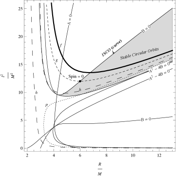
Figure 1: Region of stability of circular orbits in the $R$-$\ell^{2}$ plane.

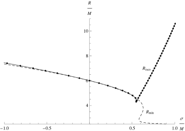
Figure 2: ISCO radius $R$ as function the spin parameter $\sigma$. The dashed line represents the values of $R$ for which the orbital angular momentum reaches its minimum.

both measured in units of $GM$. The curves labeled f, g, h represent lines of constant $\sigma$. In particular g is the curve for spinless test bodies ($\sigma=0$); it leaves the region of stability at $R=6GM$, as expected. For retrograde spin values $\sigma<0$ as represented by the curve f the ISCO is reached earlier, whilst prograde spin values $\sigma>0$ as represented by the curve h stabilize circular orbits in a range of values $R<6GM$. From these results one can infer the radial co-ordinate $R$ of the ISCO as a function of the spin parameter $\sigma$, as plotted in figure 2.

The steep line for spin values $\sigma>0.55$ has been included for completeness; here the upper limit on $B$ in inequality (66) takes over from the condition $B>0$ as the main stability criterion. However these large spin values are physically unrealistic as they can only be obtained in cases where the test-body limit is not applicable, such as binary black holes of comparable mass. Also plotted in figure 6.2 is the curve obtained by minimizing the orbital angular momentum $\ell$ as a function of $R$ at fixed spin. Cleary the two curves largely coincide.

7 Non-minimal hamiltonian dynamics of spinning test bodies

The motion of test bodies has been modeled so far using the minimal hamiltonian (14). However, it is not difficult to construct more complicated hamiltonians to model test bodies with additional interactions such as spin-curvature couplings. As the Dirac-Poisson brackets (50) are closed and model independent the equations of motion can be derived in straightforward fashion for any such extended hamiltonian. For example, one can include Stern-Gerlach type of interactions as discussed in refs. [23, 18, 20]. In this case the extended test-body hamiltonian is

$$H=\frac{1}{2m}\,g^{\mu\nu}[\xi]\,\pi_{\mu}\pi_{\nu}+\frac{\kappa}{4}\,R_{\mu\nu\kappa\lambda}[\xi]\,\Sigma^{\mu\nu}\Sigma^{\kappa\lambda}.$$ (67)

In terms of the four-velocity $u^{\mu}=\dot{\xi}^{\mu}$ the corresponding equations of motion read

$$\begin{array}[]{l}\pi_{\mu}=mg_{\mu\nu}u^{\nu},\\ \\ \displaystyle{mD_{\tau}u^{\mu}=\frac{1}{2}\,\Sigma^{\kappa\lambda}R_{\kappa\lambda\;\;\nu}^{\;\;\;\,\mu}u^{\nu}-\frac{\kappa}{4}\,\Sigma^{\kappa\lambda}\Sigma^{\rho\sigma}\nabla_{\mu}R_{\kappa\lambda\rho\sigma},}\\ \\ \displaystyle{D_{\tau}\Sigma^{\mu\nu}=-\kappa\Sigma^{\rho\sigma}\left(R_{\rho\sigma\;\;\lambda}^{\;\;\;\,\mu}\Sigma^{\lambda\nu}+R_{\rho\sigma\;\;\lambda}^{\;\;\;\,\nu}\Sigma^{\mu\lambda}\right).}\end{array}$$ (68)

As in the minimal case these equations can also be derived by requiring the vanishing of the covariant divergence of a suitable energy-momentum tensor [19]

$$\begin{array}[]{lll}T^{\mu\nu}&=&\displaystyle{T^{\mu\nu}_{min}+\frac{\kappa}{4}\,\nabla_{\kappa}\nabla_{\lambda}\,\int d\tau\left(\Sigma^{\mu\lambda}\Sigma^{\kappa\nu}+\Sigma^{\nu\lambda}\Sigma^{\mu\kappa}\right)\frac{1}{\sqrt{-g}}\,\delta^{4}(x-\xi(\tau))}\\ &&\\ &&\displaystyle{+\,\frac{\kappa}{4}\,\int d\tau\,\Sigma^{\rho\sigma}\left(R_{\rho\sigma\lambda}^{\;\;\;\;\;\,\mu}\Sigma^{\lambda\nu}+R_{\rho\sigma\lambda}^{\;\;\;\;\;\,\nu}\Sigma^{\lambda\mu}\right)\frac{1}{\sqrt{-g}}\,\delta^{4}(x-\xi(\tau)).}\end{array}$$ (69)

Here $T^{\mu\nu}_{min}$ is the energy-momentum tensor (48) of a spinning test body with minimal dynamics.

Remarkably all conservation laws for spinning bodies we derived in the minimal case carry over to the case with Stern-Gerlach interactions. In particular any constant of motion (52), (53) associated with a Killing vector $\alpha^{\mu}$ is also conserved by the Stern-Gerlach terms in the hamiltonian:

$$\frac{\kappa}{4}\,\left\{J,R_{\mu\nu\kappa\lambda}\Sigma^{\mu\nu}\Sigma^{\kappa\lambda}\right\}=0.$$ (70)

For example, in a static and spherically symmetric background like Schwarzschild or Reissner-Nordstrøm space-time the kinetic energy $E$ and the angular momentum 3-vector $\mathbb{J}$ given by equations (55) and (56) are again conserved.

This form of non-minimal hamiltonian dynamics predicts some interesting effects. In particular, as the hamiltonian is a constant of motion which by evaluation in a curvature-free region is seen to be expressed in terms of the inertial mass by $H=-m/2$, the hamiltonian constraint gets modified to read

$$g^{\mu\nu}\pi_{\mu}\pi^{\nu}+\frac{\kappa m}{2}\,R_{\mu\nu\kappa\lambda}\,\Sigma^{\mu\nu}\Sigma^{\kappa\lambda}+m^{2}=0.$$ (71)

Then the four-velocity is no longer normalized to be a time-like unit vector; instead the time-like unit vector tangent to the world line actually is

$$n^{\mu}=\frac{u^{\mu}}{\left(1+\frac{\kappa}{2m}\,R_{\mu\nu\kappa\lambda}\,\Sigma^{\mu\nu}\Sigma^{\kappa\lambda}\right)^{1/2}}.$$ (72)

Considering a particle at rest:

$$g_{tt}\left(\frac{dt}{d\tau}\right)^{2}=1+\frac{\kappa}{2m}\,R_{\mu\nu\kappa\lambda}\,\Sigma^{\mu\nu}\Sigma^{\kappa\lambda},$$ (73)

this is seen to imply that the spin-curvature coupling represents an additional source of gravitational time-dilation. A similar effect related to spinning particles interacting with electromagnetic fields was conjectured in refs. [24, 25].

8 Final remarks

The motion of test bodies carrying a finite number of relevant degrees of freedom like momentum, spin or charge can be represented by world lines in space-time to the extent that we can assign them a well-defined position and that their back reaction on space-time geometry can be neglected. Convenient position co-ordinates are not necessarily those of a center of mass (or for that matter a center of charge) in the local rest frame, as the example of spinning test bodies shows. In that case we find it preferable to associate the world line of free particles with the line on which the spin tensor is covariantly constant. The mass dipole moment can then be taken to represent the effective position of the mass with respect to that world line.

This is also clear from the corresponding energy-momentum tensor which receives contributions from both the spin proper and the mass dipole. In a next step this can be used to compute the back reaction of the test body on the space-time geometry as discussed in the simple example in section 1. In general this procedure also includes determining the self-force and the gravitational waves emitted by test bodies in the specific background under discussion [14, 26].

As another application it has been shown in the literature how the motion of test bodies can be used to reconstruct the geometry of space-time [11]. Simple geodesic motion of a sufficient number of test bodies allows one to determine the curvature at a point in space by measuring the geodesic deviations in its neighborhood. By including higher-order corrections as in eqs. (36), (37) one could also determine the derivatives of the curvature to obtain the curvature in a region around the point of interest. As equations (64) show, an alternative method is to measure first-order world-line deviations of spinning test bodies, which also depend on the gradient of the Riemann curvature tensor.

Acknowledgment
I am indebted to Richard Kerner, Roberto Collistete jr., Gideon Koekoek, Giuseppe d’Ambrosi, S. Satish Kumar and Jorinde van de Vis for pleasant and informative discussions and collaboration on various aspects of the topics discussed. This work is supported by the Foundation for Fundamental Research of Matter (FOM) in the Netherlands.

Appendix A Observer-dependence of the center of mass in relativity

To illustrate the observer-dependence of the center of mass of an extended body we consider a simple example: the motion of two equal test bodies revolving at constant angular velocity in Minkowski space on a circular orbit around an observer located in the origin of an inertial frame with cartesian co-ordinates $(t,x,y,z)$. The plane of the orbit is taken to be the $x$-$y$-plane. In fig. 3 we plot the projection of the world lines in the $x$-$t$-plane, represented by the two widely oscillating curves. At any moment the two test bodies are at equal distance to the observer and in opposite phase with respect to the origin. In this frame the center of mass is located at the origin $x=0$ and moves in a straight line along the $t$-axis in space-time.

A second observer in another inertial frame $(t^{\prime},x^{\prime},y^{\prime},z^{\prime})$ moving with constant velocity $v$ in the positive $x$-direction has a different notion of simultaneity, as defined by the appropriate Lorentz transformation. The lines $t^{\prime}=$ constant are represented by the dashed slant lines parallel to the $x^{\prime}$-axis. In the limit of large masses and slow rotation the center of mass CM^′ with respect to this moving frame is located halfway between the masses at fixed

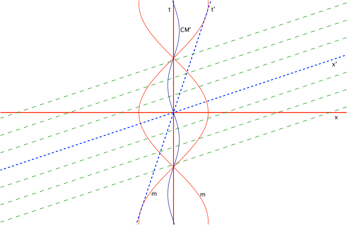
Figure 3: The world line of the center of mass of two equal masses (e.g., a binary star system) in circular orbit with respect to a stationary observer on the axis of orbital angular momentum is represented by the line $x=0$. The world line of the center of mass with respect to an observer in an inertial frame $(t^{\prime},x^{\prime})$ moving at constant velocity along the $x$-axis is represented by the oscillating curve labeled CM^′.

time $t^{\prime}$. The world line of CM^′ is now represented by the single curve oscillating at smaller amplitude around the line $x=0$ in the original frame. In fact for the observer in relative motion CM^′ moves in the negative $x^{\prime}$-direction while oscillating around the line $x^{\prime}=-vt^{\prime}$.

It is obvious that in curved space-time the notion of simultaneity is further complicated because of the non-existence of global inertial frames, resulting in additional distortions of the world line CM^′ with respect to the world line in the local inertial frame $(t,x,y,z)$ fixed to the center of rotation.

Appendix B Coefficients for geodesic deviations in
Schwarzschild geometry

The coefficients for the deviations of bound equatorial orbits w.r.t. parent circular orbits have been calculated for Schwarzschild space-time up to second order; with the restriction $\rho^{r}_{1}=\rho^{r}_{2}=0$ explained in the main text one gets the following results [6]:
a. Secular terms:

$$\begin{array}[]{ll}\rho_{1}^{t}=0,&\displaystyle{\rho_{2}^{t}=\frac{3GM}{2R^{5/2}}\frac{R+GM}{\left(R-3GM\right)^{3/2}},}\\ &\\ \rho_{1}^{\varphi}=0,&\displaystyle{\rho_{2}^{\varphi}=\frac{3}{2R^{7/2}}\sqrt{\frac{GM}{R}}\frac{\left(R-2GM\right)\left(R+GM\right)}{\left(R-3GM\right)^{3/2}}.}\end{array}$$ (74)

b. First-order periodic terms:

$$\begin{array}[]{ll}\displaystyle{n_{1}^{t}=-\sqrt{\frac{4GMR}{\left(R-2GM\right)\left(R-6GM\right)}},}&n_{2}^{t}=0,\\ &\\ \displaystyle{n_{1}^{r}=\sqrt{1-\frac{2GM}{R}},}&n_{2}^{r}=0,\\ &\\ \displaystyle{n_{1}^{\varphi}=-\frac{2}{R}\sqrt{\frac{R-2GM}{R-6GM}},}&n_{2}^{\varphi}=0.\end{array}$$ (75)

c. Second order periodic terms:

$$\begin{array}[]{l}\displaystyle{m_{2}^{t}=\sqrt{\frac{GM}{R^{2}}}\,\frac{2R^{2}-15GMR+14(GM)^{2}}{\left(R-2GM\right)\left(R-6GM\right)^{3/2}},}\\ \\ \displaystyle{m_{2}^{r}=-\frac{1}{R^{2}}\,\frac{\left(R-2GM\right)\left(R-7GM\right)}{R-6GM},}\\ \\ \displaystyle{m_{2}^{\varphi}=\frac{1}{2R^{5/2}}\,\frac{\left(R-2GM\right)\left(5R-32GM\right)}{\left(R-6GM\right)^{3/2}}.}\end{array}$$ (76)

d. Angular frequency:

$$\omega_{0}=\sqrt{\frac{GM}{R^{3}}\frac{R-6GM}{R-3GM}},\hskip 10.00002pt\omega_{1}=0.$$ (77)

In the non-restricted case with $\rho_{1}^{r}\neq 0$ also the coefficients $\rho_{1}^{t}$, $\rho_{1}^{\varphi}$, $n_{2}^{\mu}$ and $\omega_{1}$ all become non-zero as well [13].

Appendix C Coefficients for spinning world-line deviations in Schwarzschild geometry

The first-order planar deviations of circular orbits of spinning particles for constant energy and total angular momentum in Schwarzschild space-time are expressed conveniently in terms of the following combinations of orbital and spin parameters [20]

$$\begin{array}[]{ll}\alpha=\displaystyle{\frac{2(R-GM)}{R(R-2GM)}\,u^{t}-\frac{2\varepsilon}{R-2GM},}&\beta=\displaystyle{-\,\frac{GMu^{\varphi}}{mR},}\\ &\\ \gamma=\displaystyle{\frac{2R-5GM}{R(R-2GM)}\,u^{\varphi}+\frac{GM\eta}{R^{3}(R-2GM)},}&\zeta=\displaystyle{-\,\frac{GM(R-2GM)}{mR^{4}}\,u^{t},}\\ &\\ \kappa=\displaystyle{-\frac{2(R-2GM)}{R^{2}}\,\varepsilon,}&\lambda=\displaystyle{2Ru^{\varphi}-\frac{GM\eta}{R^{2}},}\\ \end{array}$$ (78)

and

$$\begin{array}[]{lll}\mu&=&\displaystyle{-\frac{2(R-3GM)}{R^{3}}+\,\frac{2(R-4GM)}{R^{3}}\,\varepsilon u^{t}+\,u^{\varphi\,2}+\frac{2GM}{R^{3}}\,\eta u^{\varphi},}\\ &&\\ \nu&=&\displaystyle{\frac{(R-GM)(R-3GM)}{R-2GM}\,mu^{\varphi}+\frac{GMm\eta}{R^{2}(R-2GM)},}\\ &&\\ \sigma&=&\displaystyle{\frac{(R-GM)(R-3GM)}{GM(R-2GM)}\,mu^{t}-\,\frac{mR\varepsilon}{GM},}\\ &&\\ \chi&=&\displaystyle{\frac{(R^{2}-4GMR+5(GM)^{2})}{GM(R-2GM)^{2}}\,mu^{\varphi}u^{t}-\,\frac{GM(3R-4GM)}{R^{3}(R-2GM)^{2}}\,m\eta u^{t}-\,\frac{m\varepsilon u^{\varphi}}{GM}.}\end{array}$$ (79)

With these definitions the frequencies of the first-order planar deviations are

$$\begin{array}[]{l}\displaystyle{\omega^{2}_{\pm}=\frac{1}{2}\left(A\pm\sqrt{A^{2}-4B}\right),}\\ \\ A=\mu-\alpha\kappa-\beta\nu-\gamma\lambda-\zeta\sigma,\\ \\ B=\beta\left(\kappa\chi-\mu\nu+\gamma(\lambda\nu-\kappa\sigma)\right)+\zeta\left(\lambda\chi-\mu\sigma-\alpha(\lambda\nu-\kappa\sigma)\right),\end{array}$$ (80)

whilst the amplitudes are given by

$$\begin{array}[]{l}n^{t}_{\pm}=\lambda(\beta\gamma-\alpha\zeta)+\beta(\omega^{2}_{\pm}-\mu),\\ \\ n^{\varphi}_{\pm}=-\kappa(\beta\gamma-\alpha\zeta)+\zeta(\omega^{2}_{\pm}-\mu),\\ \\ n^{r}_{\pm}=\omega_{\pm}(\beta\kappa+\zeta\lambda),\end{array}$$ (81)

and

$$\begin{array}[]{l}\displaystyle{N^{tr}_{\pm}=\frac{m\omega_{\pm}R^{2}}{GM}\left(1-\frac{2GM}{R}\right)n^{t}_{\pm}+\frac{2mR}{GM}\left[\left(1-\frac{GM}{R}\right)u^{t}-\varepsilon\right]n^{r}_{\pm},}\\ \\ \displaystyle{N^{r\varphi}_{\pm}=-m\omega_{\pm}Rn^{\varphi}_{\pm}-\frac{m}{R^{2}}\left(\eta+R^{2}u^{\varphi}\right)n^{r}_{\pm},}\\ \\ N^{t\varphi}_{\pm}=\omega^{2}_{\pm}(\omega_{\pm}^{2}-\mu+\alpha\kappa+\gamma\lambda).\end{array}$$ (82)

References

- [1] C. Møller. Sur la dynamique des systèmes ayant un moment angulaire interne. Ann. Inst. Henri Poincaré, 11:251, 1949.
- [2] C. Møller. The theory of Relativity. Clarendon Press, Oxford, 1952.
- [3] L. Filipe Costa and José Natário. Center of mass, spin supplementary conditions, and the momentum of spinning particles. Fund. Theories of Physics, 179:215, 2015.
- [4] S. Weinberg. Gravitation and Cosmology. J. Wiley, N.Y., 1972.
- [5] E. Hackmann. Geodesic equations and algebro-geometric methods. arXiv:1506.00804v1 [gr–qc], 2015.
- [6] R. Kerner, J.W. van Holten, and R. Collistete jr. Relativistic epicycles: another approach to geodesic deviations. Class. Quantum Grav., 18:4725, 2001.
- [7] R. Colistete Jr., C. Leygnac, and R. Kerner. Higher-order geodesic deviations applied to the Kerr metric. Class. Quantum Grav., 19:4573, 2002.
- [8] J. Ehlers, F.A.E. Pirani, and A. Schild. The geometry of free fall and light propagation; in: General Relativity: Papers in Honnor of J.L. Synge, ed. L. O’Raifeartaigh. Oxford Univ. Press, 1972.
- [9] C.W. Misner, K.S. Thorne, and J.A. Wheeler. Gravitation. Freeman and Co., San Francisco, 1970.
- [10] P. Szekeres. The gravitational compass. J. Math. Phys., 6:1387, 1965.
- [11] D. Puetzfeld and Y.N. Obukhov. Generalized deviation equation and determination of the curvature in General Relativity. Phys. Rev., D93:044073, 2016.
- [12] D. Philipp, D. Puetzfeld, and C. Lämmerzahl. On the applicability of the geodesic deviation equation in General Relativity. arXiv:1604.07173 [gr–qc], 2016.
- [13] G. Koekoek and J.W. van Holten. Epicycles and Poincaré Resonances in General Relativity. Phys. Rev., D83:064041, 2011.
- [14] G. Koekoek and J.W. van Holten. Geodesic deviations: modeling extreme mass-ratio systems and their gravitational waves. Class. Quantum Grav., 28:225022, 2011.
- [15] M. Mathison. Neue Mechanik materieller Systeme. Acta Phys. Polon., 6:163, 1937.
- [16] W. Tulczyjew. Motion of multipole particles in General Relativity theory. Acta Phys. Pol., 18:393, 1959.
- [17] J. Steinhoff. Canonical Formulation of Spin in General Relativity. Ph.D. Thesis, (Jena Univ.); arXiv:1106.4203v1 [gr-qc], 2011.
- [18] G. d’Ambrosi, S. Satish Kumar, and J.W. van Holten. Covariant hamiltonian spin dynamics in curved space-time. Phys. Lett., B 743:478, 2015.
- [19] J.W. van Holten. Spinning bodies in general relativity. Int. J. of Geometric Methods in Modern Physics, 13:1640002, 2016.
- [20] G. d’Ambrosi, S. Satish Kumar, J.W. van Holten, and J. van de Vis. Spinning bodies in curved space-time. Phys. Rev., D93:04451, 2016.
- [21] J. Ehlers and E. Rudolph. Dynamics of extended bodies in general relativity: Center-of-mass description and quasi-rigidity. Gen. Rel. Grav., 8:197, 1977.
- [22] R. Ruediger. Conserved quantities of spinning test particles in General Relativity. Proc. Roy. Soc. London, A375:185, 1981.
- [23] I. Khriplovich and A. Pomeransky. Equations of motion for spinning relativistic particle in external fields. Surveys High En. Phys., 14:145, 1999.
- [24] J.W. van Holten. On the electrodynamics of spinning particles. Nucl. Phys., B356, 1991.
- [25] J.W. van Holten. Relativistic time dilation in an external field. Physica, A 182:279, 1992.
- [26] G. d’Ambrosi and J.W. van Holten. Ballistic orbits in Schwarzschild space-time and gravitational waves from EMR binary mergers. Class. Quantum Grav., 32:015012, 2015.