Pre-nebular Light curves of Type I supernovae

Abstract

We compare analytic predictions of supernova light curves with recent high quality data from SN2011fe (Ia), from KSN2011b (Ia), and the Palomar Transient Factory (PTF) and the La Silla-QUEST variability survey (LSQ) (Ia). Because of the steady, fast cadence of observations, KSN2011b provides unique new information on SNe Ia: the smoothness of the light curve, which is consistent with significant large-scale mixing during the explosion, possibly due to 3D effects (e.g., Rayleigh-Taylor instabilities), and provides support for a slowly-varying leakage (mean opacity). For a more complex light curve (SN2008D, SNIb), we separate the luminosity due to multiple causes and indicate the possibility of a radioactive plume. The early rise in luminosity is shown to be affected by the opacity (leakage rate) for thermal and non-thermal radiation. A general derivation of Arnett’s rule again shows that it depends upon all processes heating the plasma, not just radioactive ones, so that SNe Ia will differ from SNe Ibc if the latter have multiple heating processes.

DRAFT FROM

1 Introduction

Supernovae whose luminosity is primarily powered by the decay chains $\rm{}^{56}Ni(e^{-},\nu){{}^{56}Co}$, $\rm{}^{56}Co(e^{-},\nu){{}^{56}Fe}$ and $\rm{}^{56}Co(,e^{+}\nu){{}^{56}Fe}$ have generic features. These are prominent in SNe Ia, and appear in SNe Ibc, that is, in both thermonuclear supernovae and those core-collapse supernovae which have lost their hydrogen envelopes (e.g., Arnett (1982, 1996)).

We compare theoretical light curves (Arnett, 1982; Pinto & Eastman, 2000a, b) to the best-observed typical SN Ia to date, SN2011fe in M101, the Pinwheel galaxy (Pereira, et al., 2013), as well as to KSN2011b, the best of three SNe Ia (KSN2011b,c; KSN2012a) detected at early times by the Kepler satellite (Olling, et al., 2015). For these supernovae we have bolometric (or near bolometric) light curves, so we may minimize issues of frequency-dependent atmospheric physics. This approach, which assumes three–dimensional (3D) incomplete mixing during the explosion (Arnett & Meakin, 2016), is thus different from and a natural complement to a 1D, time–dependent stellar atmosphere approach such as Blondin, et al. (2013); Dessart, et al. (2015, 2016).

In §2 we introduce the combined problem of parameters and uniqueness, which may be more clearly discused in our analytic framework. In §3 we discuss SN2011fe, including the early light curve. In §4 we discuss leakage of thermal and non-thermal radiation from supernovae in terms of an effective opacity. In §5 we discuss KSN2011b, the problem of converting it to a bolometric scale, and show that it has an exceptionally smooth light curve, constraining theoretical models of mixing. In §6 we present a more general derivation of Arnett’s rule (Arnett, 1979, 1982). In §7 we discuss the core-collapse SN2008D (type Ib), and separate the breakout, shock, and radioactive heating parts of the light curve. §8 contains our summary.

2 Uniqueness

Light curves of Type I supernovae have a characteristic shape which is due to radioactive heating by gamma-rays and positrons, cooling by expansion, and cooling by radiative loss (Arnett, 1982; Pinto & Eastman, 2000a). The shape of these light curves is determined by a parameter

$$y=(2\tau_{d}\tau_{h})^{1\over 2}/2\tau_{Ni}\sim(\kappa_{t}M_{ej}/v_{sc})^{1\over 2},$$ (1)

which is a combination of diffusion time and expansion time, relative to the a reference time (the decay time for $\rm{}^{56}Ni$), or equivalently the effective opacity times mass ejected divided by the velocity scale. The amplitude (peak light) is determined by

$$L = \epsilon_{Ni}M_{Ni}M_{\odot}\Lambda(x,y)$$ (2)

$$= 2.055\times 10^{10}L_{\odot}M_{Ni}\Lambda(x,y)$$

where the dimensionless function $\Lambda$ is determined by an integration in time, and $M_{Ni}$ is the mass of ⁵⁶Ni in solar units. An estimate of radioactive heating by a mass $M_{Ni}$ at peak light requires an estimate of the time between explosion (synthesis) and peak light. The theory is not a one-zone model as in Arnett (1979), but involves integration over both space and time by separation of these variables (see Arnett (1982), Eq. 11 and 48).

The light curves are determined by five astrophysical parameters, acting in combination (Eq. 1 and Eq. 2). They are the mass ejected $M_{ej}$, the mass of $\rm{}^{56}Ni$ ejected $M_{Ni}$, the initial radius $R(0)$, the effective opacity $\kappa_{t}$ (a measure of leakage rate for radiant energy, see §4), and the explosion energy $E_{sn}$. The initial radius of the white dwarf is $R(0)\ll 10^{13}$ cm so that its precise value is unimportant for the light curve. If the remaining four parameters are constrained to be consistent with a thermonuclear explosion of a white dwarf, realistic light curves for SNe Ia result.

The situation is more complex for SNe Ibc: (1) there is a collapsed remnant which may be active, and (2) there may be fluid dynamic heating due to interaction of the ejecta with a mantle or any surrounding gas, for example.

This additional physics may imply new parameters, further adding to the problem of uniqueness. If we infer $y$ from the shape of the light curve, this only fixes the combination $\kappa_{t}M_{ej}/v_{sc}$ (not the individual values, for which additional constraints are needed). It might be a good project to examine spectral estimates of velocity to constrain velocity structure, for example. So far this seems to have been done using $v(t)$, which maps into radius $v(r)$ easily enough, but not mass coordinate $v(m)$ with any precision. That is required because $E_{KE}=0.3v_{sc}^{2}/M_{ej}$.

3 Light curves for SN2011fe

Because the theoretical models preceded the acquisition of high quality data by decades, and the physical parameters are nearly the same now as then (cf. Table 1), the models are a prediction in this sense. It is easy to capture the observed behavior with these theoretical models. Fig. 1 illustrates this observationally for SN2011fe (Pereira, et al., 2013) using (Arnett, 1982).

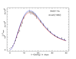
Figure 1: Comparison of bolometric luminosity from analytic models (Arnett, 1982) and from SN2011fe (Pereira, et al., 2013). The analytic models plotted here allow for $\gamma$–ray escape, as did the original ones, by using the deposition estimate from Monte Carlo simulations of Colgate, Petschek & Kriese (1980). The three curves are distinguished by a slightly different value for the mass of $\rm{}^{56}Ni$, $M_{Ni}=0.546\pm 0.016M_{\odot}$, which agrees well with that inferred by Pereira, et al. (2013); see text and Table 1. The peak luminosity increases with $M_{Ni}$.

We consider the original case of massive CO white dwarfs igniting $\rm{}^{12}C$ under conditions of high electron degeneracy as being appropriate to SN2011fe and KSN2011B; see Nugent, et al. (2011) for observational support. Burning ¹²C and ¹⁶O to nuclei lying in the range ²⁸Si–⁴⁰Ca releases almost as much explosive energy as burning the same nuclei to ⁵⁶Ni ($q_{SiCa}\sim q_{Ni}$), but the ashes (Si–Ca) are not radioactive, and do not provide late heating. We adjust the Ni production to fit the peak luminosity. We assume that comparable amounts of Si–Ca and Ni are produced, which determines the explosion energy. We adjust the effective opacity to fit the shape of the light curve. The values chosen for SN2011fe light are documented in Table 1.

Table 1: Base model for SN2011fe

Symbol	Fig. 1	A82a
$M_{ej}$b ($M_{\odot}$)	$1.40$	$1.45$
$M_{Ni}(0)$c($M_{\odot}$)	$0.546\pm 0.016$	0.5—0.7
$R(0)$	$4.0\times 10^{8}$ cm	0—$10^{13}$ cm
$\kappa_{t}$ ( cm2 g-1)	$0.09$	0.08 — 0.1
$E_{sn}$ ($10^{51}\rm\,erg$)	1.2	$\sim 1$
$y^{2}$	$0.573$	0.8 — 1.2

With a mass of $\rm{}^{56}Ni$ of $0.546M_{\odot}$, after 14.14 days (but see §3.1) a maximum luminosity of $3.00\times 10^{9}\,L_{\odot}$ is reached; which fits the data of Pereira, et al. (2013), who quote $3.04\times 10^{9}\,L_{\odot}$. They use $M_{Ni}=(0.44\pm 0.08\times(1.2/\alpha)M_{\odot}$, with $\alpha=1.2$ to infer the mass of $\rm{}^{56}Ni$; this expression is from Gonzalez-Gaitán, et al. (2012) and has assumptions regarding three-dimensional (3D) effects (see Arnett & Meakin (2016) for a discussion of 3D and resolution issues). We prefer to take $\alpha=1$ so that the observationally inferred value is $M_{Ni}=0.528\pm 0.08M_{\odot}$, which agrees better with the actual 3D simulations of Röpke, et al. (2012), who found $M_{Ni}\sim 0.61M_{\odot}$.

At peak only $83.8$ percent of the instantaneous radioactive energy release is being deposited in our model, while the rest escapes as x-rays and gamma-rays rather than as thermalized radiation. The mass fractions of $\rm{}^{56}Ni$ and $\rm{}^{56}Co$ are $0.197$ and $0.741$ respectively. Decays of $\rm{}^{55}Co$ and $\rm{}^{57}Ni$ have a negligible effect of this part of the light curve.

Table 2: Some Initial^a values

Variable	Symbol	Value
Velocity scale	$v_{sc}$	$9.28\times 10^{8}$ cm s-1
Hydro time	$\tau_{h}$	$0.43$ s
Diffusion time	$\tau_{d}$	$1.52\times 10^{12}$ s
Central Density	$\rho(0,0)^{b}$	$1.04\times 10^{7}$ g cm-3
Central Temperature	$T(0,0)$	$8.77\times 10^{8}$ K
Optical depth	$\tau_{t}(0)$	$3.73\times 10^{14}$

Table 2 gives some initial values constructed from these parameters. The initial radius divided by the velocity scale gives an expansion time scale $\tau_{h}\sim 4\times 10^{8}/10^{9}\sim 0.4$ s. The diffusion time for photons is larger, $\tau_{d}\sim 1.5\times 10^{12}$ s. This implies that an enormous expansion must occur before photons leak out readily, and that the temperature is determined by a balance between adiabatic cooling and radioactive heating. After the explosion, the Hugoniot-Rankine relations for a shock wave imply that the enthalpy and kinetic energy are comparable. Spherical expansion will reduce the internal energy by a factor $\tau_{h}/t$, so that within a minute the internal energy is reduced to $1.2\times 10^{-4}$ of its post shock value. This energy is converted into kinetic energy by work done by pressure in expanding the matter, ${3\over 10}M_{ej}v_{sc}^{2}\rightarrow E_{sn}$, and we have an expanding Hubble flow. The energy released by radioactive decay equals the reduced thermal energy after about $40$ s; after that the internal energy results from radioactivity. “Early” observations ($t>$ 1 hour) of SNe Ia tell us primarily about thermal, not hydrodynamic effects.

This implies that (after 1 hour) the spatial distribution of internal energy closely tracks that of radioactivity, because that internal energy is caused by radioactive heating. This resolves an issue in Arnett (1982), Eq. 13, in which this was assumed without justification.

At much later times, $t\sim 10^{15}{\,\rm cm}/v_{sc}\sim 10^{6}$ s, maximum light occurs, with thermal photons, x-rays and $\gamma$-rays leaking rapidly.

3.1 Early time light curve

Figure 1 shows an excellent agreement of the original theory with observations. However the new data offer the promise of new understanding: the first three data points are higher than the theoretical ones. In reality the opacity is not constant as assumed; at early times the temperature and density are rapidly changing, on a time scale $t\sim R(t)/v_{sc}$, so variations in opacity are plausible.

Given Eq. 2, and expanding $\Lambda(x,y)$ at early times ($t/\tau_{Ni}=xy\ll 1$), we have $\Lambda(x,y)\rightarrow x^{2}$ (Eq. 45 in Arnett (1982)). The normalized luminosity is then

$$L/\epsilon_{Ni}M_{Ni}=t^{2}/(2y\tau_{Ni})^{2},$$ (3)

which is the same form used by Firth, et al. (2015) but with $n=2$ and $a=1/(2y\tau_{Ni})^{2}$. If $y^{2}=(\tau_{d}\tau_{h}/2\tau_{Ni}^{2})\propto\kappa_{t}M_{ej}/v_{sc}$, is not strictly constant, but decreases slowly with time, $n>2$ results. Such a decrease in opacity is also needed to make the light curve in Fig. 2 merge into that in Fig. 1 at peak luminosity.

This differs from the more limited “blast wave” approximation usually used to support a $t^{-2}$ behavior: here the effective temperature $T_{eff}$ and the velocity at the photosphere $v_{photos}$ are not required to be constant. They are only constrained to radiate the luminosity leaked from inside.

Nugent, et al. (2011) found the initial rise of SN2011fe to be well-described by a radiative diffusion wave with an opacity due to Thomson scattering, $\kappa=\kappa_{th}$; Figure 2 confirms this, using the parameter values of Table 1, but increasing $\kappa\rightarrow\kappa_{th}\approx 0.2\,\rm cm^{2}\,g^{-1}$. Now the earliest three points lie on the theoretical curve, but the luminosity in the peak is too low because the opacity is too high; $\kappa\sim 0.09\rm\,cm^{2}\,g^{-1}$ at peak is needed to model the escape of thermal energy. At later times ($t>30$ days after explosion) the shape of the light curve is controlled by increasing gamma-ray escape, and the numerical value of the effective opacity for thermal radiation is not so important.

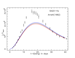
Figure 2: Comparison bolometric luminosity from analytic models (Arnett, 1982) and SN2011fe (Pereira, et al., 2013). Here the effective opacity is $\kappa_{t}=0.2\,\rm cm^{2}g^{-1}$, appropriate for early times when Thompson scattering dominates. The early points ($t<6$ days) agree with the analysis of Nugent, et al. (2011), but bang time is about 2 days earlier than in Fig. 1. After about 8 days the analytic model has an effective opacity which is too large around peak light ($\kappa_{t}=0.2>0.09\,\rm cm^{2}g^{-1}$), but at 30 days after explosion, with gamma-escape important, the light curve again approaches the observed values again.

The “bang time” (time of explosion) in Figure 2 is now earlier by 2 days. Firth, et al. (2015) found a rise time of $18.98\pm 0.54$ days for 18 SNe Ia, ranging from $15.98$ to $24.7$ days. For SN2011fe our value of $14.14+2\sim 16.1$ days agrees well with the Pereira, et al. (2013) value of $16.58\pm 0.14$ days.

Firth, et al. (2015) find the exponent of the power law fit to the early rise to be $n=2.44\pm 0.13$. Although Figure 2 begins as $L\propto t^{2}$, merging upward to Figure 1 requires an steeper increase in the transition and thus $n>2$ if a power-law fit is made for constant $a$ (i.e., $L\approx a\,t^{n}$).

We note that this behavior of $n$ may be a general property of the decoupling of super-thermal photons with continuing expansion rather than the distribution of $\rm{}^{56}Ni$, as suggested by Piro & Nakar (2013), or a combination of the two. It remains to disentangle these effects; they both deal with the effects of radioactive decay heating.

3.2 Opacity

Consider a simple leaky-bucket model for radiation loss; frequency regions of low opacity are “holes” and determine the leakage rate. The highest energy photons (gamma and x-rays) have their longest mean-free paths for scattering, and these interactions fill the holes because of their relatively weak frequency dependence (see §4.3). At early times the gamma and x-rays are downscattered into the thermal range, so the the relevant scattering cross section for filling the holes is that for Thomson scattering, and $\kappa_{th}=0.20\rm\,cm^{2}\,g^{-1}$. At late times a floor on the opacity is derived from the Klein-Nishina transport cross section to be $\kappa_{KN}=0.067\rm\,cm^{2}\,g^{-1}=\kappa_{th}/3$. Fitting the shape of the peak in Figure 1 gave us $\kappa_{t}\approx 0.09\rm\,cm^{2}\,g^{-1}$ which lies between these limits. Apparently the effective opacities for energy leakage in SNe Ia are (1) small, (2) vary little, ($0.067<\kappa_{t}<0.2$), and (3) are insensitive to composition, a surprising result given the complexity of the spectra and the problem. This is consistent with the discussion in Dessart, et al. (2014), §3.2. It seems that leakage of energy rather than line formation is the key issue for bolometric light curves; spectra are the opposite.

It appears that a modest and plausible variation in the effective opacity (escape probability) will allow an excellent description of the SN2011fe light curve, e.g., something like Figure 1 with Figure 2 for the first few days would result from a slowly varying (almost constant) opacity.

4 Opacity and Energy Leakage

In Section 3 we found that the effective opacity to be the remaining parameter, from the original five, which needed to be used to adjust the light curves to fit the data from SN2011fe. The analytic solutions for the bolometric light curve require a rate at which photon energy, both thermal and non-thermal, leaks from the ejected mass; this may be quantified by a “leakage time”.

4.1 Leakage time

The thermal leakage is estimated by a radiative diffusion model, which involves the integrated effect of the opacity over the structure and time (Arnett, 1982; Pinto & Eastman, 2000a, b, c). Although the local opacity will vary sensitively with the local density, temperature and photon frequency, the leakage time integrates these effects over a dynamic structure (Pinto & Eastman, 2000b), giving a smoother variation in global properties. The term “opacity” in the analytic solutions is a placeholder for a leakage time. This “effective opacity” was taken to be a constant (for analytic simplicity) which approximates the same leakage of radiative energy as a physically correct simulation would (in practice, this may only mean that the choice of effective opacity fits the observations).

As seen above, this should include effects due to x-ray and $\gamma$-ray transport, not just deposition as in Colgate, Petschek & Kriese (1980). As maximum light is approached, energy transport by superthermal photons (x-rays and $\gamma$-rays) becomes comparable to that by “thermal photons” (see Pinto & Eastman (2000b) for discussion of thermalization). As maximum light is approached non-thermal heating becomes less localized and mean-free-paths become longer. If we regard this as a second channel for energy flow, the effective opacity would be (roughly) the inverse average over both thermal and non-thermal channels, with the lower opacity channel carrying more energy.

4.2 Conditions at maximum light

Table 3 shows the values of selected variables at maximum light for the models presented in Figure 1. The temperatures lie in the range $1\times 10^{4}$ K to $2\times 10^{4}$ K, which are commonly found in normal stars. Due to the large radiative conductivity, the SN has a relatively shallow temperature gradient.

Unlike the temperatures, the densities (of order $3\times 10^{-13}$ g cm^-3) are considerably lower than encountered in stellar atmospheres. These low densities suggest the question: how valid is the assumption of collisional equilibrium? As discussed in Pinto & Eastman (2000b), thermal velocity $v\ll c$ implies that collisional equilibrium is difficult to attain in supernovae, and thermal equilibrium comes from radiative interactions.

Table 3: Variables at Peak Light^a

variable	value
$t_{max}-t_{bang}$	14.14 daysb
$L_{max}$	$3.00\times 10^{9}\,L_{\odot}$
m(bol)	-18.97
$\rho_{c}$	$4.56\times 10^{-13}\,\rm g\,cm^{-3}$
$T_{c}$	$1.92\times 10^{4}\rm\,K$
$T_{eff}$	$1.06\times 10^{4}\rm\,K$
$\tau_{h\nu}$(thermal)	46.6
$\tau_{\gamma}$(superthermal)	15.5
D($\gamma$-deposit)	$0.838$
56Ni	$0.199$
56Co	$0.740$
57Ni	$3.12\times 10^{-5}$
57Co	$0.0237$

4.3 LTE Fe opacities and holes

Chris Fontes has calculated new LTE opacities for these low densities, which are shown in Figure 3. These opacities are produced by the OPLIB database team (Magee et al., 1995) with new calculations for the low densities needed for light-curve calculations, and shown in Fig. 3. Following Pinto & Eastman (2000b) we accept that LTE is a flawed approximation in detail, but use it to suggest qualitative behavior. In a simplified leakage scheme for transport of energy, we assume a single opacity for the transport, but the opacities vary dramatically with photon energy. For leakage schemes, the transport is dominated by the dips in the opacity, not the peaks. The energy where this dip occurs depends both on the temperature and density of the supernova ejecta, and the leakage opacity may vary both up and down as the ejecta expand, ranging within the visible bands from below $0.001\rm\,cm^{2}\,g^{-1}$ to above $10\,\rm\,cm^{2}\,g^{-1}$.

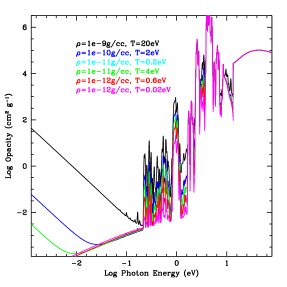
Figure 3: Logarithm of Fe opacity as a function of photon energy for various combinations of density and temperature using an extension of the OPLIB database (Magee et al., 1995) (courtesy Chris Fontes). Note that as the ejecta expands (and the density and temperature decrease), the opacity in a given band can both decrease and increase. At low density ($\rho=10^{-12}\rm\,g\,cm^{-3}$) gaps open in the atomic opacity, which decreases toward the IR frequencies.

As the densities approach supernova values ($\rho<10^{-12}\rm\,g\,cm^{-3}$), the opacity in Fig. 3 shows gaps with values $\log_{10}\kappa\sim-2$, around and below the LTE temperature of 1eV. Guided by Pinto & Eastman (2000b) we assume that this property is set by atomic structure and will be qualitatively true for non-LTE distributions of states; see also Dessart, et al. (2014, 2015, 2016), who find that their spectra are surprisingly insensitive to the opacity controling the radiation flow.

Non-thermal radiation may affect the degree of ionization around peak light, when thermalization is weakening, and affect the leakage and transport of energy. Such effects have been subsumed in the ”effective opacity”.

This appears to support the inference from §3 that the effective opacity may be controlled by scattering processes, Thomson and Compton, which close leaks.

4.4 Leakage and transport

To better understand the effect of such opacities, we have implemented an opacity switch in the simplified transport code of Bayless, et al. (2013) that allows the opacity to move up or down by an order of magnitude as the temperature drops below 1 eV ($1.16\times 10^{4}$ K). Figure 4 shows the light curves from a standard model assuming $\kappa=0.1$ as well as the opacity switch that increases and decreases the opacity. These light-curves demonstrate the sensitivity to opacity. With a full transport solution, we might expect opacity variation to produce observable features in the light curve (which we do see), but the basic trends with the slopes will not change dramatically. Notice that for the increased opacity case, the lightcurve begins to rise earlier, as in Figure 2.

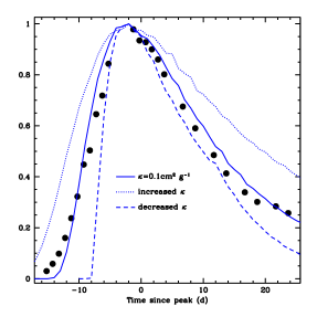
Figure 4: Comparison of bolometric luminosity from SN2011fe (Pereira, et al., 2013) (solid dots) using our diffusion code with three opacity prescriptions: (a) constant $\kappa=0.1\rm\,cm^{2}\,g^{-1}$ (solid), (b) increase at low temperatures: $\kappa$ increases to $1\rm\,cm^{2}\,g^{-1}$ below 1 eV (dotted), and (c) decrease at low temperatures: $\kappa$ decreases to $0.01\rm\,cm^{2}\,g^{-1}$ below 1 eV (dashed). Increasing the opacity broadens the light-curve, decreasing narrows it. These explosions assume an explosion mass of $1.4\,{\rm M}_{\odot}$, an explosion energy of $1.3\times 10^{51}\,{\rm erg}$ and a nickel mass of $0.6\,$M_⊙

Until these issues are convincingly resolved, the leakage time should be considered an adjustable parameter, strongly constrained by observation, constrained less strongly by microscopic theory, but not yet one solidly founded in experiment and simulation.

4.5 Filaments and mixing

In addition to issues associated with line formation and leakage, there are the difficulties associated with non–spherical variation inevitably resulting from instabilities in the explosion. Theoretical models of supernovae which are spherically symmetric have no angular resolution to deal with this broken symmetry. Mixing is treated in a ad-hoc manner. Observed young supernova remnants have a pronounced filamentary structure, a heterogeneity which may have developed during this epoch of instability.

How might this happen? We summarize the discussion in Arnett & Meakin (2016) and Arnett, et al. (2015). Explosions are rife with instabilities. Most notable are Rayleigh-Taylor and Richtmeyer-Meshkov instabilities, which also appear in simulations of convection by bottom heating. Heat gives rise to plumes which develop a mushroom cloud shape. In a convective region the upward motion is bounded and turned back. Because of the astronomically large Reynolds number, the flow is turbulent and gives rapid mixing, which in high-resolution simulations is essentially complete in two turn-over times (four transit times). Suppose the heating is violent, and the motion is not contained (an explosion). Then only one transit time is available for mixing, which is global yet incomplete. Turbulence is frozen by expansion. A fundamental feature of turbulence is high vorticity: vortex filaments are the “sinews” of turbulence (Landau & Lifshitz, 1959; Pope, 2000). Further expansion of the supernova may lead to a regime of thermal instability, in which denser regions radiate, cool, and are further compressed, leaving the sort of filamentary structure seen in young supernova remnants. Is it possible to test this idea with observations of supernova light curves? The Kepler observations of supernovae may bear on this question.

5 Supernova KSN2011B

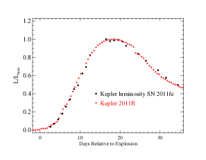
Figure 5: Comparison of Kepler-normalized luminosities (i.e., in the Kepler filter bandpass) for SN2011fe and KSN2011b (Olling, et al., 2015). When normalized at peak light the two SNe Ia look very similar. The time axis was translated to match the point of explosion. We took the time of explosion for SN 2011fe from Pereira, et al. (2013) (2.6 days before the first spectrum) and from Olling, et al. (2015) for Kepler 2011b (18.1 days before maximum).

While the Kepler satellite does not have wavelength coverage comparable to that which became available for SN2011fe, the Kepler coverage is broadband, has high cadence in time, has small errors from statistical fluctuations, and the light curves track the data from SN2011fe well; see Fig. 1 in Olling, et al. (2015). We suggest that the Kepler data provide a constraint on mixing in SNe Ia that is unattainable even with the high quality UVOIR data available for SN2011fe.

The spectra of SN 2011fe in Pereira, et al. (2013) were obtained using the SuperNova Integral Field Spectrograph (Lantz et al., 2004) on the 88” telescope on Mauna Kea and are presented as fully calibrated. We multiplied the spectra by the filter function for Kepler (a wide filter, $\sim 4400-8800$ A). The Kepler system is not fully calibrated, so there is no measured zero point to place Kepler magnitudes onto a known scale. We used a zero point similar to that for standard filters, a procedure which gives a reasonable answer, but still contains some arbitrary scaling. Even evaluating the flux directly from the spectra through the filter requires some knowledge of the calibration of the filter. We can construct a Kepler magnitude and a flux in the Kepler filter for each spectrum that are all consistent relative to each other, but there is still an uncertain absolute scaling. Actual bolometric corrections are hard to do without calibrating the Kepler system.

It appears that SN2011fe and KSN2011b are similar enough (Fig. 5) that we may use this similarity in the data to establish a correspondence between the bolometric scale of SN2011fe and the Kepler supernovae.

5.1 A Calibration

From Fig. 5, we infer that the bolometric light curve of KSN2011b would be similar to SN2011fe. There are many caveats that need to be considered for such an inference, such as the fact that SN2011fe and KSN2011b may have different bolometric characteristics. Given the striking similarity of the two light curves in the Kepler band, though, we believe that this is a plausible inference. Using the bolometric luminosties from Pereira, et al. (2013), we establish a ‘bolometric correction’ for our derived Kepler-magnitude light curve of SN 2011fe. We then apply the same corrections to KSN2011b to derive a bolometric light curve. We take the flux and treat it as a relative luminosity (L/L_max); this ratio also removes concerns about absolute scaling. Fig. 6 shows the time evolution of the bolometric L/L_max for both SN2011fe and KSN2011b.

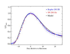
Figure 6: Comparison of the bolometric luminosity of SN 2011fe (Pereira, et al., 2013) and adjusted data (see text) based on KSN2011b (Olling, et al., 2015). The light curves presented by Pereira, et al. (2013) are also obtained by convolving filter functions with their spectra. They estimate the errors in their magnitudes using the flux calibration procedure for their spectra and we adopt the same 1$\sigma$ errors per epoch. The errors for KSN2011b incorporate those errors as the bolometric correction is applied. The choice of explosion time (the precise zero of the x-axis) depends upon the algorithm used, and may be uncertain by a day or so (see §3.1).

Now that we have a calibration, how does the best Kepler supernova compare with the analytic curves? KSN2011b, from Olling, et al. (2015) is shown in Fig. 6. Random photometric errors of KSN2011b are small. The uncertainties in the SN 2011fe bolometric luminosities and the bolometric corrections applied to the KSN2011b Kepler magnitudes dominate the error bars. There is evidence for a well-defined and smooth light curve, but systematic biases might affect details of shape fitting.

Again we see a deviation between observations and analytic light curves at very early times, which we attribute to use of a constant effective opacity. After this first deviation, the curves are strikingly similar, as the higher cadence of the Kepler data makes clear. Although the observed supernovae might not be identical, so that fitting with different theoretical parameters would be legitimate in principle, we have used exactly the same theoretical parameters as in Fig. 1 in order to illustrate just how similar these light curves seem to be.

Because of the steady, fast cadence of observations, KSN2011b provides unique new information on SNe Ia: the smoothness of the light curve. While KSN2011b tracks SN2011fe within its error bars, the KSN2011b light curve is noticeably smoother. There is no indication of any bumps due to collision of ejecta with circum-supernova matter, as with type Ibn and IIn events. The smoothness of 1D theoretical light curves result from ad-hoc “box-car” mixing; simulations without such mixing are not smooth (Pinto & Eastman, 2000a; Dessart, et al., 2015, 2016). Explosions are unstable to 3D mixing which can leave an imprint on the young supernova remnant as well as the light curve (Arnett & Meakin, 2016). SN2011fe does exhibit larger fluctuations in its light curve, consistent with its observational error bars.

6 Arnett’s rule

It has been shown, for one-zone models (Arnett, 1979), with constant opacity and radioactive heating by ⁵⁶Ni and ⁵⁶Co decay, that

$$L_{peak}/M_{ej}\approx\epsilon_{NiCo}(t_{peak}).$$ (4)

where $L_{peak}$ is the luminosity at maximum light, $M_{ej}$ is the ejected mass, and $\epsilon_{NiCo}(t_{peak})$ is the instantaneous rate of energy production from radioactivity at that time. From a solution by separation of variables (radius and time), a more accurate expression was derived,

$$L_{peak}/M_{ej}=\epsilon_{NiCo}(t_{peak})D,$$ (5)

where $D$ is the deposition function of Colgate, Petschek & Kriese (1980), which is a function of “optical” depth for $\gamma$-rays (see § IV.a in Arnett (1982)). For SN2011fe, $D=0.838$ at maximum light (Fig. 1), which corresponds to a correction to Eq. 4 of $\approx 20$ percent (increase) in estimated radioactive mass.

6.1 A Derivation

Here we present a new derivation which is more concise, general, and hopefully clearer. We emphasize that, as in Arnett (1982), it is the instantaneous total heating rate of the plasma which is constrained, not the radioactive decay rate, which may explain at least part of the discrepancy with Dessart, et al. (2015, 2016). In addition we add a brief appendix summarizing a modern approach to solving for Arnett (1982) light curves, so that errors in implementation may be easily corrected.

The luminosity due to radiative diffusion may be written as

$$L=aT^{4}R^{3}/\tau_{dif},$$ (6)

where

$$\tau_{dif}\sim\kappa M/\beta cR,$$ (7)

and $\beta\approx 13.7$ is a dimensionless form factor from integration of the diffusion equation over space. It includes the geometric factor for spherical geometry, and is very slowly varying with mass-density structure; see Arnett (1980), Table 2 and §VI.

At any extremum in $L$, either a peak or a dip, $dL/dt=0$. The time derivative of Eq. 6 is

$$d\ln L/dt = 4d\ln T/dt+4d\ln R/dt$$ (8)

$$- d\ln\kappa/dt.$$

For a slowly-varying escape time, the term $d\ln\kappa/dt$ will be small; see discussion in §4. This is also consistent with the good fits to the light-curve data shown in Fig. 1.

A second equation involving the luminosity is first law of thermodynamics, which may be written after spatial integration as

$$L/M\sim\epsilon(t)D-dE/dt-PdV/dt.$$ (9)

For homologous expansion (Hubble flow)

$$d\ln V/dt=3d\ln R/dt$$

and for a radiation-dominated plasma,

$$E=3PV=aT^{4}V,$$

so

$$dE/dt+PdV/dt=E(4d\ln T/dt+4d\ln R/dt).$$ (10)

This requires a 3D simulation of high resolution to compute accurately (Arnett & Meakin, 2016), but deviations from Hubble flow may be thought of as compressional heating and expansional cooling from an inelastic collision within the supernova ejecta (Arnett (1980), § VIII), or with surrounding matter (Smith, 2017). Using Eq. 8 and 10 we have

$$L/M\sim\epsilon(t)D-E(d\ln L/dt+d\ln\kappa/dt).$$ (11)

At any extremum in $L$, $dL/dt=0$, so at that time we have

$$L/M=\epsilon D-E\,d\ln\kappa/dt,$$ (12)

for any plasma heating rate $\epsilon D$. This will be true at multiple peaks and at dips as well. This is a more general form of Eq. 5.

As emphasized in Arnett (1982) SNe Ia are special in that the kinetic energy source and synthesis of radioactivity are more directly linked than in SNe Ibc. Heating from other causes would have the same qualitative effects as radioactive heating. The $\epsilon D$ in Eq. 12 may be generalized to be the sum of all processes heating the ejecta. It may be affected by relativistic jets (the fraction of their energy which is thermalized), magnetars, pulsars, fluid accretion (fall-back) onto a neutron star, and so on, as well as radioactivity. SNe Ia models are simple in that they have only one heating source and no collapsed remnant.

In Fig. 1 there are two extrema in luminosity: at the time of explosion (bang time) and at maximum light. The first peak at very early time is due to shock breakout, and occurs at such small radii that it has negligible effect on the luminosity for SNe Ia. Eq. 3 gives the “initial” luminosity after radiative equilibrium and Hubble flow have been established (see §3).

For SNe Ibc, the initial radius is not so small. The first peak in SN2008D (Fig. 7) may have a contribution from compressional heating as the supernova shock break-out occurs, as well as from radioactivity in the outer, fast ejecta. SNe Ibc may be showing evidence in light curves for fluid dynamic heating/cooling in non-homologous flow that is comparable to the radioactive heating rate at peak. Multiple-peaked light curves like SN2016gkg (Tartaglia, et al.,, 2016) might also be interpreted in this way.

6.2 A Thought Experiment

Consider a thought experiment which has observational implications: suppose a plume of ⁵⁶Ni rapidly expands so that all $\gamma$-rays escape. This energy is lost, and does not heat the plasma or contribute to the light curve, except later when kinetic energy from the positron channel of ⁵⁶Co decay becomes significant. There would be an inconsistency in the amount of radioactive mass estimated from the pre-nebular light curve and the radioactive tail. In a less extreme case, we note that at early times $\gamma$-rays are always trapped, and only escape freely as expansion makes this possible. There will be an enhancement of the light curve before the $\gamma$-rays easily escape, and possibly an early peak in the light curve before the dominant one. Such a plume might be expected to have high entropy, so that the ⁵⁶Ni might be formed by the “$\alpha$-rich freezeout”, possibly producing detectable amounts of radioactive ⁴⁴Ti. This is an example of how 3D mixing can deviate qualitatively from 1D, and why Eq. 5 is to be preferred over Eq. 4. See §7 below.

6.3 SNe Ia

Blondin, et al. (2013) found agreement to within 10 percent with “Arnett’s rule” (apparently Eq. 4) for their set of delayed-detonation models of SNe Ia, using the CFMGEN code. In §5 we showned that the light curve for the type Ia supernova, KSN2011b, was a smooth curve. The bolometric light curve directly measures the rate of leakage of thermal energy from the supernova (see §4), and because the curve is smooth, this leakage may be approximated by a slowly varying average opacity. This contrasts to the complex variation of the local opacity seen in §4.3 and CFMGEN. Evidently integration over frequency, ionization, and mean-free-path tames the unruly local behavior of the opacity to give a better behaved leakage rate (as averaging over the Kolmogorov cascade does for turbulence).

We saw in §3.1, however, that the leakage opacity is not strictly constant, just slowly varying, and gives an increase in $\Delta_{rise}=t_{max}-t_{bang}$ of 2 days, upon integration of the SNe 2011fe (Ia) light curve. This brings $\Delta_{rise}$ from 14.14 days to 16.1 which agrees well with Pereira, et al. (2013) who observe $16.58\pm 0.14$ for SN 2011fe. Near maximum light, Eq. 12 may be written as

$$L/M\epsilon D\approx 1-(E/\epsilon)d\ln\kappa/dt,$$ (13)

which implies that opacity decreasing in time increases $\Delta_{rise}$ by shifting the peak to later time.

6.4 SNe Ibc

In contrast, Dessart, et al. (2015, 2016) found errors of 50 percent using Eq. 4 for models of SNe Ibc; these errors they attributed to the use of a constant mean opacity. However their conclusions may be weakened, not because of doubt about the CFMGEN results, but because their approximation to Arnett (1982) deviates from the original; they use 100 percent trapping of gamma-rays ($D=1$), and the integral approach of Katz, Kushnir & Dong (2013). Dessart, et al. (2015, 2016) also state that they also must add a new ⁵⁶Co decay from Valenti, et al. (2008) (which they correct further), rather than the original in § VI.a of Arnett (1982). As this rule of Katz, Kushnir & Dong (2013) and Eq. 5 are both based on the first law of thermodynamics, it may be suspected that deviations between the two are most likely due, at least in part, to the equations being incorrectly applied, or to using different physics (e.g., $D=1$). See Appendix B for a simpler mathematical formulation of Arnett (1982).

7 SN2008D

The similarity in light curves, of thermonuclear and core-collapse supernovae suggests that we attempt to use the procedures for SNe Ibc as well. The approach of Arnett (1982) gives an opportunity to separate radioactive from non-radioactive heating in the light curves of SNe Ibc. To illustrate this point we examine the light curve of the well observed SNe Ib 2008D.

Supernova 2008D was discovered at the time of explosion, which coincided with an X-ray event due to the break-out of the supernova shock wave (Soderberg et al., 2008). This was the first successful observation of the previously predicted break-out of a supernova shock (Colgate & McKee, 1969; Arnett, 1971; Chevalier, 1976), and to be associated with a bare core, or stripped-envelope supernova (Arnett, 1977). Modjaz, et al. (2008) presented a detailed discussion of the observational data (optical, infra-red, and X-ray) of this event, and Bianco, et al. (2014) summarized the results for 64 similar events, including this one. We base our discussion on the data sets in these papers, which contain a more detailed history and references.

SN2008D occurred in NGC 2770 ($D=31\pm 2$ Mpc) and had a peak absolute magnitude of $M_{V}=-17.0\pm 0.3$ mag and $M_{B}=-16.3\pm 0.4$ mag (Modjaz, et al., 2008). The rise time in the V-band was $16.8\pm 0.4$ days and in the B-band $18.3\pm 0.5$ days, near the long end of the range for SNIbc. The observation of the X-ray outburst determines a more precise value for the explosion time, which is of value in fitting the data to theoretical models (see Section 3.1). Integrating the observed bands, or fitting a blackbody give similar bolometric corrections, so that at $19.2$ days after explosion, the bolometric luminosity peaks at $L=10^{42.2\pm 0.1}$ erg $\rm{s}^{-1}$ or $L=4.12\times 10^{8}L_{\odot}$.

Table 4: Some values of variables defined by Soderberg et al. (2008) for SN2008D.

Variable	Symbol	Value
initial radius	$R_{*}$	$7\times 10^{10}$ cm
velocity (phot)	$v_{phot}$	$11,500$ cm  s-1
velocity (scale)	$v_{sc}$	$4,743$ cm  s-1
KE	$E_{K}$	2–4 bethe
ejected mass	$M_{ej}$	3—5 $M_{\odot}$
initial 56Ni	$M_{Ni}$	0.05—0.1 $M_{\odot}$

Table 4 summarizes parameters derived from Soderberg et al. (2008). Modjaz, et al. (2008) have further discussed the derived parameters, and most notably found significantly different results for initial radii with shock breakout theories of Waxman et al. (2007) or Chevalier & Fransson (2008).

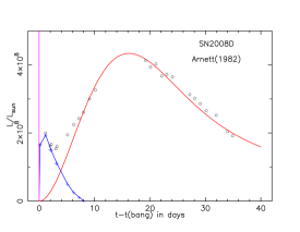
Figure 7: Bolometric light curves for SN2008D (circles) compared to analytic models fitted to the luminosity peak at 20 days (red line). V-magnitudes from this Ib supernova (Bianco, et al., 2014) are bolometrically corrected using Fig. 9 of Modjaz, et al. (2008), and are shown as circles. The X-ray spike found by Soderberg et al. (2008) is shown (purple) at the origin in time and allows an accurate determination of explosion time. The difference between this purely radioactive part (red line) and the observations (circles) allow us to estimate the excess due to additional processes (blue line and pluses).

In order to compare bolometric light curve shapes to observational data, we correct the V-band magnitudes (Bianco, et al., 2014) using graphical extraction of the bolometric corrections from Fig. 9 in Modjaz, et al. (2008). From 1 to 30 days after outburst, the variation is not large.

In Fig. 7 an estimate of the bolometric light curve for SN 2008D is presented. There are three different pieces: (a) an X-ray burst (purple) at explosion time, (b) newly-found, underlying intermediate peak at about 2 days (blue), and (c) a large peak at about 16-20 days (red). We proceed to analyze each piece.

7.0.1 Main diffusive stage

The major diffusive part (c) is represented by an analytic light curve (red) with the parameters given in Table 4, and with $\kappa_{t}=0.09$ as used previously for SN2011fe and KSN2008b. For simplicity no attempt was made to correct for effects of varying leakage (opacity). In this approximation the evolution begins after the shock reaches the surface; there is no shock break-out included.

7.0.2 Break-out stage

The break-out (a) gives a spike in X-rays (Soderberg et al., 2008), followed by cooling of this near-surface region by radiative diffusion and by expansion, quickly merging to the lowest-order diffusion solution Arnett (1980, 1982); Pinto & Eastman (2000a). The break-out spike in luminosity (purple) is much brighter than the V-band luminosity, because of large bolometric error (the spike radiation begins as X-ray and cools to UV, and so is not UVOIR).

7.0.3 Intermediate peak

If we subtract the analytic model from the bolometric luminosity, there is an excess which coresponds to a peak located at $1<t\leq 8$ days. This is piece (b) referred to above and seen in Fig. 7 as blue. After this time the total luminosity is well represented by the analytic model (red), which is due only to radioactive decay. This intermediate peak (in blue) at $1<t<8$ days, following the initial X-ray spike, does not appear in SNe Ia. This use of the analytic model allows us to probe the underlying physics in more detail.

What might cause this intermediate peak? The possibilities are intriguing but not unique. For example:

(1) Shock heating of a clump of matter which was ejected to a radius $r>10^{14}$ cm prior to core collapse, perhaps due to pulsations and eruptive mass loss (Arnett & Meakin, 2016), could be responsible.

(2) A ⁵⁶Ni plume of modest mass due to Rayleigh-Taylor instabilities (for example, a mass of $0.028M_{\odot}$ in the plume, with $0.012M_{\odot}$ of ⁵⁶Ni and $0.3$ bethe of kinetic energy can reproduce the excess luminosity in Fig. 7, with little effect on the main peak).

(3) Many other possibilities which may be imagined due to activity in the newly-collapsed core (see, e.g., §6.1).

(4) The breakout might be more complex than now imagined, and relax in a broader peak, not a $\delta$-function.

The first two are likely to give variations from event to event, as might the last two. New instruments such as LSST should clarify the extent of such fluctuations in the light curve of SN Ibc at early times ($t<8$ days). In this paper we have attempted precise comparisons with a few selected data sets of high quality; this has the disadvantage that it may not span the space of natural variation, which may be large for SNe Ibc (Wheeler, Johnson & Clocchiatti, 2015).

Table 4 gives a moderately different set of parameters from Table 5 because: (1) the bang time was measured, (2) the shape of the light curve was fit, including the excess (intermediate peak), and (3) the leakage opacity was assumed the same as in SN2011fe (§3). For consistency a small correction for the shift in bang time due to variable leakage (opacity) should be made; for simplicity it was not.

The net result of fitting the inferred diffusion peak (blue) separately seems to be a smaller estimate of ejected mass and explosion energy for this SN Ib (compare Table 5 to Table 4), but these differences are not drastic. If the total mass at core collapse is $\sim 3.5M_{\odot}$, as we infer from Fig. 7, SN2008D could be the stripped core of a star of initially $12$—$15\,M_{\odot}$, for example.

Table 5: Parameters for model (red curve) of SN2008D (Fig. 7)

Variable	Symbol	Value
Mass ejecteda	$M_{ej}$	$2.0\,M_{\odot}$
Initial 56Ni	$M_{Ni}(0)$	$0.082\,M_{\odot}$
Initial radius	$R(0)$	$1.0\times 10^{10}$ cm
Velocity scale	$v_{sc}$	$1.38\times 10^{9}$ cm s-1
Opacity	$\kappa_{t}$	$0.09$ cm2 g-1
Explosion energy	$E_{sn}$	$2.3\times 10^{51}$ ergs

8 Conclusion

We have applied the Arnett (1982) model to a wide variety of high-quality data on type Iabc supernovae. In summary:

1. There is excellent agreement between the best SNIa bolometric data and analytic models (which are bolometric).

2. There is an important problem of uniqueness; multiple combinations of parameters may all explain a given light curve. Light curves should be used, but with care, as probes of the supernova engine for core collapse supernovae (SNIbc). A light curve fit might have little to do with details of core collapse.

3. The best very early SNIa data show a deviation from the analytic models, which is easily removed by the relaxation of the assumption of strictly constant leakage time (opacity) at these times. This also slightly affects the inferred time from explosion to peak light.

4. Kepler data for KSN2011b may already indicate the presence of turbulent mixing during the explosion. It provides observational support for a slowly varying leakage time (mean opacity).

5. Arnett’s model may be generalized to SNIbc; for SN 2008D, inclusion of radioactive plumes or pre-collapse eruptions are among the possible causes of excess radiation.

6. Arnett’s rule deals with the radioactive heating of the plasma, and so includes effects of gamma-ray escape.

7. The SNe Ib, 2008D, is consistent with the explosion of a stripped-envelope star of initially 12–15$M_{\odot}$, possibly with a small radioactive plume.

Appendix A Nuclear Data

The data for the nuclear decay of ⁵⁶Ni and ⁵⁶Co in the analytic light curves is documented in Table 6.

Table 6: Nuclear physics data^a

Variable	Symbol	Nucleus	Value
Half-life	$\tau_{1\over 2}$	56Ni	$6.075$ days
		56Co	$77.236$ days
Total gamma energy	Eγ	56Ni	1.750 MeV
		56Co	3.610 MeV
Positron KE	E${}_{\beta^{+}}$	56Co	0.120 MeV
Energy release rates	$\epsilon_{Ni}$	56Ni	$3.9805\times 10^{10}$ erg/g/s
	$\epsilon_{Co}(\gamma)$	56Co	$6.4552\times 10^{9}$ erg/g/s
	$\epsilon_{Co}(\beta^{+})^{b}$	56Co	$2.1458\times 10^{8}$ erg/g/s

Appendix B Light curve equations

A more versatile method for solution of the Arnett (1982) model is to use four coupled ordinary differential equations, which we document below.

B.1 Equations for Arnett (1982) model

1. The first law of thermodynamics,

   $$dE/dt+PdV/dt=\epsilon_{deposit}-\partial L/\partial m$$

   becomes, upon integrating over the co-moving spatial variables (Arnett, 1982) and assuming dominant radiation pressure,

   $$d\phi(t)/dt=R(t)/R(0)$$

   $$\Big{(}M_{Ni}\Big{[}(\epsilon_{Ni}X_{Ni}+\epsilon_{Co}X_{Co})D$$

   $$+\epsilon_{Co}^{+}X_{Co}\Big{]}-\phi(t)/\tau_{dif}\Big{)},$$

   where $D$ is the deposition function of Colgate, Petschek & Kriese (1980) for $\gamma$-rays, and $\tau_{dif}=\kappa_{t}M_{ej}/(13.7cR(0))$, and $\phi(t)=a[(T(t)R(t))/T(0)R(0)]^{4}$. This is mathematically equivalent to Eq. 1 of Katz, Kushnir & Dong (2013).

2. Constant homologous expansion (Hubble flow):

   $$dR/dt=v_{sc},$$

   where $v_{sc}=\Big{(}10E_{KE}/3M_{ej}\Big{)}^{1\over 2},$

3. ⁵⁶N decay:

   $$dX_{Ni}/dt=-X_{Ni}/\tau_{Ni},$$

4. ⁵⁶Co decay:

   $$dX_{Co}/dt=-dX_{Ni}/dt-X_{Co}/\tau_{Co},$$

See also Table 6.

These equations are integrated by Runge-Kutta methods to a global accuracy of better than one part in $10^{8}$. For the same physical assumptions concerning escape of $\gamma$-rays, i.e., the function $D$, these equations and the integral approach of Katz, Kushnir & Dong (2013) should give consistent results (fitting the light curve with this approach may give more information, as seen in §7).

B.2 Changes and extensions

To include another radioactivity, add a new decay equation (like 3 annd 4), and add the new plasma heating to 1.

To add a new source of energy (magnetar, accretion disk, etc.), define a plasma heating rate as a function of time and add to 1.

To do energy tests or a Katz, Kushnir & Dong (2013) analysis, add new equations and variables (integrands) to integrate the energy types over time.

Typos do happen, but try to validate and verify before publishing (e.g., reproduce Figure 1 for the same parameters).

References

- Abarzhi (2010) Abarzhi, S. I., 2010, Phil. Trans. R. Soc. A, 368, 1809
- Abarzhi & Rosner (2010) Abarzhi, S. I., & Rosner, R., 2010, Physica Scripta, T142, 014012
- Arnett (1971) Arnett, W. D., 1971, ApJ, 163, 11
- Arnett & Falk (1976) Arnett, W. D. & Falk, S. W., 1976, ApJ, 210, 733
- Arnett (1977) Arnett, W. D., 1977, 8th Texas Symposium on Relativistic Astrophysics, 302, Ann. N. Y. Acad. Sci., 90
- Arnett (1979) Arnett, W. D., 1979, ApJ, 230, L37
- Arnett (1980) Arnett, W. D., 1980, ApJ, 237, 541
- Arnett (1982) Arnett, W. D., 1982, ApJ, 253, 785
- Arnett (1988) Arnett, W. D., 1988, ApJ, 331, 377
- Arnett (1996) Arnett, D., 1996, Supernovae and Nucleosynthesis, Princeton University Press, Princeton NJ
- Arnett & Meakin (2011) Arnett, W. D. & Meakin, C., 2011, ApJ, 733, 78
- Arnett & Meakin (2016) Arnett, W D., & Meakin, C., 2016, Reports of Prog. Phys.
- Arnett, et al. (2015) Arnett, W. D., Meakin, C. A., Viallet, M., Campbell, S. W., Lattanzio, J. C. & Mocák, M., 2015, ApJ, 809, 30
- Bayless, et al. (2013) Bayless, A. J., Even, W., Frey, L. H., Fryer, C. L., Roming, P. W. A., Young, P. A. 2015, ApJ, 805, 98
- Bianco, et al. (2014) Bianco, F. B., Modjaz, M., Hicken, M., Friedman, A., Kirshner, R. P., Bloom, J. S., Challis, P., Marion, G. H., Wood-Vasey, W. M., & Rest, A., 2014, ApJS, 213, 19
- Blondin, et al. (2013) Blondin, S., Dessart, L., Hillier, D. J., Khokhlov, A. M., 2013, MNRAS, 429, 2127
- Chevalier (1976) Chevalier, R. A., 1976, ApJ, 208, 826
- Chevalier & Kirshner (1978) Chevalier, R. A. & Kirshner, R. P., 1978, ApJ, 219, 931
- Chevalier & Fransson (2008) Chevalier, R. A. & Fransson, C. 2008, ApJ, 683, L135
- Clayton (1968) Clayton, D. D., 1968, Principles of Stellar Evolution and Nucleosynthesis, McGraw-Hill, New York
- Colgate & McKee (1969) Colgate, S. A., 1969, ApJ, 157, 623
- Colgate, Petschek & Kriese (1980) Colgate, S. A., Petschek, A. G., & Kriese, J. T., 1980, ApJ, 237, L133
- Dessart, et al. (2014) Dessart, L., Hillier, D. J., Blondin, S., Khokhlov, A., 2014, MNRAS, 441, 3249
- Dessart, et al. (2015) Dessart, L., Hillier, D. J., Woosley, S. E., Livne, E., Waldman, R., Yoon, S-C., Langer, N., 2015, MNRAS, 453, 2189
- Dessart, et al. (2016) Dessart, L., Hillier, D. J., Woosley, S. E., Livne, E., Waldman, R., Yoon, S-C., Langer, N., 2016, MNRAS, 458, 1618
- Falk (1978) Falk, S. W., 1978, ApJ, 226, L133
- Falk & Arnett (1973) Falk, S. W., & Arnett, W. D., 1973, ApJ, 180, L65
- Falk & Arnett (1977) Falk, Sydney W. & Arnett, W. David, 1977, ApJS, 33, 515
- Fesen & Milisavljevic (2016) Fesen, R. A., & Milisavljevic, D., 2016, ApJ, 818, 17
- Firth, et al. (2015) Firth, F. E., Sullivan, M., Gal-Yam, A., Howell, D. A., Maguire, K., Nugent, P., Piro, A. L., Baltay, C., Feindt, U., Hadjiyksta, E., McKinnon, R., Ofek, E., Rabinoowitz, D., Walker, E. S., 2015, MNRAS, 446, 3895
- Fryxell, Arnett & Müller (1991) Fryxell, B. A., Arnett, W. D., & Müller, E., 1991, ApJ, 367, 619
- Gonzalez-Gaitán, et al. (2012) Gonzalez-Gaitán, S., Conley, A., Bianco, F. B., et al., 2012, ApJ, 745, 44
- Hamuy, et al. (2003) Hamuy, M., Phillips, M., Suntzeff, N., Maza, J., 2003, IAUC, 8151
- Hoeflich, Khoklov & Mueller (1991) Hoeflich, P., Khoklov, A., & Müller, E., 1991, A&A, 248, L7
- Katz, Kushnir & Dong (2013) Katz, B., Kushnir, D., & Dond, S., 2013, arXiv:1301..6766v1.
- Kirshner & Chevalier (1977) Kirshner, R. P. & Chevalier, R. A., 1977, ApJ, 218, 142
- Landau & Lifshitz (1959) Landau, L. D. & Lifshitz, E. M., 1959, Fluid Mechanics, Pergamon Press, London.
- Landau & Lifshitz (1969) Landau, L. D. & Lifshitz, E. M., 1969, Statistical Physics, 2nd Ed., Addison–Wesley, Reading MA.
- Lantz et al. (2004) Lantz, B., Aldering, G., Antilogus, P., et al. 2004, Proc. SPIE, 5249, 146
- Magee et al. (1995) Magee, N. H., Abdallah, J., Jr., Clark, R. E. H., Cohen, J. S., Collins, L. A., Csanak, G., Fontes, C. J., Gauger, A., Keady, J. J., Kilcrease, Merts, A. L. 1995, in ASP Conf. Ser. 78, Astrophysical Applications of Powerful New Databases, ed. S. J. Adelman & W. L. Wiese (ASan Francisco, CA: ASP). 51 Landau, L. D. & Lifshitz, E. M., 1969, Statistical Physics, 2nd Ed., Addison–Wesley, Reading MA.
- Modjaz, et al. (2008) Modjaz, M., Li, W., Butler, N., et al., 2009, ApJ, 702, 226
- Müller, Fryxell, B. & Arnett, D. (1991) Müller, E., Fryxell, B. & Arnett, D., 1991, A&A, 251, 505
- Munari, et al. (2013) Munari, U., et al., 2013, New Astronomy, 20, 30
- Nadyozhin (1994) Nadyozhin, D. K., 1994, ApJS, 92, 527
- Nugent, et al. (2011) Nugent, P. E., Sullivan, M., Cenko, S. B., et al., 2011, Nature, 480, 344
- Olling, et al. (2015) Olling, R., Mushotzky, R., Shaya, E., Rest, A., Garnavich, P., Tucker, B., Kasen, D., Margheim, S., & Filippenko, A., 2015, Nature, 521, 332
- Pereira, et al. (2013) Pereira, R., Thomas, R. C., Aldering, G., et al., 2013, A&A, 554, A27
- Phillips (1993) Phillips, M., 1993, BAAS, 182, 2907
- Pinto & Eastman (2000a) Pinto, P. A., & Eastman, R., 2000a, ApJ, 530, 744
- Pinto & Eastman (2000b) Pinto, P. A., & Eastman, R., 2000b, ApJ, 530, 757
- Pinto & Eastman (2000c) Pinto, P. A., & Eastman, R., 2000c, New Astronomy, 6, 307
- Pope (2000) Pope, S. B., 2000, Turbulent Flows, Cambridge University Press, Cambridge, GB
- Piro & Nakar (2013) Piro, A. L., & Nakar, E., 2013, ApJ, 769, 67
- Riess, et al. (1999) Riess, A., 1999, AJ, 118, 2675
- Röpke, et al. (2012) Röpke, F. K., Kromer. M., Seitenzahl, I. R., et al., 2012, ApJ, 750:L19
- Seitenzahl, Taubenberger & Sim (2009) Seitenzahl, I. R., Taubenberger, S., & Sim, S. A.. 2009, MNRAS, 400, 531
- Smith (2017) Smith, Nathan, arXiv:1612.02006, to be published in the Supernova Handbook
- Smitka, et al. (2016) Smitka, M., et al., in preparation
- Soderberg et al. (2008) Soderberg, A. M., Berger, E., Page, K. L, et al. 2008, Nature, 453, 469
- Swisher, et al. (2015) Swisher, N. C., Kuranz, C. C., Arnett, D., Hurricane, O., Remington, B. A., Robey, H. F., & Abarshi, S. I., 2015, Physics of Plasmas, 22, 102707
- Tartaglia, et al., (2016) Tartaglia, L., Fraser, M., Sand, D. J., Valenti, S., Smartt, S. J., McCully,, C., et al., 2016, arXiv: 1611.00419v1
- Truran, Arnett & Cameron (1967) Truran, J. W., Arnett, W. D., & Cameron, A. G. W., 1967, Can. J. Phys., 45, 231
- Valenti, et al. (2008) Valenti, S., Benetti, S., Cappellaro, E., Patat, F., Mazzali, P., Turatto, M., Hurley, K., Maeda, K., Gal-Yam, A., Foley, R. J., Filippenko, A. V., Pastorello, A., Challis, P., Frontera, F., Harutyunyan, A., Iye, M., Kawabata, K., Kirshner, R. P., Li, W., Lipkin, Y. M., Matheson, T., Nomoto, K., Ofek, E. O., Ohyama, Y., Pian, E., Poznanski, D., Salvo, M., Sauer, D. N., Schmidt, B. P., Soderberg, A., & Zampieri, L., 2008, MNRAS, 383, 1485
- Waxman et al. (2007) Waxman, E., M?esza?ros, P., & Campana, S. 2007, ApJ, 667, 351
- Wheeler, Johnson & Clocchiatti (2015) Wheeler, J. C., Johnson, V., & Clocchiattii, A., 2015, MNRAS, 450, 1295
- Woosley & Weaver (1986) Woosley, S. E. & Weaver, T. A., 1986, ARA&A, 24, 205
- Zheng, et al. (2013) Zheng, W., et al., ApJ, 778, L15
- Zingale, et al. (2011) Zingale, M., Nonaka, A., Almgren, A. S., Bell, J. B., Malone, C. M., & Woosley, S. E., 2011, ApJ, 740, 8