Some Relations for Quark Confinement and Chiral Symmetry Breaking in QCD

Abstract

We analytically study the relation between quark confinement and spontaneous chiral-symmetry breaking in QCD. In terms of the Dirac eigenmodes, we derive some formulae for the Polyakov loop, its fluctuations, and the string tension from the Wilson loop. We also investigate the Polyakov loop in terms of the eigenmodes of the Wilson, the clover and the domain wall fermion kernels, respectively. For the confinement quantities, the low-lying Dirac/fermion eigenmodes are found to give negligible contribution, while they are essential for chiral symmetry breaking. These relations indicate no direct one-to-one correspondence between confinement and chiral symmetry breaking in QCD, which seems to be natural because confinement is realized independently of the quark mass.

1 Introduction

Color confinement and spontaneous chiral-symmetry breaking NJL61 are two outstanding nonperturbative phenomena in QCD, and they and their relation DSI14 ; DRSS15 ; SDI16 have been studied as one of the important difficult problems in theoretical particle physics. For quark confinement, the Polyakov loop $\langle L_{P}\rangle$ is one of the typical order parameters, which relates to the single-quark free energy $E_{q}$ as $\langle L_{P}\rangle\propto e^{-E_{q}/T}$ at temperature $T$. For chiral symmetry breaking, the standard order parameter is the chiral condensate $\langle\bar{q}q\rangle$, and low-lying Dirac modes are known to play the essential role BC80 .

A strong correlation between confinement and chiral symmetry breaking has been suggested by approximate coincidence between deconfinement and chiral-restoration temperatures R12 . Their correlation has been also suggested in terms of QCD-monopoles SST95 ; M95W95 , which topologically appear in QCD in the maximally Abelian (MA) gauge. By removing the monopoles from the QCD vacuum, confinement and chiral symmetry breaking are simultaneously lost in lattice QCD SST95 ; M95W95 . (See Fig. 1.) This indicates an important role of QCD-monopoles to both confinement and chiral symmetry breaking, and thus these two phenomena seem to be related via the monopole. However, the direct relation of confinement and chiral symmetry breaking is still unclear.

Actually, an accurate lattice QCD study AFKS06 shows about 25MeV difference between the deconfinement and the chiral-restoration temperatures, i.e., $T_{\rm deconf}\simeq 176{\rm MeV}$ and $T_{\rm chiral}\simeq 151{\rm MeV}$. We also note that some QCD-like theories exhibit a large difference between confinement and chiral symmetry breaking. For example, in an SU(3) gauge theory with adjoint-color fermions, the chiral transition occurs at much higher temperature, $T_{\rm chiral}\simeq 8T_{\rm deconf}$ KL99 . In 1+1 QCD with $N_{f}\geq 2$, confinement is realized, but spontaneous chiral symmetry breaking does not occur, because of the Coleman-Mermin-Wagner theorem. Also in $N=1$ SUSY 1+3 QCD with $N_{f}=N_{c}+1$, while confinement is realized, chiral symmetry breaking does not occur. A recent lattice study of SU(2)-color QCD with $N_{f}=2$ shows that a confined but chiral-restored phase is realized at a large baryon density BIKMN16 .

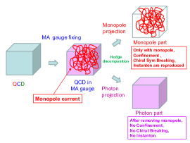
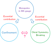
Figure 1: In the MA gauge, monopoles topologically appear. By removing the monopole from the QCD vacuum, confinement and chiral symmetry breaking are simultaneously lost SST95 ; M95W95 . This means crucial role of monopoles to both confinement and chiral symmetry breaking, but does not mean the direct correspondence between them.

In this paper, considering the essential role of low-lying Dirac modes to chiral symmetry breaking R12 , we derive analytical relations between the Dirac modes and the confinement quantities, e.g., the Polyakov loop DSI14 , its fluctuations DRSS15 and the string tension SDI16 , in the lattice QCD formalism.

2 Dirac operator, Dirac eigenvalues and Dirac modes in lattice QCD

In this paper, we take an ordinary square lattice with spacing $a$ and the size $V\equiv N_{s}^{3}\times N_{t}$, and impose the standard temporal periodicity/anti-periodicity for gluons/quarks. In lattice QCD, the gauge variable is expressed as the link-variable $U_{\mu}(s)\equiv{\rm e}^{iagA_{\mu}(s)}$ with the gauge coupling $g$ and the gluon field $A_{\mu}(x)$, and the simple Dirac operator and the covariant derivative operator are given as

$$\not\!\!\hat{D}=\frac{1}{2a}\sum_{\mu=1}^{4}\gamma_{\mu}(\hat{U}_{\mu}-\hat{U}_{-\mu}),\quad\hat{D}_{\mu}=\frac{1}{2a}(\hat{U}_{\mu}-\hat{U}_{-\mu}),$$ (1)

where the link-variable operator $\hat{U}_{\pm\mu}$ DSI14 ; DRSS15 ; SDI16 ; GIS12 is defined by

$$\langle s|\hat{U}_{\pm\mu}|s^{\prime}\rangle=U_{\pm\mu}(s)\delta_{s\pm\hat{\mu},s^{\prime}},$$ (2)

with $U_{-\mu}(s)\equiv U^{\dagger}_{\mu}(s-\hat{\mu})$. This simple Dirac operator $\hat{\not\!\!D}$ is anti-hermite and satisfies

$$\hat{\not\!\!D}_{s^{\prime},s}^{\dagger}=-\hat{\not\!\!D}_{s,s^{\prime}}.$$ (3)

We define the normalized Dirac eigenmode $|n\rangle$ and the Dirac eigenvalue $\lambda_{n}$,

$$\hat{\not\!\!D}|n\rangle=i\lambda_{n}|n\rangle\quad(\lambda_{n}\in{\bf R}),\qquad\langle m|n\rangle=\delta_{mn}.$$ (4)

Because of anti-hermiticity of $\hat{\not\!\!D}$, the Dirac eigenmode $|n\rangle$ satisfies the complete-set relation,

$$\sum_{n}|n\rangle\langle n|=1.$$ (5)

In lattice QCD, any functional trace becomes a sum over all the space-time site, i.e., ${\rm Tr}=\sum_{s}{\rm tr}$, which is defined for each lattice gauge configuration. For enough large volume lattice, e.g., $N_{s}\rightarrow\infty$, the functional trace is proportional to the gauge ensemble average, ${\rm Tr}\leavevmode\nobreak\ \hat{O}=\sum_{s}{\rm tr}\leavevmode\nobreak\ \hat{O}\propto\langle\hat{O}\rangle_{\rm gauge\leavevmode\nobreak\ ave.}$, for any operator $\hat{O}$. Note also that, because of the definition of $\hat{U}_{\pm\mu}$ in Eq.(2), the functional trace ${\rm Tr}(\hat{U}_{\mu_{1}}\hat{U}_{\mu_{2}}\cdots\hat{U}_{\mu_{N}})$ of any product of link-variable operators corresponding to “non-closed line” is exactly zero DSI14 ; DRSS15 ; SDI16 at each lattice gauge configuration, before taking the gauge ensemble average.

In this paper, we mainly use the lattice unit, $a=1$, for the simple notation.

3 Polyakov loop and Dirac modes in temporally odd-number lattice QCD

To begin with, we study the Polyakov loop and Dirac modes in temporally odd-number lattice QCD DSI14 ; DRSS15 ; SDI16 , where the temporal lattice size $N_{t}(<N_{s})$ is odd. In general, only gauge-invariant quantities such as closed loops and the Polyakov loop survive in QCD, according to the Elitzur theorem R12 . All the non-closed lines are gauge-variant and their expectation values are zero.

Now, we consider the functional trace DSI14 ; DRSS15 ; SDI16 ,

$$I\equiv{\rm Tr}_{c,\gamma}(\hat{U}_{4}\hat{\not\!\!D}^{N_{t}-1})=\sum_{n}\langle n|\hat{U}_{4}\not\!\!\hat{D}^{N_{t}-1}|n\rangle=i^{N_{t}-1}\sum_{n}\lambda_{n}^{N_{t}-1}\langle n|\hat{U}_{4}|n\rangle,$$ (6)

where ${\rm Tr}_{c,\gamma}\equiv\sum_{s}{\rm tr}_{c}{\rm tr}_{\gamma}$ includes the sum over all the four-dimensional site $s$ and the traces over color and spinor indices. In Eq.(6), we have used the completeness of the Dirac mode, $\sum_{n}|n\rangle\langle n|=1$.

From Eq.(1), $\hat{U}_{4}\hat{\not\!\!D}^{N_{t}-1}$ is expressed as a sum of products of $N_{t}$ link-variable operators. Then, $\hat{U}_{4}\hat{\not\!\!D}^{N_{t}-1}$ includes many trajectories with the total length $N_{t}$, as shown in Fig. 2.

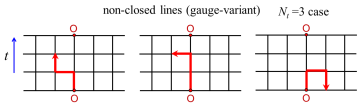
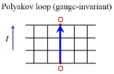
Figure 2: Partial examples of the trajectories in $I={\rm Tr}_{c,\gamma}(\hat{U}_{4}\hat{\not\!\!D}^{N_{t}-1})$. For each trajectory, the total length is $N_{t}$, and the “first step” is positive temporal direction, $\hat{U}_{4}$. All the trajectories with the odd length $N_{t}$ cannot form a closed loop on the square lattice, so that they are gauge-variant and give no contribution, except for the Polyakov loop.

Note that all the trajectories with the odd-number length $N_{t}$ cannot form a closed loop on the square lattice, and give gauge-variant contribution, except for the Polyakov loop. Thus, in $I={\rm Tr}_{c,\gamma}(\hat{U}_{4}\hat{\not\!\!D}^{N_{t}-1})$, only the Polyakov-loop can survive as the gauge-invariant component, and $I$ is proportional to the Polyakov loop $L_{P}$. Actually, we can mathematically derive the relation of

$$I={\rm Tr}_{c,\gamma}(\hat{U}_{4}\hat{\not\!\!D}^{N_{t}-1})={\rm Tr}_{c,\gamma}\{\hat{U}_{4}(\gamma_{4}\hat{D}_{4})^{N_{t}-1}\}=4{\rm Tr}_{c}(\hat{U}_{4}\hat{D}_{4}^{N_{t}-1})=\frac{4}{2^{N_{t}-1}}{\rm Tr}_{c}\{\hat{U}_{4}^{N_{t}}\}=-\frac{4N_{c}V}{2^{N_{t}-1}}L_{P},$$ (7)

where the last minus reflects the temporal anti-periodicity of $\hat{\not\!\!D}$ SDI16 . (Because of Eq.(2), the functional trace of “non-closed line” is exactly zero DSI14 ; DRSS15 ; SDI16 at each lattice gauge configuration.)

In this way, we obtain the analytical relation between the Polyakov loop $L_{P}$ and the Dirac modes in QCD on the temporally odd-number lattice DSI14 ; DRSS15 ; SDI16 ,

$$L_{P}=-\frac{(2i)^{N_{t}-1}}{4N_{c}V}\sum_{n}\lambda_{n}^{N_{t}-1}\langle n|\hat{U}_{4}|n\rangle,\qquad\langle L_{P}\rangle=-\frac{(2i)^{N_{t}-1}}{4N_{c}V}\left\langle\sum_{n}\lambda_{n}^{N_{t}-1}\langle n|\hat{U}_{4}|n\rangle\right\rangle_{\rm gauge\leavevmode\nobreak\ ave.},$$ (8)

which are mathematically robust. From Eq.(8), one can investigate each Dirac-mode contribution to the Polyakov loop. As a remarkable fact, low-lying Dirac modes give negligible contribution to the Polyakov loop, because of the suppression factor $\lambda_{n}^{N_{t}-1}$ in Eq.(8) DSI14 ; DRSS15 ; SDI16 . In lattice QCD calculations, we have numerically confirmed the relation (8) and tiny contribution of low-lying Dirac modes to the Polyakov loop in both confined and deconfined phases DSI14 .

4 Polyakov-loop fluctuations and Dirac eigenmodes

Next, we investigate Polyakov-loop fluctuations. As shown in Fig. 3(a), the Polyakov loop $L_{P}$ has fluctuations in longitudinal and transverse directions. We define its longitudinal and transverse components, $L_{L}\equiv{\rm Re}\leavevmode\nobreak\ \tilde{L}_{P}$ and $L_{T}\equiv{\rm Im}\leavevmode\nobreak\ \tilde{L}_{P}$, with $\tilde{L}_{P}\equiv L_{P}\leavevmode\nobreak\ e^{2\pi ik/3}$ where $k\in\{0,\pm 1\}$ is chosen such that the $Z_{3}$-transformed Polyakov loop lies in its real sector DRSS15 ; LFKRS13 . We introduce the Polyakov-loop fluctuations as $\chi_{A}\propto\langle|L_{P}|^{2}\rangle-|\langle L_{P}\rangle|^{2}$, $\chi_{L}\propto\langle L_{L}^{2}\rangle-\langle L_{L}\rangle^{2}$ and $\chi_{T}\propto\langle L_{T}^{2}\rangle-\langle L_{T}\rangle^{2}$. Some ratios of them largely change around the transition temperature, and can be good indicators of the QCD transition LFKRS13 .

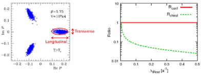
Figure 3: (a) The scatter plot of the Polyakov loop in lattice QCD. (b) The lattice QCD result for the infrared Dirac-mode cut quantities of $R_{\rm conf}(\Lambda_{\rm IRcut})\equiv R_{A}(\Lambda_{\rm IRcut})/R_{A}$ and $R_{\rm chiral}(\Lambda_{\rm IRcut})\equiv\langle\bar{q}q\rangle_{\Lambda_{\rm IRcut}}/\langle\bar{q}q\rangle$ plotted against the infrared cutoff $\Lambda_{\rm IRcut}$ introduced on Dirac eigenvalues DRSS15 . This figure is taken from Ref.DRSS15 . In contrast to the sensitivity of the chiral condensate $R_{\rm chiral}$, the Polyakov-loop fluctuation ratio $R_{\rm conf}$ is almost unchanged against the infrared cutoff $\Lambda_{\rm IRcut}$ of the Dirac mode.

In temporally odd-number lattice QCD, we derive Dirac-mode expansion formulae for Polyakov-loop fluctuations DRSS15 . For example, the Dirac spectral representation of the ratio $R_{A}\equiv\chi_{A}/\chi_{L}$ is

$$R_{A}=\frac{\left\langle\left|\sum_{n}\lambda_{n}^{N_{t}-1}\langle n|\hat{U}_{4}|n\rangle\right|^{2}\right\rangle_{\rm gauge\leavevmode\nobreak\ ave.}-\left\langle\left|\sum_{n}\lambda_{n}^{N_{t}-1}\langle n|\hat{U}_{4}|n\rangle\right|\right\rangle^{2}_{\rm gauge\leavevmode\nobreak\ ave.}}{\left\langle\left(\sum_{n}\lambda_{n}^{N_{t}-1}{\rm Re}\left(\mathrm{e}^{2\pi ik/3}\langle n|\hat{U}_{4}|n\rangle\right)\right)^{2}\right\rangle_{\rm gauge\leavevmode\nobreak\ ave.}-\left\langle\sum_{n}\lambda_{n}^{N_{t}-1}{\rm Re}\left(\mathrm{e}^{2\pi ik/3}\langle n|\hat{U}_{4}|n\rangle\right)\right\rangle^{2}_{\rm gauge\leavevmode\nobreak\ ave.}}.$$ (9)

Because of the reduction factor $\lambda_{n}^{N_{t}-1}$ in the Dirac-mode sum, all the Polyakov-loop fluctuations are almost unchanged by removing low-lying Dirac modes DRSS15 .

As the demonstration, we show in Fig. 3(b) the lattice QCD result of $R_{\rm conf}(\Lambda_{\rm IRcut})\equiv R_{A}(\Lambda_{\rm IRcut})/R_{A}$ and $R_{\rm chiral}(\Lambda_{\rm IRcut})\equiv\langle\bar{q}q\rangle_{\Lambda_{\rm IRcut}}/\langle\bar{q}q\rangle$ in the presence of the infrared Dirac-mode cutoff $\Lambda_{\rm IRcut}$ introduced on Dirac eigenvalues DRSS15 . As the Dirac-mode cutoff $\Lambda_{\rm IRcut}$ increases, the chiral condensate $R_{\rm chiral}$ rapidly reduces, but the Polyakov-loop fluctuation ratio $R_{\rm conf}$ is almost unchanged DRSS15 .

5 The Wilson loop and Dirac modes on arbitrary square lattices

In this section, we investigate the Wilson loop and the string tension in terms of the Dirac modes, on arbitrary square lattices with any number of $N_{t}$ SDI16 . We consider the ordinary Wilson loop of the $R\times T$ rectangle. The Wilson loop on the $x_{i}$-$t$ ($i=1,2,3$) plane is expressed by the functional trace,

$$W\equiv{\rm Tr}_{c}\hat{U}_{i}^{R}\hat{U}_{-4}^{T}\hat{U}_{-i}^{R}\hat{U}_{4}^{T}={\rm Tr}_{c}\hat{U}_{\rm staple}\hat{U}_{4}^{T},$$ (10)

where we introduce the “staple operator” $\hat{U}_{\rm staple}$ defined by

$$\hat{U}_{\rm staple}\equiv\hat{U}_{i}^{R}\hat{U}_{-4}^{T}\hat{U}_{-i}^{R}.$$ (11)

In fact, the Wilson-loop operator is factorized as a product of $\hat{U}_{\rm staple}$ and $\hat{U}_{4}^{T}$, as shown in Fig. 4.

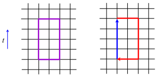
Figure 4: Left: The Wilson loop $W$ on a $R\times T$ rectangle. Right: The factorization of the Wilson-loop operator as a product of $\hat{U}_{\rm staple}\equiv\hat{U}_{i}^{R}\hat{U}_{-4}^{T}\hat{U}_{-i}^{R}$ and $\hat{U}_{4}^{T}$ SDI16 . Here, $T$, $R$ and the lattice size $N_{s}^{3}\times N_{t}$ are arbitrary.

5.1 Case of even T

In the case of even number $T$, we consider the functional trace,

$$J\equiv{\rm Tr}_{c,\gamma}\hat{U}_{\rm staple}\hat{\not\!\!D}^{T}=\sum_{n}\langle n|\hat{U}_{\rm staple}{\not\!\!D}^{T}|n\rangle=(-)^{\frac{T}{2}}\sum_{n}\lambda_{n}^{T}\langle n|\hat{U}_{\rm staple}|n\rangle,$$ (12)

where the completeness of the Dirac mode, $\sum_{n}|n\rangle\langle n|=1$, is used. Similarly in Sec. 3, one finds

$$J=\frac{1}{2^{T}}{\rm Tr}_{c,\gamma}\hat{U}_{\rm staple}\left[\sum_{\mu=1}^{4}\gamma_{\mu}(\hat{U}_{\mu}-\hat{U}_{-\mu})\right]^{T}\!\!\!=\frac{1}{2^{T}}{\rm Tr}_{c,\gamma}\hat{U}_{\rm staple}(\gamma_{4}\hat{U}_{4})^{T}=\frac{4}{2^{T}}{\rm Tr}_{c}\hat{U}_{\rm staple}\hat{U}_{4}^{T}=\frac{4}{2^{T}}W,$$ (13)

at each lattice gauge configuration. In fact, $\hat{U}_{4}$ must be selected in all the $\hat{\not\!\!D}\propto\sum_{\mu}\gamma_{\mu}(\hat{U}_{\mu}-\hat{U}_{-\mu})$ in $\hat{\not\!\!D}^{T}$, to form a loop in the functional trace. All other terms correspond to non-closed lines and give exactly zero, because of the definition of $\hat{U}_{\pm\mu}$ in Eq.(2). Thus, we obtain SDI16

$$W=\frac{(-)^{\frac{T}{2}}2^{T}}{4}\sum_{n}\lambda_{n}^{T}\langle n|\hat{U}_{\rm staple}|n\rangle.$$ (14)

Then, the inter-quark potential $V(R)$ is written as

$$V(R)=-\lim_{T\to\infty}\frac{1}{T}{\rm ln}\langle W\rangle=-\lim_{T\to\infty}\frac{1}{T}{\rm ln}\left|\left\langle\sum_{n}(2\lambda_{n})^{T}\langle n|\hat{U}_{\rm staple}|n\rangle\right\rangle\right|,$$ (15)

and the string tension $\sigma$ is expressed as

$$\sigma=-\lim_{R,T\to\infty}\frac{1}{RT}{\rm ln}\langle W\rangle=-\lim_{R,T\to\infty}\frac{1}{RT}{\rm ln}\left|\left\langle\sum_{n}\lambda_{n}^{T}\langle n|\hat{U}_{\rm staple}|n\rangle\right\rangle\right|.$$ (16)

Owing to the reduction factor $\lambda_{n}^{T}$ in the sum, the string tension $\sigma$, i.e., the confining force, is to be unchanged by the removal of the low-lying Dirac-mode contribution.

5.2 Case of odd T

In the case of odd number $T$, the similar results can be obtained by considering

$$J\equiv{\rm Tr}_{c,\gamma}\hat{U}_{\rm staple}\hat{U}_{4}\hat{\not\!\!D}^{T-1}=\sum_{n}\langle n|\hat{U}_{\rm staple}\hat{U}_{4}{\not\!\!D}^{T-1}|n\rangle=(-)^{\frac{T-1}{2}}\sum_{n}\lambda_{n}^{T-1}\langle n|\hat{U}_{\rm staple}\hat{U}_{4}|n\rangle.$$ (17)

Actually, one finds

$$J=\frac{1}{2^{T-1}}{\rm Tr}_{c,\gamma}\hat{U}_{\rm staple}\hat{U}_{4}\left[\sum_{\mu=1}^{4}\gamma_{\mu}(\hat{U}_{\mu}-\hat{U}_{-\mu})\right]^{T-1}\!\!\!=\frac{1}{2^{T-1}}{\rm Tr}_{c,\gamma}\hat{U}_{\rm staple}\hat{U}_{4}(\gamma_{4}\hat{U}_{4})^{T-1}=\frac{4}{2^{T-1}}W,$$ (18)

and obtains for odd $T$ the similar formula of SDI16

$$W=\frac{(-)^{\frac{T-1}{2}}2^{T-1}}{4}\sum_{n}\lambda_{n}^{T-1}\langle n|\hat{U}_{\rm staple}\hat{U}_{4}|n\rangle.$$ (19)

Then, the inter-quark potential $V(R)$ and the sting tension $\sigma$ are written as

$$V(R) = -\lim_{T\to\infty}\frac{1}{T}{\rm ln}\langle W\rangle=-\lim_{T\to\infty}\frac{1}{T}{\rm ln}\left|\left\langle\sum_{n}(2\lambda_{n})^{T-1}\langle n|\hat{U}_{\rm staple}\hat{U}_{4}|n\rangle\right\rangle\right|,$$ (20)

$$\sigma = -\lim_{R,T\to\infty}\frac{1}{RT}{\rm ln}\langle W\rangle=-\lim_{R,T\to\infty}\frac{1}{RT}{\rm ln}\left|\left\langle\sum_{n}\lambda_{n}^{T-1}\langle n|\hat{U}_{\rm staple}\hat{U}_{4}|n\rangle\right\rangle\right|,$$ (21)

where $\sigma$ is unchanged by removing the low-lying Dirac-mode contribution due to $\lambda_{n}^{T-1}$ in the sum.

6 The Polyakov loop v.s. Wilson, clover and domain wall fermions

All the above formulae are mathematically correct, because we have just used the Elitzur theorem (or precisely Eq.(2) for $\hat{U}_{\pm\mu}$) and the completeness $\sum_{n}|n\rangle\langle n|=1$ on the Dirac operator (1). However, one may wonder the doublers R12 in the use of the simple lattice Dirac operator (1). In this section, we express the Polyakov loop with the eigenmodes of the kernel of the Wilson fermion R12 , the clover ($O(a)$-improved Wilson) fermion SW85 ; NNMS03 and the domain wall (DW) fermion K92 ; S93FS95 , respectively SDRS16 . In these fermionic kernel, light doublers are absent.

6.1 The Wilson fermion

The Wilson fermion kernel R12 can be described with the link-variable operator $\hat{U}_{\pm\mu}$ as SDRS16

$$\hat{K}=\hat{\not\!\!D}+m+\frac{r}{2a}\sum_{\mu=\pm 1}^{\pm 4}\gamma_{\mu}(\hat{U}_{\mu}-1)=\frac{1}{2a}\sum_{\mu=1}^{4}\gamma_{\mu}(\hat{U}_{\mu}-\hat{U}_{-\mu})+m+\frac{r}{2a}\sum_{\mu=1}^{4}\gamma_{\mu}(\hat{U}_{\mu}+\hat{U}_{-\mu}-2),$$ (22)

where each term of $\hat{K}$ includes one $\hat{U}_{\pm\mu}$ at most, and connects only the neighboring site or acts on the same site. Near the continuum, $a\simeq 0$, Eq.(22) becomes $\hat{K}\simeq(\hat{\not\!\!D}+m)+ar\hat{D}^{2}$ and the Wilson term $ar\hat{D}^{2}$ is $O(a)$.

For the Wilson fermion kernel $\hat{K}$, we define its eigenmode $|n\rangle\rangle$ and eigenvalue $\tilde{\lambda}_{n}$ as

$$\hat{K}|n\rangle\rangle=i\tilde{\lambda}_{n}|n\rangle\rangle,\quad\tilde{\lambda}_{n}\in{\bf C}.$$ (23)

Note that, without the Wilson term, the eigenmode of $\hat{K}=\hat{\not\!\!D}+m$ is the simple Dirac eigenmode $|n\rangle$, i.e., $\hat{K}|n\rangle=(i\lambda_{n}+m)|n\rangle$, and satisfies the completeness of $\sum_{n}|n\rangle\langle n|=1$. In the presence of the $O(a)$ Wilson term, $\hat{K}$ is neither hermite nor anti-hermite, and the completeness may include an $O(a)$ error,

$$\sum_{n}|n\rangle\rangle\langle\langle n|=1+O(a).$$ (24)

Now, on the lattice with $N_{t}=4l+1$, we consider the functional trace,

$$J\equiv{\rm Tr}(\hat{U}_{4}^{2l+1}\hat{K}^{2l}).$$ (25)

Using the quasi-completeness of Eq.(24) for the eigenmode $|n\rangle\rangle$, one finds, apart from an $O(a)$ error,

$$J\simeq\sum_{n}\langle\langle n|\hat{U}_{4}^{2l+1}{\hat{K}}^{2l}|n\rangle\rangle=\sum_{n}(i\tilde{\lambda}_{n})^{2l}\langle\langle n|\hat{U}_{4}^{2l+1}|n\rangle\rangle.$$ (26)

We note that the kernel $\hat{K}$ in Eq. (22) includes many terms, and $J\equiv{\rm Tr}(\hat{U}_{4}^{2l+1}\hat{K}^{2l})$ consists of products of link-variable operators, accompanying with $c$-number factors. In each product, the total number of $\hat{U}$ does not exceed $N_{t}$, because of Eq. (22). Each product gives a trajectory as shown in Fig. 5.

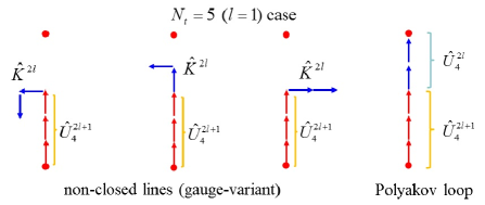
Figure 5: Some examples of the trajectories in $J\equiv{\rm Tr}(\hat{U}_{4}^{2l+1}\hat{K}^{2l})$ for the $N_{t}=5$ ($l=1$) case. The length does not exceed $N_{t}$ for each trajectory. Only the Polyakov loop $L_{P}$ can form a closed loop and survives in $J$.

Among the trajectories, however, only the Polyakov loop $L_{P}$ can form a closed loop and survives in $J$, so that one gets $J\propto L_{P}$. Thus, apart from an $O(a)$ error, we obtain SDRS16

$$L_{P}\propto\sum_{n}\tilde{\lambda}_{n}^{2l}\langle\langle n|\hat{U}_{4}^{2l+1}|n\rangle\rangle.$$ (27)

Due to the suppression factor of $\tilde{\lambda}_{n}^{2l}$ in the sum, one finds again small contribution from low-lying modes of $\hat{K}$ to the Polyakov loop $L_{P}$.

6.2 The clover (O(a)-improved Wilson) fermion

The clover fermion is an $O(a)$-improved Wilson fermion SW85 , and its kernel is expressed as SDRS16

$$\hat{K}=\frac{1}{2a}\sum_{\mu=1}^{4}\gamma_{\mu}(\hat{U}_{\mu}-\hat{U}_{-\mu})+m+\frac{r}{2a}\sum_{\mu=1}^{4}\gamma_{\mu}(\hat{U}_{\mu}+\hat{U}_{-\mu}-2)+\frac{arg}{2}\sigma_{\mu\nu}G_{\mu\nu},$$ (28)

with $\sigma_{\mu\nu}\equiv\frac{i}{2}[\gamma_{\mu},\gamma_{\nu}]$. Here, $G_{\mu\nu}$ is the clover-type lattice field strength defined by

$$G_{\mu\nu}\equiv\frac{1}{8}(P_{\mu\nu}+P^{\dagger}_{\mu\nu}),$$ (29)

with

$$P_{\mu\nu}(x)\equiv\langle x|(\hat{U}_{\mu}\hat{U}_{\nu}\hat{U}_{-\mu}\hat{U}_{-\nu}+\hat{U}_{\nu}\hat{U}_{-\mu}\hat{U}_{-\nu}\hat{U}_{\mu}+\hat{U}_{-\mu}\hat{U}_{-\nu}\hat{U}_{\mu}\hat{U}_{\nu}+\hat{U}_{-\nu}\hat{U}_{\mu}\hat{U}_{\nu}\hat{U}_{-\mu})|x\rangle.$$ (30)

The sum of the Wilson and the clover terms is $O(a^{2})$ near the continuum, and the clover fermion gives accurate lattice results NNMS03 . Since $G_{\mu\nu}$ acts on the same site, each term of $\hat{K}$ in Eq.(28) connects only the neighboring site or acts on the same site, so that one can use almost the same technique as the Wilson fermion case.

For the clover fermion kernel $\hat{K}$, we define its eigenmode $|n\rangle\rangle$ and eigenvalue $\tilde{\lambda}_{n}$ as

$$\hat{K}|n\rangle\rangle=i\tilde{\lambda}_{n}|n\rangle\rangle,\quad\tilde{\lambda}_{n}\in{\bf C},\quad\qquad\sum_{n}|n\rangle\rangle\langle\langle n|=1+O(a^{2}).$$ (31)

Again, on the lattice with $N_{t}=4l+1$, we consider the functional trace,

$$J\equiv{\rm Tr}(\hat{U}_{4}^{2l+1}\hat{K}^{2l})\simeq\sum_{n}\langle\langle n|\hat{U}_{4}^{2l+1}{\hat{K}}^{2l}|n\rangle\rangle=\sum_{n}(i\tilde{\lambda}_{n})^{2l}\langle\langle n|\hat{U}_{4}^{2l+1}|n\rangle\rangle,$$ (32)

where we have used the quasi-completeness for $|n\rangle\rangle$ in Eq.(31) within an $O(a^{2})$ error. $J\equiv{\rm Tr}(\hat{U}_{4}^{2l+1}\hat{K}^{2l})$ consists of products of link-variable operators, accompanying with $c$-number factors, and each product gives a trajectory as shown in Fig. 5. Among the trajectories, only the Polyakov loop $L_{P}$ can form a closed loop and survives in $J$, i.e., $J\propto L_{P}$. Thus, apart from an $O(a^{2})$ error, we obtain SDRS16

$$L_{P}\propto\sum_{n}\tilde{\lambda}_{n}^{2l}\langle\langle n|\hat{U}_{4}^{2l+1}|n\rangle\rangle,$$ (33)

and find small contribution from low-lying modes of $\hat{K}$ to the Polyakov loop $L_{P}$, due to $\tilde{\lambda}_{n}^{2l}$ in the sum.

6.3 The domain wall (DW) fermion

Finally, we consider the domain wall (DW) fermion K92 ; S93FS95 , where the “exact” chiral symmetry is realized in the lattice formalism by introducing an extra spatial coordinate $x_{5}$. The DW fermion is formulated in the five-dimensional space-time, and its (five-dimensional) kernel is expressed as

$$\hat{K}_{5}=\frac{1}{2a}\sum_{\mu=1}^{4}\gamma_{\mu}(\hat{U}_{\mu}-\hat{U}_{-\mu})+m+\frac{r}{2a}\sum_{\mu=1}^{4}\gamma_{\mu}(\hat{U}_{\mu}+\hat{U}_{-\mu}-2)+\gamma_{5}\hat{\partial}_{5}+M(x_{5}),$$ (34)

where the last two terms in the RHS are the kinetic and the mass terms in the fifth dimension. Here, $x_{5}$-dependent mass $M(x_{5})$ is introduced as shown in Fig.6, where $M_{0}=|M(x_{5})|=O(a^{-1})$ is taken to be large. As for the extra coordinate $x_{5}$, there are only kinetic and mass terms in $\hat{K}_{5}$, so that the eigenvalue problem is solved in the fifth direction, and chiral zero modes are found to appear K92 ; S93FS95 .

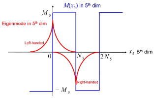
Figure 6: The construction of the domain wall (DW) fermion by introducing the fifth dimension of $x_{5}$ and the $x_{5}$-dependent mass $M(x_{5})$. There appear left- and right-handed chiral zero modes localized around $x_{5}=0$ and $x_{5}=N_{5}$, respectively.

For the five-dimensional DW fermion kernel $\hat{K}_{5}$, we define its eigenmode $|\nu\rangle$ and eigenvalue $\Lambda_{\nu}$ as

$$\hat{K}_{5}|\nu\rangle=i\Lambda_{\nu}|\nu\rangle,\quad\Lambda_{\nu}\in{\bf C},\quad\qquad\sum_{\nu}|\nu\rangle\langle\nu|=1+O(a).$$ (35)

Note that each term of $\hat{K}_{5}$ in Eq.(34) connects only the neighboring site or acts on the same site in the five-dimensional space-time, and hence one can use almost the same technique as the Wilson fermion case. On the lattice with $N_{t}=4l+1$, we consider the functional trace,

$$J\equiv{\rm Tr}(\hat{U}_{4}^{2l+1}\hat{K}_{5}^{2l})\simeq\sum_{\nu}\langle\nu|\hat{U}_{4}^{2l+1}{\hat{K}_{5}}^{2l}|\nu\rangle=\sum_{\nu}(i\Lambda_{\nu})^{2l}\langle\nu|\hat{U}_{4}^{2l+1}|\nu\rangle,$$ (36)

where the quasi-completeness for $|\nu\rangle$ in Eq.(35) is used. $J\equiv{\rm Tr}(\hat{U}_{4}^{2l+1}\hat{K}_{5}^{2l})$ consists of products of link-variable operators with other factors, and each product gives a trajectory as shown in Fig. 5 in the projected four-dimensional space-time. Among the trajectories, only the Polyakov loop $L_{P}$ can form a closed loop and survives in $J$, i.e., $J\propto L_{P}$. Thus, apart from an $O(a)$ error, we obtain

$$L_{P}\propto\sum_{\nu}\Lambda_{\nu}^{2l}\langle\nu|\hat{U}_{4}^{2l+1}|\nu\rangle.$$ (37)

Because of the simple $x_{5}$-dependence in $\hat{K}_{5}$ in Eq.(34), the extra degrees of freedom in the fifth dimension can be integrated out in the generating functional, and one obtains the four-dimensional physical-fermion kernel $\hat{K}_{4}$ S93FS95 . The physical fermion mode is given by the eigenmode $|n\rangle\rangle$ of $\hat{K}_{4}$,

$$\hat{K}_{4}|n\rangle\rangle=i\tilde{\lambda}_{n}|n\rangle\rangle,\quad\tilde{\lambda}_{n}\in{\bf C}.$$ (38)

We find that the four-dimensional physical fermion eigenvalue $\tilde{\lambda}_{n}$ of $\hat{K}_{4}$ can be approximated by the eigenvalue $\Lambda_{\nu}$ of the five-dimensional DW kernel $\hat{K}_{5}$ as

$$\Lambda_{\nu}=\tilde{\lambda}_{n_{\nu}}+O(M_{0}^{-2})=\tilde{\lambda}_{n_{\nu}}+O(a^{2}),$$ (39)

where $M_{0}=|M(x_{5})|=O(a^{-1})$ is taken to be large.

Combining with Eq.(37), apart from an $O(a)$ error, we obtain

$$L_{P}\propto\sum_{\nu}\tilde{\lambda}_{n_{\nu}}^{2l}\langle\langle\nu|\hat{U}_{4}^{2l+1}|\nu\rangle\rangle,$$ (40)

and find small contribution from low-lying physical-fermion modes of $\hat{K}_{4}$ to the Polyakov loop $L_{P}$, because of the suppression factor $\tilde{\lambda}_{n_{\nu}}^{2l}$ in the sum.

7 Summary and Concluding Remarks

In QCD, we have derived analytical relations between the Dirac modes and the confinement quantities such as the Polyakov loop, its fluctuations and the string tension in the lattice formalism, and have found negligible contribution from the low-lying Dirac modes to the confinement quantities.

We have also investigated the Polyakov loop in terms of the eigenmodes of the Wilson, the clover and the domain wall fermion kernels, respectively, and have obtained the similar results.

These relations indicate no direct one-to-one correspondence between confinement and chiral symmetry breaking. In other words, there is some independence of confinement from chiral properties in QCD. This seems natural because confinement is realized independently of the quark mass.

References

- (1) Y. Nambu and G. Jona-Lasinio, Phys. Rev 122, 345 (1961); Phys. Rev. 124, 246 (1961).
- (2) T. M. Doi, H. Suganuma and T. Iritani, Phys. Rev. D90, 094505 (2014).
- (3) T. M. Doi, K. Redlich, C. Sasaki and H. Suganuma, Phys. Rev. D92, 094004 (2015).
- (4) H. Suganuma, T. M. Doi and T. Iritani, Prog. Theor. Exp. Phys. 2016, 013B06 (2016).
- (5) T. Banks and A. Casher, Nucl. Phys. B169, 103 (1980).
- (6) H. -J. Rothe, “Lattice Gauge Theories”, 4th edition, (World Scientific, 2012), and its references.
- (7) H. Suganuma, S. Sasaki and H. Toki, Nucl. Phys. B435, 207 (1995).
- (8) O. Miyamura, Phys. Lett. B353, 91 (1995); R. M. Woloshyn, Phys. Rev. D51, 6411 (1995).
-
(9)
Y. Aoki, Z. Fodor, S.D. Katz and K.K. Szabo,
Phys. Lett. B643, 46 (2006);
Y. Aoki, G. Endrodi, Z. Fodor, S. D. Katz and K. K. Szabo, Nature 443, 675 (2006). - (10) F. Karsch and M. Lutgemeier, Nucl. Phys. B550 449, (1999).
- (11) V.V. Braguta, E.-M. Ilgenfritz, A.Yu. Kotov, A.V. Molochkov, A.A. Nikolaev, arXiv:1605.04090.
-
(12)
S. Gongyo, T. Iritani and H. Suganuma,
Phys. Rev. D86, 034510 (2012);
T. Iritani and H. Suganuma, Prog. Theor. Exp. Phys. 2014, 033B03 (2014). - (13) P. M. Lo, B. Friman, O. Kaczmarek, K. Redlich and C. Sasaki, Phys. Rev. D88, 014506 (2013); Phys. Rev. D88 074502 (2013).
- (14) B. Sheikholeslami and R. Wohlert, Nucl .Phys. B259, 572 (1985).
- (15) Y. Nemoto, N. Nakajima, H. Matsufuru and H. Suganuma, Phys. Rev. D68, 094505 (2003).
- (16) D. B. Kaplan, Phys. Lett. B288, 342 (1992).
- (17) Y. Shamir, Nucl. Phys. B406, 90 (1993); V. Furman and Y. Shamir, Nucl. Phys. B439, 54 (1995).
- (18) H. Suganuma, T. M. Doi, K. Redlich and C. Sasaki, arXiv:1610.02999 [hep-lat].