BliStrTune:
Hierarchical Invention of Theorem Proving Strategies

Abstract

Inventing targeted proof search strategies for specific problem sets is a difficult task. State-of-the-art automated theorem provers (ATPs) such as E allow a large number of user-specified proof search strategies described in a rich domain specific language. Several machine learning methods that invent strategies automatically for ATPs were proposed previously. One of them is the Blind Strategymaker (BliStr), a system for automated invention of ATP strategies.

In this paper we introduce BliStrTune – a hierarchical extension of BliStr. BliStrTune allows exploring much larger space of E strategies by interleaving search for high-level parameters with their fine-tuning. We use BliStrTune to invent new strategies based also on new clause weight functions targeted at problems from large ITP libraries. We show that the new strategies significantly improve E’s performance in solving problems from the Mizar Mathematical Library.

1 Introduction: ATP Strategy Invention

State-of-the-art automated theorem provers (ATPs) such as E Schulz [2002, 2013] and Vampire Kovács and Voronkov [2013] achieve their performance by using sophisticated proof search strategies and their combinations. Constructing good ATP search strategies is a hard task that is potentially very rewarding. Until recently, there has been, however, little research in this direction in the ATP community.

With the arrival of large ATP problem sets and benchmarks extracted from the libraries of today’s interactive theorem prover (ITP) systems Blanchette et al. [2016a, b]; Gauthier and Kaliszyk [2015]; Kaliszyk and Urban [2014, 2015], automated generation of targeted ATP strategies became an attractive topic. It seems unlikely that manual (“theory-driven”) construction of targeted strategies can scale to large numbers of ATP problems spanning many different areas of mathematics and computer science. Starting with Blind Strategymaker (BliStr) Urban [2015] that was used to invent E’s strategies for MaLARea Urban et al. [2008]; Kaliszyk et al. [2015b] on the 2012 Mizar@Turing competition problems Sutcliffe [2013], several systems have been recently developed to invent targeted ATP strategies Schäfer and Schulz [2015]; Kühlwein and Urban [2015]. The underlying methods used so far include genetic algorithms and iterated local search, as popularized by the ParamILS Hutter et al. [2009] system.

A particular problem of the methods based on iterated local search is that their performance degrades as the number of possible strategy parameters gets high. This is the case for E, where a domain specific language allows construction of astronomic numbers of strategies. This gets worse as more and more sophisticated templates for strategies are added to E, such as our recent family of conjecture-oriented weight functions implementing various notions of term-based similarity Jakubův and Urban [2016]. The pragmatic solution used in the original BliStr consisted of re-using manually pre-designed high-level strategy components, rather than allowing the system to explore the space of all possible strategies. This is obviously unsatisfactory.

In this work we introduce BliStrTune – a hierarchical extension of BliStr. BliStrTune allows exploring much larger space of E strategies by factoring the search into invention of good high-level strategy components and their low-level fine-tuning. The high-level and low-level inventions communicate to each other their best solutions, iteratively improving all parts of the strategy space. Together with our new conjecture-oriented weight functions, the hierarchical invention produces so far the strongest schedule of strategies on the small (bushy) versions of the Mizar@Turing problems. The improvement over Vampire 4.0 on the training set is nearly 10%, while the improvement on the testing (competition) set is over 5%.

The rest of the paper is organized as follows. Section 2 introduces the notion of proof search strategies, focusing on resolution/superposition ATPs and E prover. We also summarize our recent conjecture-oriented strategies that motivated the work on BliStrTune. Section 3 describes the ideas behind the original Blind Strategymaker based on the ParamILS system (see Section 3.1 for more details on ParamILS). Section 4 introduces the hierarchical invention algorithm and its implementation. The system is evaluated in several ways in Section 5, showing significant improvements over the original BliStr and producing significantly improved ATP strategies.

2 Proof Search Strategies

In this section we briefly describe the proof search of saturation-based automated theorem provers (ATPs). Section 2.1 describes the proof search control possibilities of E prover Schulz [2002, 2013]. Section 2.2 describes our previous development of similarity based clause selection strategies Jakubův and Urban [2016] which we make use of and evaluate here.

Many state-of-the-art ATPs are based on the given clause algorithm introduced by Otter McCune [1989, 1990, 1994]. The input problem $T\cup\{\lnot C\}$ is translated into a refutationally equivalent set of clauses. Then the search for a contradiction, represented by the empty clause, is performed maintaining two sets: the set $P$ of processed clauses and the set $U$ of unprocessed clauses. Initially, all the input clauses are unprocessed. The algorithm repeatedly selects a given clause $g$ from $U$ and generates all possible inferences using $g$ and the processed clauses from $P$. Then, $g$ is moved to $P$, and $U$ is extended with the newly produced clauses. This process continues until a resource limit is reached, or the empty clause is inferred, or $P$ becomes saturated, that is, nothing new can be inferred.

2.1 Proof Search Strategies in E Prover

E Schulz [2002, 2013] is a state-of-the-art theorem prover which we use as a basis for implementation. The selection of a given clause in E is implemented by a combination of priority and weight functions. A priority function assigns an integer to a clause and is used to pre-order clauses for weight evaluation. A weight function takes additional specific arguments and assigns to each clause a real number called weight. A clause evaluation function (CEF) is specified by a priority function, weight function, and its arguments. Each CEF selects the clause with the smallest pair $(\textit{priority},\textit{weight})$ for inferences. Each CEF is specified using the syntax

WeightFunction(PriorityFunction,…)

with a variable number of comma separated arguments of the weight function. E allows a user to select an expert heuristic on a command line in the format

($$n_{1} \textrm{CEF}_{1} n_{k} \textrm{CEF}_{k}$$*,…,*)

where integer $n_{i}$ indicates how often the corresponding $\textrm{CEF}_{i}$ should be used to select the given clause. E additionally supports an auto-schedule mode where several expert heuristics are tried, each for a selected time period. The heuristics and time periods are automatically chosen based on input problem properties.

One of the well-performing weight functions in E, which we also use as a reference for evaluation of our weight functions, is the conjecture symbol weight. This weight function counts symbol occurrences with different weights based on their appearance in the conjecture as follows. Different weights $\delta_{\textsf{f}}$, $\delta_{\textsf{c}}$, $\delta_{\textsf{p}}$, and $\delta_{\textsf{v}}$ are assigned to function, constant, and predicate symbols, and to variables. The weight of a symbol which appears in the conjecture is multiplied by $\gamma_{\textsf{conj}}$, typically $\gamma_{\textsf{conj}}<1$ to prefer clauses with conjecture symbols. To compute a term weight, the given symbol weights are summed for all symbol occurrences. This evaluation is extended to equations and to clauses.

Apart from clause selection, E prover introduces other parameters which influence the choice of the inference rules, term orderings, literal selection, etc. The selected values of the parameters which control the proof search are called a protocol. Because protocol is a crucial notion in this paper, we provide a simple example for reader’s convenience.

Example 1

Let us consider the following simplified E protocol written in E prover command line syntax as follows.

 -tKBO6 -WSelectComplexG
 -H’(13*Refinedweight(PreferGoals,1,2,2,3,2),
     2*Clauseweight(ByCreationDate,-2,-1,0.5))’

This protocol selects term ordering KBO6, literal selection function SelectComplexG, and two CEFs. The first CEF has frequency 13, weight function Refinedweight, priority function PreferGoals, and weight function arguments “1,2,2,3,2”. An exact meaning of specific protocol parameters can be found in E manual Schulz [2013].

2.2 Similarity Based Clause Selection Strategies

Many of the best-performing weight functions in E are based on a similarity of a clause with the conjecture, for example, the conjecture symbol weight from the previous section. A natural question arises whether or not it makes sense to extend the symbol-based similarity to more complex term-based similarities. Previously we proposed Jakubův and Urban [2016], implemented, and evaluated several weight functions which utilize conjecture similarity in different ways. Typically they extend the symbol-based similarity by similarity on terms. Using finer formula features improves the high-level premise selection task Kaliszyk et al. [2015a], which motivated us on steering also the internal selection in E. The following sections summarizes the new weight functions which we further evaluate later in Section 5.1 and Section 5.3.

2.2.1 Conjecture Subterm Weight (Term)

The first of our weight functions is similar to the standard conjecture symbol weight, counting instead of symbols the number of subterms a term shares with the conjecture. The clause weight function Term takes five specific arguments $\gamma_{\textsf{conj}}$, $\delta_{\textsf{f}}$, $\delta_{\textsf{c}}$, $\delta_{\textsf{p}}$ and $\delta_{\textsf{v}}$. The weight of a term equals weight $\delta_{\textsf{f}}$ for functional terms, $\delta_{\textsf{c}}$ for constants, $\delta_{\textsf{p}}$ for predicates, and $\delta_{\textsf{v}}$ for variables, possibly multiplied by $\gamma_{\textsf{conj}}$ when $t$ appears in the conjecture. To compute a clause weight, terms weights are summed for all subterms from a clause.

2.2.2 Conjecture Frequency Weight (TfIdf)

Term frequency – inverse document frequency, is a numerical statistic intended to reflect how important a word is to a document in a corpus Leskovec et al. [2014]. A term frequency is the number of occurrences of the term in a given document. A document frequency is the number of documents in a corpus which contain the term. The term frequency is typically multiplied by the logarithm of the inverse of document frequency to reduce frequency of terms which appear often. We define $\textup{{tf}}(t)$ as the number of occurrences of $t$ in a conjecture. We consider a fixed set of clauses denoted Docs. We define $\textup{{df}}(t)$ as the count of clauses from Docs which contain $t$. Out weight function TfIdf takes one specific argument $\delta_{\textsf{doc}}$ to select documents, either (1) ax for the axioms (including the conjecture) or (2) pro for all the processed clauses. First we define the value $\textup{{tfidf}}(t)$ of term $t$ as follows.

$$\textup{{tfidf}}(t)=\textup{{tf}}(t)*\log{\frac{1+|\textup{{Docs}}|}{1+\textup{{df}}(t)}}$$

The weight of term $t$ is computed as $\frac{1}{1+\textup{{tfidf}}(t)}$ and extended to clauses.

2.2.3 Conjecture Term Prefix Weight (Pref)

The previous weight functions rely on an exact match of a term with a conjecture related term. The following weight function loosen this restriction and consider also partial matches. We consider terms as symbol sequences. Let $\textup{{max-pref}}(t)$ be the longest prefix $t$ shares with a conjecture term. A term prefix weight (Pref) counts the length of $\textup{{max-pref}}(t)$ using weight arguments $\delta_{\textsf{match}}$ and $\delta_{\textsf{miss}}$. These are used to define the weight of term $t$ as follows.

$$\delta_{\textsf{match}}*|\textup{{max-pref}}(t)|+\delta_{\textsf{miss}}*(|t|-|\textup{{max-pref}}(t)|)$$

2.2.4 Conjecture Levenshtein Distance Weight (Lev)

A straightforward extension of Pref is to employ the Levenshtein distance Levenshtein [1966] which measures a distance of two strings as the minimum number of edit operations (character insertion, deletion, or change) required to change one word into the other. Our weight function Lev defines the weight of term $t$ as the minimal Levenshtein distance from $t$ to some conjecture term. It takes additional arguments $\delta_{\textsf{ins}}$, $\delta_{\textsf{del}}$, $\delta_{\textsf{ch}}$ to assign different costs for edit operations.

2.2.5 Conjecture Tree Distance Weight (Ted)

The Levenshtein distance does not respect a tree structure of terms. To achieve that, we implement the Tree edit distance Zhang and Shasha [1989] which is similar to Levenshtein but uses tree editing operations (inserting a node into a tree, deleting a node while reconnecting its child nodes to the deleted position, and renaming a node label). Our weight function Ted takes the same arguments as Lev above and term weight is defined similarly.

2.2.6 Conjecture Structural Distance Weight (Struc)

With Ted, a tree produced by the edit operations does not need to represent a valid term as the operations can change number of child nodes. To avoid this we define a simple structural distance which measures a distance of two terms by a number of generalization and instantiation operations. Generalization transforms an arbitrary term to a variable while instantiation does the reverse. Our weight function Struc takes additional arguments $\delta_{\textsf{miss}}$, $\gamma_{\textsf{inst}}$, and $\gamma_{\textsf{gen}}$ as penalties for variable mismatch and operation costs. The distance of a variable $x$ to a term $t$ is the cost of instantiating $x$ by $t$, computed as $\Delta_{\textup{{Struc}}}(x,t)=\gamma_{\textsf{inst}}*|t|$. The distance of $t$ to $x$ is defined similarly but with $\gamma_{\textsf{gen}}$. A distance of non-variable terms $t$ and $s$ which share the top-level symbol is the sum of distances of the corresponding arguments. Otherwise, a generic formula $\Delta_{\textup{{Struc}}}(t,x_{0})+\Delta_{\textup{{Struc}}}(x_{0},s)$ is used. The term weight is as for Lev but using $\Delta_{\textup{{Struc}}}$.

3 Blind Strategymaker (BliStr)

In this section we describe Blind Strategymaker (BliStr) Urban [2015] which we further extend in the following section. BliStr is a system that develops E prover protocols targeted for a given large set of problems. The main idea is to interleave (i) iterated low-timelimit local search for new protocols on small sets of similar easy problems with (ii) higher-timelimit evaluation of the new protocols on all problems. The accumulated results of the global higher-timelimit runs are used to define and evolve the notion of “similar easy problems”, and to control the selection of the next protocol to be improved.

The main criterion for BliStr is as follows.

Criterion 1 (Max)

Invent a set of E protocols that together solve as many of the given benchmark problems.

To ensure that the invented protocols perform well also on unknown but related problems a second criterion is considered.

Criterion 2 (Gen)

The protocols should be reasonably general.

To simplify employment of the invented protocols, BliStr tries to achieve also the third criterion.

Criterion 3 (Size)

The set of such protocols should not be too large.

As defined earlier, E protocols consist of many parameters and their values which influence the proof search. A huge number of weight function arguments within clause evaluation functions (CEFs, see Section 2.1) makes the set of meaningful protocol parameters very large for a straightforward use of iterative local search as done by the ParamILS Hutter et al. [2009] system. Since ParamILS otherwise looks like the right tool for the task, a data-driven (“blind”) approach was applied in the original BliStr to get a smaller set of meaningful CEFs: the existing E protocols that were most useful on benchmarks of interest were used to extract a smaller set (a dozen) of CEFs. Making this CEFs choice more “blind” is the main contribution of this work and it is discussed in details in Section 4.

Even after such reduction, the space of the protocol parameter-value combinations is so large that a random exploration seems unlikely to find good new protocols. The guiding idea in BliStr is to use again a data-driven approach. Problems in a given mathematical field often share a lot of structure and solution methods. Mathematicians become better and better by solving the problems, they become capable of doing larger and larger steps with confidence, and as a result they can gradually attack problems that were previously too hard for them. By this analogy, it is plausible to think that if the solvable problems become much easier for an ATP system, the system will be able to solve some more (harder, but related) problems. For this to work, a method that can improve an ATP on a set of solvable problems is needed. As already mentioned, the established ParamILS system can be used for this.

3.1 ParamILS and Its Use in the BliStr Loop

Let $A$ be an algorithm whose parameters come from a configuration space (product of possible values) $\Theta$. A parameter configuration is an element $\theta\in\Theta$, and $A(\theta)$ denotes the algorithm $A$ with the parameter configuration $\theta$. Given a distribution (set) of problem instances $D$, the algorithm configuration problem is to find the parameter configuration $\theta\in\Theta$ resulting in the best performance of $A(\theta)$ on the distribution $D$. ParamILS is an a implementation of an iterated local search (ILS) algorithm for the algorithm configuration problem. In short, starting with an initial configuration $\theta_{0}$, ParamILS loops between two steps: (i) perturbing the configuration to escape from a local optimum, and (ii) iterative improvement of the perturbed configuration. The result of step (ii) is accepted if it improves the previous best configuration.

To fully determine how to use ParamILS in a particular case, $A$, $\Theta$, $\theta_{0}$, $D$, and a performance metric need to be instantiated. In our case, $A$ is E run with a low timelimit $t_{\textit{cutoff}}$, $\Theta$ is the set of expressible E protocols, and as a performance metric we use the number of given-clause loops done by E during solving the problem. If E cannot solve a problem within the low timelimit, a sufficiently high value ($10^{6}$) is used. Since it is unlikely that there is one best E protocol for all of the given benchmark problems, it would be counterproductive to use all problems as the set $D$ for ParamILS runs. Instead, BliStr partitions the set of all solvable problems into subsets on which the particular protocols perform best. See Urban [2015] for the technical details of the BliStr heuristic for choosing the successive $\theta_{0}$ and $D$. The complete BliStr loop then iteratively co-evolves the set of protocols, the set of solved problems, the matrix of the best results, and the set of the protocols eligible for the ParamILS improvement together with their problem sets.

4 BliStrTune: Hierarchical Invention

BliStr uses a fixed set of CEFs for inventing new protocols. The arguments of these fixed CEFs (the priority function, weight function arguments) cannot be modified during the iterative protocol improvement done by ParamILS. A straightforward way to achieve invention (fine-tuning) of CEF arguments would be to extend the ParamILS configuration space $\Theta$. This, however, makes the configuration space grow from ca. $10^{7}$ to $10^{120}$ of possible combinations. Preliminary experiments revealed that with a configuration space of this size ParamILS does not produce satisfactory results in a reasonable time.

In this section we describe our new extension of BliStr – BliStrTune – where the invention of good high-level protocol parameters (Section 4.1) is interleaved with the invention of good CEF arguments (Section 4.2). The basic idea behind BliStrTune is iterated hierarchical invention: The large space of the optimized parameters is naturally factored into two (in general several) layers, and at any time only one layer is subjected to invention, while the other layer(s) remain fixed. The results then propagate between the layers, and the layer-tuning and propagation are iterated. BliStrTune is experimentally evaluated in Section 5.

4.1 Global Parameter Invention

The ParamILS runs used in the BliStrTune’s global-tuning phase are essentially the same as in the case of BliStr, with the following minor exceptions. BliStr uses a fixed configuration space $\Theta$ for all ParamILS runs. This is possible because a small set (currently 12) of CEFs is hard coded in Blistr’s $\Theta$. BliStrTune uses in the global-tuning phase a parametrized configuration space $\Theta_{C}$ where $C$ is a collection of CEFs that can be different for each ParamILS run. This collection can be arbitrary but we use only the 50 best performing CEFs in order to limit the configuration space size for the global-tuning phase. The notion of “best performing CEFs” develops in time and it is discussed in details in Section 4.3. Furthermore, BliStrTune introduces additional argument $c_{\textit{cef}}$ to limit the maximum number of CEFs which can occur in a single protocol ($c_{\textit{cef}}=12$ for the case of BliStr).

BliStrTune’s global-tuning usage of ParamILS is otherwise the same as in BliStr, that is, given $\Theta_{C}$, the initial configuration $\theta_{0}\in\Theta_{C}$, and problems $D$, the result of the global tuning is a configuration $\theta_{1}\in\Theta_{C}$ which has the best found performance on $D$. This configuration $\theta_{1}$ then serves as an input for the next fine-tuning phase.

Example 2

Let us consider the E protocol from Example 1. In the global-tuning phase we instruct ParamILS to modify top level arguments, that is, term ordering (“-t”), literal selection (“-W”), CEF frequencies (“13*” and “2*”), and also the whole CEF blocks and their count. We do not, however, allow ParamILS to change CEF arguments (priority functions and weight function arguments). The whole CEF must be changed to another CEF from collection $C$.

4.2 Invention of the CEF Arguments

Given the result of the global-tuning phase $\theta_{1}\in\Theta_{C}$ a new configuration space for the fine-tuning phase $\Theta_{\theta_{1}}$ is constructed by (1) fixing the parameter values from $\theta_{1}$ and by (2) an introduction of new parameters that allow to change the values of the arguments of the CEFs used in $\theta_{1}$. In order to do that, we need to describe the space of the possible values of the CEF arguments.

The CEF arguments (see Section 2.1) consist of the priority function and the weight function specific arguments. Because of the different number and semantics of the weight function arguments, we do not allow to change the CEF’s weight functions during the fine-tuning. They are fixed to the values provided in $\theta_{1}$. For each weight function argument, we know its type (such as the symbol weight, operation cost, weight multiplier, etc.). For each type we have pre-designed the set of reasonable values. For the original E weight functions, we extract the reasonable values from the auto-schedule mode of E. For our new weight functions, we use our preliminary experiments Jakubův and Urban [2016] enhanced with our intuition.

Given the configuration space $\Theta_{\theta_{1}}$, a configuration $\theta_{1}\in\Theta_{C}$ can be easily converted to an equivalent configuration $\theta_{1}^{\prime}\in\Theta_{\theta_{1}}$ by setting the parameter values to those CEFs arguments that were previously fixed in $\theta_{1}$ and $C$. Then we can run ParamILS with the configuration space $\Theta_{\theta_{1}}$, the initial configuration $\theta_{1}^{\prime}$, and with the same problem set $D$ as in the global-tuning phase. The result is a configuration $\theta_{2}^{\prime}\in\Theta_{\theta_{1}}$ providing the best found performance on $D$.

The global invention (global tuning) and the local invention (fine-tuning) phases can be iterated. To do that, we need to transform the result of the fine-tuning $\theta_{2}^{\prime}\in\Theta_{\theta_{1}}$ to an equivalent initial configuration $\theta_{2}\in\Theta_{C}$ for the next global-tuning phase. In order to do that, the CEFs invented by $\theta_{2}^{\prime}$ must be present in the CEFs collection $C$. If this is not the case, we simply extend $C$ with the new CEFs. In practice, we now use two iterations of this process (that is, two phases of global-tuning and two phases of fine-tuning) which was experimentally evaluated to provide good results.

Example 3

Recall the protocol from Example 1 and Example 2. In the fine-tuning phase we would fix all the top level arguments modified in global-tuning phase (“-t”, and so on, as described in Example 2) and we would instruct ParamILS to change individual CEF arguments. That is, the values

   PreferGoals,1,2,2,3,2
   ByCreationDate,-2,-1,0.5

might be changed to different values while the rest of the protocol stays untouched.

4.3 Maintaining Collections of CEFs

The global-tuning phase of BliStrTune requires the collection $C$ of CEFs as an input. It is desirable that this collection $C$ is limited in size (currently we use max. 50 CEFs) and that it contains the best performing CEFs.

Initially, for each weight function $w$ defined in E, we have extracted the CEF most often used in the E auto-schedule mode. We have added a CEF for each of our new weight functions. This gave us the initial collection of 21 CEFs. Then we use a global database (shared by different BliStrTune runs) in which we store all CEFs together with the usage counter which states how often each CEF was used in a protocol invented by BliStrTune. Recall that in one BliStrTune iteration, ParamILS is ran four times (two phases of global-tuning and two phases of fine-tuning). Whenever a CEF is contained in a protocol invented by any BliStrTune iteration (after the four ParamILS runs), we increase the CEF usage counter, perhaps adding a new CEF to the database when used for the first time.

To select the 50 best performing CEFs we start with $C=\emptyset$. We extract all the weight functions $W$ used in the global CEF database. This set $W$ stays constant because the database already contains all possible weight functions from the very beginning. For each $w\in W$, we compute the list $C_{w}$ of all CEFs from the database which use $w$ and sort it by the usage counter. Then we iterate over $W$ and for each $w$ we move the most often used CEF from $C_{w}$ to $C$. We repeat this until $C$ has the desirable size (or we are out CEFs). This ensures that $C$ contains at least one CEF for each weight function.

5 Experimental Evaluation

This section provides an experimental evaluationof BliStrTune system. In Section 5.1 we compare our improved BliStrTune with the original BliStr, and we use BliStrTune to evaluate the value added by the new weight functions. In Section 5.2 we evaluate the BliStrTune runs with different parameters. In Section 5.3 we discuss and compare several methods to construct a protocol scheduler that tries several protocols to solve a problem. Section 5.4 then compares the best protocol scheduler with state-of-the-art ATPs, namely, with E 1.9 using its auto-schedule mode and with Vampire 4.0.

For the evaluation we use problems from the Mizar@Turing division of the CASC 2012 (Turing100) competition mentioned in Section 1. These problems come from the MPTP translation Urban [2004, 2006]; Alama et al. [2014] of the Mizar Mathematical Library Grabowski et al. [2010]. The problems are divided into 1000 training and 400 testing problems. The training problems were published before the competition, while the testing problems were used in the competition. This fits our evaluation setting: we can use BliStrTune to invent targeted protocols for the training problems and then evaluate them on the testing problems.

5.1 Hierarchical Invention and Weight Functions

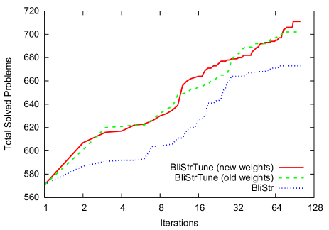
Figure 1: Value added by parameter fine-tuning and by new weight functions (Section 5.1).

To evaluate the hierarchical invention we ran BliStr and BliStrTune with equivalent arguments. Furthermore, we ran two instances of BliStrTune to evaluate the performance added by the new weight functions from Section 2.2. The first instance was allowed to use only the original E 1.9 weight functions, while the second additionally used our new weight functions.

BliStr and BliStrTune used the same input arguments. The first argument is the set of the training problems. We use the 1000 training problems from the Mizar@Turing competition in all experiments. Other arguments are:

$T_{\textit{improve}}$

the time limit (seconds) for one ParamILS run,

$t_{\textit{cutoff}}$

the time limit for E prover runs within ParamILS,

$t_{\textit{eval}}$

the time limit for the protocol evaluation in BliStr/Tune.

In BliStrTune, ParamILS is run four times in each iteration, hence we set $T_{\textit{improve}}=100$ in BliStrTune and $T_{\textit{improve}}=400$ in BliStr.  We set $t_{\textit{cutoff}}=1$ and $t_{\textit{eval}}=5$ and additionally, in the case of BliStrTune, $c_{\textit{cef}}=6$.

The results are shown in Figure 1. In each iteration (x-axis, logarithmic scale) we count the total number of the training problems solved (y-axis) by all the protocols invented so far, provided each protocol is given the time limit $t_{\textit{eval}}$. This metric gives us relatively good idea of the BliStr/Tune progress.

The original BliStr solved 673 problems, BliStrTune without the new weights solved 702 problems, while BliStrTune with the new weights solved 711 problems. From this and from the figure we can see that the greatest improvement is thanks to the hierarchical parameter invention. However, the new weight functions still provide 9 more solved problems which is a useful additional improvement.

5.2 Influence of the BliStrTune Input Arguments

$T_{\textrm{{improve}}}$	$t_{\textrm{{cutoff}}}$	$t_{\textrm{{eval}}}$	$c_{\textit{cef}}$	iters	protos	run time	best proto	solved	useful
100	1	5	6	115	116	1d0h	572	711	28%
100	1	5	10	111	115	1d3h	594	715	14%
300	1	5	6	83	87	1d13h	596	698	4%
300	1	5	10	82	85	1d22h	611	711	11%
100	2	10	6	152	148	1d20h	579	720	27%
100	2	10	10	88	88	1d4h	567	698	1%
300	2	10	6	153	153	3d18h	583	727	19%
300	2	10	10	139	139	3d9h	587	719	15%

Table 1: Evaluation of different BliStrTune training runs on Mizar@Turing problems (Section 5.2).

In this section we evaluate several BliStrTune runs with different input arguments. We run all the combinations of $T_{\textit{improve}}\in\{100,300\}$ and $c_{\textit{cef}}\in\{6,10\}$ and $t_{\textit{cutoff}}\in\{1,2\}$. This gives us 6 different BliStrTune runs. We always set $t_{\textit{eval}}=5\cdot t_{\textit{cutoff}}$.

The results are summarized in Table 1. Column iters contains the number of iterations executed by the appropriate BliStrTune run, proto is the total number of protocols generated, run time is the total run time of the given BliStrTune run, best proto is the number of training problems solved by the best protocol within $t_{\textit{eval}}$ time limit, and solved is the total number of the training problems solved by all the generated protocols, provided each protocol is given time limit $t_{\textit{eval}}$. We can see that a huge amount protocols were generated. Only few of them were used for the final evaluation as described in Section 5.3. Those used for the final evaluation are considered “useful” and the column useful states how many percent of the useful protocols come from the appropriate BliStrTune run.

We can see that the most useful runs are the basic runs with smaller $T_{\textit{improve}}$ which also have lower run times. Higher $T_{\textit{improve}}$ leads to higher run times but it produces better protocols in the sense that a smaller number of protocols can solve equal number of problems. From the table we can see that when $t_{\textit{cutoff}}$ and $c_{\textit{cef}}$ are increased, $T_{\textit{improve}}$ should be increased as well to provide ParamILS enough time for protocol improvement.

5.3 Selecting Best Protocol Scheduler

		training		testing
scheduler	protos	solved	V+	solved	V+
$\text{greedy}_{1}$	33	744	+9.8%	280	+5.2%
$\text{greedy}_{2}$	27	742	+9.6%	279	+4.8%
$\text{greedy}_{5}$	28	734	+8.4%	280	+5.2%
$\text{greedy}_{10}$	22	719	+6.2%	276	+3.8%
$\text{SOTAC}_{15}$	15	663	-2.0%	261	-1.8%
$\text{SOTAC}_{30}$	30	693	+2.3%	266	+0%
$\text{SOTAC}_{45}$	45	698	+3.1%	270	+1.5%
$\text{SOTAC}_{60}$	60	699	+3.2%	270	+1.5%
$\Sigma\text{-SOTAC}_{15}$	15	692	+2.2%	268	+0.7%
$\Sigma\text{-SOTAC}_{30}$	30	711	+5.0%	273	+2.6%
$\Sigma\text{-SOTAC}_{45}$	45	712	+5.1%	276	+3.8%
$\Sigma\text{-SOTAC}_{60}$	60	707	+4.4%	275	+3.4%

Table 2: BliStrTune schedulers evaluation in 60 seconds on Mizar@Turing problems (Section 5.3).

The 6 runs of BliStrTune described above in Section 5.2 generated more than 900 different protocols. In this section we try to select the best subset of protocols and construct a protocol scheduler which sequentially tries several protocols to solve a problem. We only experiment with the simplest schedulers where the time limit for solving a problem is equally distributed among all the protocols within a scheduler. Hence the problem of scheduler construction is reduced to the selection of the right protocols.

We use three different ways to select scheduler protocols. Firstly we use a greedy approach as follows. We evaluate all the protocols on all the training problems with a fixed time limit $t$. Then we construct a greedy covering sequence which starts with the best protocol, and each next protocol in the sequence is the protocol that adds most solutions to the union of problems solved by all previous protocols in the sequence. The resulting scheduler is denoted $\text{greedy}_{t}$.

Second way to construct a scheduler is using state-of-the-art contribution (SOTAC) used by CASC. A SOTAC for the problem is the inverse of the number of protocols that solved the problem. A protocol SOTAC is the average SOTAC over the problems it solves. We can sort the protocols by SOTAC and select first $n$ protocols from this sequence. The resulting scheduler is denoted $\text{SOTAC}_{n}$.

SOTAC of a protocol will be high even if the protocol solves only one problem which no other protocol can solve. That is why also the $\Sigma\text{-SOTAC}$ value Kaliszyk and Urban [2014] is introduced: the sum of problem SOTAC over all the problems. This gives us schedulers denoted $\Sigma\text{-SOTAC}_{n}$.

The evaluation of 12 different schedulers with 60 seconds time limit on the training problems is provided in Table 2. Column protos specifies the count of protocols within the scheduler. We shall use this evaluation to select the best scheduler, hence the results on the 400 testing problems are provided for reference only. Column solved is the number of problems solved in 60s. Column V+ is a percentage gain/lost on a state-of-the-art prover Vampire 4.0 which solves 667 of the 1000 training problems and 266 of the 400 testing problems.

We can see that the best results are achieved by scheduler $\text{greedy}_{1}$, which also gives the best results on the testing problems. Generally, it is better to run a bigger number of protocols with lower individual time limit.

Furthermore, we can use the constructed schedulers to evaluate the contribution of our new weight functions by analyzing weight functions used in the schedulers. Table 4 summarizes the usage of different weight functions in the final schedulers. Our weight functions are referred to by their names from Section 2.2 while the original weights are called by their E prover names. Column count states how many times the corresponding weight function was used in some scheduler protocol, while column freq sums the frequencies of occurrences of CEFs which use the given weight function. We can see that our new weight function Term was the most often used weight function. Four of our weight functions were, however, not used very often which we attribute to their higher time complexity.

5.4 Best Protocol Scheduler Evaluation

	training		testing
prover	solved	V+	solved	V+
E (BliStrTune)	744	+9.8%	280	+5.2%
Vampire 4.0	677	+0%	266	+0%
E (auto-schedule)	605	-10.6%	231	-13.1%

Table 3: Evaluation of the best BliStrTune scheduler on testing problems with 60 seconds time limit.

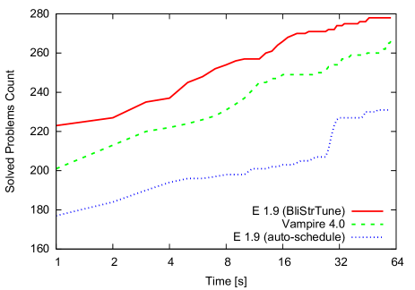
Figure 2: Progress of ATPs on the 400 Mizar@Turing testing problems with 60 seconds time limit.

In this section we evaluate the best protocol scheduler $\text{greedy}_{1}$ selected in previous Section 5.3 on the testing problems with 60 seconds time limit. We compare $\text{greedy}_{1}$ with two state-of-the-art ATPs: (1) with E prover 1.9 in auto-schedule mode and (2) with Vampire 4.0 in CASC mode.

The results are summarized in Table 3. We can see that E with scheduler $\text{greedy}_{1}$ invented by BliStrTune outperforms Vampire by 5.2% and the improvement from E in auto-schedule mode is even more significant. Figure 2 provides a graphical representation of ATP’s progress. For each second (x-axis, logarithmic scale) we count the number of problems solved so far (y-axis). We can see that $\text{greedy}_{1}$ was outperforming Vampire during the whole evaluation.

6 Conclusions and Future Work

In this paper we have described BliStrTune, an extension of a previously published system BliStr, which can be used for hierarchical invention of protocols targeted for a given benchmark problems. The main contribution of BliStrTune is that it considers a much bigger space of protocols by interleaving the global-tuning phase with argument fine-tuning. We have evaluated the original BliStr and our BliStrTune on the same input data and experimentally proved that BliStrTune outperforms BliStr. We have evaluated several ways of creating protocol schedulers and showed that E 1.9 with the best protocol scheduler constructed from BliStrTune protocols targeted for training problems outperforms state-of-the-art ATP Vampire 4.0 on independent testing problems by more than 5%.

Furthermore, we have used BliStrTune to evaluate a contribution of our previously designed weight functions in E prover. We have shown that the new weight functions allow us to solve more problems and that (at least two of them) were often used in the best scheduler protocols. Interestingly, more complex structural weights (like Lev, Ted) were not used very often in the schedulers even though our previous experiments suggested they might be very useful. We attribute this to their higher time complexity and we would like to investigate this in our future research.

Several topics are suggested for future work. We have shown that new weight functions can enhance E prover performance, hence more weight functions which consider term structure could be implemented. It seems that it will be better to design weight functions with lower time complexity, perhaps even providing approximate results (for example, some approximation of the Levenshtein distance which could be computed faster).

Another direction of our future research is to design more complex protocol schedulers. We have achieved good results with the simplest protocol schedulers where each protocol is given an equal amount of time when solving a problem. It would be interesting to design “smarter” schedulers and to see how many more problems can be solved.

Further direction of our future research are enhancements of the BliStr/Tune main loop. We could experiment with settings of various parameters, or with selection of training problems, or we could use parameter improvement methods other than ParamILS Wang et al. [2016]. Finally, we would like to make our implementation easier to use and to distribute it as a solid software package.

weight function	count	freq
Term	111	782
RelevanceLevelWeight2	104	353
Pref	45	297
ConjectureGeneralSymbolWeight	43	235
FIFOWeight	39	174
StaggeredWeight	36	199
SymbolTypeweight	34	96
ConjectureRelativeSymbolWeight	28	110
ConjectureSymbolWeight	23	44
RelevanceLevelWeight	21	40
OrientLMaxWeight	13	24
Refinedweight	12	88
Defaultweight	10	131
Clauseweight	9	64
ClauseWeightAge	6	10
PNRefinedweight	5	21
Struc	5	14
Lev	3	37
Uniqweight	2	2
Ted	1	13
TfIdf	1	1
total	551	2735

Table 4: Usage of weight functions in best schedulers.

Supported by the ERC Consolidator grant number 649043 AI4REASON.

References

- Alama et al. [2014] J. Alama, T. Heskes, D. Kühlwein, E. Tsivtsivadze, and J. Urban. Premise selection for mathematics by corpus analysis and kernel methods. J. Autom. Reasoning, 52(2):191–213, 2014. ISSN 0168-7433. 10.1007/s10817-013-9286-5.
- Blanchette et al. [2016a] J. Blanchette, C. Kaliszyk, L. Paulson, and J. Urban. Hammering towards QED. Journal of Formalized Reasoning, 9(1):101–148, 2016a. ISSN 1972-5787. URL http://jfr.unibo.it/article/view/4593.
- Blanchette et al. [2016b] J. C. Blanchette, D. Greenaway, C. Kaliszyk, D. Kühlwein, and J. Urban. A learning-based fact selector for Isabelle/HOL. J. Autom. Reasoning, 57(3):219–244, 2016b. 10.1007/s10817-016-9362-8. URL http://dx.doi.org/10.1007/s10817-016-9362-8.
- Gauthier and Kaliszyk [2015] T. Gauthier and C. Kaliszyk. Premise selection and external provers for HOL4. In Certified Programs and Proofs (CPP’15), LNCS. Springer, 2015. 10.1145/2676724.2693173. URL http://dx.doi.org/10.1145/2676724.2693173. http://dx.doi.org/10.1145/2676724.2693173.
- Grabowski et al. [2010] A. Grabowski, A. Korniłowicz, and A. Naumowicz. Mizar in a nutshell. J. Formalized Reasoning, 3(2):153–245, 2010.
- Hutter et al. [2009] F. Hutter, H. H. Hoos, K. Leyton-Brown, and T. Stützle. ParamILS: an automatic algorithm configuration framework. J. Artificial Intelligence Research, 36:267–306, October 2009.
- Jakubův and Urban [2016] J. Jakubův and J. Urban. Extending E prover with similarity based clause selection strategies. In Intelligent Computer Mathematics - 9th International Conference, CICM 2016, Bialystok, Poland, July 25-29, 2016, Proceedings, pages 151–156, 2016.
- Kaliszyk and Urban [2014] C. Kaliszyk and J. Urban. Learning-assisted automated reasoning with Flyspeck. J. Autom. Reasoning, 53(2):173–213, 2014. 10.1007/s10817-014-9303-3. URL http://dx.doi.org/10.1007/s10817-014-9303-3.
- Kaliszyk and Urban [2015] C. Kaliszyk and J. Urban. MizAR 40 for Mizar 40. J. Autom. Reasoning, 55(3):245–256, 2015. 10.1007/s10817-015-9330-8. URL http://dx.doi.org/10.1007/s10817-015-9330-8.
- Kaliszyk et al. [2015a] C. Kaliszyk, J. Urban, and J. Vyskocil. Efficient semantic features for automated reasoning over large theories. In Q. Yang and M. Wooldridge, editors, IJCAI’15, pages 3084–3090. AAAI Press, 2015a.
- Kaliszyk et al. [2015b] C. Kaliszyk, J. Urban, and J. Vyskocil. Machine learner for automated reasoning 0.4 and 0.5. In S. Schulz, L. D. Moura, and B. Konev, editors, PAAR-2014. 4th Workshop on Practical Aspects of Automated Reasoning, volume 31 of EPiC Series in Computing, pages 60–66. EasyChair, 2015b.
- Kovács and Voronkov [2013] L. Kovács and A. Voronkov. First-order theorem proving and Vampire. In N. Sharygina and H. Veith, editors, CAV, volume 8044 of LNCS, pages 1–35. Springer, 2013. ISBN 978-3-642-39798-1.
- Kühlwein and Urban [2015] D. Kühlwein and J. Urban. MaLeS: A framework for automatic tuning of automated theorem provers. J. Autom. Reasoning, 55(2):91–116, 2015. 10.1007/s10817-015-9329-1. URL http://dx.doi.org/10.1007/s10817-015-9329-1.
- Leskovec et al. [2014] J. Leskovec, A. Rajaraman, and J. D. Ullman. Mining of Massive Datasets, 2nd Ed. Cambridge University Press, 2014. ISBN 978-1107077232.
- Levenshtein [1966] V. Levenshtein. Binary Codes Capable of Correcting Deletions, Insertions and Reversals. Soviet Physics Doklady, 10:707, 1966.
- McCune [1990] W. McCune. Otter 2.0. In International Conference on Automated Deduction, pages 663–664. Springer, 1990.
- McCune [1989] W. W. McCune. Otter 1. 0 users’ guide. Technical report, Argonne National Lab., IL (USA), 1989.
- McCune [1994] W. W. McCune. Otter 3.0 reference manual and guide, volume 9700. Argonne National Laboratory Argonne, IL, 1994.
- Schäfer and Schulz [2015] S. Schäfer and S. Schulz. Breeding theorem proving heuristics with genetic algorithms. In G. Gottlob, G. Sutcliffe, and A. Voronkov, editors, Global Conference on Artificial Intelligence, GCAI 2015, Tbilisi, Georgia, October 16-19, 2015, volume 36 of EPiC Series in Computing, pages 263–274. EasyChair, 2015. URL http://www.easychair.org/publications/paper/Breeding_Theorem_Proving_Heuristics_with_Genetic_Algorithms.
- Schulz [2002] S. Schulz. E – a brainiac theorem prover. AI Communications, 15(2):111–126, 2002.
- Schulz [2013] S. Schulz. System description: E 1.8. In K. L. McMillan, A. Middeldorp, and A. Voronkov, editors, LPAR, volume 8312 of LNCS, pages 735–743. Springer, 2013. ISBN 978-3-642-45220-8. 10.1007/978-3-642-45221-5_49. URL http://dx.doi.org/10.1007/978-3-642-45221-5_49.
- Sutcliffe [2013] G. Sutcliffe. The 6th IJCAR automated theorem proving system competition - CASC-J6. AI Commun., 26(2):211–223, 2013. 10.3233/AIC-130550. URL http://dx.doi.org/10.3233/AIC-130550.
- Urban [2004] J. Urban. MPTP - Motivation, Implementation, First Experiments. J. Autom. Reasoning, 33(3-4):319–339, 2004. 10.1007/s10817-004-6245-1.
- Urban [2006] J. Urban. MPTP 0.2: Design, implementation, and initial experiments. J. Autom. Reasoning, 37(1-2):21–43, 2006.
- Urban [2015] J. Urban. BliStr: The Blind Strategymaker. In G. Gottlob, G. Sutcliffe, and A. Voronkov, editors, GCAI 2015. Global Conference on Artificial Intelligence, volume 36 of EPiC Series in Computing, pages 312–319. EasyChair, 2015.
- Urban et al. [2008] J. Urban, G. Sutcliffe, P. Pudlák, and J. Vyskočil. MaLARea SG1 - Machine Learner for Automated Reasoning with Semantic Guidance. In A. Armando, P. Baumgartner, and G. Dowek, editors, IJCAR, volume 5195 of LNCS, pages 441–456. Springer, 2008. ISBN 978-3-540-71069-1.
- Wang et al. [2016] Z. Wang, F. Hutter, M. Zoghi, D. Matheson, and N. de Feitas. Bayesian optimization in a billion dimensions via random embeddings. Journal of Artificial Intelligence Research, 55:361–387, 2016.
- Zhang and Shasha [1989] K. Zhang and D. Shasha. Simple fast algorithms for the editing distance between trees and related problems. SIAM J. Comput., 18(6):1245–1262, Dec. 1989. ISSN 0097-5397. 10.1137/0218082. URL http://dx.doi.org/10.1137/0218082.