Bayesian priors and nuisance parameters

Abstract

Bayesian techniques are widely used to obtain spectral functions from correlators. We suggest a technique to rid the results of nuisance parameters, i.e., parameters which are needed for the regularization but cannot be determined from data. We give examples where the method works, including a pion mass extraction with two flavours of staggered quarks at a lattice spacing of about 0.07 fm. We also give an example where the method does not work.

Some years ago, Bayesian techniques were introduced for the analysis of correlation functions obtained in lattice gauge theory at zero bayes and finite tikhonov ; lgtmem temperatures. Although the details required from these analyses differ, there are many similarities. In both cases one needs to analyze measurements of correlation functions, $C(t)$, where $t$ is the separation between the source and sink operators in Euclidean time. The analysis extracts some features of a spectral function, $\rho(\omega)$, where $\omega$ is an “energy” variable. At zero temperature $\rho(\omega)$ is a sum of delta functions, and the locations and strengths of the ones with smallest $\omega$ are interesting. At finite temperature the shape of $\rho(\omega)$ at low $\omega$ is the object of interest. In both cases, the number of features in $\rho(\omega)$ far exceed the number of measurements, and one needs to isolate the features of interest. One may look upon Bayesian techniques as regularization techniques. Bayesian techniques allow us to introduce assumptions about aspects of $\rho(\omega)$, and then to relax some of these assumptions as dictated by data. The procedure involves extraneous (nuisance) parameters, having no physical interpretation, whose treatment remains an open question guber . We address the treatment of these parameters here.

Let us begin with a linear fitting problem, such as the one which arises in the extraction of the spectral function at finite temperature tikhonov . Given a kernel $K$ and the model

$$C(t)=K_{ti}\rho_{i},\qquad(1\leq t\leq N_{t},\;{\rm and}\;1\leq i\leq N_{e}),$$ (1)

we would like to find the optimum values of $\rho_{i}$ which describe a set of data $C(t)$ with covariance matrix $\Sigma$. If the data are scaled by a factor $\lambda$, then the $\rho_{i}$ are also scaled by the same factor.

The familiar case is $N_{t}>N_{e}$. A simple example is to fit a straight line to three points. As we know, are no solutions unless there are linear combinations of the data which do not determine the parameters, as happens if some of the data points are related to each other by adding vectors in the null-space of $K$. If $\Sigma\neq 0$ then one can obtain a consistent solution, even otherwise, by minimizing the norm of $C-K\rho$ using $\Sigma^{-1}$ as a metric. This is the familiar case; the function to be minimized is

$$\chi^{2}(\rho)=\frac{1}{2}\Delta^{T}(\rho)\Sigma^{-1}\Delta(\rho),\qquad{\rm with}\qquad\Delta(\rho)=C-K\rho.$$ (2)

In the space of the parameters $\rho$, the function $\chi^{2}$ is quadratic with no flat directions. Minimizing this corresponds to maximizing the conditional probability of the measurements $C$ given the spectral function $\rho$,

$$P(C|\rho)\propto\exp\left[-\frac{1}{2}\Delta^{T}(\rho)\Sigma^{-1}\Delta(\rho)\right].$$ (3)

The probability arguments are all familiar for Gaussian distributed measurements lyons .

When $N_{t}<N_{e}$ these methods are ill-defined because the data does not constrain the parameters. In other words, the function $\chi^{2}$ has many flat directions. The problem can be regularized if one has a prior guess $\rho^{(0)}$. One includes this by maximizing a probability obtained by using Bayes’ theorem—

$$\frac{\partial P(\rho|C,\rho^{(0)},\alpha)}{\partial\rho_{i}}=0,\qquad{\rm where}\qquad P(\rho|C,\rho^{(0)},\alpha)=\frac{P(C|\rho)P(\rho|\rho^{(0)},\alpha)}{P(C|\rho^{(0)},\alpha)}.$$ (4)

for $P(C|\rho)$ and $P(C|\rho^{(0)},\alpha)$ one uses the expression of eq. (3). The maximum entropy model (MEM) for the new factor is

$$P(\rho|\rho^{(0)},\alpha)\propto\exp\left(\alpha\sum_{i=1}^{N_{e}}\left[\rho_{i}-\rho^{(0)}_{i}-\rho_{i}\log\left(\frac{\rho_{i}}{\rho^{(0)}_{i}}\right)\right]\right).$$ (5)

The parameter $\alpha$ is a nuisance parameter. We can write a real function $f(\rho)=-\log P(\rho|C,\rho^{(0)},\alpha)$, so that the minimization condition reduces to

$$\frac{\partial f(\rho)}{\partial\rho_{i}}=-K_{\mu i}\Sigma^{-1}_{\mu\nu}\Delta_{\nu}(\rho)+\alpha\log\left(\frac{\rho_{i}}{\rho^{(0)}_{i}}\right)=0.$$ (6)

This description of the MEM follows bryan . Similarly, the method of constrained fit (MCF) bayes can be defined by

$$P(\rho|\rho^{(0)},\sigma^{(0)})\propto\exp\left[-\frac{1}{2}\sum_{i=1}^{N_{e}}\left(\frac{\rho_{i}-\rho^{(0)}_{i}}{\sigma^{(0)}_{i}}\right)^{2}\right].$$ (7)

Here the parameters $\sigma^{(0)}_{i}$ are nuisance parameters.

There are several suggestions in the literature on how to treat the MEM nuisance parameter $\alpha$. Note that if we had immense confidence in the prior, then we would replace Bayes’ theorem in eq. (4) by an equation which treats $\alpha$ as a Lagrange multiplier implementing the constraint. However, it is precisely when the prior is not a certainty that interesting things happen, and we allow the data to change our state of knowledge jaynes . Changing $\alpha$ in eq. (5) corresponds to changing the width of $P(\rho|\rho^{(0)})$ around the modal value $\rho^{(0)}$. One suggestion, such as in the first of bayes , is to construct the posterior distribution $P(\alpha|C)$ and then use the most probable $\alpha$. An alternative was suggested in guber that one averages over all values of $\alpha$ with weight $P(\alpha|C)$. This was the procedure followed in lgtmem ; burnier . Although this is consistent with statistical practice for unobserved parameters, the question is whether the degree of confidence in the prior is a normal statistical parameter. Here we examine a different approach to removing the nuisance parameters.

Before proceeding it is worthwhile to consider the nomenclature of nuisance parameters. We have used the term in the sense that these are parameters which cannot be extracted from the measurements at hand. The parameters $\alpha$ in the MEM, or $\sigma^{(0)}_{i}$ in the MCF, quantify confidence limits on the priors. In applications to lattice QCD, they are entirely qualitative, and therefore a nuisance, not to be trusted. However, if these techniques are used to combine multiple data sets, then they are no longer nuisance parameters, but can carry important information. In applications such as detector characterization detector there is no need to remove parameters such as these. One may imagine also that global fits where different experimental data sets are combined, such as neutrino oscillation parameters, CKM matrix analysis, or structure function extractions, could adopt Bayesian treatments where these parameters are used to check consistency of data sets.

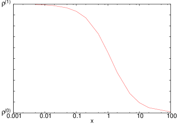
Figure 1: The solution of eq. (10), as a function of $x$, shows a cross over from a region essentially determined by the data, i.e., $\rho=\rho^{(1)}$, to one where it is determined by the prior, i.e., $\rho=\rho^{(0)}$.

Maximum likelihood, i.e., minimizing the $\chi^{2}$ of eq. (2) works when the $N_{t}>N_{e}$. However, nothing prevents us from including a prior into the fit, especially when one is known from other experiments. We develop intuition by understanding this simple case. Take the simplest example, that of fitting a constant to a set of data, so that $N_{e}=1$. A practical application is of extracting a mass from an observation of a flat plateau in local masses. Assume that $\Sigma$ is diagonal. Define

$$d_{2}=\sum_{t=1}^{N_{t}}\frac{C_{t}^{2}}{\sigma_{t}^{2}},\qquad d_{1}=\sum_{\mu=1}^{N_{t}}\frac{C_{t}}{\sigma_{t}^{2}},\qquad d_{0}=\sum_{\mu=1}^{N_{t}}\frac{1}{\sigma_{t}^{2}}.$$ (8)

In this example we will think of $C_{t}$ as local masses, $\sigma_{t}$ as their errors, and $\rho$ to be the estimate of the mass. In the MEM framework, the function to be minimized is

$$f=\frac{d_{0}}{2}\left[\rho^{2}-2\,\frac{d_{1}}{d_{0}}\rho+\frac{d_{2}}{d_{0}}\right]-\alpha\left[\rho-\rho^{(0)}-\rho\log\left(\frac{\rho}{\rho^{(0)}}\right)\right].$$ (9)

Introduce the notation $\rho^{(1)}=d_{1}/d_{0}$ and $x=\alpha/d_{0}$. The minimum occurs at the solution of

$$\rho-\rho^{(1)}=-x\log\left(\frac{\rho}{\rho^{(0)}}\right).$$ (10)

At $x=0$ the prior plays no role, and the solution is the usual maximum likelihood solution $\rho=\rho^{(1)}$. The right hand side vanishes at the prior $\rho=\rho^{(0)}$, and this is the solution when $x\to\infty$. For $x\ll 1$ the solutions remains close to $\rho^{(1)}$ and for $x\gg 1$ it is close to $\rho^{(0)}$, with a cross over between the two regimes occurring when $x\simeq 1$, as shown in Figure 1. When $\alpha=0$ the statistical error, $\sigma$, on the fitted parameter is obtained by solving $f(\rho^{(1)}+\sigma)=f(\rho^{(1)})+1$. This gives $\sigma=\sqrt{2/d_{0}}$. When the prior is included, one could still define the error by the criterion that $f(\rho)$ changes by unity when $\rho$ is changed around the minimum by an amount $\sigma$. One finds that $\sigma$ decreases as $x$ increases, and, in the limit of large $x$, the error $\sigma$ is controlled by the value of $x$. The best fit value and the error then show that the MEM prior determines the fit for large $\alpha$ and the data determines the fit for small $\alpha$, with a cross over between the two regimes when $\alpha\simeq d_{0}$. One expects a similar crossover between prior-driven and data-driven regimes also in MCF.

It was observed recently that the distribution of correlation functions measured in lattice simulations are highly non-Gaussian ilgti . However, it was also shown in that it is possible to analyze this data using modern simulation methods coupled to appropriate bootstrap analysis in such a way that the distribution of local masses, for example, is close enough to Gaussian that the arguments above continue to hold. Even in a non-Gaussian analysis, one may use eq. (6) or its equivalent as a regularization, without using the probability interpretation in eq. (3) or eq. (4).

We explore these methods using the data set used in ilgti . Correlators were measured in two-flavour QCD using staggered quarks. The statistical analysis of the Goldstone pion correlators and local masses are discussed in detail in ilgti . Here we discuss the extraction of a mass from the measured local masses. The quantities to be fitted are a tower of masses, $m_{0}<m_{1}<m_{2}\cdots$ and the corresponding amplitudes $A_{i}$. We chose to analyze the data for $\beta=5.7$ and bare quark mass $ma=0.025$ because it was reported in ilgti that the local mass plateau could was not well developed for this parameter set. This corresponds to a lattice spacing of about 0.07 fm when the scale is set by the Wilson flow scale $w_{0}$. As a result, there was a minor mismatch between the fitted mass and the local masses. It is interesting to do a Bayesian analysis to see whether the lowest mass can be obtained with better confidence.

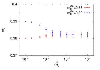
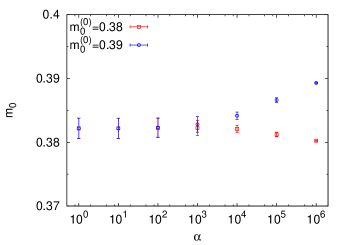
Figure 2: (First panel) The best fit value of $m_{0}$ changes systematically with the nuisance parameter $\sigma^{(0)}_{m_{0}}$ in MCF. For small values of this parameter the best fit to the mass is determined largely by the prior. However, for larger values, the best fit does not depend on $m_{0}^{(0)}$. (Second panel) The dependence on the nuisance parameter $\alpha$ in MEM is the inverse. Both these figures are for the analysis of pion masses at $\beta=5.7$ and bare quark mass $ma=0.025$.

In the MCF we write the prior values $m_{i}^{(0)}$, $A_{i}^{(0)}$, and the nuisance parameters $\sigma^{(0)}_{m_{i}}$ and $\sigma^{(0)}_{A_{i}}$. In the MEM there is a single nuisance parameter $\alpha$. One sees from eq. (5) and eq. (7) that the role played by $\alpha$ is similar to $1/\sigma^{(0)}_{p}$ where $p$ stands for any parameter. We argued above in a particularly simple model that there is a cross over between two kinds of behaviour on tuning $\alpha$: for large $\alpha$ the best fit and its error is determined essentially by the prior, for small $\alpha$ the data determines the fit. In Figure 2 we show that this behaviour is obtained also for a realistic fit.

A similar procedure can be followed for those $m_{i}$ which cannot be fixed by the measurements, and are therefore also nuisance parameters in the same sense as above. For all these parameters we test whether the results for the remaining parameters are stable under change of all the nuisance parameters. Although in principle there is an infinite tower of masses, in practice we found that adding two or three masses was sufficient to give a stable fit for $m_{0}$. We found that $m_{0}$ is measurable, but other masses are not. As a result, the extraction of the ground state mass corresponds to $N_{t}>N_{e}$. Bayesian methods gave an estimate of the mass

$$am_{0}=0.382\pm 0.002\qquad\qquad(\beta=5.7,\ am=0.025,\ N_{f}=2,\ {\rm pion})$$ (11)

which is stable against a variation of all the higher masses we included, their prior confidence limits, the prior value of $m_{0}$, and the prior confidence limit on it, as shown in Figure 2. Exactly the same result is obtained on changing the Bayesian analysis from MEM to MCF. This is to be compared to the value $0.396\pm 0.005$ reported by the simpler analysis in ilgti . In agreement with previous literature, we find that Basyesian analysis can remove the contamination of masses by higher-lying states which dogs the maximum likelihood analysis when the local mass plateau is not fully developed. Our main new technical result remains the observation of a cross over from prior to data dominated regimes in the Bayesian analysis.

We end with a simple cautionary example: fitting a straight line through a single point. This problem with $N_{t}<N_{e}$ is ill-posed without the regularization provided by Bayesian priors. Let us say that we have a measurement of $C(t)$ at $t=1$. The model is $C(t)=a+bt$, with the parameters $a$ and $b$ to be determined. The $1\times 2$ matrix $K$ is given by

$$K=(1\;\;1)=(1)\;(\sqrt{2}\;\;0)\;\left(\begin{matrix}\frac{1}{\sqrt{2}}&\frac{1}{\sqrt{2}}\\ -\,\frac{1}{\sqrt{2}}&\frac{1}{\sqrt{2}}\end{matrix}\right).$$ (12)

where we have also displayed its singular value decomposition (SVD). The null space of $K$ is $a=-b$. If the measurement is $d\pm\sigma$, then $\chi^{2}=(d-a-b)^{2}/\sigma^{2}$. Clearly $a=d$ and $b=0$ is a solution. One can add to it any element from the null space of $K$, i.e., any $a=d+z$ and $b=-z$ is also a solution. The quantity $z$ is completely unconstrained. If we have priors $\rho^{(0)}_{1}=A$ and $\rho^{(0)}_{2}=B$, then the MEM equations are

$$d-a-b=\alpha\sigma^{2}\log\left(\frac{a}{A}\right),\qquad{\rm and}\qquad d-a-b=\alpha\sigma^{2}\log\left(\frac{b}{B}\right).$$ (13)

Now parametrizing $a=A\exp y$, one must also have $b=B\exp y$. The search space is the line $a=(A/B)b$. Along this line the problem becomes well posed,

$$d-(A+B){\rm e}^{y}=\alpha\sigma^{2}y.$$ (14)

For $\alpha=0$ the solution is $a=Ad/(A+B)$ and $b=Bd/(A+B)$. For large $\alpha$ the solution crosses over to the vicinity of the prior $a=A$ and $b=B$. Note that in neither region is the solution independent of the prior. This example shows that even after getting rid of $\alpha$, the best fit parameters may still depend on priors. In this case the Bayesian regulator allows the problem to be solved, but the solution depends on the assumptions. One may immediately see that the problem is structural, and does not depend on the kernel $K$. Since extraction of the spectral function at finite temperature from Euclidean time correlators is a mild generalization of this problem (larger $N_{t}$ and $N_{e}$ and a different $K$), it behooves us to be extremely careful.

In this paper we have examined the Bayesian approach to parameter extraction when all the parameters are not determined by the data. We have shown that some nuisance parameters cause the solution to cross over from a prior dominated to a data dominated region in the best of cases. When this happens, then a reasonable way to deal with the nuisance parameters is to take them to lie in the region where the solution is data driven. However, we have also given an example of a problem where the priors never drop out of the solution. As a result, one must always test the prior-dependence of the Bayesian fits.

Some of the numerical computations used lattice configurations and propagators obtained using the computing resources of the Indian Lattice Gauge Theory Initiative (ILGTI).

References

-
(1)
D. Makovoz, Nucl. Phys. Proc. Suppl. 53 (1997) 246;
G. P. Lepage et al., Nucl. Phys. Proc. Suppl. 106 (2002) 12;
C. Morningstar, Nucl. Phys. Proc. Suppl. 109A (2002) 185. - (2) S. Gupta, Phys. Lett. B 597 (2004) 57 [hep-lat/0301006].
-
(3)
Y. Nakahara, M. Asakawa and T. Hatsuda,
Phys. Rev. D 60 (1999) 091503 [hep-lat/9905034];
T. Yamazaki et al. [CP-PACS Collaboration], Phys. Rev. D 65 (2002) 014501 [hep-lat/0105030];
S. Datta, F. Karsch, P. Petreczky and I. Wetzorke, Phys. Rev. D 69 (2004) 094507 [hep-lat/0312037]. - (4) J. R. Gubernatis et al., Phys. Rev. B 44 (1991) 6011.
- (5) L. Lyons, Statistics for Nuclear and Particle Physicists, Cambridge University Press, 1986.
- (6) R. K. Bryan, Eur. Biophysics J. 18 (1990) 165.
- (7) E. T. Jaynes, Probability Theory, The Logic of Science, ed. G. L. Bretthorst, Cambridge University Press, 2015.
-
(8)
A. Jakovac, P. Petreczky, K. Petrov and A. Velytsky, Phys. Rev.
D 75 (2007) 014506 [hep-lat/0611017];
Y. Burnier and A. Rothkopf, Phys. Rev. Lett. 111 (2013) 182003 [arXiv:1307.6106 [hep-lat]];
G. Aarts, C. Allton, A. Amato, P. Giudice, S. Hands and J. I. Skullerud, JHEP 1502 (2015) 186 [arXiv:1412.6411 [hep-lat]];
H. T. Ding, O. Kaczmarek and F. Meyer, Phys. Rev. D 94 (2016) no.3, 034504 [arXiv:1604.06712 [hep-lat]]. - (9) G. D’Agostini, Nucl. Instrum. Meth. A 362 (1995) 487.
- (10) S. Datta, S. Gupta, A. Lahiri and P. Majumdar, Phys. Rev. D 94 (2016) no.5, 054506 [arXiv:1606.05546 [hep-lat]].