Specific Heat of Spin Excitations Measured by Ferromagnetic Resonance

Abstract

Using ferromagnetic-resonance spectroscopy (FMR), we investigate the anisotropic properties of epitaxial $3\,\mathrm{nm}$Pt/$2\,\mathrm{nm}$Ag/$10\,\mathrm{nm}$Fe/$10\,\mathrm{nm}$Ag/GaAs(001) films in fully saturated meta-stable states at temperatures ranging from $70\,\mathrm{K}$ to $280\,\mathrm{K}$. By comparison to spin-wave theory calculations, we identify the role of thermal fluctuation of magnons in overcoming the energy barrier associated with these meta-stable states. We show that the energy associated with the size of the barrier that bounds the meta-stable regime is proportional to the heat stored in the magnonic bath. Our findings offer the possibility to measure the magnonic contribution to the heat capacity by FMR, independent of other contributions at temperatures ranging from $0\,\mathrm{K}$ to ambient temperature and above. The only requirement being that the selected sample exhibits magnetic anisotropy, here, magnetocrystalline anisotropy.

I Introduction

Knowledge of the magnetic contribution to the thermal properties of physical systems is essential for understanding magnetocalorics(Gutfleisch2011, ), spintronics(Bader2010, ; Chumak2015, ), and magnonic(Chumak2015, ; Serga2014, ) applications. Also, in biomedical applications like hyperthermia (Myrovali2016, ; LiebanaVinas2016, ), it is essential to assess the coupling between the magnetic contributions and the crystal system’s thermal properties. However, measuring the contribution of magnons to the heat capacity of magnetic materials at temperatures of technical interest is challenging. One approach is to suppress magnons by shifting the spin-wave dispersion to energies higher than the thermal energy. The magnon contribution to the total heat can then be separated by conventional calorimetry experiments with and without an applied field. Doing so for a system like Yittrium Iron Garnet (YIG), however, would already require fields as high as $30\,\mathrm{T}$ (Rezende2015, ) at a temperature of only $20\,\mathrm{K}$. Hence, it is unlikely that such experiments can get close to ambient temperature. Another option is to measure the thermal population of the spin-wave dispersion using, for example, Brillouin light scattering (BLS). Here we propose a new method for determining the magnonic heat capacity using ferromagnetic resonance (FMR). Our method is based on ferromagnetic resonance measurements at a fixed frequency, where a magnetic field is applied in different directions near a hard axis of the magnetic anisotropy. First, the magnet is fully saturated, then the direction of the field is swept, such that this saturated configuration becomes metastable all the while FMR is measured at each angle step. We then observe the transition from this metastable configuration to a stable configuration in the FMR signal. From these unconventional FMR measurements, we have evaluated the Zeeman energy in critical configurations of metastable states. We find that in the observed temperature regime between $70\,\mathrm{K}$ and $280\,\mathrm{K}$ the temperature-dependent change of the critical Zeeman energy is proportional to the magnonic heat capacity.

II Experimental procedure

Ferromagnetic resonance measurements were conducted on an epitaxial $3\,\mathrm{nm}$Pt/$2\,\mathrm{nm}$Ag/$10\,\mathrm{nm}$Fe/$10\,\mathrm{nm}$Ag/GaAs(001) thin film in which the (001)-direction of the Fe layer points out of the sample plane. For such systems the Helmholtz free energy density is known to have the form

$$F\left(\vec{B},\vec{M}\right)=-\vec{M}\left(\theta,\phi\right)\cdot\vec{B}\left(\theta_{B},\phi_{B}\right)+\frac{1}{2}\mu_{0}M^{2}\cos^{2}\left(\theta\right)$$ (1)

$$+2K_{2}^{\bot}\sin^{2}\left(\theta\right)+\frac{1}{4}K_{4}\left(\sin^{2}\left(2\theta\right)+\sin^{4}\left(\theta\right)\sin^{2}\left(2\phi\right)\right)$$

including the Zeeman contribution $\vec{M}\cdot\vec{B}$ as discussed in (Farle1998, ). The angles are given in spherical coordinates, where $\theta$ is the polar out-of-plane, and $\phi$ the azimuthal in-plane angle of the magnetization, $\theta_{B}$ and $\phi_{B}$ are the polar and azimuthal angle of the external magnetic field $\vec{B}$ respectively. The anisotropy parameter $K_{4}$ accounts for the cubic magnetocrystalline anisotropy, $K_{2}^{\bot}$ for a uniaxial anisotropy. The thin-film shape-anisotropy is described by the demagnetization term $\frac{1}{2}\mu_{0}M^{2}\cos^{2}\left(\theta\right)$.

For the magnetization to be resonantly excited, $\vec{M}\left(\theta,\phi\right)$ must be a minimizer of this energy landscape. In this case, the magnetization is in an equilibrium state and the resonance condition is described by the curvature of the energy landscape Eq. 1 (Zingsem2017, ). According to (Zingsem2017, ), this holds, even if it is a local minimum. In this case, the equilibrium is metastable, such that the energy landscape presents another - stable - equilibrium. Hence, FMR is expected to occur in metastable states. To create such metastable states in the experiment, we sweep the angle of the applied field at fixed field strengths.

Figure 1: A plot of the energy landscape at different applied field angles for a fixed field magnitude. The black points illustrate the position of the minimum that determines the orientation of the magnetization. Black lines separate the unstable (marked “Un”), metastable (marked “Meta”), and stable (marked “Stable”) regions for this state.

The effect of such an angle sweep on the energy landscape at sufficiently low fields is illustrated in Fig. 1, which shows the in-plane component ($\theta=\theta_{B}=\frac{\pi}{2}$) of the Energy landscape (Eq. 1) as a function of the in-plane angle $\phi$ of the magnetization. First, a magnetic field is applied in an easy direction at $\phi_{B}=0$ (orange curve). Next, the direction of this applied field is changed, i.e., $\phi_{B}$ is increased. Once it is pointing parallel to the hard direction at $\phi_{B}=\frac{\pi}{4}$ (brown curve), two states of equal energy are present. Pushing the angle of the applied field further beyond $\phi_{B}=\frac{\pi}{4}$ makes the state at $\phi<\frac{\pi}{4}$ unfavorable compared to the state at $\phi>\frac{\pi}{4}$. It is now metastable. However, it is still separated from the more favorable state at $\phi>\frac{\pi}{4}$ by an energy barrier. For even larger angles of $\phi_{B}$, the minimum at $\phi<\frac{\pi}{4}$ turns into a saddle point (pink curve) and becomes unstable. The black dots mark the minimum, i.e., the magnetization’s equilibrium alignment for the state at $\phi<\frac{\pi}{4}$.

The experimental procedure for such an angle sweep is schematically shown in Fig. 2. First, a sufficiently large field of $300\,\mathrm{mT}$ is applied along the magnetocrystalline easy axis of the sample to fully align the magnetization and overcome all anisotropies. Then the field is reduced to the desired field value for the angle sweep, and the angle $\phi_{B}$ is swept from the easy axis ($\phi_{B}=0$) across the hard axis ($\phi_{B}=\frac{\pi}{4}$) in steps of $0.1\text{\textdegree}$ to $\phi_{B}=\pi$. One angle step takes about $0.3\,\mathrm{s}$ to measure. During this sweep, the FMR signal is recorded. The sharp discontinuity in the FMR signal, which is indicated as a black line in Fig. 2 b), pinpoints the field-angle configurations at which the magnetization transitions from a metastable to a stable equilibrium. For the applied field magnitudes in this measurement, we find that the transition happens within a few degrees off the hard axis. The dashed curve in Fig. 2 b) shows the points at which the minimum transitions into a saddle-point, i.e., the point at which the metastable equilibrium vanishes. The differentce between the black curve and the dashed curve along the horizontal axis corresponds to the thermal fluctuation field (Bance2014, ).

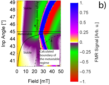
Figure 2: a) Schematic representation of the measurement procedure, using a measured spectrum (compare b) ) for illustration. b) Low field section of the measured FMR signal of a $10\,\mathrm{nm}$ Fe(100) film measured at $9.535\,\mathrm{GHz}$ at room temperature. The straight line at $45\text{\textdegree}$ indicates the magnetocrystalline hard direction. The curved line shows the critical angles at which the metastable regime ends, and the dashed curved line indicates the boundary of the metastable regime as predicted using the theoretical model in ref. (Zingsem2017, ). The difference between the black curve and the dashed curve along the horizontal axis corresponds to the thermal fluctuation field(Bance2014, ).

These measurements were performed at various temperatures, and the curves that follow the measured discontinuities at each temperature are depicted in Fig. 3. With increasing temperature, the discrepancy between the points at which the transition happens, and those at which the metastable state vanishes, becomes larger. Hence, with increasing temperature, the magnetization overcomes larger barriers.

III Results and discussion

We find that, as we decrease the temperature, the critical angle offset from the hard axis at which the magnetization transitions from its metastable into a stable equilibrium increases and approaches the angle predicted for zero temperature, as shown in Fig. 3. The field regime from $20\,\mathrm{mT}$ to $43\,\mathrm{mT}$ was chosen because here, the angles could be well distinguished, and the sample is fully saturated.

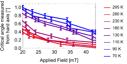
Figure 3: The boundary of the metastable regime for the sample measured in-plane from the hard-axis of the magnetocrystalline anisotropy. Points with error bars represent measured values. Solid lines are linear interpolations used later to determine the temperature derivative at different fields.

For all temperatures, the resonance field was extracted from the FMR spectra, and fitted, solving the commonly used eq. 2 (Farle1998, ; Suhl1955, ; Smit1955, ; Giannopoulos2015, ) to determine the anisotropy parameters.

$$\left(\frac{\omega}{\gamma}\right)^{2}=\frac{1}{M^{2}\sin^{2}\left(\theta\right)}\left(\frac{\mathrm{d}^{2}}{\mathrm{d}\theta^{2}}F\frac{\mathrm{d}^{2}}{\mathrm{d}\phi^{2}}F-\left(\frac{\mathrm{d}^{2}}{\mathrm{d}\theta\mathrm{d}\phi}F\right)^{2}\right)$$ (2)

For the fits, the experimental resonance field was used in the calculation to determine the orientation of the magnetization vector that minimizes the free energy density. This magnetization vector was then used in Eq. 2 to calculate the resonance field position for the respective frequency at a given set of anisotropy parameters. The so determined cubic anisotropy shown in Fig. 4 is in agreement with literature data (Farle1998, ).

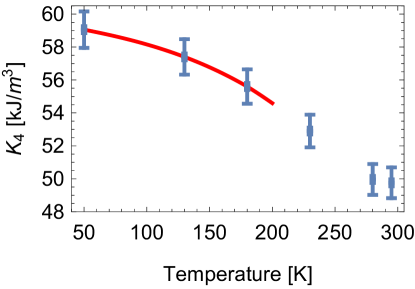
Figure 4: Cubic crystal anisotropy $K_{4}$ as a function of temperature. Blue points with error bars are the values obtained from fitting. The red curve is a third-order polynomial interpolation to serve as a guide to the eye.

The out of plane uniaxial anisotropy $K_{2}^{\bot}$ and the magnetization did not change significantly in the given temperature regime. We obtain $M=(1.71\pm 0.01)\cdot 10^{6}\,\nicefrac{\mathrm{A}}{\mathrm{m}}$ and $K_{2}^{\bot}=(16\pm 0.6)\cdot 10^{3}\,\nicefrac{\mathrm{J}}{\mathrm{m^{3}}}$, using a g-factor of $2.09$(Frait1971, ).

With these values, we then evaluated the contribution of the Zeeman-energy $F_{\mathrm{Zeeman}}=-\vec{M}\cdot\vec{B}$ to the free energy density in Eq. 1 for all temperatures using the critical angles $\phi_{B}$ from Fig. 3 as the in-plane applied field angle. In this calculation, we fixed $\theta_{B}$ and $\theta$ to $90\text{\textdegree}$ as they are constrained by the sample’s shape anisotropy. The magnetization angle $\phi$ is determined numerically by minimization eq. 1 within the metastable regime. This critical Zeeman energy density is the energy density that is provided to the system in order to perform the transition. Therefore we analyze its change as a function of temperature. Considering that the magnetization has some amount of heat available to it in the form of magnons, we would expect that, as we decrease the temperature, more Zeeman energy is required to make the transition. Moreover, since the Zeeman contribution is defined negative, we expect that its change is proportional to the change of the magnon heat in the system. Therefore we calculated the change of the thermal energy of the magnons that is the heat capacity. To calculate the magnonic heat capacity, we proceed as described in (Kittel1963, ). As of (Rezende2014, ) the magnon dispersion can be approximated as

$$\omega\left(k\right)=\gamma B+\omega_{ZB}(1-\cos\left(\frac{\pi}{2}\frac{k}{k_{m}}\right))$$ (3)

where $\gamma$ is the magnetogyric ratio, $B$ is the magnetic flux, $k_{m}=\alpha_{D}\frac{\sqrt[3]{6\pi^{2}}}{a}$ is the radius of the Debye-Sphere with the lattice constant $a$ and the scaling factor $\alpha_{D}$ (Rezende2014a, ) that approximates the Brillouin zone, and $\omega_{ZB}$ is the magnon frequency at the zone boundary. According to (Kittel1963, ), the magnon specific heat can then be written as

$$c_{V}^{\mathrm{magnon}}=\frac{1}{\left(2\pi\right)^{3}}\intop_{0}^{k_{m}}\mathrm{d^{3}}k\frac{\left(\hbar\omega\left(k\right)\right)^{2}}{k_{b}T^{2}}\frac{\exp\left(\frac{\hbar\omega\left(k\right)}{k_{B}T}\right)}{\left(\exp\left(\frac{\hbar\omega\left(k\right)}{k_{B}T}\right)-1\right)^{2}}$$ (4)

by calculating the temperature derivative of the inner energy of the magnons. A comparison between the temperature derivative of the Zeeman contribution and the numerically calculated magnon heat capacity of Fe is shown in Fig. 5. We find that, for each applied field, the curves are proportional and the data is in line with the models in (Wojtczak1983, ) and (Kittel1963, ). This leads us to conclude that this experiment grants direct access to the heat capacity of magnons at elevated temperatures.

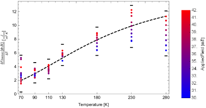
Figure 5: Magnon specific heat as a function of temperature. The red points show the central numerical derivative of the Zeeman contribution to the free energy including error bars. The black dashed curve is the result of numerically evaluating the magnon specific heat eq. 4. The parameters we used for Fe are $a=286.65\,\mathrm{pm}$ (latticFe, ) $\omega_{ZB}=18\,\mathrm{THz}$ (Kittel1963, ) $\gamma=2.92\cdot 10^{10}\,\mathrm{\nicefrac{{1}}{{T\cdot s}}}$ (Frait1971, ) and $\alpha_{D}=0.87$ (Rezende2014a, ).

This technique can be applied to any ferromagnet since any ferromagnet can be tailored to have any desired anisotropy simply by shape, even if the intrinsic magnetocrystalline anisotropy is small.

IV Summary

In a magnetization configuration non-collinear with the external field, we have shown that FMR modes exist in metastable magnetic states as predicted in (Zingsem2017, ). We also find that the magnonic heat capacity of iron is proportional to the temperature derivative of the Zeeman energy at the critical points in the unconventional FMR angular dependence by comparison to spin-wave theory calculations. We find a good agreement between the measured data and the calculation. The magnitude of of the magnon contribution to the specific heat shown in Fig. 5 is also in line with other works(Rezende2014, ; Boona2014, ; Rezende2014a, ; Rezende2015, ). Our results suggest that measuring the temperature-dependent size of the energy barrier, which confines a saturated meta-stable magnetic state, presents a new method for determining the magnon contribution to the specific heat. The only requirement for these measurements is that the sample exhibits magnetic anisotropy. This can either be magnetocrystalline anisotropy or shape anisotropy in patterned magnetic shapes.

- (1) O. Gutfleisch, M. A. Willard, E. Brück, C. H. Chen, S. G. Sankar, and J. P. Liu, “Magnetic materials and devices for the 21st century: Stronger, lighter, and more energy efficient,” Advanced Materials, vol. 23, no. 7, pp. 821–842, 2011. [Online]. Available: https://onlinelibrary.wiley.com/doi/abs/10.1002/adma.201002180
- (2) S. Bader and S. Parkin, “Spintronics,” ARCMP, vol. 1, pp. 71–88, 2010.
- (3) A. V. Chumak, V. I. Vasyuchka, A. A. Serga, and B. Hillebrands, “Magnon spintronics,” Nature Physics, vol. 11, no. 6, pp. 453–461, 2015.
- (4) A. A. Serga, V. S. Tiberkevich, C. W. Sandweg, V. I. Vasyuchka, D. A. Bozhko, A. V. Chumak, T. Neumann, B. Obry, G. A. Melkov, A. N. Slavin et al., “Bose–einstein condensation in an ultra-hot gas of pumped magnons,” Nature communications, vol. 5, no. 1, pp. 1–8, 2014.
- (5) E. Myrovali, N. Maniotis, A. Makridis, A. Terzopoulou, V. Ntomprougkidis, K. Simeonidis, D. Sakellari, O. Kalogirou, T. Samaras, R. Salikhov et al., “Arrangement at the nanoscale: Effect on magnetic particle hyperthermia,” Scientific reports, vol. 6, p. 37934, 2016.
- (6) S. Liébana-Viñas, K. Simeonidis, U. Wiedwald, Z.-A. Li, Z. Ma, E. Myrovali, A. Makridis, D. Sakellari, G. Vourlias, M. Spasova et al., “Optimum nanoscale design in ferrite based nanoparticles for magnetic particle hyperthermia,” Rsc Advances, vol. 6, no. 77, pp. 72 918–72 925, 2016.
- (7) S. M. Rezende and J. C. López Ortiz, “Thermal properties of magnons in yttrium iron garnet at elevated magnetic fields,” Phys. Rev. B, vol. 91, p. 104416, Mar 2015. [Online]. Available: http://link.aps.org/doi/10.1103/PhysRevB.91.104416
- (8) M. Farle, “Ferromagnetic resonance of ultrathin metallic layers,” Reports on Progress in Physics, vol. 61, no. 7, p. 755, 1998. [Online]. Available: http://stacks.iop.org/0034-4885/61/i=7/a=001
- (9) B. W. Zingsem, M. Winklhofer, R. Meckenstock, and M. Farle, “Unified description of collective magnetic excitations,” Phys. Rev. B, vol. 96, p. 224407, Dec 2017. [Online]. Available: https://link.aps.org/doi/10.1103/PhysRevB.96.224407
- (10) S. Bance, H. Oezelt, T. Schrefl, M. Winklhofer, G. Hrkac, G. Zimanyi, O. Gutfleisch, R. F. L. Evans, R. W. Chantrell, T. Shoji, M. Yano, N. Sakuma, A. Kato, and A. Manabe, “High energy product in battenberg structured magnets,” Applied Physics Letters, vol. 105, no. 19, pp. –, 2014. [Online]. Available: http://scitation.aip.org/content/aip/journal/apl/105/19/10.1063/1.4897645
- (11) H. Suhl, “Ferromagnetic resonance in nickel ferrite between one and two kilomegacycles,” Phys. Rev., vol. 97, pp. 555–557, Jan 1955. [Online]. Available: http://link.aps.org/doi/10.1103/PhysRev.97.555.2
- (12) J. Smit and H. G. Beljers, “Ferromagnetic resonance absorption in BaFe12O19, a highly anisotropic crystal,” Philips Research Reports, vol. 10, pp. 113–130, 1955.
- (13) G. Giannopoulos, R. Salikhov, B. Zingsem, A. Markou, I. Panagiotopoulos, V. Psycharis, M. Farle, and D. Niarchos, “Large magnetic anisotropy in strained Fe/Co multilayers on AuCu and the effect of carbon doping,” APL Mater., vol. 3, no. 4, pp. –, 2015. [Online]. Available: http://scitation.aip.org/content/aip/journal/aplmater/3/4/10.1063/1.4919058
- (14) Z. Frait and R. Gemperle, “The g-factor and surface magnetization of pure iron along [100] and [111] directions,” Le Journal de Physique Colloques, vol. 32, no. C1, pp. C1–541, 1971.
- (15) C. Kittel, Quantum theory of solids. New York: Wiley, 1963.
- (16) S. M. Rezende, R. L. Rodríguez-Suárez, R. O. Cunha, A. R. Rodrigues, F. L. A. Machado, G. A. Fonseca Guerra, J. C. Lopez Ortiz, and A. Azevedo, “Magnon spin-current theory for the longitudinal spin-seebeck effect,” Phys. Rev. B, vol. 89, p. 014416, Jan 2014. [Online]. Available: http://link.aps.org/doi/10.1103/PhysRevB.89.014416
- (17) S. M. Rezende, R. L. Rodríguez-Suárez, J. C. Lopez Ortiz, and A. Azevedo, “Thermal properties of magnons and the spin seebeck effect in yttrium iron garnet/normal metal hybrid structures,” Phys. Rev. B, vol. 89, p. 134406, Apr 2014. [Online]. Available: http://link.aps.org/doi/10.1103/PhysRevB.89.134406
- (18) L. Wojtczak, A. Urbaniak-Kucharczyk, J. Mielnicki, and B. Mrygon, “The magnetic contribution to specific heat in thin ferromagnetic films,” physica status solidi (a), vol. 76, no. 1, pp. 113–120, 1983. [Online]. Available: https://onlinelibrary.wiley.com/doi/abs/10.1002/pssa.2210760112
- (19) P. Kohlhaas, R. Donner and N. Schmitz-Pranghe, “Über die temperaturabhangigkeit der gitterparameter von eisen, kobalt und nickel im bereich hoher temperaturen,” Z. Angew. Phys., vol. 23, pp. 245–249, 1967.
- (20) S. R. Boona and J. P. Heremans, “Magnon thermal mean free path in yttrium iron garnet,” Physical Review B, vol. 90, no. 6, p. 064421, 2014.