Reliability of k-out-of-n Data Storage System with Deterministic Parallel and Serial Repair

Vaneet Aggarwal V. Aggarwal is with the School of IE, Purdue University, email: vaneet@purdue.edu
Abstract

In this paper, we find the Laplace Stieltjes transform of the probability of data loss for the k-out-of-n distributed storage system with deterministic repair times. We consider two repair models, namely the serial and parallel repair. We show that for failure rate much lower than the repair rate, mean time of data loss for the two models is the same unlike the case for exponential repair models.

Index Terms:
k-out-of-n storage systems, parallel repair, serial repair, reliability, mean time to data loss

I Introduction

Data storage demands have been increasing very rapidly, leading to a lot of interest in distributed storage systems [1, 2]. Erasure-coded distributed storage systems provide reliable data storage at a a fraction of the cost as compared to the systems based on simple data replication. Characterizing the reliability of the storage system is an important problem. Reliability has been explored for exponential repair times for serial repair [3] and parallel repair [4] models. Recently, there has been interest to characterize the reliability for deterministc repair times [7, 8], where geometric interpretations are provided. However, there is no complete characterization of reliability for parallel and serial repair models. The authors of [5] considers availability of the k-out-of-n systems with general repair times while this paper considers the reliability of k-out-of-n systems. In this paper, we give the Laplace Stieltjes transform of the probability of data loss for both parallel and serial repair models.

Using the Laplace Stieltjes Transform formulas, mean time to data loss can be found. Even though expressions are difficult to evaluate exactly, we can find the dominant terms for the case when repair rate is much higher than the failure rate and find that the dominant term for the serial repair is the same as in the case of exponential repair in [3]. However, we also find that the parallel repair also gives the same dominant term as the serial repair, and thus not achieving the $(n-k)!$ factor improvement in mean time to data loss as given in [4] for the parallel exponential repair. The results are compared in simulations, where we see that the mean time to data loss with parallel repair is higher, but the asymptote as the repair rate increases is the same.

The rest of the paper is organized as follows. In Section 2, we give our results for the serial repair model. Section 3 presents our results for the parallel repair model. Section 4 gives the numerical results and Section 5 concludes this paper.

II Serial Repair Model

The serial repair model can be described with the following assumptions.

  1. 1.

    $n>0$ components (disks) are identical and independent.

  2. 2.

    The failure rate for each disk is constant, and equals $\lambda$ (failure time is exponentially distributed for each disk).

  3. 3.

    The repair times are independent and fixed, and equals $t_{rep}$.

  4. 4.

    The repair for the previous broken components must be re-initialized when a new component fails, and only the newest broken component is repaired.

  5. 5.

    The system stops working when $n-k+1$ components have failed for $0<k<n$, $k,n\in{\mathbb{Z}}$.

Suppose that the probability of data loss in time $t$ is $P_{c}(t)$. Then the Laplace Stieltjes Transform of reliability is given as $P_{c}(s)={\mathbb{E}}[e^{-sT}]$, where $T$ is the random variable representing the time to data loss, and $P_{c}(t)=\Pr(T\leq t)$. The next result gives the Laplace Stieltjes Transform of reliability for serial repair.

Theorem 1.

The Laplace Stieltjes Transform of reliability for serial repair is given by

Pc​(s)=Q0,1βˆ—β€‹(s)​Q1,2βˆ—β€‹(s)​Q2,3βˆ—β€‹(s)​⋯​Qnβˆ’k,nβˆ’k+1βˆ—β€‹(s)det([1βˆ’Q0,1βˆ—β€‹(s)0β‹―000βˆ’Q1,0βˆ—β€‹(s)1βˆ’Q1,2βˆ—β€‹(s)β‹―000β‹―β‹―000β‹―βˆ’Qnβˆ’kβˆ’1,nβˆ’kβˆ’2βˆ—β€‹(s)1βˆ’Qnβˆ’kβˆ’1,nβˆ’kβˆ—β€‹(s)000β‹―0βˆ’Qnβˆ’k,nβˆ’kβˆ’1βˆ—β€‹(s)1])subscript𝑃𝑐𝑠superscriptsubscript𝑄01𝑠superscriptsubscript𝑄12𝑠superscriptsubscript𝑄23𝑠⋯superscriptsubscriptπ‘„π‘›π‘˜π‘›π‘˜1𝑠matrix1superscriptsubscript𝑄01𝑠0β‹―000superscriptsubscript𝑄10𝑠1superscriptsubscript𝑄12𝑠⋯000β‹―β‹―000β‹―superscriptsubscriptπ‘„π‘›π‘˜1π‘›π‘˜2𝑠1superscriptsubscriptπ‘„π‘›π‘˜1π‘›π‘˜π‘ 000β‹―0superscriptsubscriptπ‘„π‘›π‘˜π‘›π‘˜1𝑠1\displaystyle P_{c}(s)=\frac{Q_{0,1}^{*}(s)Q_{1,2}^{*}(s)Q_{2,3}^{*}(s)\cdots Q_{n-k,n-k+1}^{*}(s)}{\det\left(\begin{bmatrix}1&-Q_{0,1}^{*}(s)&0&\cdots&0&0&0\\ -Q_{1,0}^{*}(s)&1&-Q_{1,2}^{*}(s)&\cdots&0&0&0\\ \cdots\\ \cdots\\ 0&0&0&\cdots&-Q_{n-k-1,n-k-2}^{*}(s)&1&-Q_{n-k-1,n-k}^{*}(s)\\ 0&0&0&\cdots&0&-Q_{n-k,n-k-1}^{*}(s)&1\end{bmatrix}\right)},

(1)

where

Qi​jβˆ—β€‹(s)={n​λs+n​λ if ​i=0,j=1(nβˆ’i)​λ(nβˆ’i)​λ+s​(1βˆ’eβˆ’((nβˆ’i)​λ+s)​tr​e​p)Β if ​j=i+1,1≀i≀nβˆ’keβˆ’((nβˆ’i)​λ+s)​tr​e​pΒ if ​j=iβˆ’1,1≀i≀nβˆ’k0Β otherwisesuperscriptsubscript𝑄𝑖𝑗𝑠casesπ‘›πœ†π‘ π‘›πœ†formulae-sequenceΒ if 𝑖0𝑗1π‘›π‘–πœ†π‘›π‘–πœ†π‘ 1superscriptπ‘’π‘›π‘–πœ†π‘ subscriptπ‘‘π‘Ÿπ‘’π‘formulae-sequenceΒ if 𝑗𝑖11π‘–π‘›π‘˜superscriptπ‘’π‘›π‘–πœ†π‘ subscriptπ‘‘π‘Ÿπ‘’π‘formulae-sequenceΒ if 𝑗𝑖11π‘–π‘›π‘˜0Β otherwiseQ_{ij}^{*}(s)=\begin{cases}\frac{n\lambda}{s+n\lambda}&\text{ if }i=0,j=1\\ \frac{(n-i)\lambda}{(n-i)\lambda+s}(1-e^{-((n-i)\lambda+s)t_{rep}})&\text{ if }j=i+1,1\leq i\leq n-k\\ e^{-((n-i)\lambda+s)t_{rep}}&\text{ if }j=i-1,1\leq i\leq n-k\\ 0&\text{ otherwise}\end{cases} (2)
Proof.

Let $Q_{ij}(t)$ be the one-step transition probability from state $i$ to state $j$ in time $t$, in which one-step implies that there is only one repair or failure during an interval of time $t$. Then, $Q_{ij}(t)$ is given as

$$Q_{ij}(t)=\begin{cases}\int_{x=0}^{t}n\lambda e^{-n\lambda x}dx&\text{ if }i=0,j=1\\ \int_{x=0}^{\min(t,t_{rep})}(n-i)\lambda e^{-(n-i)\lambda x}dx&\text{ if }j=i+1,1\leq i\leq n-k\\ \int_{x=0}^{t}e^{-(n-i)\lambda t_{rep}}\delta(x=t_{rep})dx&\text{ if }j=i-1,1\leq i\leq n-k\\ 0&\text{ otherwise}\end{cases}$$ (3)

The Laplace-Stieltjes transform is given by

Qi​jβˆ—β€‹(s)={n​λs+n​λ if ​i=0,j=1(nβˆ’i)​λ(nβˆ’i)​λ+s​(1βˆ’eβˆ’((nβˆ’i)​λ+s)​tr​e​p)Β if ​j=i+1,1≀i≀nβˆ’keβˆ’((nβˆ’i)​λ+s)​tr​e​pΒ if ​j=iβˆ’1,1≀i≀nβˆ’k0Β otherwisesuperscriptsubscript𝑄𝑖𝑗𝑠casesπ‘›πœ†π‘ π‘›πœ†formulae-sequenceΒ if 𝑖0𝑗1π‘›π‘–πœ†π‘›π‘–πœ†π‘ 1superscriptπ‘’π‘›π‘–πœ†π‘ subscriptπ‘‘π‘Ÿπ‘’π‘formulae-sequenceΒ if 𝑗𝑖11π‘–π‘›π‘˜superscriptπ‘’π‘›π‘–πœ†π‘ subscriptπ‘‘π‘Ÿπ‘’π‘formulae-sequenceΒ if 𝑗𝑖11π‘–π‘›π‘˜0Β otherwiseQ_{ij}^{*}(s)=\begin{cases}\frac{n\lambda}{s+n\lambda}&\text{ if }i=0,j=1\\ \frac{(n-i)\lambda}{(n-i)\lambda+s}(1-e^{-((n-i)\lambda+s)t_{rep}})&\text{ if }j=i+1,1\leq i\leq n-k\\ e^{-((n-i)\lambda+s)t_{rep}}&\text{ if }j=i-1,1\leq i\leq n-k\\ 0&\text{ otherwise}\end{cases} (4)

Let $H_{ij}(t)$ be the first recurrence time from state $i$ to state $j$. Then, $H_{ij}(t)$ is given as

Hi​j​(t)=Qi​j​(t)+βˆ‘mβ‰ j∫x=0tHm,j​(tβˆ’x)​𝑑Qi,m​(x)subscript𝐻𝑖𝑗𝑑subscript𝑄𝑖𝑗𝑑subscriptπ‘šπ‘—superscriptsubscriptπ‘₯0𝑑subscriptπ»π‘šπ‘—π‘‘π‘₯differential-dsubscriptπ‘„π‘–π‘šπ‘₯H_{ij}(t)=Q_{ij}(t)+\sum_{m\neq j}\int_{x=0}^{t}H_{m,j}(t-x)dQ_{i,m}(x) (5)

The Laplace-Stieltjes transform is then given by

Hi​jβˆ—β€‹(s)=Qi​jβˆ—β€‹(s)+βˆ‘mβ‰ jHm,jβˆ—β€‹(s)​Qi,mβˆ—β€‹(s)superscriptsubscript𝐻𝑖𝑗𝑠superscriptsubscript𝑄𝑖𝑗𝑠subscriptπ‘šπ‘—superscriptsubscriptπ»π‘šπ‘—π‘ superscriptsubscriptπ‘„π‘–π‘šπ‘ H_{ij}^{*}(s)=Q_{ij}^{*}(s)+\sum_{m\neq j}H_{m,j}^{*}(s)Q_{i,m}^{*}(s) (6)

The above can be used to write

[H0,nβˆ’k+1βˆ—β€‹(s)H1,nβˆ’k+1βˆ—β€‹(s)H2,nβˆ’k+1βˆ—β€‹(s)β‹―Hnβˆ’kβˆ’2,nβˆ’k+1βˆ—β€‹(s)Hnβˆ’kβˆ’1,nβˆ’k+1βˆ—β€‹(s)Hnβˆ’k,nβˆ’k+1βˆ—β€‹(s)]=[0Q0,1βˆ—β€‹(s)0β‹―000Q1,0βˆ—β€‹(s)0Q1,2βˆ—β€‹(s)β‹―000β‹―β‹―000β‹―Qnβˆ’kβˆ’1,nβˆ’kβˆ’2βˆ—β€‹(s)0Qnβˆ’kβˆ’1,nβˆ’kβˆ—β€‹(s)000β‹―0Qnβˆ’k,nβˆ’kβˆ’1βˆ—β€‹(s)0]​[H0,nβˆ’k+1βˆ—β€‹(s)H1,nβˆ’k+1βˆ—β€‹(s)H2,nβˆ’k+1βˆ—β€‹(s)β‹―Hnβˆ’kβˆ’2,nβˆ’k+1βˆ—β€‹(s)Hnβˆ’kβˆ’1,nβˆ’k+1βˆ—β€‹(s)Hnβˆ’k,nβˆ’k+1βˆ—β€‹(s)]+[000β‹―00Qnβˆ’k,nβˆ’k+1βˆ—β€‹(s)]matrixsuperscriptsubscript𝐻0π‘›π‘˜1𝑠superscriptsubscript𝐻1π‘›π‘˜1𝑠superscriptsubscript𝐻2π‘›π‘˜1𝑠⋯superscriptsubscriptπ»π‘›π‘˜2π‘›π‘˜1𝑠superscriptsubscriptπ»π‘›π‘˜1π‘›π‘˜1𝑠superscriptsubscriptπ»π‘›π‘˜π‘›π‘˜1𝑠matrix0superscriptsubscript𝑄01𝑠0β‹―000superscriptsubscript𝑄10𝑠0superscriptsubscript𝑄12𝑠⋯000β‹―β‹―000β‹―superscriptsubscriptπ‘„π‘›π‘˜1π‘›π‘˜2𝑠0superscriptsubscriptπ‘„π‘›π‘˜1π‘›π‘˜π‘ 000β‹―0superscriptsubscriptπ‘„π‘›π‘˜π‘›π‘˜1𝑠0matrixsuperscriptsubscript𝐻0π‘›π‘˜1𝑠superscriptsubscript𝐻1π‘›π‘˜1𝑠superscriptsubscript𝐻2π‘›π‘˜1𝑠⋯superscriptsubscriptπ»π‘›π‘˜2π‘›π‘˜1𝑠superscriptsubscriptπ»π‘›π‘˜1π‘›π‘˜1𝑠superscriptsubscriptπ»π‘›π‘˜π‘›π‘˜1𝑠matrix000β‹―00superscriptsubscriptπ‘„π‘›π‘˜π‘›π‘˜1𝑠\displaystyle\begin{bmatrix}H_{0,n-k+1}^{*}(s)\\ H_{1,n-k+1}^{*}(s)\\ H_{2,n-k+1}^{*}(s)\\ \cdots\\ H_{n-k-2,n-k+1}^{*}(s)\\ H_{n-k-1,n-k+1}^{*}(s)\\ H_{n-k,n-k+1}^{*}(s)\end{bmatrix}=\begin{bmatrix}0&Q_{0,1}^{*}(s)&0&\cdots&0&0&0\\ Q_{1,0}^{*}(s)&0&Q_{1,2}^{*}(s)&\cdots&0&0&0\\ \cdots\\ \cdots\\ 0&0&0&\cdots&Q_{n-k-1,n-k-2}^{*}(s)&0&Q_{n-k-1,n-k}^{*}(s)\\ 0&0&0&\cdots&0&Q_{n-k,n-k-1}^{*}(s)&0\end{bmatrix}\begin{bmatrix}H_{0,n-k+1}^{*}(s)\\ H_{1,n-k+1}^{*}(s)\\ H_{2,n-k+1}^{*}(s)\\ \cdots\\ H_{n-k-2,n-k+1}^{*}(s)\\ H_{n-k-1,n-k+1}^{*}(s)\\ H_{n-k,n-k+1}^{*}(s)\end{bmatrix}+\begin{bmatrix}0\\ 0\\ 0\\ \cdots\\ 0\\ 0\\ Q_{n-k,n-k+1}^{*}(s)\end{bmatrix}

(7)

Let $P_{i}(t)$ be the probability that the system is at state $i$ at time $t$ starting from state 00 at time $t=0$, and let $P_{i}^{*}(s)$ be the Laplace-Steiltjes transform. Then, the probability of data loss is given by $P_{n-k+1}(t)=H_{0,n-k+1}(t)$. Thus, it is enough to find $H_{0,n-k+1}(t)$. From Equation (7), we have

H0,nβˆ’k+1βˆ—β€‹(s)=Q0,1βˆ—β€‹(s)​Q1,2βˆ—β€‹(s)​Q2,3βˆ—β€‹(s)​⋯​Qnβˆ’k,nβˆ’k+1βˆ—β€‹(s)det([1βˆ’Q0,1βˆ—β€‹(s)0β‹―000βˆ’Q1,0βˆ—β€‹(s)1βˆ’Q1,2βˆ—β€‹(s)β‹―000β‹―β‹―000β‹―βˆ’Qnβˆ’kβˆ’1,nβˆ’kβˆ’2βˆ—β€‹(s)1βˆ’Qnβˆ’kβˆ’1,nβˆ’kβˆ—β€‹(s)000β‹―0βˆ’Qnβˆ’k,nβˆ’kβˆ’1βˆ—β€‹(s)1])superscriptsubscript𝐻0π‘›π‘˜1𝑠superscriptsubscript𝑄01𝑠superscriptsubscript𝑄12𝑠superscriptsubscript𝑄23𝑠⋯superscriptsubscriptπ‘„π‘›π‘˜π‘›π‘˜1𝑠matrix1superscriptsubscript𝑄01𝑠0β‹―000superscriptsubscript𝑄10𝑠1superscriptsubscript𝑄12𝑠⋯000β‹―β‹―000β‹―superscriptsubscriptπ‘„π‘›π‘˜1π‘›π‘˜2𝑠1superscriptsubscriptπ‘„π‘›π‘˜1π‘›π‘˜π‘ 000β‹―0superscriptsubscriptπ‘„π‘›π‘˜π‘›π‘˜1𝑠1\displaystyle H_{0,n-k+1}^{*}(s)=\frac{Q_{0,1}^{*}(s)Q_{1,2}^{*}(s)Q_{2,3}^{*}(s)\cdots Q_{n-k,n-k+1}^{*}(s)}{\det\left(\begin{bmatrix}1&-Q_{0,1}^{*}(s)&0&\cdots&0&0&0\\ -Q_{1,0}^{*}(s)&1&-Q_{1,2}^{*}(s)&\cdots&0&0&0\\ \cdots\\ \cdots\\ 0&0&0&\cdots&-Q_{n-k-1,n-k-2}^{*}(s)&1&-Q_{n-k-1,n-k}^{*}(s)\\ 0&0&0&\cdots&0&-Q_{n-k,n-k-1}^{*}(s)&1\end{bmatrix}\right)}

(8)

∎

Using $P_{c}(s)$, we can find the mean time to data loss as $-P_{c}^{\prime}(0)$. Given the exact expression of $P_{c}(s)$, we can evaluate $-P_{c}^{\prime}(0)$. However, the expression is cumbersome and thus omitted. We consider however the scenario where $\lambda t_{rep}<<1$ and give the mean time to data loss in that scenario.

Corollary 1.

The mean time to data loss for serial deterministic repair for $\lambda t_{rep}<<1$ is approximately given as

$${\text{MTDL}}_{c}\approx\frac{(k-1)!}{n!\lambda}\frac{1}{(\lambda t_{rep})^{n-k}}$$ (9)
Proof.

The proof follows by using expression for $-P_{c}^{\prime}(0)$ and ignoring all terms of lower order. The detailed steps are omitted. ∎

We note that for exponential serial repair model with rate of repair $\mu$, mean time to data loss was characterized in [6], and is given as

$${\text{MTDL}}_{Chen}=\sum_{l=0}^{n-k}\frac{1}{(n-l)!}\sum_{i=0}^{n-k-l}\mu^{i}\lambda^{-(i+1)}(n-l-i-1)!,$$ (10)

with an approximation given as [3]

$${\text{MTDL}}_{Chen}\approx\frac{(k-1)!}{n!}\frac{\mu^{n-k}}{\lambda^{n-k+1}}.$$ (11)

We note that the MTDL approximation for serial repair with deterministic repair is the same as the approximation with exponential repair for $t_{rep}=1/\mu$.

III Parallel Repair Model

The parallel repair model can be described with the following assumptions.

  1. 1.

    $n>0$ components (disks) are identical and independent.

  2. 2.

    The failure rate for each disk is constant, and equals $\lambda$ (failure time is exponentially distributed for each disk).

  3. 3.

    The repair times are independent and fixed, and equals $t_{rep}$.

  4. 4.

    The repair for the previous broken components must be re-initialized when a new component fails, and all the broken components are simultaneously repaired.

  5. 5.

    The system stops working when $n-k+1$ components have failed for $0<k<n$, $k,n\in{\mathbb{Z}}$.

Suppose that the probability of data loss in time $t$ is $P_{a}(t)$. Then the Laplace Stieltjes Transform of reliability is given as Pa​(s)=𝔼​[eβˆ’s​T]subscriptπ‘ƒπ‘Žπ‘ π”Όdelimited-[]superscript𝑒𝑠𝑇P_{a}(s)={\mathbb{E}}[e^{-sT}], where $T$ is the random variable representing the time to data loss, and $P_{a}(t)=\Pr(T\leq t)$. The next result gives the Laplace Stieltjes Transform of reliability for parallel repair.

Theorem 2.

The Laplace Stieltjes Transform of reliability for parallel repair is given by

Pa​(s)=Q0,1βˆ—β€‹(s)​Q1,2βˆ—β€‹(s)​Q2,3βˆ—β€‹(s)​⋯​Qnβˆ’k,nβˆ’k+1βˆ—β€‹(s)det([1βˆ’Q0,1βˆ—β€‹(s)0β‹―000βˆ’Q1,0βˆ—β€‹(s)1βˆ’Q1,2βˆ—β€‹(s)β‹―000β‹―β‹―βˆ’Qnβˆ’kβˆ’1,0βˆ—β€‹(s)00β‹―01βˆ’Qnβˆ’kβˆ’1,nβˆ’kβˆ—β€‹(s)βˆ’Qnβˆ’k,0βˆ—β€‹(s)00β‹―001])subscriptπ‘ƒπ‘Žπ‘ superscriptsubscript𝑄01𝑠superscriptsubscript𝑄12𝑠superscriptsubscript𝑄23𝑠⋯superscriptsubscriptπ‘„π‘›π‘˜π‘›π‘˜1𝑠matrix1superscriptsubscript𝑄01𝑠0β‹―000superscriptsubscript𝑄10𝑠1superscriptsubscript𝑄12𝑠⋯000β‹―β‹―superscriptsubscriptπ‘„π‘›π‘˜10𝑠00β‹―01superscriptsubscriptπ‘„π‘›π‘˜1π‘›π‘˜π‘ superscriptsubscriptπ‘„π‘›π‘˜0𝑠00β‹―001\displaystyle P_{a}(s)=\frac{Q_{0,1}^{*}(s)Q_{1,2}^{*}(s)Q_{2,3}^{*}(s)\cdots Q_{n-k,n-k+1}^{*}(s)}{\det\left(\begin{bmatrix}1&-Q_{0,1}^{*}(s)&0&\cdots&0&0&0\\ -Q_{1,0}^{*}(s)&1&-Q_{1,2}^{*}(s)&\cdots&0&0&0\\ \cdots\\ \cdots\\ -Q_{n-k-1,0}^{*}(s)&0&0&\cdots&0&1&-Q_{n-k-1,n-k}^{*}(s)\\ -Q_{n-k,0}^{*}(s)&0&0&\cdots&0&0&1\end{bmatrix}\right)},

(12)

where

Qi​jβˆ—β€‹(s)={n​λs+n​λ if ​i=0,j=1(nβˆ’i)​λ(nβˆ’i)​λ+s​(1βˆ’eβˆ’((nβˆ’i)​λ+s)​tr​e​p)Β if ​j=i+1,1≀i≀nβˆ’keβˆ’((nβˆ’i)​λ+s)​tr​e​pΒ if ​j=0,1≀i≀nβˆ’k0Β otherwisesuperscriptsubscript𝑄𝑖𝑗𝑠casesπ‘›πœ†π‘ π‘›πœ†formulae-sequenceΒ if 𝑖0𝑗1π‘›π‘–πœ†π‘›π‘–πœ†π‘ 1superscriptπ‘’π‘›π‘–πœ†π‘ subscriptπ‘‘π‘Ÿπ‘’π‘formulae-sequenceΒ if 𝑗𝑖11π‘–π‘›π‘˜superscriptπ‘’π‘›π‘–πœ†π‘ subscriptπ‘‘π‘Ÿπ‘’π‘formulae-sequenceΒ if 𝑗01π‘–π‘›π‘˜0Β otherwiseQ_{ij}^{*}(s)=\begin{cases}\frac{n\lambda}{s+n\lambda}&\text{ if }i=0,j=1\\ \frac{(n-i)\lambda}{(n-i)\lambda+s}(1-e^{-((n-i)\lambda+s)t_{rep}})&\text{ if }j=i+1,1\leq i\leq n-k\\ e^{-((n-i)\lambda+s)t_{rep}}&\text{ if }j=0,1\leq i\leq n-k\\ 0&\text{ otherwise}\end{cases} (13)

The above can be simplified to

Pa​(s)=Q0,1βˆ—β€‹(s)​Q1,2βˆ—β€‹(s)​Q2,3βˆ—β€‹(s)​⋯​Qnβˆ’k,nβˆ’k+1βˆ—β€‹(s)1βˆ’βˆ‘j=1nβˆ’k((Ξ i=0jβˆ’1​Qi,i+1βˆ—β€‹(s))​Qj,0βˆ—β€‹(s)).subscriptπ‘ƒπ‘Žπ‘ superscriptsubscript𝑄01𝑠superscriptsubscript𝑄12𝑠superscriptsubscript𝑄23𝑠⋯superscriptsubscriptπ‘„π‘›π‘˜π‘›π‘˜1𝑠1superscriptsubscript𝑗1π‘›π‘˜superscriptsubscriptΠ𝑖0𝑗1superscriptsubscript𝑄𝑖𝑖1𝑠superscriptsubscript𝑄𝑗0𝑠P_{a}(s)=\frac{Q_{0,1}^{*}(s)Q_{1,2}^{*}(s)Q_{2,3}^{*}(s)\cdots Q_{n-k,n-k+1}^{*}(s)}{1-\sum_{j=1}^{n-k}\left((\Pi_{i=0}^{j-1}Q_{i,i+1}^{*}(s))Q_{j,0}^{*}(s)\right)}. (14)
Proof.

The proof steps are very similar to that for serial repair model, where the difference is that all the failed components get repaired simultaneously thus going from State i to State 0 on repair rather than to State i-1 for the serial repair model. ∎

Using Pa​(s)subscriptπ‘ƒπ‘Žπ‘ P_{a}(s), we can find the mean time to data loss as $-P_{a}^{\prime}(0)$. Given the exact expression of Pa​(s)subscriptπ‘ƒπ‘Žπ‘ P_{a}(s), we can evaluate $-P_{a}^{\prime}(0)$. However, the expression is cumbersome and thus omitted. We consider however the scenario where $\lambda t_{rep}<<1$ and give the mean time to data loss in that scenario.

Corollary 2.

The mean time to data loss for parallel deterministic repair for $\lambda t_{rep}<<1$ is approximately given as

$${\text{MTDL}}_{a}\approx\frac{(k-1)!}{n!\lambda}\frac{1}{(\lambda t_{rep})^{n-k}}$$ (15)
Proof.

The proof follows by using expression for $-P_{a}^{\prime}(0)$ and ignoring all terms of lower order. The detailed steps are omitted. ∎

We note that the approximation is the same, thus giving the same asymptotic expression as in the case of serial repsir model. For exponential parallel repair model with rate of repair $\mu$, mean time to data loss was characterized in [6], and is given as

$${\text{MTDL}}_{Angus}=\sum_{l=0}^{n-k}\frac{1}{(n-l)!}\sum_{i=0}^{n-k-l}\mu^{i}\lambda^{-(i+1)}(n-l-i-1)!i!,$$ (16)

with an approximation given as [3]

MTDLA​n​g​u​sβ‰ˆ(kβˆ’1)!n!​μnβˆ’kΞ»nβˆ’k+1​(nβˆ’k)!.subscriptMTDLπ΄π‘›π‘”π‘’π‘ π‘˜1𝑛superscriptπœ‡π‘›π‘˜superscriptπœ†π‘›π‘˜1π‘›π‘˜{\text{MTDL}}_{Angus}\approx\frac{(k-1)!}{n!}\frac{\mu^{n-k}}{\lambda^{n-k+1}}(n-k)!. (17)

Thus, even though exponential parallel repair has $(n-k)!$ times higer MTDL than serial repair, the MTDL approximations for the serial and parallel deterministic repair models is the same.

IV Numerical Results
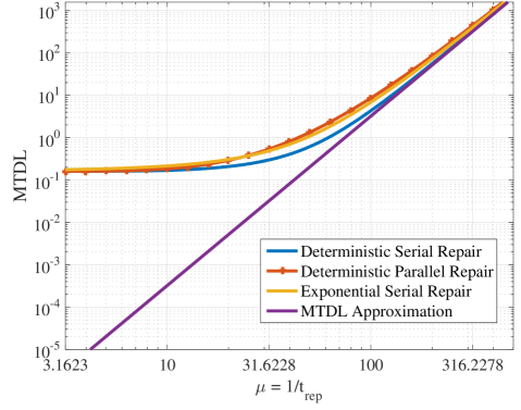
Refer to caption
Figure 1: Mean time to data loss for serial and parallel deterministic repair models, with comparison to the exponential serial repair and the approximation result.

We assume $n=10$ and $k=6$. We assume that the failue rate is $4$ per year. We plot the increase in mean time to data loss with decreasing time to repair in Figure 1. We note that for serial repair model, the mean time to data loss is lower for the deterministic repair model as compared to the serial exponential repair model. We further see that parallel deterministic repair has higher mean time to data loss as compared to serial deterministic repair. Finally, we note that the approximation result approximates all these three mean time to data loss expressions as the repair time becomes smaller.

V Conclusions

This paper gives Laplace Stieltjes transform of the data loss for the k-out-of-n distributed storage system with deterministic repair times. Two repair models, namely the serial and parallel repair are considered. We show that for failure rate much lower than the repair rate, mean time of data loss for the two models is the same unlike the case for exponential repair models.

References

  • [1] J. Kaplan, β€œMeeting the demand for data storage,” The McKinsey Quarterly, Nov 2008.
  • [2] L. Mearian, β€œWorld’s data will grow by 50X in next decade, IDC study predicts,” Computerworld, Jun 2011.
  • [3] P. M. Chen, E. K. Lee, G. A. Gibson, R. H. Katz and D. A. Patterson, β€œRAID: high-performance, reliable secondary storage,” Journal of the ACM Volume 26, Issue 2 (1994), p. 145-185.
  • [4] J. E. Angus, β€œOn computing MTBF for a k-out-of-n: G repairable system,” IEEE Transactions on Reliability Volume 37, Number 3 (1988), p. 312-313.
  • [5] M. S. Moustafa, β€œTime Dependent Availability of K-out-of-N:G Systems with Exponential Failures and General Repairs,” Economic Quality Control, vol. 18, no. 1, pp. 59-66, 2003.
  • [6] V. Aggarwal, C. Tian, V. A. Vaishampayan, and Y. R. Chen, β€œDistributed Data Storage Systems with Opportunistic Repair,” Proc. IEEE Infocom 2014.
  • [7] A. Campello and V. A. Vaishampayan, β€œReliability of Erasure Coded Systems: A Geometric Approach,” Proc. IEEE International Conference on BigData 2013, Santa Clara, CA, Oct. 2013.
  • [8] V. A. Vaishampayan and A. Campello, β€œReliability of Erasure Coded Storage Systems: A Combinatorial-Geometric Approach,” IEEE Transactions on Information Theory, vol. 61, no. 11, pp. 5795-5809, Nov. 2015.