Multilevel higher order Quasi-Monte Carlo
Bayesian Estimation
Abstract
We propose and analyze deterministic multilevel approximations for Bayesian inversion of operator equations with uncertain distributed parameters, subject to additive gaussian measurement data. The algorithms use a multilevel (ML) approach based on deterministic, higher order quasi-Monte Carlo (HoQMC) quadrature for approximating the high-dimensional expectations, which arise in the Bayesian estimators, and a Petrov-Galerkin (PG) method for approximating the solution to the underlying partial differential equation (PDE). This extends the previous single-level approach from [J. Dick, R. N. Gantner, Q. T. Le Gia and Ch. Schwab, Higher order Quasi-Monte Carlo integration for Bayesian Estimation. Report 2016-13, Seminar for Applied Mathematics, ETH Zürich (in review)].
Compared to the single-level approach, the present convergence analysis of the multilevel method requires stronger assumptions on holomorphy and regularity of the countably-parametric uncertainty-to-observation maps of the forward problem. As in the single-level case and in the affine-parametric case analyzed in [ J. Dick, F.Y. Kuo, Q. T. Le Gia and Ch. Schwab, Multi-level higher order QMC Galerkin discretization for affine parametric operator equations. Accepted for publication in SIAM J. Numer. Anal., 2016], we obtain sufficient conditions which allow us to achieve arbitrarily high, algebraic convergence rates in terms of work, which are independent of the dimension of the parameter space. The convergence rates are limited only by the spatial regularity of the forward problem, the discretization order achieved by the Petrov Galerkin discretization, and by the sparsity of the uncertainty parametrization.
We provide detailed numerical experiments for linear elliptic problems in two space dimensions, with parameters characterizing the uncertain input, confirming the theory and showing that the ML HoQMC algorithms outperform, in terms of error vs. computational work, both multilevel Monte Carlo (MLMC) methods and single-level (SL) HoQMC methods.
Key words: Higher order Quasi-Monte Carlo, parametric operator equations, infinite-dimensional quadrature, Bayesian inverse problems, Uncertainty Quantification, CBC construction, SPOD weights.
1 Introduction
In [9] we proposed and analyzed the convergence rates of higher order Quasi-Monte Carlo (HoQMC) approximations of conditional expectations which arise in Bayesian Inverse problems for partial differential equations (PDEs). We studied broad classes of parametric operator equations with distributed uncertain parametric input data. Typical examples are elliptic or parabolic partial differential equations with uncertain, spatially inhomogeneous coefficients, but also differential and integral equations in uncertain domains of definition. Upon suitable uncertainty parametrization, and with a suitable Bayesian prior measure placed on the, in general, infinite-dimensional parameter space, the task of numerical evaluation of Bayesian estimates for quantities of interest (QoI’s) becomes that of numerical computation of parametric, deterministic integrals over a high-dimensional parameter space. As an alternative to the Markov chain Monte Carlo (MCMC) method, in [22, 23] it was proposed to apply recently developed, dimension-adaptive Smolyak quadrature techniques to the evaluation of the corresponding integrals. In [9] we developed a convergence theory for HoQMC integration for the numerical evaluation of the corresponding integrals, based on our earlier work [6] on these methods in forward uncertainty quantification (UQ). In particular, we proved that dimension-independent convergence rates of order in terms of the number of approximate solves of the forward problem can be achieved by replacing Monte Carlo or MCMC sampling of the Bayesian posterior with judiciously chosen, deterministic HoQMC quadratures. The achievable, dimension-independent rate in the proposed algorithms is, in principle, as high as the sparsity of the forward map permits, and “embarrassingly parallel”: being QMC algorithms they access, unlike MCMC and sequential Monte Carlo (SMC) methods, the forward problem simultaneously and in parallel. The error analysis in [9] accounted for the quadrature error as well as for the errors incurred by a Petrov-Galerkin (PG) discretization and dimension truncation of the forward problem, but was performed for a single-level algorithm, i.e. the PG discretization of the forward model in all QMC quadrature points was based on the same subspace. As is well known in the context of Monte Carlo methods, multilevel strategies can lead to substantial gains in accuracy versus work. We refer to [13], and the references there, for a survey on multilevel Monte-Carlo methods. Multilevel discretizations for QMC integration were explored first for parametric, linear forward problems in [19, 16, 20] and, in the context of HoQMC for parametric operator equations, in [7]. For the use of multilevel strategies in the context of MCMC methods for Bayesian inverse problems we refer to [10, 17] and the references there. The purpose of the present paper is to extend the convergence analysis of the HoQMC, Petrov-Galerkin approach from [9] to a multilevel algorithm.
As in our single-level HoQMC PG error analysis of Bayesian inversion in [9], we adopt the abstract setting of Bayesian inverse problems in infinite-dimensional function spaces from [4], and the convergence analysis of PG discretizations of abstract, nonlinear parametric problems from [2, 21], as reviewed in [9]; throughout the present work, we adopt the notations and terminology from [9].
The principal contributions of the present work are as follows: we derive, for the possibly nonlinear, parametric operator equations with distributed, uncertain input considered in [9], multilevel extensions of high-order Petrov-Galerkin discretizations of the countably-parametric forward problem combined with HoQMC integration in the parameter domain. We provide a complete convergence analysis of the proposed algorithm, specifying, in particular, precise regularity and sparsity conditions on the forward response map which are sufficient to achieve a certain, dimension-independent convergence rate. Our analysis provides, in particular, information on the choice of algorithm parameters in applications: the convergence order of the PG discretization, also for functionals of the solution (not considered in [9]), the order of the interlaced polynomial lattice rule, the relation of HoQMC sample numbers and of truncation dimensions of the parameter space on the discretization level of the PG approximation of the forward problem. A major conclusion obtained with analytic continuation based error analysis from [8] is that identical algorithmic steering parameters are admissible in our ML HoQMC algorithm for both, forward and inverse UQ. With optimized HoQMC sample numbers, we also obtain asymptotic error vs. work bounds which indicate that the presently proposed algorithms outperform both, multilevel MC as well as the multilevel first order QMC algorithm considered in [19]; our analysis reveals that, analogous to sparse grid approximation, stronger regularity requirements on the parametric forward problem both in physical space and in parameter space are required.
In a suite of numerical experiments, we provide PDE examples in two space dimensions and with parameter spaces of dimension of several thousand where the presently proposed ML algorithms outperform all mentioned methods in terms of error vs. work, starting at relative errors as large as .
The structure of this paper is as follows. In Section 2, we present abstract, nonlinear parametric operator equations with uncertain input data, the parametrization of the uncertain input data and PG approximations of their parametric solutions. The setting is analogous to that from [9] and the presentation is thus synoptic, and analogous and with references to [9, Sections 2, 3]. In Section 3, we review the general theory of well-posed Bayesian inverse problems in function spaces, from [4]. Again, the material is analogous to what we used in [9]; however, the error analysis of the ML HoQMC method, being a form of sparse grid approximation, requires the analog of mixed regularity, which we develop. Section 4 contains the core new mathematical results of the present paper: several multilevel computable Bayesian estimators and their error analysis. In particular it contains the error vs. work analysis of the combined ML HoQMC Petrov-Galerkin algorithms. Section 5 presents specific examples of parametric forward problems, and verifies that they satisfy all hypotheses of our foregoing error analysis; specifically, we consider linear, affine-parametric diffusion problems in two space dimensions, in primal variational formulation with space of continuous, piecewise linear functions on regular triangulations. Section 6 contains numerical tests of the proposed estimators for forward and inverse UQ for the PDE problems considered in Section 5. The numerical results are in agreement with the theory.
2 Forward UQ for parametric operator equations
We review the notation and mathematical setting of forward and inverse UQ for a class of smooth, possibly nonlinear, parametric operator equations, for which we developed the error analysis of the single-level algorithm in [9]. We develop here the error analysis for the multilevel extension of the algorithms in [9] for a general class of forward problems given by smooth, nonlinear operator equations with input data from a separable Banach space . Upon uncertainty parametrization with an unconditional basis of such as, for example, the Karhunen-Loève basis, both forward and (Bayesian) inverse problems become countably parametric, deterministic operator equations. The problems of forward and inverse UQ are reformulated as countably-parametric integration problems. In the present work, we focus on the latter and analyze the use of deterministic, higher order Quasi Monte-Carlo integration methods, from [6, 7, 8] and the references there, in multilevel algorithms for Bayesian estimation in partial differential equations with uncertain input.
2.1 Uncertainty parametrization
As in [9], we parametrize the distributed uncertain input data . To this end, is assumed to be a separable, infinite-dimensional Banach space with norm , which has an unconditional basis : . Let be fixed. Any has the representation
| (2.1) |
where means convergence in the norm of . The Karhunen-Loève expansions (see, e.g., [27, 26, 28, 4]) are examples of representations (2.1). We remark that the representation (2.1) is not unique: rescaling and will not change .
Assume that a smoothness scale , with , and a is being given as part of the problem specification. We restrict the uncertain inputs to sets with “higher regularity” in order to obtain convergence rate estimates for the discretization of the forward problem. Note that often corresponds to stronger decay of the in (2.1). We assume that the are scaled such that
| (2.2) |
We define the set by
| (2.3) |
where . Further we define the sequences by for . If , we write and . From (2.2) we have for . We also assume that the are enumerated so that
| (2.4) |
With a given unconditional basis , realizations of correspond to pairs , where is the nominal value of uncertain data and is the coordinate vector that determines the unique representation (2.1).
2.2 Operator equations with uncertain input
We consider the abstract forward problem:
| (2.5) |
Here, and are real, separable Banach spaces and is the residual of a forward operator.
A solution of (2.5) is called regular at , for a given , if and only if the map is Fréchet differentiable with respect to at and if the differential is an isomorphism between and . We assume the map admits a family of regular solutions locally, in an open neighborhood of the nominal parameter instance , so that the operator equations involving are well-posed. A particular structural assumption on is the representation
| (2.6) |
with Frechet differentiable maps and . The set is called regular branch of solutions of (2.5) (in the sense of [2]) if
| (2.7) |
The regular branch of solutions (2.7) is called nonsingular if, in addition, the differential
| (2.8) |
Conditions for well-posedness of (2.5) are stated in [8, Proposition 2.1]: for regular branches of nonsingular solutions given by (2.5) - (2.8), the nonsingularity of the differential implies the inf-sup conditions. Under the inf-sup conditions, for every instance , there exists a unique, isolated solution of (2.5), which is uniformly bounded in the sense that there exists a constant such that
| (2.9) |
The set is called a regular branch of nonsingular solutions.
At every point of the regular branch , if the nonlinear functional is Fréchet differentiable with respect to and Fréchet differentiable with respect to , then the mapping relating to within the branch of nonsingular solutions is locally Lipschitz on :
| (2.10) |
In what follows, we consider the abstract setting (2.5) with the assumption that the mapping is uniformly continuously differentiable with boundedly invertible differential in a product of neighborhoods , where denotes the ball with radius , of sufficiently small radius . Then is the corresponding unique, isolated solution of (2.5) at the nominal uncertain input . This turns (2.5) into an equivalent, deterministic, countably parametric operator equation: given , find such that
| (2.11) |
We refer to [9, Remark. 2.1] for further discussion. Under (2.9) and (2.10), the operator equation (2.5) will admit a unique solution for every . This solution is, due to (2.9), uniformly bounded,
| (2.12) |
and due to (2.10), it depends Lipschitz continuously on the parameter sequence : there exists a Lipschitz constant such that
| (2.13) |
The Lipschitz constant in (2.13) is generally different from the constant in (2.10), as it depends on and on the basis . Unless explicitly stated otherwise, throughout what follows, we shall identify with the solution of (2.5) at the nominal input .
Note that implies that and , with corresponding subspaces and with extra regularity from suitable scales. If , we write , , etc..
2.3 Dimension truncation
Dimension truncation is equivalent to setting for , for a given , in (2.1). The truncated uncertain datum is denoted by . We denote by the solution of the corresponding parametric weak problem (2.11). For , define . Then unique solvability of (2.11) implies . Consider the -term truncated parametric problem: given ,
| (2.14) |
As shown in [9, Prop. 2.2], [18, Thm. 5.1], under Assumption (2.2), and under the uniform regularity shift in (2.18) ahead, for every , for every and for every the parametric solution of the truncated parametric weak problem (2.11) with replaced by satisfies, with as defined in (2.2),
| (2.15) |
Moreover, for every , there exists such that
| (2.16) |
where
for some constant independent of .
2.4 Petrov-Galerkin discretization
In [14, Chap. IV.3] and in [21], a convergence rate analysis of Petrov-Galerkin discretizations of regular branches of solutions for smooth, nonlinear forward problems (2.5) was developed. This setting was adopted in [9] and is also the basis for the presently considered multi-level extension of the single-level version of the present work [9]. As in [25, 6], we assume that we are given two sequences and of finite dimensional subspaces which are dense in and in , respectively. We assume the following regularity properties and approximation properties:
uniform parametric regularity property (UPR): there are scales and of function spaces such that and for any and analogously for , such that there holds the uniform regularity shift: for as in (2.6), for every , , the parametric solutions and , where is the conjugate operator of , satisfy regularity resp. adjoint regularity shifts which are uniform w.r. to , i.e.
| (2.18) |
We also assume approximation properties: for and for holds
| (2.19) |
Assume that the subspace range and are stable in the following sense: there is and a discretization parameter such that for every , the discrete inf-sup conditions hold uniformly (with respect to )
| (2.20) | ||||
| (2.21) |
Then, for every , the solutions of the Petrov-Galerkin approximation problem:
| (2.22) |
are uniquely defined and converge quasioptimally: there is a positive constant such that for all
| (2.23) |
If for all and if (2.19) holds, then for every
| (2.24) |
Moreover, for sufficiently large truncation dimension , for given the solutions of the following truncated Galerkin problems
| (2.25) |
admit unique solutions which converge quasioptimally to as , i.e. (2.23) and (2.24) hold with in place of , with the same constants and independent of and of .
3 Bayesian inverse UQ and HoQMC approximation
In this section, the abstract (possibly nonlinear) operator equation (2.5) is considered again. The system’s forcing is allowed to depend on the uncertain input and the uncertain operator is boundedly invertible, for the uncertain input , sufficiently close to a nominal instance of the uncertain input data . We define the forward response map, which maps a given uncertain input and a given forcing in (2.6) to the response in (2.5) by
In the general case (2.5), we omit and denote the dependence of the forward solution on the uncertain input as . A bounded linear observation operator on the space of observed system responses in is given and denoted by . Throughout the remainder of this paper, we assume that with , then . The space is equipped with the Euclidean norm, denoted by .
We assume the following form of observed data, composed of the observed system response and the additive noise
| (3.1) |
The additive observation noise process is assumed to be Gaussian, i.e. a random vector with a positive definite covariance on .
The uncertainty-to-observation map then reads , so that
| (3.2) |
When varies randomly, varies in , the space of random vectors taking values in which are square integrable with respect to the Gaussian measure with covariance matrix . Bayes’ formula from [28, 4] implies, for the -variate parametric problems, existence of a density of the Bayesian posterior with respect to the prior. Its negative log-likelihood equals the observation noise covariance-weighted, least squares functional (“potential”) by
| (3.3) |
3.1 Well-posedness and approximation
In deterministic problems, the data-to-solution maps is often ill-posed. In the presently considered setting, for a positive definite covariance , the expectations (3.19) are Lipschitz continuous with respect to the data , provided that the potential in (3.3) is locally Lipschitz with respect to the data .
Assumption 1.
[4, Assumption 4.2] Let denote a subset of admissible uncertain input data, and assume that is Lipschitz on bounded sets.
Assume also that there exist functions , , (depending on ) which are monotone, non-decreasing separately in each argument, and with strictly positive, such that for all , and for all
| (3.4) |
and
| (3.5) |
In [4, Thm. 4.3], a version of Bayes’ rule in function spaces is considered and the following result is shown.
Proposition 3.1.
Let Assumption 1 hold. Assume further that and that for some bounded set . Assume additionally that, for every fixed ,
Then
(i) for -a.e. data ,
(ii) the conditional distribution of ( given ) exists and is denoted by . It is absolutely continuous with respect to and there holds
| (3.6) |
The Bayesian posterior admits a derivative w.r. to the prior with a bounded density w.r.t. the prior , which is given by (3.6).
We remark that in the present context, (3.5) follows from (3.3); for convenient reference, we include (3.5) in Assumption 1. Under Assumption 1, the expectation (3.19) depends Lipschitz continuously on the data (see, e.g., [4, Sec. 4.1] for a proof):
| (3.7) |
For , the Bayesian posterior with respect to the approximate potential obtained from dimension truncation at dimension and PG discretization (2.25), with degrees of freedom, is well-defined. The multi-level convergence analysis requires bounds on the approximation errors in the response due to discretization and approximate numerical solution of the discretized problems) on the Bayesian estimate (3.19). To bound the errors of the Bayesian expectations (3.19) as in [9], we work under
Assumption 2.
[4, Assumption 4.7] Let denote a subset of admissible uncertain input data, assume that , and let the Bayesian potential be Lipschitz on bounded sets. Assume also that there exist functions , , independent of the number of degrees of freedom in the PG discretization of the forward problem, where the functions are monotonically non-decreasing separately in each argument, and with strictly positive, such that for all and for all ,
| (3.8) |
and there is a positive, monotonically decreasing such that as , monotonically and uniformly w.r.t. (resp. w.r.t. ) and such that
| (3.9) |
Proposition 3.2.
A proof of Proposition 3.2 can be found in [4, Thm. 4.9, Rem. 4.10]. The consistency condition (3.9) in either of these cases follows from [9, Prop. 3.2]. Assume we are given a sequence of approximations to the forward response such that, with the parametrization (2.1),
| (3.11) |
with a consistency error bound as in Assumption 2. Denote by the corresponding (Petrov-Galerkin) approximations of the parametric forward maps. Then it was shown in [9, Prop. 3.2] that the approximate Bayesian potential
| (3.12) |
where , satisfies (3.9). In the ensuing error analysis of the combined HoQMC, PG approximation, in (3.12) will denote the Petrov-Galerkin discretization (2.25) in Section 2.4, based on -dimensional truncation of the parameter space, and on finite dimensional subspaces with many degrees of freedom. Typically, for subspaces of piecewise polynomial functions obtained by isotropic mesh refinement in a bounded, physical domain , ; in sparse grid discretizations in (not considered in detail here, but covered by the present theory), . In that case, and are function spaces of mixed partial derivatives.
In applying QMC to Bayesian estimation, we shall be concerned with integration of parametric integrand functions with respect to a probability measure on the set of all parameters characterizing the uncertain input data. Typically, will denote a Bayesian prior on . Since is a cartesian product of intervals, we assume that is a product probability measure, i.e. .
3.2 Parametric Bayesian posterior
As in [22, 23, 9] and in Section 2.1, we adopt a product probability space
| (3.13) |
We assume that the prior on the uncertain input , parametrized in the form (2.1), satisfies . We also assume the prior measure being uniform, and the sequences in (2.1) taking values in the parameter domain . With as in (3.13), the uncertainty-to-observation map reads
| (3.14) |
In order to apply our QMC quadrature, we need a parametric version of Bayes’ Theorem, as stated in Prop. 3.1, in terms of the uncertainty parametrization (2.1). We view as the unit ball in , the Banach space of bounded sequences taking values in .
Proposition 3.3.
Assume that is bounded and continuous. Then , the distribution of given data , is absolutely continuous with respect to , i.e. there exists a parametric density such that for every
| (3.15) |
with the posterior density given by
| (3.16) |
Here the Bayesian potential is as in (3.3) and
| (3.17) |
Bayesian estimation aims at a “most likely” value of the Quantity of Interest (QoI) (in a Banach space ), conditional on given (noisy) observation data . For example, (with ) will result in a “most likely” (as expectation under the posterior, given data ) system response. Based on Prop. 3.3 we associate with the QoI the deterministic, infinite-dimensional, parametric map
| (3.18) |
With the density in (3.18), the Bayesian estimate of the QoI , given noisy data , takes the form
| (3.19) |
3.3 Higher order QMC integration
In general, the integrals and in (3.19) cannot be evaluated exactly. Hence we propose to approximate these integrals by a HoQMC quadrature rule. In the following, we assume the prior density to be the uniform density. Supposing is a collection of QMC points, we define the QMC estimate of the integral of a function with respect to the uniform measure by the following equal weight quadrature rule in dimensions,
| (3.20) |
We shall analyze, in particular, being deterministic, interlaced higher order polynomial lattice rules as introduced in [5] and as considered for affine-parametric operator equations in [7].
To generate a polynomial lattice rule with points (where is a given prime number, is a given positive integer), we need a generating vector of polynomials where each is a polynomial with degree with its coefficients taken from a finite field .
For each integer , we associate with the polynomial
where is the -adic expansion of , that is . We also need a map which maps elements in to the interval , defined for any integer by
Let be an irreducible polynomial with degree . The classical polynomial lattice rule associated with and the generating vector is comprised of the quadrature points
Classical polynomial lattice rules give almost first order of convergence for integrands of bounded variation. To obtain higher order of convergence, an interlacing procedure described as follows is needed. The digit interlacing function with digit interlacing factor is given by
| (3.21) |
where for . For vectors, we set
| (3.22) |
Then, an interlaced polynomial lattice rule of order with points in dimensions is a QMC rule using as quadrature points, for some given modulus and generating vector .
3.4 Holomorphic parameter dependence
In the QMC quadrature error analysis, for each parameter , for , we assume the parametric family of solutions admits a holomorphic extension into the complex domain and these extensions must satisfy some uniform bounds. We recall from [15, 3] the notion of -holomorphy of parametric solutions introduced to this end. In the remainder of Section 3.4 all spaces , , and will be assumed to be Banach spaces over .
Definition 3.1.
(-holomorphy) Let and be given. For a positive sequence , a parametric mapping satisfies the -holomorphy assumption if and only if all of the following conditions are satisfied:
-
1.
The map from to , for each , is uniformly bounded with respect to the parameter sequence , i.e. there is a bound such that
(3.23) -
2.
For any -admissible sequence , for sufficiently small , the parametric solution admits a continuous extension to the complex domain with respect to each variable that is holomorphic in a cylindrical set of the form where, for every , is an open set . Recalling that, the sequence is -admissible if
(3.24) -
3.
For any poly-radius satisfying (3.24), there are open sets
such that the parametric map admits a continuous extension to which is bounded: there holds
(3.25) where the bounds depend on , but are independent of .
Evidently, -holomorphy depends on the choice of . For derivative estimates in the HoQMC error bounds in [6, 18], we use as in [8] a specific family of continuation domains: for , define
| (3.26) |
Then, once more, for a poly-radius satisfying (3.24), we denote by the corresponding cylindrical set . We refer to [15, 3] and the references there for further examples of parametric forward problems whose solutions admit -holomorphic extensions.
3.5 HoQMC convergence for -holomorphic integrands
To obtain QMC error bounds, we quantify the dependence of the parametric solution of (2.5) on the parameter sequence . As shown in [18], bounds on the growth of the partial derivatives of with respect to imply convergence rates for higher order QMC quadratures.
We are interested in integrand functions being compositions of with PG approximation of the dimension-truncated, parametric and -holomorphic, operator equation (2.5). For every , is -holomorphic uniformly w.r.t. (see Section 2.3). Based on [6, Sec. 3] and [8, Prop. 4.1], the following result provides rates of convergence of QMC quadratures.
Proposition 3.4.
Assume given a parameter space dimension and integration points for integer and for a prime number . Let be a sequence of positive numbers, and denote by its truncation after terms. Assume that for some , i.e. that
| (3.27) |
Define, for as in (3.27), the digit interlacing parameter
| (3.28) |
Consider parametric integrand functions in a separable Hilbert space which are -holomorphic (cp. Definition 3.1).
Then, for every , one can construct an interlaced polynomial lattice rule of order with points using a fast component-by-component algorithm, in at most operations, plus update cost, plus memory cost, and with the error bound
| (3.29) |
Here is independent of and , and the expression denotes the (likewise independent of and of ) maximum of the modulus for the integrand function over for every -admissible poly-radius (i.e., satisfying (3.24)) :
| (3.30) |
Proof.
The Hilbert space being isomorphic to , for every the norm can be written as
where denotes the inner product. By separability of , the Bochner-integral and the QMC rules are well-defined also for measurable integrand functions taking values in . For integrand functions being a -holomorphic map taking values in , for every the mapping is a -holomorphic map with values in . Therefore, the complex variable HoQMC error bounds obtained in [8, Prop. 4.1] apply for this integrand: there exists a constant which is independent of the parametric integrand such that for every holds the HoQMC error bound
| (3.31) |
Here, for every fixed and any -admissible poly-radius ,
The linearity of and of imply that for every holds
We may therefore estimate with (3.31)
∎
4 Multilevel HoQMC Bayesian estimators
4.1 Multilevel discretization of the forward problem
Multilevel Bayesian estimators are based on a hierarchy of discretizations of the forward problem (2.5). Below we design increasing sequences and of truncation dimensions and QMC sample numbers at discretization level , and a decreasing sequence of discretization parameters. With this latter sequence, we associate nested, dense sequences and of discretization spaces of increasing, finite dimension . We refer to the pairs as PG discretization parameters, and also set and . We denote by the dimensionally truncated, PG approximated parametric forward solution in (2.25). The consistency error bounds for approximations of the Bayesian posterior, (3.10), imply that the Bayesian estimates incur an error which is bounded by the error of the PG discretization in the forward problem, provided posterior expectations are evaluated exactly.
The potential based on the solution of (2.5) on discretization level is denoted as , and is given in (3.12). The corresponding approximations to the posterior density from (3.16) are then
| (4.1) |
The exact normalization constant for the forward model at discretization level is then
| (4.2) |
Note that , as defined in (4.1), includes also a dimension truncation to dimension .
In our ensuing error analysis of the Bayesian estimators, we shall use the bound (3.29) for various choices of ; in particular, with both with , and with denoting the QoI.
4.2 Multilevel Bayesian estimators
We now describe two multilevel estimators, the ratio estimator proposed in [22, 23] and the splitting estimator, inspired by [1]. The ratio estimator is based on expanding the two integrals and separately, and the splitting estimator is based on a joint telescopic expansion of . In conjunction with deterministic higher order QMC integration (3.20), either estimator will result in deterministic algorithms for Bayesian estimation of PDEs with distributed, uncertain input with high convergence rates which are independent of the dimension of the parameter space.
4.2.1 Multilevel ratio estimator
It was proposed in [22, 23] to numerically evaluate the Bayesian estimates (3.19) by “direct integration”, i.e. by applying a deterministic quadrature rule to the (formally) infinite-dimensional, iterated integrals in the normalization constant and the QoI . In [22, 23], dimension adaptive Smolyak quadrature was used to compute . Here, as in [9], we evaluate by approximating the integrals and by HoQMC integration. In [9] we used single-level estimators for numerator and denominator; here, we develop a MLHoQMC estimator. To derive it, we write, using the telescopic sum identity and denoting integration with respect to the prior by ,
| (4.4) | ||||
and the corresponding ML approximation of the normalization constant ,
| (4.5) | ||||
We approximate the integrals in (4.4) and (4.5) on discretization level with a higher order QMC rule based on points, resulting in the Multilevel Higher Order QMC estimators and , respectively. Note that both estimators (for and ) can be computed simultaneously, without having to reevaluate the forward model. The multilevel ratio estimator is thus given by
| (4.6) |
with the individual multilevel approximations (omitting the variables ) given by the multilevel algorithm of [19, 7], i.e.
| (4.7) | ||||
| (4.8) |
4.2.2 Multilevel splitting estimator
We consider approximations of the form (4.3) on each discretization level and write
| (4.9) |
We now apply QMC quadrature to the integrals in , for each , where we approximate all terms on the same discretization level (i.e. all terms inside the parenthesis) by a QMC rule with points, resulting in the Multilevel High Order QMC estimator . Denoting by and the HoQMC approximations of and on quadrature level , the multilevel QMC splitting estimator reads
| (4.10) |
Thus, on discretization level we must compute the two approximations and , and for each discretization level we evaluate four approximations
| (4.11) |
Since all four approximations involve the same QMC quadrature points, the additional quadratures do not require extra solutions of the forward model on level or . Therefore, they do not increase the work significantly, assuming the cost of representing elements of in an implementation are negligible. In the case where different truncation dimensions are used, the “quadrature point” on level can be truncated at dimension : on level .
Remark 4.1.
The differences in the formula (4.9) can be written as the following expression (bearing in mind that index signifies implied dimension truncation to dimension )
| (4.12) |
see (4.3). This form corresponds to the splitting which is customary in MCMC and SMC methods, see, e.g. [1] and the references there. We expect the application of QMC quadratures in finite arithmetic to the integrand function in (4.12) to be advantageous for small observation covariance . The integrand function of (4.12) is, upon suitable (-dependent) rescaling of coordinates as in [24, Theorem 4.1], -holomorphic uniformly with respect to .
4.3 Error analysis
Each of the proposed computable estimators (4.6), (4.10) is based on approximating posterior expectations of PG discretizations and dimensionally truncated forward models by HoQMC integration. The ensuing error analysis is based on the dimension independent error bounds for these quadratures which we developed in [6, 7]. These bounds are based on estimates of higher order derivatives of the integrand functions with respect to the integration variables. In [8, Section 3], we developed estimates for these derivatives based on analytic continuation of integrand functions into the complex domain and Cauchy’s integral formula; this is feasible for holomorphic forward problems considered in [3], and for general, holomorphic potentials . As is by now well-known, and in contrast to our single-level QMC error analysis for the quotient estimator in [9], multilevel QMC error estimates involve bounding quadrature errors of PG forward problem discretization errors. To use the higher order QMC error bounds of [8] in the present multilevel context therefore requires bounds on the dimension truncation and PG discretization errors of analytic continuations of the integrand functions. These bounds are to hold uniformly with respect to the truncation dimension . The present, analytic continuation approach should be contrasted with the “real-variable” approach used in the error analysis of QMC integration in [7], which is based on bootstrapping arguments and induction.
4.3.1 Holomorphy assumptions on the PG approximation
To ensure holomorphy of countably parametric families of integrand functions in the Bayesian estimators (4.6), (4.10), as required by the QMC error bounds stated in Proposition 3.4, we impose corresponding holomorphy assumptions on the parametric forward problem (2.11) as well as on its PG discretization (2.25). We formalize these conditions (which are versions of the uniform parametric regularity UPR and the parametric stability) in the following:
(i) Holomorphic continuation of the parametric forward problem in : there is a -holomorphic extension of the parametric forward problem (2.14) such that, for any truncation dimension , and for every , the extended problem
| (4.13) |
admits a unique, parametric solution which is -holomorphic.
(ii) PGStabC Stability and Quasioptimality of the PG discretization for the complex parametric extension: for every , and for every the Galerkin approximations:
| (4.14) |
are uniquely defined and converge quasioptimally: there exists a constant such that for all , with a -admissible poly-radius ,
| (4.15) |
We remark that and PGStabC imply, via the approximation property (2.19), the convergence rate in for the Galerkin solution , with implied constant independent of the truncation dimension .
(iii) Aubin-Nitsche argument for the PG discretization of the complex parametric extension: There exists a constant such that for every there holds a superconvergence estimate: for every which is -admissible for sufficiently small ,
| (4.16) |
Examples with valid conditions (i) - (iii) will be presented in the numerical experiments Section 5 ahead; the hypotheses will be verified in particular for affine-parametric operator equations in Section 5.1.
4.3.2 Error bounds for the multilevel ratio estimator
Numerator and denominator of the estimator (4.6) are approximated separately by MLHoQMC estimators, (4.7), (4.8). We first analyze the error of these approximations, thereby also generalizing the single-level results in [8]. Throughout, we assume that in all densities which occur in the integrals (3.17) - (3.19) the parametric forward problems are dimension-truncated to finite parameter dimensions for discretization levels , which we assume to be strictly increasing (the ensuing error analysis remains valid with obvious modifications, if several or all truncation dimensions are equal) i.e.
Throughout the error analysis, we assume and is as in (2.16).
Theorem 4.1.
Assume that , for some and that, in addition, there exists such that , uniformly with respect to . Assume also , hold for some .
Then, for every , with as in (2.16),
| (4.17) |
Proof.
Since , we estimate
| (4.18) |
The first term is the exact posterior expectation on the approximate forward model, i.e. a pure discretization error. It can be estimated using Proposition 3.2 and the approximation property (2.19) with property . There exists a constant which is independent of and of such that
| (4.19) |
To bound term in (4.18), we write it as telescoping sum
| (4.20) |
The first term in (4.20) is a pure QMC integration error, on the coarsest level PG discretization; it can be estimated with (3.29). The remaining terms are QMC quadrature errors of dimension truncation and Petrov-Galerkin errors. A typical term reads
| (4.21) |
We rewrite a generic term in the telescoping sum (4.20) as (parameter not indicated)
Here, we used the linearity of the QoI .
To apply the QMC quadrature error bound (3.29) with , we need to estimate (cp. (3.30)) for with being -admissible
| (4.22) |
We estimate each of the two differences in essentially the same way. Consider . Then
The first two terms are PG discretization errors for the complex-parametric extension of the operator equation. Property (holomorphic continuability of the parametric forward problem) implies the well-posedness of the complex-parametric problem, and assumption PGStabC (stability of the PG discretization in the complex-parametric problem) implies that the PG discretization errors can be bounded as
| (4.23) |
provided that is -admissible. The third term is a dimension truncation error. It vanishes if , and by the stability of the PG discretization is bounded for any by
| (4.24) |
As the modulus of the posterior density, , is uniformly bounded w.r.t. and w.r.t. , for any -admissible , the first term in the bound (4.22) can be estimated for by an absolute multiple of
| (4.25) |
For a fixed -admissible poly-radius , and for any we estimate the second term in (4.22) by
| (4.26) |
Here, the latter supremum is bounded uniformly w.r.t. , due to condition PGStabC: the uniform stability of the PG discretization for the complex-parametric problem implies also the existence of a bound , independent of the discretization level such that
We focus on the first supremum in (4.26).
| (4.27) |
We deal with three errors in the posterior density, which arise due to different approximations in the forward maps.
To reduce the error in the posterior density to an error bound in the corresponding potentials , we recall definition (3.3) (applied with transposition to the complex-parametric forward map) and write
, where the complex integral is along a straight line in connecting and .
The difference in the Bayesian potentials due to the PG discretization (at equal truncation dimension ) of the forward problem is estimated using (a complex-parametric extension of) (3.11) again in terms of the PG forward discretization error.
We obtain for every which is -admissible the bound
The third term in (4.27) is bounded in the same way in terms of the error (4.24), resulting also for (4.26) in the upper bound (4.25). Collecting all bounds, we have shown that for any poly-radius which is -admissible, there exists a constant such that for any and for all
Combining this with (4.19), we obtain from (4.18) the error estimate
| (4.28) |
By choosing , and , the bound (4.28) applies also for the approximation of .
4.3.3 Error bounds for the multilevel splitting estimator
Theorem 4.2.
Assume that , for some and that, in addition, there exists such that , uniformly with respect to . Assume , hold for some . Then, for every , with as in (2.16),
| (4.30) |
Proof.
For given sequences , of truncation dimensions and numbers of QMC points, and for given by (4.3), we estimate
To bound the first term, we use Proposition 3.2 (see (3.10)) and the approximation property (2.19) and the dimension truncation estimate (2.15) with the discretization parameters ,
To bound the second term, we write, after subtracting (4.9) and (4.10)
We rewrite the difference between the -th term in the sum over in (4.9) and (4.10) as
We rewrite upon adding and subtracting the term as
| (4.31) |
For the first term in the right hand side of (4.31), we observe that
Using the estimates of (4.21) in the previous section we obtain
where is independent of and of . For the second term in (4.31), we have
and
Adding and subtracting the term , we may rewrite as
| (4.32) |
Using Proposition 3.4 and the fact that is uniformly bounded with respect to and , we have
| (4.33) |
If , uniformly with respect to , for some , then there exists (depending on , but independent of or ) such that
| (4.34) |
Using similar techniques as in the estimates of (4.27),
Thus, for any sequence or , the -norm of the first term of (4.32) is bounded by , for any .
For the second term of (4.32), adding and subtracting the same term
| (4.35) | ||||
| (4.36) |
We bound (4.35) by similar techniques as in the estimates (4.21) to arrive at the bound
For the remaining term (4.36), we rewrite the first factor as
| (4.37) |
Using similar estimates as in (4.27), we conclude that there exists independent of and of such that
| (4.38) |
All are bounded above and below away from zero for , and the first factor of (4.36) is bounded by the RHS of (4.38). The second factor of (4.36) is estimated by
Combining all estimates for (4.35) and (4.36), we conclude that there exists a constant such that, for every , and for all sequences , and holds
Therefore, both and in (4.31), (4.32) are bounded by (with constant independent of , or ). Summing the preceding estimates over all discretization levels, we arrive at the error bound (4.30) for the splitting estimator. ∎
4.3.4 Selection of truncation dimensions and sample numbers
We assume in the following that assumption holds for some , and define . The error analysis of the computable MLHoQMC Bayesian estimators in Sections 4.3.2 and 4.3.3 lead to error bounds (4.29) and (4.30), respectively, which are of the generic form
| (4.39) |
with , and which is analogous to the bounds proved for MLHoQMC algorithms for forward UQ in [7] under with some . In (4.39), the maximal rate in is obtained for the choice , implying for the digit interlacing factor. Moreover, to obtain the maximal rate for we choose as small as possible, which yields since .
Choice of truncation dimension.
In a first step, we balance the dimension truncation error on level with the discretization error on level , and similarly for the increment levels . We assume in the following the behavior for and . For the terms on level , we have , which motivates the choice . Using (cp. [7, Eqn. (1.12)]), we have for the increments , which leads to . Since the discretization error on mesh level limits the accuracy of the entire computation, increasing the parameter space dimension beyond is unnecessary; we therefore choose the truncation dimensions
| (4.40) |
Error and work models.
We now use (any sequence with uniformly bounded ratios would be admissible in the error analysis) and the preceding equilibration of the dimension truncation and FEM discretization errors to obtain an expression for the total error. We replace by , since for holds for ,
| (4.41) |
The total work (cost) is given by
| (4.42) |
Optimization of the number of samples.
We now seek to minimize the error bound (4.41) subject to a given, fixed work budget for (4.42). A minimum can be found using a Lagrange multiplier . To ease the ensuing calculations, we assume all constants in the asymptotic error bounds equal . Then, we consider the Lagrangian
Now, we consider the necessary condition that for all . For now, we consider to be a free parameter (to be determined), and use this to find an expression for the multiplier from the following condition:
| (4.43) |
Note that the assumption can lead to a large increase in the sample numbers in the MC case, if it is not fulfilled. In the numerical experiments ahead, this assumption does not hold, since we use with .
Inserting (4.43) into the remaining conditions for yields
Inserting this expression for into (4.41), we set and write the total error as
and determine by equilibrating the two contributions , which yields
Since we consider interlaced polynomial lattice rules with points, we choose for as
| (4.44) |
4.3.5 Multilevel Monte Carlo (MLMC) sampling
An alternative to QMC evaluation of the ratio and splitting estimators is to approximate the prior expectations and by MC sampling. In MC, the convergence rate is (in mean square, however) in terms of the number of MC samples, independent of the summability exponents . The MLMC variant of MC appears as a particular case of the above algorithms; a general optimization of the level-dependent sample numbers yields the same truncation dimensions as in (4.40) above and the following choice of number of samples. Note, however, that in MC sampling we do not simply set , since the truncation dimensions still depend on the value of the summability exponent . We obtain with and the sample numbers
| (4.45) |
5 Model forward problems
We present examples of forward problems and discretizations which verify the abstract hypotheses of the foregoing error analysis. In Section 5.1 we verify that properties , and of Section 4.3.1 hold for rather general classes of linear, affine-parametric operator equations. Next, in Section 5.2, we consider a concrete linear elliptic problem in two space dimensions with a particular, explicit selection of the uncertainty parametrization (2.1). We remark that analogous hypotheses are valid for a host of more general problems with high-dimensional uncertainty parametrization; we mention only parametric systems of nonlinear ODEs [15], and PDE problems with domain uncertainty.
5.1 Affine-parametric linear operator equations
We verify the abstract hypotheses of the QMC-PG error analysis in Section 4.3.1 for the model problem (5.8) below; in doing so, rather than considering the particular problem (5.8), we consider the more general linear, affine parametric operator equations as considered in [25].
For a regularity parameter , let be a sequence of bounded, linear operators which satisfy the following hypotheses.
is boundedly invertible, i.e. .
For , the sequences of norms satisfy for summability exponents .
There holds .
Under H1 - H3, we consider for parameter sequences , and for the linear, affine-parametric operators given by
| (5.1) |
Evidently, then, the differential of the residual map equals , and the (uniform w.r.t. ) bounded invertibility of implies a uniform (w.r.t. ) inf-sup condition for . Hypotheses - imply, with a Neumann series argument, properties and in Section 4.3.1 for the affine-parametric family (5.1) of linear operators. Specifically, for every and for every holds in (with for )
| (5.2) |
Denoting by and “complexifications” of the function spaces, the affine-parametric operator family in (5.1) extends to the polydisc , and the Neumann series inversion formula (5.2) remains valid for . The extended family being affine-parametric is holomorphic with respect to each variable and, by , is also boundedly invertible in for all , provided the poly-radius is -admissible, i.e. provided that (3.24) holds for some . Since the mapping is analytic at any , (5.2) defines a parametric solution family , which, for and some , is -holomorphic with holomorphy domains in Definition 3.1 being the polydiscs . For every -admissible there holds the holomorphic continuability of the parametric solutions for some , so that
| (5.3) |
As for every , , Proposition 3.4 is applicable to for any QoI .
The Neumann series argument used to verify (5.3) also implies condition PGStabC (Stability and Quasioptimality of PG for the complex parametric extension). To see this, we assume at hand a nested sequence of (dense in ) finite-dimensional PG trial- and test function spaces, which satisfy the nominal inf-sup condition: there exists such that
| (5.4) |
With (5.4), assumption implies PGStabC, i.e. Stability and Quasioptimality of the PG discretizations for the complex parametric extension to for any -admissible polyradius : for such holds
which implies with (5.4) and with that
| (5.5) |
Assume that is -admissible for the sequence given by for , and for sufficiently small . Hypothesis , i.e. that is an isomorphism, implies . By H2 and H3, implies with H1 that . The -admissibility of and with imply
which implies in (5.5) the uniform (w.r.t. ) parametric discrete inf-sup conditions
| (5.6) |
with independent of . The uniform parametric inf-sup conditions (5.6) imply uniform w.r.t. stability of the PG discretization and the existence, uniqueness and the quasioptimality of the complex-parametric PG solution , for every with -admissible . It also implies the (uniform w.r.t. the discretization level ) -holomorphy of the PG solutions . The quasioptimality and the uniform parametric regularity (5.3) imply, with the approximation property (2.19), the (uniform w.r.t. ) asymptotic error bounds
| (5.7) |
where the constant is independent of , and of , but depends on and in the -admissibility of the poly-radius . Choosing , (5.7) implies (4.23). For the linear, affine-parametric operators (5.1), property for some was shown in [7], for the affine-parametric, linear operator family (5.1).
5.2 Affine-parametric linear test problem
We test the proposed ML algorithms for a model parametric, linear diffusion problem which was already considered in [7].
For a parameter , in the bounded spatial domain , we consider the second order, linear and affine-parametric elliptic PDE
| (5.8) |
This is a particular (linear) forward problem (2.5). The usual (symmetric) primal variational formulation of (5.8) is based on . In the particular case that , we parametrize the uncertain diffusion coefficient with the explicit, separable Karhunen-Loève basis
| (5.9) |
Enumerating in non-decreasing order , there holds
| (5.10) |
We consider in the ensuing numerical experiments the case , , and
| (5.11) |
We enumerate the sequence of pairs such that for all (with ties due to equality broken in an arbitrary manner). This ordering yields (cf. (5.10)). We take . In (5.8), we use the forcing term , and consider the quantity of interest to be the integral of the parametric solution over the subdomain , i.e., . This affine-parametric forward problem fits into the abstract MLHoQMC framework considered in [7] with symmetric, affine-parametric bilinear form , and with , and with
| (5.12) |
As explained in [7] this implies the summability exponent . The regularity spaces in the convergence rate estimate (2.24) are and .
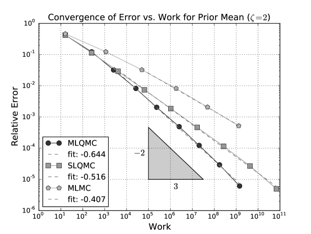
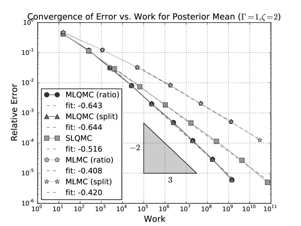
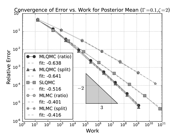
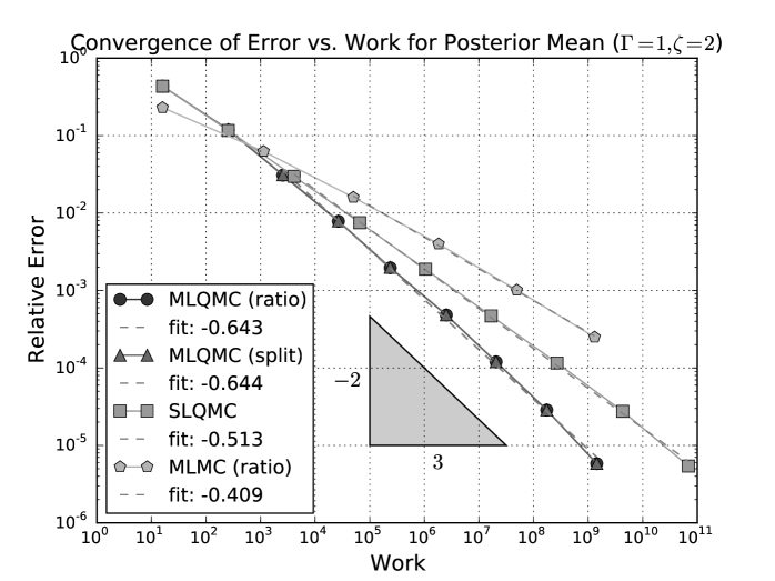
For Bayesian inversion, we consider as observation functional the integral over . This scalar value is perturbed by a realization of a normally distributed random variable as in (3.1) to generate a measurement, which is fixed for each value of before applying the various SL and ML HoQMC methods. For prior mean approximations, we compare the multilevel QMC method to the single-level QMC approach and to the multilevel Monte Carlo method. For approximations to the posterior expectation, we compare the performance of the analyzed multilevel QMC estimators (4.6), (4.10) with both the single-level QMC ratio estimator of [9] as well as the two multilevel estimators (4.6), (4.10) combined with standard Monte Carlo sampling. In all considered algorithms, we solve (5.8) by a Galerkin approximation based on continuous, piecewise linear finite elements on a family of uniform quadrilateral meshes with mesh width for , and we use interlaced polynomial lattice rules with points, , constructed by the fast CBC algorithm for SPOD weights from [6].
In the single-level HoQMC ratio estimator, the meshwidth is . The PG discretization error for regular functionals is, asymptotically, as , . We balance this discretization error with the dimension truncation error of and the HoQMC quadrature error of . These asymptotic error bounds yield the choices and , so that . Ignoring logarithmic factors, this yields a combined error of and overall cost of , with the constants implied in being independent of .
The HoQMC rules will be based on SPOD weights from [18]. A major finding of the single-level theory in [9] and of the multilevel error analysis in the present paper is that HoQMC rules which are efficient for forward UQ will perform equally well for the corresponding Bayesian Inverse UQ, due to preservation of holomorphy domains. We therefore use, in the affine parametric forward problem, the HoQMC weights derived in [6]. They are given by [6, Equation (3.32) with (3.17)] and
The generating vectors were computed by the fast CBC construction from [6] with Walsh constant . (computations with yielded different generating vectors, and led to slight artefacts on high levels in this example). For the presently used base , the choice holds [29].
In the multilevel algorithm in (4.7), (4.8), for given maximal discretization level , we take regular bisection refinement of the quadrilateral mesh in , resulting in a sequence of regular, quadrilateral meshes of with meshwidths for . We select the truncation dimension as as in (4.40), and as in (4.44), where for this particular case is given in Table 1.
| MLQMC | MLMC | |
|---|---|---|
| 0 | (1) | (1) |
| 1 | (3,1) | (5,2) |
| 2 | (5,3,1) | (10,7,4) |
| 3 | (7,5,3,1) | (15,11,8,5) |
| 4 | (9,7,5,3,1) | (19,15,12,9,7) |
| 5 | (11,9,6,5,3,2) | (24,20,16,13,10,8) |
| 6 | (13,11,8,6,5,3,2) | (28,24,20,17,14,11,9) |
| 7 | (15,13,10,8,6,5,3,2) | – |
| 8 | (17,15,12,10,8,6,5,3,2) | – |
Using formally the limiting values and , the total error is at cost of , ignoring logarithmic factors. For , we use the SPOD weights from the single-level case with from above. For , the SPOD weights that enter the fast CBC construction are different from those for the single-level algorithm; as indicated above, we use the choices derived for this problem in [6] for the affine-parametric forward problem also for the computation of integrals in the inverse problem. We take base , Walsh constant , and
6 Implementation and numerical results
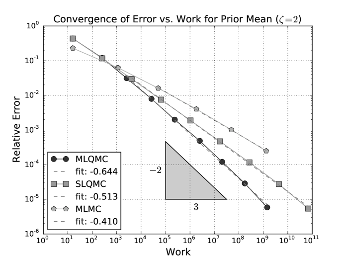
We now present numerical experiments which validate the choices of the algorithm steering parameters from Section 4.3.4 for their implementation, for the fast, deterministic solution of Bayesian inverse problems for PDEs with uncertain random field inputs. We present in particular experiments for the model linear, parametric elliptic forward problems from Section 5. The problems are set in the domain , with homogeneous Dirichlet boundary conditions, and with parametric coefficients given by an -term truncated Karhunen-Loève expansion in , with exactly known eigenfunctions. The first problem has an affine-parametric coefficient, the second problem is a nonlinear (holomorphic) transformation of this coefficient. The purpose of the ensuing numerical experiments is to illustrate the preceding convergence analysis and to show that the proposed MLHoQMC algorithms outperform other methods, such as MLMC, in terms of error vs. work. For the implementation, we use the gMLQMC library from [11].
We compute the forward solution up to maximal discretization level , yielding active dimensions. No exact solution for this problem is available, so we verify convergence rates by testing accuracy with respect to a numerically computed reference solution. This reference solution was computed on level with maximal truncation dimension and the MLQMC method. For the posterior expectation, the splitting estimator was used. In the error vs. work plot in the figures ahead, we used the work measures
| (6.1) |
The MLMC runs which are provided here for comparison purposes were performed with identical discretizations of the forward problems, and with the optimized MC sample numbers (4.45); in order to reduce the (inherent in MC sampling) scatter in the convergence rate plots, in the ensuing graphs the MLMC convergence was obtained by averaging MLMC runs. We emphasize that the presently considered MLHoQMC are entirely deterministic: for the MLHoQMC algorithms, the computation of each convergence plot required only one single run.
6.1 Affine parametric, linear elliptic test problem
In the results below, the work measures (6.1) were used for the multilevel methods. The expected convergence rate is for the single-level algorithm and for the multilevel algorithm (for both forward and inverse approximations), both of which are confirmed by the results. In the MLMC runs, repetitions were used to average out sampling noise in the estimated error. The MLQMC (splitting estimator) result with finest discretization level was used as a reference in the error computation.
6.2 Nonaffine-parametric, linear test problem
We consider once more the linear operator equation (5.8), however, now with diffusion coefficient modelled for by the nonlinear expression
| (6.2) |
i.e. simply the exponential of the affine-parametric coefficient model from (5.8) with , yielding for the new model the nominal value . When considering the exact same QMC parameters as for the above results () and maximal parameter dimension in the ML experiments being , we observe the results in Figures 5 to 7.
7 Conclusions
We extended [9] to a class of deterministic, multilevel Petrov-Galerkin, higher order Quasi-Monte Carlo integration algorithms for forward and Bayesian inverse computational uncertainty quantification of possibly nonlinear, well-posed operator equations. Novel, computable deterministic multilevel estimators have been proposed for “distributed” uncertain input data in a separable Banach space . Upon parametrizing the uncertain input data in terms of a countable basis of (as, e.g., through a Karhunen-Loève expansion), and upon multilevel Petrov-Galerkin discretization of the forward problems, the forward and Bayesian inverse uncertainty quantification problem is reduced to numerical evaluation of high-dimensional, parametric integrals of nonlinear functionals depending on the likelihood function of the responses from the parametric forward problem and the observation data. The numerical integration is conducted with the deterministic, higher order QMC integrations from [8]. The present results generalize, in particular, the HoQMC PG error analysis of [7] to smooth, nonlinear operator equations with holomorphic-parametric dependence of their responses on the parameters. They apply to broad classes of forward equations, with possibly indefinite or saddle point variational formulations, and nonlinear, analytic dependence on the parameters.
In several numerical experiments for Bayesian inversion of linear, elliptic forward problems in two space dimensions, the presently proposed, multilevel higher order Quasi Monte-Carlo strategy consistently outperformed the corresponding single-level algorithms from [9], and corresponding MLMC methods in both forward as well as Bayesian inverse UQ on parametric inputs with proper sparsity: to reach one percent accuracy in the Bayesian estimate, the MLHoQMC strategy achieves a speedup of a factor of error versus total work as compared to the SL strategy and to the MLMC approach. Higher efficiency is expected on input data with higher smoothness in the data space, i.e. , implies higher sparsity; having said this, we admit that for problems whose parametric input data does not afford sufficient sparsity, the presently proposed methods will not outperform MLMC and ML versions of first order QMC methods.
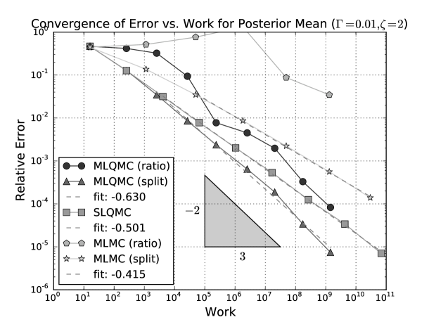
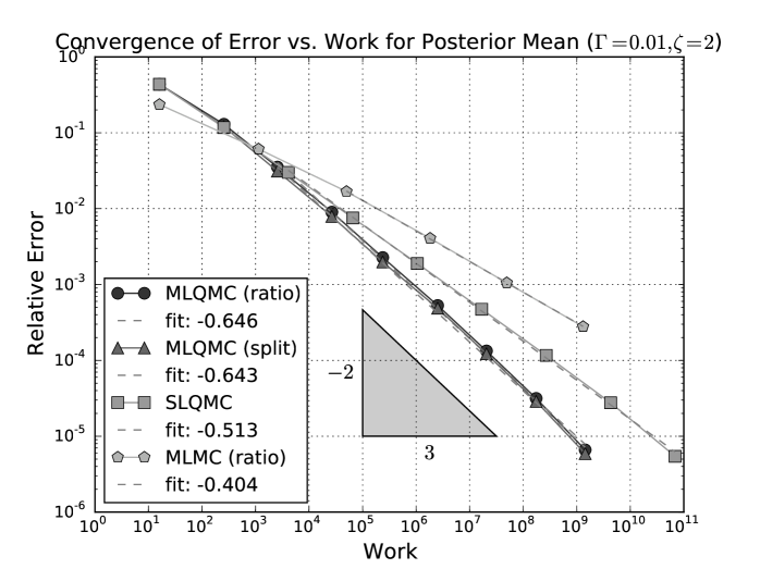
The presented numerical experiments also confirm the dimension-independence of the QMC convergence rates, which are only limited by input sparsity and by the digit interlacing order of the polynomial lattice rule. They also indicate the expected deterioration of the algorithms’ performance for small observation noise covariance ; in this respect, the splitting estimator was found to be less sensitive than the ratio estimator. The presently introduced algorithms allow us to handle uncertainties with several hundred to thousands of parameters, in two space dimensions, with moderate computational effort. The parametric sparsity of the countably parametric model problem considered in the numerical experiments was moderate ( in (5.12)); for classes of uncertain input data with higher sparsity, i.e. smaller values of , the gains of the presently proposed, HoQMC-based algorithms over MLMC are predicted to be correspondingly higher, as a consequence of the present theoretical results, and supported by extensive numerical experiments in [12].
Acknowledgments
This work was supported by CPU time from the Swiss National Supercomputing Centre (CSCS) under project IDs s522 and d41, by the Swiss National Science Foundation (SNF) under Grant No. SNF149819, by the European Research Council (ERC) under AdG 247277, and by Australian Research Council’s Discovery Project grants under project number DP150101770.
References
- [1] A. Beskos, A. Jasra, K. Law, R. Tempone and Y. Zhou, Multilevel Sequential Monte Carlo Samplers, Available at arXiv1503.07259v1.
- [2] F. Brezzi, J. Rappaz and P. A. Raviart, Finite dimensional approximation of nonlinear problmes I: Branches of nonsingular solutions, Numer. Math., 36 (1980), pp. 1–25.
- [3] A. Chkifa, A. Cohen and Ch. Schwab, Breaking the curse of dimensionality in sparse polynomial approximation of parametric PDEs. Journ. Math. Pures et Appliquees, 103, 400–428, 2015.
- [4] M. Dashti and A. M. Stuart, The Bayesian Approach to Inverse Problems (to appear in Handbook of Uncertainty Quantification, Springer Publ. 2016) Available at arXiv:1302.6989v4.
- [5] J. Dick, Walsh spaces containing smooth functions and Quasi-Monte Carlo rules of arbitrary high order. SIAM J. Numer. Anal., 46, 1519–1553, 2008.
- [6] J. Dick, F.Y. Kuo, Q. T. Le Gia, D. Nuyens and Ch. Schwab, Higher order QMC Galerkin discretization for parametric operator equations. SIAM J. Numer. Anal., 52, 2676–2702, 2014.
- [7] J. Dick, F.Y. Kuo, Q. T. Le Gia and Ch. Schwab, Multi-level higher order QMC Galerkin discretization for affine parametric operator equations. Report 2014-14 Seminar for Applied Mathematics, ETH Zürich, Switzerland (to appear in SIAM Journ. Numer. Analysis 2016). Available at arXiv:1406.4432
- [8] J. Dick, Q. T. Le Gia and Ch. Schwab, Higher order Quasi Monte Carlo integration for holomorphic parametric operator equations. Report 2014-23, Seminar for Applied Mathematics, ETH Zürich, Switzerland (to appear in SIAM Journ. Unc. Quantification 2016). Available at arXiv:1409.2180.
- [9] J. Dick, R. N. Gantner, Q. T. Le Gia and Ch. Schwab, Higher order Quasi-Monte Carlo integration for Bayesian Estimation. Report 2016-13, Seminar for Applied Mathematics, ETH Zürich, Switzerland (in review).
- [10] T.J. Dodwell, C. Ketelsen, R. Scheichl and A.L. Teckentrup, A Hierarchical Multilevel Markov Chain Monte Carlo Algorithm with Applications to Uncertainty Quantification in Subsurface Flow. SIAM/ASA Journal on Uncertainty Quantification, 3, 1075–1108, 2015.
- [11] R. N. Gantner, A Generic C++ Library for Multilevel Quasi-Monte Carlo. In Proceedings of the Platform for Advanced Scientific Computing Conference, PASC ’16, pages 11:1–11:12, New York, NY, USA, 2016. ACM.
- [12] R. N. Gantner and Ch. Schwab, Computational Higher Order Quasi-Monte Carlo Integration. In Monte Carlo and Quasi-Monte Carlo Methods 2014, R. Cools and D. Nuyens (eds.), Springer, Cham, pp. 271–288, 2016.
- [13] M. B. Giles, Multilevel Monte Carlo methods. Acta Numer., 24, 259–328, 2015.
- [14] V. Girault and P.A. Raviart, Finite Element Methods for Navier-Stokes Equations. Springer Verlag, Berlin, 1986.
- [15] M. Hansen and Ch. Schwab, Analytic regularity and best -term approximation of high dimensional, parametric initial value problems. Vietnam Journal of Mathematics, 41, 181–215, 2013.
- [16] H. Harbrecht, M. Peters, M. Siebenmorgen, Multilevel accelerated quadrature for PDEs with log-normally distributed diffusion coefficient. SIAM/ASA J. Uncertain. Quantif., 4, 520–551, 2016.
- [17] V. H. Hoang, Ch. Schwab and A.M. Stuart, Complexity analysis of accelerated MCMC methods for Bayesian inversion. Inverse Problems, 29, (8), 2013.
- [18] F. Y. Kuo, Ch. Schwab and I. H. Sloan, Quasi-Monte Carlo finite element methods for a class of elliptic partial differential equations with random coefficient. SIAM J. Numer. Anal., 50, 3351–3374, 2012.
- [19] F. Y. Kuo, Ch. Schwab and I. H. Sloan, Multi-Level Quasi-Monte Carlo finite element methods for a class of elliptic partial differential equations with random coefficient, Found. Comp. Math., 15, 411–449, 2015.
- [20] F. Kuo and R. Scheichl and Ch. Schwab and I. Sloan and E. Ullmann, Multilevel Quasi-Monte Carlo Methods for Lognormal Diffusion Problems, Report 2015-22, Seminar for Applied Mathematics, ETH Zürich (to appear in Mathematics of Computation).
- [21] J. Pousin and J. Rappaz, Consistency, stability, apriori and aposteriori errors for Petrov-Galerkin methods applied to nonlinear problems. Numer. Math., 69, 213–231, 1994.
- [22] Cl. Schillings and Ch. Schwab, Sparse, adaptive Smolyak quadratures for Bayesian inverse problems. Inverse Problems, 29, 065011, 28 pp, 2013.
- [23] Cl. Schillings and Ch. Schwab, Sparsity in Bayesian Inversion of Parametric Operator Equations. Inverse Problems, 30, 065007, 30 pp., 2014.
- [24] Cl. Schillings and Ch. Schwab, Scaling Limits in Computational Bayesian Inversion. Report 2014-26, Seminar for Applied Mathematics, ETH Zürich, (to appear in M2AN, 2016).
- [25] Ch. Schwab, QMC Galerkin discretizations of parametric operator equations. In J. Dick, F. Y. Kuo, G. W. Peters and I. H. Sloan (eds.), Monte Carlo and Quasi-Monte Carlo methods 2012, Springer Verlag, Berlin, 2013, pp. 613–630.
- [26] Ch. Schwab and C.J. Gittelson, Sparse tensor discretizations of high-dimensional parametric and stochastic PDEs. Acta Numerica, 20, 291–467, 2011.
- [27] Ch. Schwab and R. A. Todor, Karhunen-Loève approximation of random fields by generalized fast multipole methods. J. Comput. Phys., 217, 100–122, 2006.
- [28] A. M. Stuart, Inverse problems: a Bayesian perspective. Acta Numerica, 19, 451–559, 2010.
- [29] T. Yoshiki, Bounds on the Walsh coefficients by dyadic difference and a new Koksma-Hlawka type inequality for Quasi-Monte Carlo integration. Available at arXiv:1504.03175.