Pruning to Increase Taylor Dispersion in Physarum polycephalum Networks

Abstract

How do the topology and geometry of a tubular network affect the spread of particles within fluid flows? We investigate patterns of effective dispersion in the hierarchical, biological transport network formed by Physarum polycephalum. We demonstrate that a change in topology – pruning in the foraging state – causes a large increase in effective dispersion throughout the network. By comparison, changes in the hierarchy of tube radii result in smaller and more localized differences. Pruned networks capitalize on Taylor dispersion to increase the dispersion capability.

Transport due to fluid flowing through tubular networks is of great interest, because it has technological applications to biomimetic microfluidic devices Jr et al. (1999); Anderson et al. (2000); Kim et al. (2013), foams Cohen-Addad et al. (2013), fuel cells Coutelieris and Delgado (2013), and other filtration systems Yang (2003) and lies at the heart of extended organisms that rely on transport networks to function: animal vasculature Netti et al. (1997); Kapellos et al. (2010), fungal mycelia Boddy et al. (2009), and plant tubes Wu et al. (2010); Jensen et al. (2009); Williams et al. (2008). A big challenge regarding transport networks is to understand how network architecture changes the efficiency of particle spread throughout a network. While it is experimentally tedious to map particle transport in a network, predicting the spread of particles is also a theoretical challenge de Jong (1958); Saffman (1959); de Arcangelis et al. (1986); Lee et al. (1999); Bruderer and Bernabé (2001); Rhodes and Blunt (2006); Sahimi (2012); Iima and Nakagaki (2012). Attempts to understand how the network topology and geometry affect the transport of particles are scarce Bruderer and Bernabé (2001). Alternatively, we can study the dynamic changes of tubular network architecture in living beings. Organisms spontaneously reorganize their transport networks, including tube pruning Chen et al. (2012); Smith et al. (1992); Baumgarten et al. (2010, 2015). Examples are vessel development in zebra fish brain development Chen et al. (2012), or growth of a large foraging fungal body Smith et al. (1992). Here, we study the slime mold Physarum polycephalum  which emerged as an inspiring and yet puzzling model for ‘intelligent’ living transport networks.

P. polycephalum  like foraging fungi, actively adapts its network to environmental cues Nakagaki et al. (2000a, 2007); Nakagaki and Guy (2008); Dussutour et al. (2010); Tero et al. (2010). Networks connecting multiple food sources are a good compromise between efficiency, reliability, and cost, comparable to human transport networks Tero et al. (2010). Fluid cytoplasm enclosed in the tubular network exhibits nonstationary shuttle flows Kamiya (1950); Stewart and Stewart (1959); Isenberg and Wohlfarth-Bottermann (1976) driven by a peristaltic wave of contractions spanning the entire organism Alim et al. (2013). Investigations of transport in these networks are so far limited to estimates based on the minimal distance between tubes Tero et al. (2010); Fricker et al. (2009); Baumgarten and Hauser (2013). We tracked a well-reticulated individual trimmed from a larger network (Fig. 1). After several hours, the thin central tubes were abandoned in favor of a few large central tubes and globular structures at the periphery. How does this radical change of topology affect the transport capabilities of the individual? What role do hierarchical tube radii play?

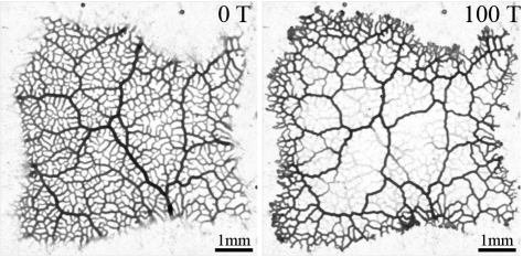
Figure 1: Bright-field image of a P. polycephalum individual cut from a larger network (left) and the same individual 100 contraction periods later (right).

We present a method to efficiently map the effective dispersion of particles from any initiation site throughout any network with nonstationary but periodic fluid flows. We use this method to study the change in dispersion patterns as an individual adjusts its morphology after trimming (Fig. 1). We find that the pruned state presents, on average, higher transport capabilities than the initial state. Emergent central tubes concentrate flow, enabling higher flow velocities across the entire network. Thus, the organism capitalizes on Taylor dispersion to increase particle spread. Finally, we study the influence of hierarchical tube radii by comparing hierarchical unpruned and pruned states to their theoretical counterparts with equal tube radii. We find that radial hierarchies influence dispersion patterns on local scales, but changes in average transport capabilities require pruning.

To prepare P. polycephalum networks, plasmodia from Carolina Biological Supplies were grown on 1.5% (wt/vol) agar without nutrients and fed daily with autoclaved oat flakes (Quaker Oats Company). A newly colonized oat flake was transferred to a fresh agar dish 8-24 h before imaging. Before imaging, slime mold networks were trimmed to remove growing fans and oat flakes. Bright-field microscopy images were obtained using a Zeiss Axio Zoom V16 stereomicroscope.

Network architectures were extracted with a Matlab program and discretized into $M$ nodes connected by $N$ tubes of length $\ell$ = 10px and measured average radius $a_{0,ij}$ ($ij$ designs the tube connecting vertices $i$ and $j$). Tubes of P. polycephalum undergo a peristaltic wave of contractions. Tube radii $a_{ij}(t)$ oscillate about $a_{0,ij}$ with contraction period $T$, inducing fluid flow $u_{ij}$ throughout the network. Given the network architecture and the periodic contractions, the flow throughout the network is computed by use of Kirchhoff’s law at every node, see Supplementary Information Sect. 1 for details.

To describe how quickly particles disperse from any given tube throughout a network, we want to quantify the growth rate of the area of a cloud of dispersing particles. After a short transient, the cloud disperses, on average, in a diffusive way, e.g. the radius squared of the cloud is proportional to time. We wish to evaluate that proportionality constant, that we call effective dispersion. For that we develop in the following a numerical method, the Dispersing Cloud, corresponding to a simplified resolution of the particle dynamics in the network. The method is most efficient to characterize the flow of particles in large networks.

The dispersion of particles due to fluid flow in a tubular network is, in general, a multidimensional problem. In the case of P. polycephalum, the tubes are long enough to smooth out variations in the concentration along the cross-section $\ell\gg ua_{0}^{2}/\kappa$. The cross-sectionally averaged concentration of particles $c(z,t)$ in each single tube is, thus, efficiently described by Taylor’s dispersion Taylor (1953); Aris (1956):

$$\frac{\partial c}{\partial t}=\frac{\partial}{\partial z}\left\{-uc+\left(\kappa+\frac{u^{2}a^{2}}{48\kappa}\right)\frac{\partial c}{\partial z}\right\}$$ (1)

where $\kappa=10^{-10}\rm{m^{2}/s}$ is the molecular diffusivity of particles. Fig. 2a) shows the evolution of the area of a cloud of dispersing particles starting from a single tube as described by Eq. 1. Solving Eq. 1 for all starting points in the trial network considered (inset of Fig. 2a) takes several days and is thus unreasonable for large networks.

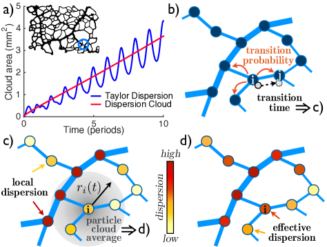
Figure 2: a) Change in the area of a cloud of dispersing particles, according to the numerical solution of the full Taylor dispersion and the dispersion cloud method, for the starting point circled in blue; see network inset. b) Particles spread in a random walk defined by transition probabilities and times, allowing the definition of local dispersion coefficients. c) Particles effectively spread as a Gaussian cloud of radius $r_{i}$ from site $i$, with a rate averaged over the local dispersions. This method yields the effective dispersion at long time scales in d).

To capture the trend of these dispersion dynamics with time in a more succinct way, we first aim at deriving the local dispersion properties in the network. After that step, calculating the long time dynamics will require only a subtle averaging of these local dispersion properties over time. Thinking of the dispersion dynamics as a random walk of particles, we write the local dispersion, representing the instantaneous diffusion coefficient at node $i$, as:

$$D_{i}=\sum_{k\in\mathrm{nn}(i)}p_{ik}\frac{\ell^{2}}{2t_{ik}}$$ (2)

where $nn(i)$ are the nearest node neighbors of $i$, $p_{ik}$ is the average probability of entering tube $ik$, and $t_{ik}$ is an average transition time in that tube, see Fig. 2b, and c. The transition probability and time are determined by the flow dynamics, in the spirit of Saffman (1959). We introduce time-independent quantities by averaging variables over the period of the oscillations $T$. For a particle at node $i$, the probability of entering one of the connected tubes nn($i$) is proportional to the flux at the entry of that tube. We thus define $p_{ij}=q_{\mathrm{rms},ij}/\sum_{k\in\mathrm{nn}(i)}q_{\mathrm{rms},ki}$, where $q_{\mathrm{rms},ij}$ is the time-averaged root mean square flux in tube $ij$. The transition time is the minimum of either diffusion-dominated or advection-dominated transport: $t_{ij}=\min(t_{\mathrm{diff},ij},t_{\mathrm{adv},ij})$. We take the effective diffusivity in Eq. 1 to determine the diffusion-dominated transition time to be:

$$t_{\mathrm{diff},ij}=\frac{\ell^{2}}{2}\left\langle\frac{1}{\kappa+\frac{u_{ij}^{2}a_{ij}^{2}}{48\kappa}}\right\rangle_{\ell,T},$$ (3)

where we average along the entire tube of length $\ell$ and over the period $T$. Averaging over the period is justified because the period is small compared to the time scales we are interested in. To compute the time it takes a particle to transverse a tube by advection we in general have to solve for the trajectory of the particle at any given start time $t_{0}\in T$,

$$\frac{dz(t)}{dt}=u_{ij}(z,t),\;z(t_{0})=0,\;z(t_{0}+t_{\mathrm{adv},ij}(t_{0}))=\ell.$$ (4)

For stationary flows the advection time is simply $t_{\mathrm{adv},ij}=u_{ij}/\ell_{ij}$. For the nonstationary flows arising from the peristaltic wave in P. polycephalum we analytically solve Eq. 4 by approximating the oscillatory flow velocities with $u_{ij}\approx u_{0,ij}\cos(\omega(t-t_{0}))$, where $u_{0,ij}^{2}=2\left\langle u_{ij}^{2}\right\rangle_{T}$. The diffusive time scale defined by Eq. 3 acts as a cutoff for tubes in which the fluid velocity is insufficient to allow a particle to traverse the tube before the flow reverses, e.g. when Eq. 4 has no solution.

Based on these local dispersion properties, we now define laws for the evolution of the area $r_{i}^{2}$ of a cloud of particles spreading from an initial node $i$, and define the effective dispersion after the transient initial phase as

$$\mathscr{D}_{i}=\lim_{t\gg T}\frac{r_{i}^{2}(t)}{4t},$$ (5)

where the limit indicates times that are large, compared to the initial transition time. At this point effective dispersion saturates; in most of our individuals saturation is reached after a few periods. Effective dispersion thus describes the growth of the radius of a cloud of particles from initiation node $i$ with $\sqrt{4\mathscr{D}_{i}t}$ to the boundary of the network. We assume that the probability of finding a particle at a Euclidian distance $d$ from node $i$ is proportional to a circular Gaussian: $\left(2\pi r_{i}^{2}\right)^{-1/2}\exp(-2d^{2}/2r_{i}^{2})$, with $r_{i}^{2}=4D_{i}t$ Gardiner (1985). Over time the cloud reaches nodes that have different local dispersion properties, and thus $r_{i}^{2}$ grows with the average over the local dispersion coefficients within the cloud, weighted by the probability of finding particles at that point:

$$\delta r_{i}^{2}=\frac{4\delta t}{K}\sum_{m\neq i}\frac{D_{m}}{\sqrt{2\pi r_{i}^{2}}}\exp\left(-\frac{d^{2}_{im}}{2r_{i}^{2}}\right),$$ (6)

where $d_{im}$ denotes the Euclidean distance between nodes and $K=\sum_{m\neq i}\left(2\pi r_{i}^{2}\right)^{-1/2}\exp(-\frac{d^{2}_{im}}{2r_{i}^{2}})$ is a normalization factor, see Fig. 2c and d. In flows with a net drift the Gaussian center would move with that drift velocity. Effective dispersion takes the detailed geometry of the network into account. As depicted in Fig. 2d), a node with low local dispersion coefficient $D_{i}$, but close to a node with a high $D_{j}$ has a high effective dispersion $\mathscr{D}_{i}$. Iteratively solving for the variance of the dispersing cloud of particles still reproduces the solution for Taylor dispersion on a network very well, see Fig. 2a) (and Supplementary Information Fig. S2). The computation of the dispersing cloud with the method of Eq. 6 for any starting point over the entire trial network of Fig. 2a) takes only a few minutes.

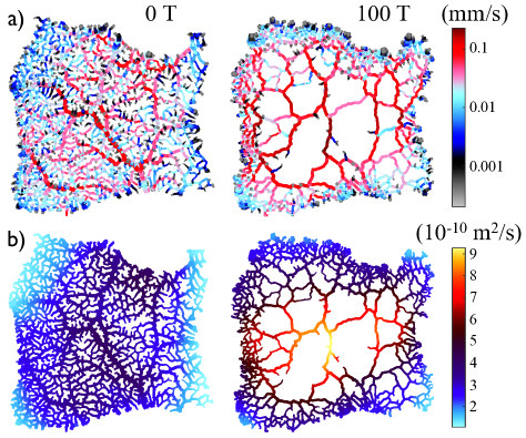
Figure 3: a) Maps of the root mean square flow velocity, and b) effective dispersion, for the initial network (left) and the same individual 100 contraction periods later (right).

The concept of effective dispersion allows us to efficiently parse how quickly particles will spread from any location within a large transport network. We use this method on P. polycephalum individuals (Fig. 1) to show that pruning - a change in the topology of the network - significantly enhances global network transport capabilities (Fig. 3). In an unpruned network, the flow pattern is high along the direction of the peristaltic wave (top left to bottom right) growing to its highest values at the network’s center. In the pruned network, the flow is high in all central tubes. The mass accumulated in all of the many peripheral tubes has to pass through only a few central tubes, and so the velocity in these tubes is higher than in the unpruned network. As expected from Taylor dispersion Eq. 1, tubes with high flux enable particles to spread effectively. On average over the network - weighted by the volume of the tubes -, effective dispersion for the pruned case is $36\%$ higher than in the unpruned case, being notably higher at the center. This result is qualitatively conserved among independent experiments (see Supplementary Information Sect. 3). Pruning capitalizes on Taylor dispersion to enhance transport. Although flow maps are only slightly different, effective dispersion maps reveal differences. The large central tubes of the unpruned and pruned networks have comparable flow velocities and sizes, yet the proximity of numerous small tubes in the unpruned case decreases effective dispersion by about a factor of two. In the pruned network, particles do not get lost in the more slowly propagating, smaller central tubes found in the unpruned network, and can be efficiently flushed further away.

The topological changes to a network imposed by pruning appear to be the limiting case of geometrical changes to the hierarchy of tube radii. We demonstrate now that geometric changes in a network can impose heterogeneous transport capabilities, but large changes in overall effective dispersion require pruning. To assess the impact of a hierarchical organization of tubes we compare the dispersion properties of pruned and unpruned states (ii) to a reference, nonhierarchical network with equal radii but the same overall mass (i), see Fig. 4. In an unpruned network, (a), average effective dispersion is about $11\%$ higher when radii have no hierarchy, and in a pruned network, (b), the difference is less than $1\%$. These results also translate qualitatively to other individuals (see Supplementary Information Sect. 3). Maps of effective dispersion in the unpruned network reveal that a hierarchical organization localizes regions of high transport capabilities along and near larger central tubes, rather than homogeneous patterns of dispersion, as found in the reference nonhierarchical network. In the pruned network, a hierarchical organization enhances the dispersal properties of the center, while the spreading efficiency in peripheral tubes is barely impacted. Yet, the measured change in effective dispersion may explain previously observed changes in the mixing rate with network geometry Nakagaki et al. (2000b).

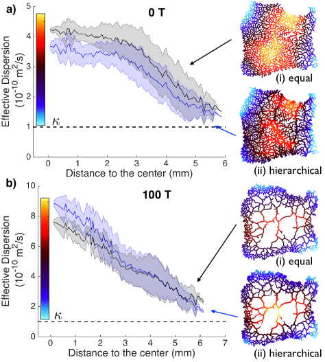
Figure 4: Average effective dispersion as a function of distance to the center for unpruned (a) and pruned (b) states (shaded areas mark standard deviations). The base dashed line represents the molecular diffusivity $\kappa=10^{-10}\rm{m^{2}/s}$. Note the difference in scales. Blue and black curves represent data from hierarchical (ii) and nonhierarchical cases (i), respectively. Insets are colored to show effective dispersion.

In summary, we investigated the impact of topology and geometry on particle flow within a live, tubular network by observing P. polycephalum. By introducing the concept of effective dispersion, we provide an efficient method to map how quickly particles disperse throughout a transport network from any initiation site. Effective dispersion measures the growth rate of an area of dispersing particles, and can be used for any stationary or nonstationary but periodic flow. Regarding the analysis of transport network properties, effective dispersion gives a faithful yet efficient mapping of flow-driven transport dynamics that are only to a certain extent captured by measures like “betweenness” Newman (2001); Goh et al. (2001) and mean first passage time measures Tejedor et al. (2011). We employed the effective dispersion method to compare an initially well-reticulated network formed by P. polycephalum with its evolved state 100 contraction periods later. We observe that an alteration of network topology, massive pruning, leads to a significant increase in global effective dispersion. The remaining large tubes serve as bottlenecks for flows. Capitalizing on Taylor dispersion, particle diffusivity is strongly enhanced not only at the center but throughout the network. By comparison, changes in the geometry of a network caused by a hierarchical organization of tube radii, while inducing specific zones of high transport capabilities, overall have a smaller impact on effective dispersion than pruning. By observing P. polycephalum we learned that pruning increases transport properties tremendously. It is fascinating to speculate that pruning in other biological systems, for example, during vessel development in zebra fish brain development Chen et al. (2012) or during growth of a large fungal body Smith et al. (1992), serve a similar objective of enhanced effective dispersion. Pruning itself might be triggered by the concentration of specific dispersing particles. Pruning is also tightly governed by the initial pattern of hierarchy, and the dynamic entanglement between hierarchy and pruning remains unsolved. Investigating the mechanisms allowing for pruning would be highly instructive in the process of understanding the overall organization of organisms.

in 1,…,11 See pages \x, of Supplemental.pdf