Outflow and metallicity in the broad-line region of low-redshift active galactic nuclei

Abstract

Outflows in active galactic nuclei (AGNs) are crucial to understand in investigating the co-evolution of supermassive black holes (SMBHs) and their host galaxies since outflows may play an important role as an AGN feedback mechanism. Based on the archival UV spectra obtained with HST and IUE, we investigate outflows in the broad-line region (BLR) in low-redshift AGNs ($z<0.4$) through the detailed analysis of the velocity profile of the C IV emission line. We find a dependence of the outflow strength on the Eddington ratio and the BLR metallicity in our low-redshift AGN sample, which is consistent with the earlier results obtained for high-redshift quasars. These results suggest that the BLR outflows, gas accretion onto SMBH, and past star-formation activity in the host galaxies are physically related in low-redshift AGNs as in powerful high-redshift quasars.

I. INTRODUCTION

It is widely believed that a supermassive black hole (SMBH) resides at the central part of most massive galaxies, and the mass of SMBHs ($M_{\rm BH}$) reaches up to $\sim$$10^{10}M_{\odot}$ (e.g., Vestergaard et al. 2008; Schulze & Wisotzki 2010; see also Wu et al. 2015). Interestingly, scaling relations have been observed between the SMBH mass and physical properties of their host galaxies, regardless of AGN activity (e.g., Magorrian et al., 1998; Ferrarese & Merritt, 2000; Gebhardt et al., 2000; Marconi & Hunt, 2003; Häring & Rix, 2004; Kormendy & Ho, 2013; Woo et al., 2013, 2015), suggesting that SMBHs and galaxies evolved with a close interaction (e.g., Merloni et al. 2004). However, the physics behind the co-evolution is unclear, preventing us from full understandings of the cosmological evolution of galaxies and SMBHs.

The gas accretion onto SMBHs is a fundamental process to explain the origin of the huge luminosity of active galactic nuclei (AGNs). Since AGNs are often associated with the star formaiton in their host galaxies (e.g., Heckman et al. 1997; Cid Fernandes et al. 2001; Netzer 2009; Woo et al. 2012; Matsuoka & Woo 2015), AGNs are a key population to explore the SMBH-galaxy co-evolution. More recent works suggest that AGN activity is important to quench star formation in their host galaxies (the negative AGN feedback; see, e.g., Kauffmann & Haehnelt 2000; Granato et al. 2004; Di Matteo et al. 2005; Croton et al. 2006; Hopkins et al. 2006; Ciotti et al. 2010; Scannapieco et al. 2012; cf. for positive AGN feedback, see, e.g., Silk 2005; Gaibler et al. 2012; Zubovas et al. 2013; Ishibashi et al. 2013) then the quenching of the star-forming activity is expected to terminate the AGN activity. Therefore the AGN feedback is now regarded as a crucial process for the SMBH-galaxy co-evolution.

Outflows are often considered as one of the AGN feedback mechanisms. The velocity profile and shift from the systemic velocity of various absorption and emission lines observed in UV and optical spectra of AGNs suggest the presence of the strong outflow of ionized gas, that exist in both small spatial scales corresponding to the broad-line region (BLR, that is located at the sub-pc scale from the nucleus) and large spatial scales corresponding to the narrow-line region (NLR, that is located at $\sim$$10^{1-4}$ pc from the nucleus) (Weymann et al., 1991; Crenshaw et al., 2003; Ganguly et al., 2007; Müller-Sánchez et al., 2011; Harrison et al., 2014; Bae & Woo, 2014; Husemann et al., 2016; Woo et al., 2016; Karouzos et al., 2016; Woo et al., 2017). Not only the ionized gas, powerful outflows of molecular gas at the scale of their host galaxies are also seen in sub-millimeter and millimeter spectra (e.g., Maiolino et al., 2012; García-Burillo et al., 2014). The inferred kinetic power of AGN outflows is high enough ($\sim 10^{43-45}$ erg s^-1; e.g., Tombesi et al. 2012) that a large amount of ISM in AGN host galaxies can be blown away, resulting in the termination of the star-formation activity. However, the detailed properties and physical origin of the AGN outflow are not understood well, and thus further observational studies on the AGN outflow is crucial to reveal the nature of the AGN feedback.

Though the AGN outflow is seen in various spatial scales as described above, the BLR has been particularly investigated to examine the nature of the AGN outflow. Especially high-ionization emission lines from BLRs such as C IV$\lambda$1549 are interesting for assessing the BLR outflow. This is because those high-ionization lines are emitted from the closer region to the AGN central engine than low-ionization lines, such as Mg II, as suggested by reverberation mapping observations (e.g., Clavel et al., 1991; Sulentic et al., 2000; Wang et al., 2012) and also by photoionization models (e.g., Baldwin et al., 1995; Korista & Goad, 2000). In fact, the C IV emission line sometimes show significant blueshifts (Gaskell, 1982; Wilkes, 1984; Marziani et al., 1996; Sulentic et al., 2000; Vanden Berk et al., 2001; Richards et al., 2002; Baskin & Laor, 2005; Sulentic et al., 2007) or asymmetric velocity profiles (Sulentic et al., 2000; Baskin & Laor, 2005; Sulentic et al., 2007) than low-ionization BLR lines. It has been also reported that the outflow properties in BLRs are also related to the Eddington ratio (e.g., Wang et al., 2011). In terms of the SMBH-galaxy co-evolution, the relation between the AGN outflow properties and the metallicity is specifically important because the metallicity is strongly linked to the past star-formation history of the host galaxy. Wang et al. (2012) reported the close relation between the BLR metallicity ($Z_{\rm BLR}$) and AGN outflow through the analysis of the C IV emission-line profile in a SDSS high-$z$ ($1.7<z<4.0$) QSO sample, and concluded that the past star formation in galaxy could affect both the accretion activity and the AGN outflow in the BLR scale.

There is a limitation in the observational studies of the AGN outflows; the BLR outflow has been explored often for high-redshift QSOs (e.g., Crenshaw et al., 2003; Wang et al., 2011, 2012). This is because high-ionization BLR lines such as C IV are in the rest-frame UV and thus they are not observable from ground-based telescopes. The lack of systematic studies of the BLR outflow at low-redshift Universe prevents us from examining the redshift evolution of the outflow, that is crucial to understand the role of AGN feedback within the context of the SMBH-galaxy co-evolution in the cosmological timescale. Another motivation for the BLR outflow study in low-redshift AGNs is from the expectation that the basic properties and physics of the AGN outflow could be different between high redshift and low redshift, since the typical gas fraction of host galaxies is expected to be completely different between high-redshift and low-redshift AGNs (Daddi et al., 2010; Tacconi et al., 2010; Geach et al., 2011; Bauermeister et al., 2013; Tacconi et al., 2013; Popping et al., 2015).

Shin et al. (2013) presented rest-frame UV spectra of 70 low-redshift ($z<0.5$) PG QSOs for investigating the relation between $Z_{\rm BLR}$ and AGN properties such as the SMBH mass, AGN luminosity, and Eddington ratio. This sample is extremely useful also for studying the nature of the BLR outflow in low-redshift AGNs, especially for examining possible relations between the outflow activity and the metallicity in the BLR scale. Therefore, in this paper, we investigate the BLR outflow for the sample of PG QSOs given in Shin et al. (2013). The structure of this paper is as follows. We describe the sample selection and the data in §2, and then explain the data analysis especially on the determination of some outflow indicators in §3. The main results are presented in §4, followed by the discussion in §5. Finally, the summary and conclusions are given in §6. We adopt a cosmology of $H_{\rm 0}=70$ km s^-1 Mpc^-1, $\Omega_{\Lambda}=0.7$ and $\Omega_{\rm m}=0.3$.

Table 1The archival UV data used in this study

Target ID	Redshift	Observation Date	Telescope/Instrument
(1)	(2)	(3)	(4)
Mrk 106	$0.123$	2011 May 12, 13	HST/COS
Mrk 110	$0.035$	1988 Feb 28	IUE/SWP
Mrk 290	$0.030$	2009 Oct 28	HST/COS
Mrk 493	$0.031$	1996 Sep 04	HST/FOS
Mrk 506	$0.043$	1979 Jul 03	IUE/SWP
Mrk 1392	$0.036$	2004 Jun 07	HST/STIS
PG 0157+001	$0.164$	1985 Aug 09	IUE/SWP
PG 0921+525	$0.035$	1988 Feb 28,29	IUE/SWP
PG 0923+129	$0.029$	1985 May 01	IUE/SWP
PG 0947+396	$0.206$	1996 May 06	HST/FOS
PG 1022+519	$0.045$	1983 May 31; Jun 01	IUE/SWP
PG 1048+342	$0.167$	1993 Nov 13	IUE/SWP
PG 1049-005	$0.357$	1992 Apr 01,	HST/FOS
PG 1115+407	$0.154$	1996 May 19	HST/FOS
PG 1121+422	$0.234$	1995 Jan 08	IUE/SWP
PG 1151+117	$0.176$	1987 Jan 29, 30	IUE/SWP
PG 1202+281	$0.165$	1996 Jul 21	HST/FOS
PG 1229+204	$0.063$	1982 May 01, 02	IUE/SWP
PG 1244+026	$0.048$	1983 Feb 08	IUE/SWP
PG 1307+085	$0.155$	1980 May 04	IUE/SWP
PG 1341+258	$0.087$	1995 Mar 22	IUE/SWP
PG 1404+226	$0.098$	1996 Feb 23	HST/FOS
PG 1415+451	$0.114$	1997 Jan 02	HST/FOS
PG 1425+267	$0.366$	1996 Jun29	HST/FOS
PG 1427+480	$0.221$	1997 Jan 07	HST/FOS
PG 1444+407	$0.267$	1996 May 23	HST/FOS
PG 1448+273	$0.065$	2011 Jun 18	HST/COS
PG 1512+370	$0.371$	1992 Jan 26	HST/FOS
PG 1519+226	$0.137$	1995 Jun 11	IUE/SWP
PG 1534+580	$0.030$	2009 Oct 28	HST/COS
PG 1545+210	$0.266$	1992 Apr 08, 10	HST/FOS
PG 1552+085	$0.119$	1986 Apr 28	IUE/SWP
PG 1612+261	$0.131$	1980 Sep 10	IUE/SWP
PG 2233+134	$0.325$	2003 May 13	HST/STIS

Note. — Col. (2): Redshift adopted from the NED.

II. Sample Selection and the Data

As mentioned in §1, high-ionization emission lines from the BLR seen in the rest-frame UV spectrum are generally used to study the AGN outflow in the sub-pc scales. We focus on the C IV line in this work, since other high-ionization BLR lines are heavily blended with other lines (e.g., N V$\lambda$1240, O IV]$\lambda$1402) or too weak to investigate in detail (e.g., N IV]$\lambda$1486, He II$\lambda$1640). In addition to C IV, optical emission lines from the NLR are necessary in the outflow analysis to define the reference redshift (see §3.1 for more details). Therefore we need a sample of AGNs whose UV and optical spectra with a high signal-to-noise ratio are available.

In Shin et al. (2013), flux ratios of UV emission lines from BLRs in 70 PG QSOs at $z<0.5$ were measured for studying $Z_{\rm BLR}$. Objects with broad absorption-line (BAL) features were excluded, for accurate measurements of the emission line fluxes. Among these 70 PG QSOs, 31 objects have optical spectra in the data-archive of the Sloan Digital Sky Survey (SDSS; York et al., 2000). Since three objects show no strong NLR lines in their SDSS spectra, we select 28 PG QSOs with optical NLR spectra. Then we enlarge the sample size by examining the Markarian sample from the 13th Veron-Cetty AGN catalog Véron-Cetty & Véron (2010). Among 241 Markarian AGNs, 30 objects have available UV and optical spectra. Through our visual inspection, we select 6 Markarian objects whose UV and optical spectra show high enough signal-to-noise ratios for our analysis and show no BAL features. Therefore, we finalize sample that consists of 28 PG QSOs and 6 Markarian AGNs (34 non-BAL AGNs in total, see Table 1). The mean, standard deviation, and median of the redshift of 34 AGNs in our sample are 0.14, 0.11, and 0.13 respectively.

The UV spectra of our sample are retrieved from the Mikulski Archive for Space Telescopes (MAST). They were obtained with Cosmic Origins Spectrograph (COS), Space Telescope Imaging Spectrograph (STIS), or Faint Object Spectrograph (FOS) on board Hubble Space Telescope (HST), or the short-wavelength-prime (SWP) detector on board International Ultraviolet Explorer (IUE). If there are multiple data sets taken with different telescopes, we use higher resolution data in order of COS ($R\sim 16000-21000$), STIS ($R\sim 11400-17400$), FOS ($R\sim 1300$), and IUE ($R\sim 300$). For some targets which were observed multiple times with the same instrument at similar epochs, we combine their spectra by calculating error-weighted mean to obtain their spectra with a better signal-to-noise ratio. For STIS and COS spectra, we perform 2 pixel boxcar smoothing for STIS spectra and 7 pixel boxcar smoothing for COS spectra since these spectra are highly over-sampled; i.e., the pixel scale is $\sim$ 0.05Å/pixel for STIS spectra and $\sim$ 0.012Å/pixel for COS spectra, compared to the spectral resolution elements.

For given a large difference of spectral resolution between HST and IUE observations, we consider the effect of spectral resolution on the kinematic measurements from emission lines. To examine whether our analyses are sensitive to the spectral resolution, we convolve two COS spectra (Mrk 106 and PG 1534+580) with a series of Gaussian kernels, to artificially decrease the spectral resolution. Using each of these spectra, we re0fit the emission lines. We find that the outflow parameters (see §3.1) and emission-line flux ratios used in our analyses are not sensitive to the spectral resolution, up to the spectral resolution $R\sim 1000$. As expected emission line flux ratios do not depend on the resolution and the kinematic measurements are consistent within $\sim$3-10%.

The optical spectra of our sample are retrieved from the SDSS Data Release 7 (DR7; Abazajian et al., 2009). The broad wavelength coverage of SDSS spectra (3800–9200Å) enables us to detect various narrow emission lines (i.e., the [O ii] doublet emission at 3727.09Å and 3729.88Å, the [O iii] doublet emission at 4960.30Å and 5008.24Å, and the [S ii] doublet emission at 6718.32Å and 6732.71Å) for low-redshift AGNs. These narrow lines are used for the accurate redshift determination. Also, we can quantify various AGN properties such as the black hole mass and AGN bolometric luminosity using broad H$\beta$ line and 5100Å continuum luminosity. Details of our analysis on the SDSS optical spectra will be presented in §3.

Table 1 shows the details of the UV data (observing data, telescope, and instrument) for each object. Though the redshift given in Table 1 are taken from the NASA/IPAC Extragalactic Database (NED), we do not simply use those redshift for our analysis, (see §3.1).

III. Analysis

III.1. Outflow indicators and redshift determination

The BLR outflow is recognized through velocity profiles of broad emission lines in AGN spectra, characterized by the asymmetry or blueshift with respect to the systemic velocity of the object (e.g. Sulentic et al., 2000). Each of the asymmetry and relative blueshift can be quantified straightforwardly based on observed emission-line spectra (e.g., Sulentic et al., 2000; Baskin & Laor, 2005; Sulentic et al., 2007; Wang et al., 2011). Wang et al. (2011) proposed a new indicator, the blueshift and asymmetry index (BAI), that takes account of both the asymmetry and relative blueshift of emission lines (see also Wang et al., 2012). In our analysis, we investigate 3 parameters to quantify the strength of the AGN outflow at the BLR; the asymmetry index, the velocity shift index, and BAI.

The asymmetric index (AI) is defined as the flux ratio between the blue part from the C IV profile peak and the total (Eq. 1). The velocity shift index (VSI) is defined by the velocity difference between the C IV profile peak and the laboratory center of the C IV emission, 1549.06Å, which is the oscillator strength weighted average wavelength of the two C IV doublet lines at 1548.20Å and 1550.77Å (Eq. 2; see, e.g., Vanden Berk et al., 2001). The C IV BAI, which combines the blueshift and asymmetric effects in the C IV velocity profile, is the flux ratio between the blue part from the C IV laboratory center and the total (Eq. 3). These indices are expressed by the following equations:

$$AI=\frac{F\rm{(Blue\ region\ from\ the\ CIV\ peak)}}{F\rm{(Total\ CIV)}}$$ (1)

$$VSI=v{\rm(CIV\ peak)}-v{\rm(CIV\ lab)}$$ (2)

$$BAI=\frac{F{\rm(Blue\ region\ for\ the\ CIV\ laboratory\ wavelength)}}{F{\rm(Total\ CIV)}}$$ (3)

For determining VSI and BAI, the systemic redshift is crucial otherwise the laboratory location of C IV is not known. In principle, the best way to measure the systemic redshift of galaxies is to use stellar absorption-line features (e.g., Bae & Woo, 2014; Woo et al., 2016). Although measuring systematic redshift from stellar absorption-line is very challenging in type 1 AGNs due to strong AGN continuum emission (but see, e.g., Woo et al., 2008; Harris et al., 2012; Park et al., 2012b, 2015; Woo et al., 2015), we try to measure stellar absorption lines (Mgb, Fe ii]$\lambda$5270, CaII triplet, and Ca H&K lines) in SDSS spectra of our sample by using Penalized Pixel-Fitting method (PPXF code Cappellari & Emsellem, 2004). This does not provide a good constraint, mainly due to insufficient signal-to-noise ratios of the SDSS spectra. Therefore we have to focus on some emission-line features, instead of stellar features, to determine the systemic redshift of each object.

Sometimes the UV Mg II emission line from the BLR is used to determine the systemic redshift of type 1 AGNs (e.g., Richards et al., 2002), because the Mg II line is one of strong low-ionization emission lines from the BLR and thus less affected by nuclear radial motions of gas outflows as already mentioned in §1. However we do not use the Mg II line for determining the systemic redshift, because some of the UV spectra of our sample do not cover the Mg II line. Another reason is that the total mass of the BLR gas is only tiny with respect to the host galaxy (e.g., Baldwin et al., 2003) and thus could be easily affected by possible radial motions. Some observations actually report that the Mg II-based redshift shows systematic differences from the systemic redshift (e.g., based on [O III] line; McIntosh et al. 1999; Vanden Berk et al. 2001).

More appropriate features than the Mg II line to determine the systemic redshift are narrow optical emission lines from NLRs, since the NLR resides at much large spatial scales (e.g., Bennert et al., 2006a, b) with a larger total gas mass than the BLR (e.g., Fraquelli et al., 2003; Crenshaw et al., 2015). In the previous studies, [O III] line is used to determine the systemic redshift (e.g., Hewett & Wild, 2010). However high-ionization NLR lines such as [O III] sometimes show asymmetric velocity profiles due to radial gas motions (e.g., Komossa et al., 2008; Bae & Woo, 2014; Woo et al., 2015, 2016), because such relatively high-ionization NLR lines arise at the innermost part of NLRs in AGNs (e.g., Nagao et al. 2000, 2001) and thus easily affected by the outward pressure due to the AGN radiation. Therefore, in this work, we use low-ionization lines for determining the systemic redshift. Specifically, we use the [S II]  [O II], [O I], and H$\beta$ emission lines in this study. We fit those lines in the SDSS spectra by adopting a simple Gaussian profile. For the [S II] (at 6718.29Å and 6732.67Å in the laboratory) and [O I] (at 6302.05Å and 6365.5Å) doublet emissions, we fix their wavelength separations and widths. We treated the [O II] emission as a single Gaussian line at 3728.48Å (the average of the two doublet line wavelengths), because the [O II] doublet lines are heavily blended in most cases. As for the H$\beta$ and [O III] wavelength region, we subtract the blended Fe II multiplet and stellar emission before the narrow-line measurement. Note that the subtraction of the Fe II and stellar emission is important not only for the NLR fitting but also for measuring the velocity dispersion of the broad H$\beta$ emission for the estimate of $M_{\rm BH}$ (see §3.2). We use the Fe II template given by Tsuzuki et al. (2006), and the host galaxy template given by Bruzual & Charlot (2003), a following procedures described in (Park et al., 2012b, 2015). After decomposing the broad component of H$\beta$ with sixth-order of Gauss-Hermitian series, we fit the narrow component of H$\beta$ and [O III] with the single Gaussian. We do not use [N II] emission lines since it is buried by the broad H$\alpha$ line in most objects in our sample.

Using the measured central wavelength of each NLR line, we then calculate the systemic velocity (reference redshift), respectively, and estimate BAI and VSI, using the peak of C IV line from the best-fit model. To obtain the outflow and metallicity indicators, we fit emission lines in our interest, namely, C IV, N V, Si IV, O IV], and He II by adopting multi component fitting method (see also Shin et al., 2013). First, we divide BLR lines into two groups based on the ionization potential, and assume that all emission lines in the same group have the same emission-line profile. Second, we mask out narrow absorption lines present in some targets. Third, we adopt a double Gaussian profile, which well reproduces the observed BLR emission lines. Here we assume that both Gaussian components are originated from the BLR since the velocity width of the narrower Gaussian component is wider than 1500 km s^-1 in most cases, while the contribution of the NLR emission to the CIV profile seems not significant as we do not detect them in our fitting analysis. Although it is possible that there is a weak narrow C IV component, the effect of this component on our results is presumably insignificant. As we expect, high ionization emission lines (N V, C IV, O IV], He II) are well fitted with the same line profile, suggesting that other high ionization emission lines also show strong outflow as well as C IV. However, N V, O IV], He II are blended with other emission lines. Thus, we use C IV to avoid any systemic uncertainty due to the deblending.

In Figure 1, we compare the BAIs obtained with adopting different reference lines for a consistency check. All VSIs measured based on each redshift reference line are correlated with each other with only small scatters, showing that there are no significant systematic difference among the VSIs derived from other emission lines. The scatter is mostly within a few tens km $\rm s^{-1}$ except for the cases when the redshift given in the NED is adopted. In the following analysis we exclude the reference redshift adopted from the NED. Instead, we decide to adopt the redshift reference in order of [S II], [O I], [O II], and H$\beta$, if not all lines are available. This order is determined based on the line strength and uncertainties. Note that the H$\beta$-based redshift potentially has a large uncertainty since the H$\beta$ narrow component in type 1 AGNs is heavily blended with the H$\beta$ broad component, and thus we adopt the H$\beta$-based redshift only when the redshift based on forbidden emission lines are unavailable. The measured BAI, VSI, and AI are given in Table 2, with the flag showing which narrow line is used as a reference for the systemic redshift. For estimating the errors in BAI and VSI, we consider one resolution element of the SDSS spectrum (i.e., $\sim$70 km s^-1) as the 1 $\sigma$ uncertainty of the redshift, by assuming that the peak of the reference lines (e.g., [S II]) would not move more than one pixel. Regarding the uncertainty of AI, we simply calculate it by adding the blue-part flux error and red-part flux error, which are estimated based on the signal-to-noise ratio of each pixel. The estimated errors in BAI, VSI, and AI are also given in Table 2.

Figure 1.— The comparison of the VSIs derived by different redshifts determined by using different narrow lines or from the NED database. The scatter given in each panel is the standard deviation of the difference between the two VSIs examined in each panel, in units of 1000 km $\rm s^{-1}$.

III.2. AGN properties

Here we describe how we derive the AGN bolometric luminosity ($L_{\rm Bol}$), $M_{\rm BH}$, and Eddington ratio ($L_{\rm Bol}/L_{\rm Edd}$), that are compared with the AGN outflow strength in §4. The AGN bolometric luminosity is derived from the monochromatic luminosity of the continuum emission at $\lambda_{\rm rest}=5100$Å, where strong emission lines do not exist. We calculate the 5100A luminosity after subtracting the stellar component by adopting the template from Bruzual & Charlot (2003), since in lower luminosity AGNs, the contribution of host galaxy emission is significant. We adopt the bolometric correction factor of 9.0 to determine the AGN bolometric luminosity (e.g., Kaspi et al., 2000). The broad component of the H$\beta$ line seen in the SDSS spectrum is used to derive $M_{\rm BH}$. Though sometimes Mg II and C IV have been also used for estimating $M_{\rm BH}$, we do not use them because our UV spectra are heterogeneous obtained with various instruments. Note that the C IV emission line is widely used to infer the AGN outflow, implying that the C IV velocity profile is largely affected by the AGN outflow (i.e., the C IV-emitting region may not be virialized; Sulentic et al., 2007; Wang et al., 2011; Trakhtenbrot & Netzer, 2012). More specifically, we measure $M_{\rm BH}$ from the velocity dispersion of the H$\beta$ broad component and the 5100Å continuum luminosity by adopting the calibration given by Park et al. (2012a) and Woo et al. (2015). The Eddington ratio is calculated simply from the derived AGN bolometric luminosity divided by the Eddington luminosity, which is calculated using the measured $M_{\rm BH}$. The derived $M_{\rm BH}$ and $L_{\rm Bol}/L_{\rm Edd}$ are given in Table 2, with the velocity dispersion of the H$\beta$ broad component and the 5100Å continuum luminosity that are used for calculating $M_{\rm BH}$ and $L_{\rm Bol}/L_{\rm Edd}$.

The uncertainties in the H$\beta$ velocity dispersion and $M_{\rm BH}$ are estimated by performing Monte-Carlo simulations. Specifically, we simulate 1000 mock spectra by randomizing flux with flux error (see e.g., Bae & Woo, 2014; Woo et al., 2016) and measure the velocity dispersion and $M_{\rm BH}$ from each mock spectrum. Then we take the standard deviations of the measurements as the uncertainties. Finally, the uncertainty in the Eddington ratio is estimated simply by combining the errors in the 5100Å luminosity and $M_{\rm BH}$. Table 2 shows the derived quantities with the estimated uncertainties, where systematic uncertainties are not included.

III.3. AGN metallicity

The metallicity of gas clouds in the BLR has been often inferred from the flux ratios of N V/C IV and N V/He II, since the nitrogen relative abundance scales to the square of the metallicity (i.e., N/H $\propto$ $Z_{\rm BLR}^{2}$, or equivalently, N/O $\propto$ O/H $\propto$ $Z_{\rm BLR}$) due to the nature of the nitrogen as a secondary element (see Hamann & Ferland 1999 and references therein). Through intensive calculations of photoionization models, Nagao et al. (2006) proposed an alternative flux ratio as an indicator of $Z_{\rm BLR}$, (Si IV+O IV])/C IV, that has been also used to infer $Z_{\rm BLR}$ especially when the deblending of the N V emission from the neighboring Ly$\alpha$ emission is difficult (e.g., Juarez et al., 2009; Matsuoka et al., 2011; Wang et al., 2012). In this study, we examine the three indicators for $Z_{\rm BLR}$, that are N V/C IV, N V/He II, and (Si IV+O IV])/C IV. These flux ratios of PG QSOs have been already measured by Shin et al. (2013), taking the careful decomposition of blended lines such as N V. We adopt the same measurement method also for the Markarian sample in this study. We present the measured flux and its uncertainty of the emission lines used for inferring $Z_{\rm BLR}$ in Table 2. In this table we do not include the flux of He II and Si IV+O IV] for some objects, because the flux cannot be measured accurately for those cases due to their low signal-to-noise ratio.

Table 2Outflow indices, AGN properties, and UV emission-line fluxes

Object	AI	VSI	BAI	Flag	$\rm\sigma_{H\beta}$	log[$\lambda L_{5100}$]	log[$M_{\rm BH}/M_{{\odot}}$]	log[$L_{\rm Bol}/L_{\rm Edd}$]	N V	Si IV+O IV]	C IV	He II
		(km s-1)			(km s-1)	($\rm erg\rm\ s^{-1}$)			(10-14 erg s-1 $\rm cm^{-2}$)	(10-14 erg s-1 $\rm cm^{-2}$)	(10-14 erg s-1 $\rm cm^{-2}$)	(10-14 erg s-1 $\rm cm^{-2}$)
(1)	(2)	(3)	(4)	(5)	(6)	(7)	(8)	(9)	(10)	(11)	(12)	(13)
Mrk 106	$0.59\pm 0.05$	$-76\pm 60$	$0.60\pm 0.02$	$1$	$2439\pm 26$	$44.45\pm 0.01$	$8.46\pm 0.01$	$-1.15\pm 0.01$	$26.8\pm 2.1$	$8.7\pm 0.9$	$54.2\pm 9.0$	${--}$
Mrk 110	$0.54\pm 0.04$	$472\pm 65$	$0.43\pm 0.02$	$1$	$1992\pm 48$	$42.87\pm 0.01$	$7.45\pm 0.02$	$-1.72\pm 0.02$	$54.5\pm 5.4$	$47.2\pm 5.2$	$227.2\pm 20.3$	$22.2\pm 1.4$
Mrk 290	$0.55\pm 0.03$	$119\pm 66$	$0.46\pm 0.01$	$1$	$2683\pm 32$	$43.42\pm 0.01$	$8.02\pm 0.01$	$-1.75\pm 0.01$	$45.0\pm 4.6$	$22.1\pm 1.4$	$172.0\pm 20.7$	$15.1\pm 2.4$
Mrk 493	$0.49\pm 0.07$	$-133\pm 66$	$0.55\pm 0.02$	$1$	$887\pm 175$	$43.19\pm 0.01$	$6.83\pm 0.17$	$-0.79\pm 0.17$	$28.0\pm 6.5$	$18.3\pm 2.8$	$56.4\pm 13.2$	$7.1\pm 1.1$
Mrk 506	$0.48\pm 0.05$	$227\pm 65$	$0.45\pm 0.01$	$1$	$3078\pm 150$	$42.85\pm 0.01$	$7.85\pm 0.05$	$-2.14\pm 0.05$	$62.7\pm 7.3$	$34.5\pm 4.1$	$218.2\pm 23.7$	$17.5\pm 1.8$
Mrk 1392	$0.57\pm 0.04$	$9\pm 66$	$0.58\pm 0.01$	$1$	$2859\pm 32$	$43.32\pm 0.01$	$8.03\pm 0.01$	$-1.85\pm 0.01$	$11.4\pm 0.6$	$9.7\pm 0.5$	$87.4\pm 8.4$	$6.6\pm 1.0$
PG 0157+001	$0.55\pm 0.04$	$-1483\pm 63$	$0.82\pm 0.01$	$2$	$1515\pm 95$	$44.71\pm 0.01$	$8.14\pm 0.06$	$-0.57\pm 0.06$	$29.2\pm 2.1$	${--}$	$64.0\pm 2.8$	$3.8\pm 0.2$
PG 0921+525	$0.52\pm 0.03$	$440\pm 65$	$0.36\pm 0.02$	$1$	$1934\pm 49$	$42.87\pm 0.01$	$7.42\pm 0.03$	$-1.69\pm 0.03$	$39.7\pm 1.9$	$46.9\pm 2.8$	$292.0\pm 12.9$	$13.7\pm 0.5$
PG 0923+129	$0.53\pm 0.07$	$482\pm 66$	$0.45\pm 0.01$	$1$	$1679\pm 53$	$43.11\pm 0.01$	$7.41\pm 0.03$	$-1.44\pm 0.03$	$66.3\pm 5.0$	${--}$	$183.3\pm 15.8$	$18.4\pm 1.3$
PG 0947+396	$0.51\pm 0.03$	$-143\pm 56$	$0.55\pm 0.01$	$1$	$2804\pm 27$	$44.65\pm 0.01$	$8.70\pm 0.01$	$-1.19\pm 0.02$	$32.9\pm 2.0$	$11.5\pm 0.7$	$59.5\pm 2.6$	$7.3\pm 0.3$
PG 1022+519	$0.49\pm 0.07$	$31\pm 65$	$0.51\pm 0.02$	$1$	$965\pm 144$	$43.35\pm 0.01$	$7.00\pm 0.13$	$-0.79\pm 0.13$	$12.2\pm 1.1$	${--}$	$45.7\pm 4.5$	${--}$
PG 1048+342	$0.51\pm 0.13$	$-147\pm 58$	$0.54\pm 0.01$	$1$	$2328\pm 43$	$44.42\pm 0.01$	$8.40\pm 0.02$	$-1.13\pm 0.02$	$12.4\pm 2.9$	${--}$	$19.1\pm 3.4$	${--}$
PG 1049-005	$0.52\pm 0.12$	$-681\pm 50$	$0.68\pm 0.01$	$1$	$2925\pm 21$	$45.51\pm 0.01$	$9.19\pm 0.01$	$-0.82\pm 0.01$	$29.7\pm 7.3$	$11.3\pm 1.9$	$41.6\pm 6.4$	$4.7\pm 0.7$
PG 1115+407	$0.50\pm 0.04$	$-690\pm 59$	$0.63\pm 0.01$	$1$	$1830\pm 73$	$44.59\pm 0.01$	$8.26\pm 0.04$	$-0.81\pm 0.04$	$18.5\pm 1.2$	${--}$	$34.4\pm 2.0$	${--}$
PG 1121+422	$0.47\pm 0.05$	$213\pm 76$	$0.40\pm 0.02$	$4$	$1834\pm 45$	$44.94\pm 0.01$	$8.44\pm 0.02$	$-0.64\pm 0.02$	$14.5\pm 1.9$	${--}$	$47.8\pm 3.5$	${--}$
PG 1151+117	$0.51\pm 0.05$	$-229\pm 80$	$0.55\pm 0.01$	$4$	$2734\pm 31$	$44.67\pm 0.01$	$8.68\pm 0.01$	$-1.16\pm 0.01$	$35.9\pm 3.9$	${--}$	$51.1\pm 3.5$	$6.6\pm 0.5$
PG 1202+281	$0.56\pm 0.05$	$-860\pm 58$	$0.76\pm 0.01$	$1$	$3183\pm 34$	$44.12\pm 0.01$	$8.54\pm 0.01$	$-1.57\pm 0.02$	$8.3\pm 0.8$	${--}$	$72.9\pm 5.1$	${--}$
PG 1229+204	$0.50\pm 0.02$	$-172\pm 64$	$0.50\pm 0.01$	$1$	$2384\pm 29$	$43.70\pm 0.01$	$8.05\pm 0.01$	$-1.49\pm 0.01$	$15.0\pm 0.6$	$47.5\pm 2.0$	$156.4\pm 4.8$	$11.4\pm 0.3$
PG 1244+026	$0.50\pm 0.08$	$-309\pm 65$	$0.67\pm 0.02$	$1$	$853\pm 267$	$43.41\pm 0.01$	$6.91\pm 0.28$	$-0.64\pm 0.28$	$3.7\pm 0.3$	${--}$	$11.4\pm 1.2$	${--}$
PG 1307+085	$0.54\pm 0.03$	$-55\pm 59$	$0.55\pm 0.01$	$1$	$2459\pm 25$	$44.74\pm 0.01$	$8.62\pm 0.01$	$-1.02\pm 0.01$	$64.3\pm 4.2$	${--}$	$114.6\pm 4.6$	${--}$
PG 1341+258	$0.50\pm 0.12$	$379\pm 62$	$0.42\pm 0.01$	$1$	$1824\pm 58$	$43.75\pm 0.01$	$7.82\pm 0.03$	$-1.21\pm 0.03$	$22.4\pm 2.6$	${--}$	$34.7\pm 5.3$	${--}$
PG 1404+226	$0.51\pm 0.09$	$-2240\pm 67$	$0.91\pm 0.01$	$2$	$1205\pm 110$	$44.13\pm 0.01$	$7.61\pm 0.09$	$-0.63\pm 0.09$	$9.5\pm 1.3$	${--}$	$13.1\pm 1.6$	${--}$
PG 1415+451	$0.57\pm 0.04$	$-425\pm 61$	$0.65\pm 0.01$	$1$	$1713\pm 77$	$43.95\pm 0.01$	$7.86\pm 0.04$	$-1.05\pm 0.04$	$44.0\pm 2.7$	$20.4\pm 1.1$	$55.0\pm 2.8$	$6.6\pm 0.3$
PG 1425+267	$0.51\pm 0.02$	$-442\pm 53$	$0.55\pm 0.01$	$2$	$4068\pm 19$	$45.14\pm 0.01$	$9.31\pm 0.00$	$-1.32\pm 0.01$	$8.6\pm 0.4$	${--}$	$49.4\pm 1.5$	${--}$
PG 1427+480	$0.48\pm 0.03$	$136\pm 55$	$0.44\pm 0.01$	$1$	$2019\pm 39$	$44.56\pm 0.01$	$8.34\pm 0.02$	$-0.92\pm 0.02$	$13.8\pm 0.7$	$9.3\pm 0.4$	$43.1\pm 2.0$	$6.1\pm 0.3$
PG 1444+407	$0.50\pm 0.06$	$-780\pm 74$	$0.65\pm 0.01$	$4$	$2447\pm 31$	$45.14\pm 0.01$	$8.82\pm 0.01$	$-0.82\pm 0.01$	$36.0\pm 2.1$	${--}$	$32.6\pm 2.8$	${--}$
PG 1448+273	$0.56\pm 0.10$	$-421\pm 64$	$0.72\pm 0.02$	$1$	$1209\pm 171$	$44.18\pm 0.01$	$7.65\pm 0.13$	$-0.61\pm 0.13$	$10.0\pm 0.8$	$3.7\pm 0.2$	$13.2\pm 1.5$	$4.1\pm 0.5$
PG 1512+370	$0.57\pm 0.08$	$41\pm 53$	$0.56\pm 0.01$	$2$	$3447\pm 28$	$45.18\pm 0.01$	$9.17\pm 0.01$	$-1.13\pm 0.02$	$32.9\pm 5.8$	$8.3\pm 1.0$	$70.2\pm 7.3$	$4.5\pm 0.8$
PG 1519+226	$0.44\pm 0.08$	$-411\pm 108$	$0.53\pm 0.02$	$3$	$1552\pm 45$	$44.34\pm 0.01$	$7.97\pm 0.03$	$-0.77\pm 0.03$	$22.4\pm 3.4$	$29.0\pm 6.0$	$49.0\pm 5.9$	${--}$
PG1534+580	$0.54\pm 0.02$	$124\pm 66$	$0.47\pm 0.01$	$1$	$2701\pm 30$	$43.42\pm 0.01$	$8.03\pm 0.01$	$-1.75\pm 0.01$	$40.8\pm 1.5$	$25.1\pm 0.5$	$187.5\pm 6.0$	$14.3\pm 0.6$
PG 1545+210	$0.49\pm 0.04$	$34\pm 57$	$0.49\pm 0.01$	$2$	$3248\pm 20$	$45.15\pm 0.01$	$9.10\pm 0.01$	$-1.09\pm 0.01$	$36.9\pm 2.0$	${--}$	$101.6\pm 5.4$	$6.9\pm 0.4$
PG 1552+085	$0.48\pm 0.10$	$-545\pm 84$	$0.60\pm 0.02$	$4$	$1245\pm 95$	$44.30\pm 0.01$	$7.73\pm 0.07$	$-0.57\pm 0.07$	$12.7\pm 2.2$	${--}$	$30.7\pm 4.4$	${--}$
PG 1612+261	$0.50\pm 0.06$	$-203\pm 60$	$0.54\pm 0.01$	$1$	$2108\pm 45$	$44.41\pm 0.01$	$8.30\pm 0.02$	$-1.04\pm 0.02$	$11.0\pm 1.3$	${--}$	$67.8\pm 5.1$	$2.5\pm 0.1$
PG 2233+134	$0.53\pm 0.02$	$-1052\pm 93$	$0.74\pm 0.02$	$3$	$2224\pm 64$	$45.12\pm 0.01$	$8.72\pm 0.03$	$-0.74\pm 0.03$	$10.4\pm 0.8$	$4.4\pm 0.2$	$8.0\pm 0.3$	${--}$

Note. — Col. (5): Flag for reference lines used to determine the redshift. 1: [S II], 2: [O I], 3: [O II], and 4: H$\beta$ narrow component.

IV. result

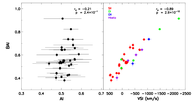
Figure 2.— Relation among the outflow indicators. Left panel: comparison of AI and BAI. Right panel: comparison of VSI versus BAI. The colors in right panel represent the reference lines for determining the systemic redshift ([S II]: red, [O I]: green, [O II]: blue, and H$\beta$: purple). Spearman’s rank correlation coefficients and their statistical significances are given in the top left side in each panel.

IV.1. Outflow indicators

As described in §3.1, the outflow indicators investigated in this work are AI, VSI, and BAI. The mean values and standard deviations for AI, VSI, and BAI are (0.51, 0.03), (–258 km s^-1, 566 km s^-1), and (0.57, 0.12), respectively. For comparison, the median value of those parameters given in Wang et al. (2011) for high-redshift QSOs are 0.5 (AI), -898 km s^-1 (VSI), and 0.63 (BAI). While the measured AI and BAI of our sample are similar to those of the high-redshift QSO sample of Wang et al. (2011), the VSI values of our sample are systematically smaller than those of Wang et al. (2011). The reason for this systematic difference may be owing to the difference in the sample selection (see §5.1).

To examine the reliability of the measured BAI and the relation between BAI and the other indicators (AI and VSI), we compare the three outflow indicators in Figure 2. The different colors of symbols in this figure denote different narrow lines used for determining the systemic redshift. We do not find any systematically different behaviors for different color symbols, suggesting that the difference in the narrow lines used for the redshift determination does not cause significant systematic effects in the outflow indicators. Therefore we combine all of the data obtained from different reference lines in the following analysis and discussion. Figure 2 shows that there is a clear correlation between BAI and VSI, while there is no apparent correlation between BAI and AI. To investigate whether or not there are statistically significant correlations among the outflow indices, we conduct Spearman’s rank-order correlation test with the null hypothesis that there are no correlations among the outflow indices. This null hypothesis is not rejected for the relation between BAI and AI ($p=2.4\times 10^{-1}$), while it is rejected for the relation between BAI and VSI with a high statistical significance ($p=2.9\times 10^{-12}$). This result is partly because the typical measurement uncertainty in AI is much larger than the standard deviation of the AI distribution (see the left panel in Figure 2). It is thus inferred that the AI parameter is not an adequate indicator for the AGN outflow, at least for our sample. Note that BAI and VSI are expected to show a correlation since both parameters are defined with velocity shift from the systematic velocity. Thus, it is not surprising to observe a correlation in Figure 2 (left).

IV.2. AGN properties and outflow

Here we investigate the relation between outflow indicators (BAI and VSI) and AGN properties. The mean values and standard deviations of $M_{\rm BH}/M_{{\odot}}$, $\lambda L_{5100}\ (\rm erg/s)$, and $L_{\rm Bol}/L_{\rm Edd}$ derived in §3.2 in logscale, are (8.20, 0.61), (45.23, 0.70), and (–1.07, 0.41), respectively. The bolometric luminosity of our sample is located at the bright part of the optical AGN luminosity function in the local universe (see, e.g., Boyle et al., 2000; Schulze et al., 2009). As for the Eddington ratio, our sample shows a wide range ($\sim$1.5 dex) in the Eddington ratio, distributed in the range of $-2.0\lesssim L_{\rm Bol}/L_{\rm Edd}\lesssim-0.5$. Thus our sample allows us to investigate the AGN outflow in a broad dynamic range of the Eddington ratio. Note that the Eddington ratio of the sample of Wang et al. (2011) distributes in the range of $-1.0\lesssim L_{\rm Bol}/L_{\rm Edd}\lesssim+0.5$, i.e., $\sim$1 dex higher than the Eddington ratio distribution of our sample. This difference is a natural consequence of the sample selection in the sense that high-redshift SDSS quasars are luminous enough to be selected in the magnitude-limited SDSS spectroscopy. The systematically smaller VSI in our sample than in the sample of Wang et al. (2011) mentioned in §4.1 is probably attributed by this $\sim$1 dex difference in the Eddington ratio distribution between the two samples.

In Figure 3, possible dependences of the two outflow indicators (BAI and VSI) on the AGN properties ($M_{\rm BH}$, $L_{\rm Bol}$, and $L_{\rm Bol}/L_{\rm Edd}$) are investigated. Note that the investigation of the relation between AI and those AGN properties is not useful, since the dynamic range of AI in our sample is too narrow (see §4.1 and Figure 2). Figure 3 shows that there is no apparent correlation between $M_{\rm BH}$ and outflow indicators. However in the center and right panel, the two outflow indicators appear to show positive correlations with the AGN bolometric luminosity and Eddington ratio, in the sense that AGNs with a higher luminosity or a higher Eddington ratio tend to show stronger outflows. For examining the statistical significance of these possible correlations, we conduct Spearman’s rank-order correlation test with the null hypothesis that there are no correlations in Figure 3. The rank-order test suggests that there is no correlation between the two outflow indicators (BAI and VSI) and $M_{\rm BH}$ ($p=1.6\times 10^{-1}$ and $p=1.3\times 10^{-1}$). It is also suggested that the inferred dependences of BAI and VSI on the AGN bolometric luminosity and Eddington ratio are marginal, but VSI shows more significant correlation with those two AGN parameters ($p=4.7\times 10^{-3}$ and $p=1.1\times 10^{-3}$) than BAI ($p=1.9\times 10^{-2}$ and $p=1.1\times 10^{-2}$). These trends are qualitatively consistent with the previous study for high-redshift QSOs reported by Wang et al. (2011).

Figure 3.— Comparison between the AGN properties ($M_{\rm BH}$, $L_{\rm bol}$, and $L_{\rm bol}/L_{\rm Edd}$) and the outflow indicators (BAI and VSI). The colors are the same as in Figure 2. Spearman’s rank correlation coefficients and their statistical significance are presented at the top-left side in each panel.

IV.3. Comparison between metallicity and outflow

The mean values and standard deviations of N V/C IV, (Si IV+O IV])/C IV, and N V/He IIderived in §3.3 in the logscale are (–0.41,0.29), (–0.65, 0.23), and (0.57, 0.22), respectively. As we mentioned in §3.3 the values are from Shin et al. (2013) and they are similar to those of previous works (e.g., Shemmer et al., 2004; Matsuoka et al., 2011).

Now we examine how the two outflow indicators (BAI and VSI) depend on the BLR metallicity. Figure 4 shows the comparison between the outflow indicators and BLR metallicity indicators. There are loose positive correlations in the sense that AGNs with a higher BLR metallicity tend to show stronger outflow, but the significance looks marginal. For examining the statistical significance of those possible correlations, we conduct Spearman’s rank-order correlation test with the null hypothesis that there are no correlations in Figure 4. The rank-order test suggests that the correlations between BAI and the metallicity indicators are very marginal with low statistical significance ($p\sim 0.01-0.17$). Though the statistical significances of correlations between VSI and the metallicity indicators are slightly higher ($p\sim 0.003-0.07$) than the correlations for BAI, but not very tight. These results seem contradictory to the earlier results for high redshift QSOs reported by Wang et al. (2012), who showed a tight correlation between the outflow strength and metallicity in BLRs. For this comparison, it should be noted that the analysis by Wang et al. (2012) is based on stacked SDSS spectra of 12844 high-redshift QSOs while our analysis is based on individual SDSS spectra of 34 low-redshift AGNs. A significantly larger number of objects in the study of Wang et al. (2012) makes the statistical error very small.

For investigating whether our results are consistent with those of Wang et al. (2012), we present the relation between BAI and (Si IV+O IV])/C IV high-redshift QSOs in Figure 4 (dashed line in the upper middle panel). Although the dispersion in our sample is large, the results of Wang et al. (2012) and ours show similar trend. This is interesting since the difference in the cosmic age between our sample at $z\sim 0.1$ and the sample of Wang et al. (2012) at $1.7<z<4$ is more than half of the Hubble time but still these two samples show a similar trend in the relation between the outflow indicator and metallicity indicator.

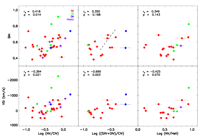
Figure 4.— Comparison between the metallicity indicators (N V/C IV, (Si IV+O IV])/C IV, and N V/He II) and the outflow indicators (BAI and VSI). The colors are the same as in Figure 2. Spearman’s rank correlation coefficients and their statistical significance are presented at the top-left side in each panel. The dashed line in the top-middle panel shows the previous result for high-redshift QSOs reported by Wang et al. (2012).

V. Discussion

V.1. Possible effects of the sample selection

As described in §4.2, the AI parameter does not work well for quantifying the outflow strength for our sample. This is attributed to the narrow range of the AI distribution. It is interesting to notice that highly asymmetric C IV lines are selectively seen in radio-loud QSOs (Sulentic et al., 2000, 2007). The small range of the AI distribution in our sample may be attributed to the fact that there are not so many radio-loud AGNs in the PG sample (Kellermann et al., 1989). Wang et al. (2011) reported a significant correlation between AI and BAI, based on their high-redshift SDSS QSO sample whose AI distributes in the range of $0.3\lesssim AI\lesssim 0.8$. However, the AI distribution of their sample concentrates mostly in the range of $0.4\lesssim AI\lesssim 0.6$, and actually the wide AI range is achieved owing to the large sample size. Therefore, the small sample size of ours (lacking radio-loud AGNs especially) is not adequate to investigate the AI distribution and various AI-related correlations. As for the BAI and VSI parameters, VSI shows tighter correlations with AGN properties including the BLR metallicity than BAI as shown in §4.2 and §4.3. This is possibly affected by the large uncertainty in AI that introduce the corresponding uncertainty in BAI.

Another potential concern for our sample selection is the removal of BAL AGNs. The BAL features are caused by powerful outflows of ionized gas, and thus possibly AGNs with a strong outflow may be selectively removed from our sample. This concern may not be true, if the fast ionized outflow is ubiquitous in AGNs and the BAL features are observed just due to the orientation effect (i.e., we see the BAL features only in $\sim$10% of type-1 AGNs because the covering factor of the ionized outflow is $\sim$10%; see, e.g., Weymann et al. 1991). It is interesting to compare the outflow indices (AI, VSI, and BAI) between BAL AGNs and non-BAL AGNs to understand the nature of the BAL phenomenon in AGNs; however we do not further discuss this issue because it is beyond the scope of this work.

V.2. Star formation and AGN activity

The correlations among the outflow, metallicity, and Eddington ratio seen in our sample suggest their physical connection in low-redshift AGNs. It suggests that the gas radial motion (i.e., the gas accretion onto the SMBH and the outflow from the nucleus) is related to the metallicity in the nuclear region. The relation between the metallicity and the gas accretion has been reported for QSOs (e.g., Shemmer et al., 2004), and also for nearby Seyfert galaxies especially focusing on the metallicity difference between narrow-line Seyfert 1 galaxies and broad-line Seyfert 1 galaxies (e.g., Nagao et al., 2002; Shemmer & Netzer, 2002; Fields et al., 2005). This can be interpreted as the result of the starburst-AGN connection; i.e., the nuclear starburst activity enriches the gas in the nuclear region and also triggers the gas accretion onto the SMBH. On the other hand, the relation between the AGN outflow and the Eddington ratio has been also discussed, in the sense that the gas accretion results in the increase of the AGN luminosity that causes the outward radiative pressure to the surrounding gas (e.g., Komossa et al., 2008; Wang et al., 2011; Marziani et al., 2013). Therefore the correlations among the outflow, metallicity, and Eddington ratio are reasonable characteristics in AGNs. In addition, a more direct reason causing the positive correlation between the gas metallicity and the outflow is that the gas with a high metallicity (and with a high dust abundance consequently) has a larger optical depth. Therefore such metal-rich clouds are more easily affected by the outward radiative pressure. Also, the resonant scattering could contribute to the outflow. If the resonant scattering exerts radiation pressure, higher metallicity gas has higher optical depth in the resonance scattering, that leads to more powerful outflow. Interestingly, our results for low-redshift ($z<0.4$) QSOs and those for high-redshift ($1.7<z<4$) QSOs show a similar trend, even though these two studies examine completely different cosmic epochs. This suggests that the physics of the gas accretion onto the SMBH and its relation to the nuclear star formation is universal through the cosmic timescale.

On the other hand, the SMBH mass does not show a significant correlation with the outflow. The correlation coefficients are 0.25 for low-redshift QSOs and -0.39 for high-redshift QSOs (Wang et al., 2011). This implies that the SMBH mass itself is not an important factor for nuclear activities such as nuclear star formation and outflow. This interpretation is consistent to the recent work by (Shin et al., 2013), reporting that there is no statistically meaningful correlation between the SMBH mass and the BLR metallicity.

V.3. OIII shift

The powerful AGN outflow is sometimes seen also in the NLR. Komossa et al. (2008) showed that the [O III] emission (a relatively high-ionization NLR line) in some AGNs shows a blue shift with respect to other low ionization narrow lines, such as [S II]. Since it is known that high-ionization NLR clouds (emitting [O III]) locate more inner parts in the NLR than low-ionization NLR clouds emitting such as [S II], [O I], and [O II] (Ferguson et al., 1997; Nagao et al., 2001), it is naturally expected that high-ionization NLR lines more frequently show outflow features than low-ionization NLR lines (e.g., Bae & Woo, 2014). Then a question naturally arises — is there any physical connection between BLR outflows and NLR outflows? In terms of the gas metallicity, some earlier works reported the physical connection between gas clouds in NLRs and BLRs (e.g., Fu & Stockton, 2007; Du et al., 2014). In these works, it is inferred that the outflowing BLR gas affects the chemical property in the NLR. Therefore, it is highly interesting to examine possible physical link between the BLR outflow and NLR outflow. This can be studied by investigating the outflow indices for C IV and those for [O III].

To investigate a possible link between the BLR outflow and NLR outflow, we focus on the outflow indices for [O III] and compare them with the outflow indices for C IV in our low-redshift AGN sample. Figure 5 shows the results of the comparison of VSI between [O III] and C IV. Here we derive the VSI by adopting different references for the systemic redshift; H$\beta$, [O I], [O II], and [S II], for checking the robustness of the inferred results. There is no apparent correlation between the VSI of [O III] and C IV, regardless of the adopted redshift reference. The Spearman’s rank-order correlation test also suggests that there is not statistically significant correlation between them (the exact results of the rank-order correlation test are given in Figure 5). However the obtained results do not necessarily mean that the BLR outflow and NLR outflow is independent, because the sample size of our low-redshift AGNs is so small that the covered range of the [O III] VSI is very limited (from –150 km s^-1 to +250 km s^-1 roughly). The studies of [O III] in the literature typically focus on the wing component, which represents the non-gravitational kinematic signature, finding evidence of strong outflows (Woo et al., 2016; Bae & Woo, 2016; Woo et al., 2017). On the other hand the velocity shift of [O III] is reported to be relatively small (Bae & Woo, 2014; Woo et al., 2016). Thus, our comparison of BLR and NLR outflows based on the velocity shift may not reveal a strong trend. The comparison of the outflow kinematics between [O III] and C IV for much larger samples with detailed line profile analysis will be an interesting test to understand a possible link between the BLR and NLR outflows.

Figure 5.— Comparison between [O III] and C IV VSIs. Each panel shows the comparison of them, adopting different narrow line for determining the systemic redshift (top left: H$\beta$, top right: [O I], bottom left: [O II], and bottom right: [S II]).

VI. Summary

To understand the AGN gas outflow at the BLR of low-redshift AGNs, we derive AGN outflow indicators of 34 low-redshift AGNs by analyzing the C IV velocity profile and by adopting the systemic redshift defined by some low-ionization narrow emission lines such as [S II] and [O I]. By comparing the measured outflow indicators with various AGN properties, the following results are obtained.

1. The outflow indicators (VSI and BAI of C IV) show weak positive correlations with the Eddington ratio, bolometric luminosity, and BLR metallicity indicators, suggesting that there is a connection among the past star formation, accretion, and AGN outflow in the nuclear region of host galaxies. However, there are little correlation between the BLR outflow indicators and the SMBH mass.

2. The inferred relation among the BLR metallicity, Eddington ratio, and BLR outflow, seen in our low-redshift AGN sample, is consistent with that seen in high-redshift QSO sample (Wang et al., 2011, 2012). This implies there is no significantly cosmological evolution of the mechanism triggering the AGN activity.

3. A possible relation between the BLR outflow and NLR outflow is also investigated, by comparing the outflow indicator (VSI) for C IV and [O III]. However, any apparent correlation between the two is not identified. This may be due to the small size of our sample, suggesting that more extensive studies based on larger samples are required.

References

- Abazajian et al. (2009) Abazajian, K. N., Adelman-McCarthy, J. K., Agüeros, M. A., et al. 2009, ApJS, 182, 543
- Bae & Woo (2014) Bae, H.-J., & Woo, J.-H. 2014, ApJ, 795, 30
- Bae & Woo (2016) Bae, H.-J., & Woo, J.-H. 2016, ApJ, 828, 97
- Baldwin et al. (1995) Baldwin, J., Ferland, G., Korista, K., & Verner, D. 1995, ApJ, 455, L119
- Baldwin et al. (2003) Baldwin, J. A., Ferland, G. J., Korista, K. T., Hamann, F., & Dietrich, M. 2003, ApJ, 582, 590
- Baskin & Laor (2005) Baskin, A., & Laor, A. 2005, MNRAS, 356, 1029
- Bauermeister et al. (2013) Bauermeister, A., Blitz, L., Bolatto, A., et al. 2013, ApJ, 768, 132
- Bennert et al. (2006a) Bennert, N., Jungwiert, B., Komossa, S., Haas, M., & Chini, R. 2006a, A&A, 459, 55
- Bennert et al. (2006b) —. 2006b, A&A, 456, 953
- Boyle et al. (2000) Boyle, B. J., Shanks, T., Croom, S. M., et al. 2000, MNRAS, 317, 1014
- Bruzual & Charlot (2003) Bruzual, G., & Charlot, S. 2003, MNRAS, 344, 1000
- Cappellari & Emsellem (2004) Cappellari, M., & Emsellem, E. 2004, PASP, 116, 138
- Cid Fernandes et al. (2001) Cid Fernandes, R., Heckman, T., Schmitt, H., González Delgado, R. M., & Storchi-Bergmann, T. 2001, ApJ, 558, 81
- Ciotti et al. (2010) Ciotti, L., Ostriker, J. P., & Proga, D. 2010, ApJ, 717, 708
- Clavel et al. (1991) Clavel, J., Reichert, G. A., Alloin, D., et al. 1991, ApJ, 366, 64
- Crenshaw et al. (2015) Crenshaw, D. M., Fischer, T. C., Kraemer, S. B., & Schmitt, H. R. 2015, ApJ, 799, 83
- Crenshaw et al. (2003) Crenshaw, D. M., Kraemer, S. B., & George, I. M. 2003, ARA&A, 41, 117
- Croton et al. (2006) Croton, D. J., Springel, V., White, S. D. M., et al. 2006, MNRAS, 365, 11
- Daddi et al. (2010) Daddi, E., Bournaud, F., Walter, F., et al. 2010, ApJ, 713, 686
- Di Matteo et al. (2005) Di Matteo, T., Springel, V., & Hernquist, L. 2005, Nature, 433, 604
- Du et al. (2014) Du, P., Wang, J.-M., Hu, C., et al. 2014, MNRAS, 438, 2828
- Ferguson et al. (1997) Ferguson, J. W., Korista, K. T., Baldwin, J. A., & Ferland, G. J. 1997, ApJ, 487, 122
- Ferrarese & Merritt (2000) Ferrarese, L., & Merritt, D. 2000, ApJ, 539, L9
- Fields et al. (2005) Fields, D. L., Mathur, S., Pogge, R. W., Nicastro, F., & Komossa, S. 2005, ApJ, 620, 183
- Fraquelli et al. (2003) Fraquelli, H. A., Storchi-Bergmann, T., & Levenson, N. A. 2003, MNRAS, 341, 449
- Fu & Stockton (2007) Fu, H., & Stockton, A. 2007, ApJ, 664, L75
- Gaibler et al. (2012) Gaibler, V., Khochfar, S., Krause, M., & Silk, J. 2012, MNRAS, 425, 438
- Ganguly et al. (2007) Ganguly, R., Brotherton, M. S., Cales, S., et al. 2007, ApJ, 665, 990
- García-Burillo et al. (2014) García-Burillo, S., Combes, F., Usero, A., et al. 2014, A&A, 567, A125
- Gaskell (1982) Gaskell, C. M. 1982, ApJ, 263, 79
- Geach et al. (2011) Geach, J. E., Smail, I., Moran, S. M., et al. 2011, ApJ, 730, L19
- Gebhardt et al. (2000) Gebhardt, K., Bender, R., Bower, G., et al. 2000, ApJ, 539, L13
- Granato et al. (2004) Granato, G. L., De Zotti, G., Silva, L., Bressan, A., & Danese, L. 2004, ApJ, 600, 580
- Hamann & Ferland (1999) Hamann, F., & Ferland, G. 1999, ARA&A, 37, 487
- Häring & Rix (2004) Häring, N., & Rix, H.-W. 2004, ApJ, 604, L89
- Harris et al. (2012) Harris, C. E., Bennert, V. N., Auger, M. W., et al. 2012, ApJS, 201, 29
- Harrison et al. (2014) Harrison, C. M., Alexander, D. M., Mullaney, J. R., & Swinbank, A. M. 2014, MNRAS, 441, 3306
- Heckman et al. (1997) Heckman, T. M., González-Delgado, R., Leitherer, C., et al. 1997, ApJ, 482, 114
- Hewett & Wild (2010) Hewett, P. C., & Wild, V. 2010, MNRAS, 405, 2302
- Hopkins et al. (2006) Hopkins, P. F., Hernquist, L., Cox, T. J., et al. 2006, ApJS, 163, 1
- Husemann et al. (2016) Husemann, B., Scharwächter, J., Bennert, V. N., et al. 2016, A&A, 594, A44
- Ishibashi et al. (2013) Ishibashi, W., Fabian, A. C., & Canning, R. E. A. 2013, MNRAS, 431, 2350
- Juarez et al. (2009) Juarez, Y., Maiolino, R., Mujica, R., et al. 2009, A&A, 494, L25
- Karouzos et al. (2016) Karouzos, M., Woo, J.-H., & Bae, H.-J. 2016, ApJ, 819, 148
- Kaspi et al. (2000) Kaspi, S., Smith, P. S., Netzer, H., et al. 2000, ApJ, 533, 631
- Kauffmann & Haehnelt (2000) Kauffmann, G., & Haehnelt, M. 2000, MNRAS, 311, 576
- Kellermann et al. (1989) Kellermann, K. I., Sramek, R., Schmidt, M., Shaffer, D. B., & Green, R. 1989, AJ, 98, 1195
- Komossa et al. (2008) Komossa, S., Xu, D., Zhou, H., Storchi-Bergmann, T., & Binette, L. 2008, ApJ, 680, 926
- Korista & Goad (2000) Korista, K. T., & Goad, M. R. 2000, ApJ, 536, 284
- Kormendy & Ho (2013) Kormendy, J., & Ho, L. C. 2013, ARA&A, 51, 511
- Magorrian et al. (1998) Magorrian, J., Tremaine, S., Richstone, D., et al. 1998, AJ, 115, 2285
- Maiolino et al. (2012) Maiolino, R., Gallerani, S., Neri, R., et al. 2012, MNRAS, 425, L66
- Marconi & Hunt (2003) Marconi, A., & Hunt, L. K. 2003, ApJ, 589, L21
- Marziani et al. (1996) Marziani, P., Sulentic, J. W., Dultzin-Hacyan, D., Calvani, M., & Moles, M. 1996, ApJS, 104, 37
- Marziani et al. (2013) Marziani, P., Sulentic, J. W., Plauchu-Frayn, I., & del Olmo, A. 2013, ApJ, 764, 150
- Matsuoka et al. (2011) Matsuoka, K., Nagao, T., Marconi, A., Maiolino, R., & Taniguchi, Y. 2011, A&A, 527, A100
- Matsuoka & Woo (2015) Matsuoka, K., & Woo, J.-H. 2015, ApJ, 807, 28
- McIntosh et al. (1999) McIntosh, D. H., Rix, H.-W., Rieke, M. J., & Foltz, C. B. 1999, ApJ, 517, L73
- Merloni et al. (2004) Merloni, A., Rudnick, G., & Di Matteo, T. 2004, MNRAS, 354, L37
- Müller-Sánchez et al. (2011) Müller-Sánchez, F., Prieto, M. A., Hicks, E. K. S., et al. 2011, ApJ, 739, 69
- Nagao et al. (2006) Nagao, T., Marconi, A., & Maiolino, R. 2006, A&A, 447, 157
- Nagao et al. (2002) Nagao, T., Murayama, T., Shioya, Y., & Taniguchi, Y. 2002, ApJ, 575, 721
- Nagao et al. (2001) Nagao, T., Murayama, T., & Taniguchi, Y. 2001, ApJ, 549, 155
- Nagao et al. (2000) Nagao, T., Taniguchi, Y., & Murayama, T. 2000, AJ, 119, 2605
- Netzer (2009) Netzer, H. 2009, MNRAS, 399, 1907
- Park et al. (2012a) Park, D., Kelly, B. C., Woo, J.-H., & Treu, T. 2012a, ApJS, 203, 6
- Park et al. (2015) Park, D., Woo, J.-H., Bennert, V. N., et al. 2015, ApJ, 799, 164
- Park et al. (2012b) Park, D., Woo, J.-H., Treu, T., et al. 2012b, ApJ, 747, 30
- Popping et al. (2015) Popping, G., Caputi, K. I., Trager, S. C., et al. 2015, MNRAS, 454, 2258
- Richards et al. (2002) Richards, G. T., Vanden Berk, D. E., Reichard, T. A., et al. 2002, AJ, 124, 1
- Scannapieco et al. (2012) Scannapieco, C., Wadepuhl, M., Parry, O. H., et al. 2012, MNRAS, 423, 1726
- Schulze & Wisotzki (2010) Schulze, A., & Wisotzki, L. 2010, A&A, 516, A87
- Schulze et al. (2009) Schulze, A., Wisotzki, L., & Husemann, B. 2009, A&A, 507, 781
- Shemmer & Netzer (2002) Shemmer, O., & Netzer, H. 2002, ApJ, 567, L19
- Shemmer et al. (2004) Shemmer, O., Netzer, H., Maiolino, R., et al. 2004, ApJ, 614, 547
- Shin et al. (2013) Shin, J., Woo, J.-H., Nagao, T., & Kim, S. C. 2013, ApJ, 763, 58
- Silk (2005) Silk, J. 2005, MNRAS, 364, 1337
- Sulentic et al. (2007) Sulentic, J. W., Bachev, R., Marziani, P., Negrete, C. A., & Dultzin, D. 2007, ApJ, 666, 757
- Sulentic et al. (2000) Sulentic, J. W., Marziani, P., & Dultzin-Hacyan, D. 2000, ARA&A, 38, 521
- Tacconi et al. (2010) Tacconi, L. J., Genzel, R., Neri, R., et al. 2010, Nature, 463, 781
- Tacconi et al. (2013) Tacconi, L. J., Neri, R., Genzel, R., et al. 2013, ApJ, 768, 74
- Tombesi et al. (2012) Tombesi, F., Cappi, M., Reeves, J. N., & Braito, V. 2012, MNRAS, 422, L1
- Trakhtenbrot & Netzer (2012) Trakhtenbrot, B., & Netzer, H. 2012, MNRAS, 427, 3081
- Tsuzuki et al. (2006) Tsuzuki, Y., Kawara, K., Yoshii, Y., et al. 2006, ApJ, 650, 57
- Vanden Berk et al. (2001) Vanden Berk, D. E., Richards, G. T., Bauer, A., et al. 2001, AJ, 122, 549
- Véron-Cetty & Véron (2010) Véron-Cetty, M.-P., & Véron, P. 2010, A&A, 518, A10
- Vestergaard et al. (2008) Vestergaard, M., Fan, X., Tremonti, C. A., Osmer, P. S., & Richards, G. T. 2008, ApJ, 674, L1
- Wang et al. (2011) Wang, H., Wang, T., Zhou, H., et al. 2011, ApJ, 738, 85
- Wang et al. (2012) Wang, H., Zhou, H., Yuan, W., & Wang, T. 2012, ApJ, 751, L23
- Weymann et al. (1991) Weymann, R. J., Morris, S. L., Foltz, C. B., & Hewett, P. C. 1991, ApJ, 373, 23
- Wilkes (1984) Wilkes, B. J. 1984, MNRAS, 207, 73
- Woo et al. (2017) Woo, J.-H., Son, D., & Bae, H.-J., 2017, ApJ, submitted
- Woo et al. (2016) Woo, J.-H., Bae, H.-J., Son, D., & Karouzos, M. 2016, ApJ, 817, 108
- Woo et al. (2012) Woo, J.-H., Kim, J. H., Imanishi, M., & Park, D. 2012, AJ, 143, 49
- Woo et al. (2013) Woo, J.-H., Schulze, A., Park, D., et al. 2013, ApJ, 772, 49
- Woo et al. (2008) Woo, J.-H., Treu, T., Malkan, M. A., & Blandford, R. D. 2008, ApJ, 681, 925
- Woo et al. (2015) Woo, J.-H., Yoon, Y., Park, S., Park, D., & Kim, S. C. 2015, ApJ, 801, 38
- Wu et al. (2015) Wu, X.-B., Wang, F., Fan, X., et al. 2015, Nature, 518, 512
- York et al. (2000) York, D. G., Adelman, J., Anderson, Jr., J. E., et al. 2000, AJ, 120, 1579
- Zhang et al. (2013) Zhang, K., Wang, T.-G., Yan, L., & Dong, X.-B. 2013, ApJ, 768, 22
- Zubovas et al. (2013) Zubovas, K., Nayakshin, S., King, A., & Wilkinson, M. 2013, MNRAS, 433, 3079