Species with potential arising from surfaces with orbifold points of order 2, Part II: arbitrary weights

Abstract.

Let ${\mathbf{\Sigma}}=(\Sigma,\mathbb{M},\mathbb{O})$ be either an unpunctured surface with marked points and order-2 orbifold points, or a once-punctured closed surface with order-2 orbifold points. For each pair $(\tau,\omega)$ consisting of a triangulation $\tau$ of ${\mathbf{\Sigma}}$ and a function $\omega:\mathbb{O}\rightarrow\{1,4\}$, we define a chain complex ${C_{\bullet}({\tau,\omega})}$ with coefficients in $\mathbb{F}_{2}=\mathbb{Z}/2\mathbb{Z}$. Given ${\mathbf{\Sigma}}$ and $\omega$, we define a colored triangulation of ${\mathbf{\Sigma}_{\omega}}=(\Sigma,\mathbb{M},\mathbb{O},\omega)$ to be a pair $(\tau,\xi)$ consisting of a triangulation of ${\mathbf{\Sigma}}$ and a 1-cocycle in the cochain complex which is dual to ${C_{\bullet}({\tau,\omega})}$; the combinatorial notion of colored flip of colored triangulations is then defined as a refinement of the notion of flip of triangulations. Our main construction associates to each colored triangulation a species and a potential, and our main result shows that colored triangulations related by a flip have species with potentials (SPs) related by the corresponding SP-mutation as defined in [27].

We define the flip graph of colored triangulations of ${\mathbf{\Sigma}_{\omega}}$ as the graph whose vertices are the pairs $(\tau,x)$ consisting of a triangulation $\tau$ and a cohomology class $x\in{H^{1}(C^{\bullet}({\tau,\omega}))}$, with an edge connecting two such pairs $(\tau,x)$ and $(\sigma,z)$ if and only if there exist 1-cocycles $\xi\in x$ and $\zeta\in z$ such that $(\tau,\xi)$ and $(\sigma,\zeta)$ are colored triangulations related by a colored flip; then we prove that this flip graph is always disconnected provided the underlying surface $\Sigma$ is not contractible.

In the absence of punctures, we show that the Jacobian algebras of the SPs constructed are finite-dimensional and that whenever two colored triangulations have the same underlying triangulation, the Jacobian algebras of their associated SPs are isomorphic if and only if the underlying 1-cocycles have the same cohomology class; we also give a full classification of the non-degenerate SPs one can associate to any given pair $(\tau,\omega)$ over cyclic Galois extensions with primitive $4^{\operatorname{th}}$ roots of unity.

The species constructed here are species realizations of the $2^{|\mathbb{O}|}$ skew-symmetrizable matrices that Felikson-Shapiro-Tumarkin associated in [18] to any given triangulation of ${\mathbf{\Sigma}}$. In the prequel [27] to this paper we constructed a species realization of only one of these matrices, but therein we allowed the presence of arbitrarily many punctures.

1. Introduction

In [18], Felikson-Shapiro-Tumarkin showed how $2^{|\mathbb{O}|}$ different cluster algebras can be associated to a surface with marked points and order-2 orbifold points ${\mathbf{\Sigma}}=(\Sigma,\mathbb{M},\mathbb{O})$. They did so by assigning $2^{|\mathbb{O}|}$ skew-symmetrizable matrices to each (tagged) triangulation of ${\mathbf{\Sigma}}$, and by showing that if two (tagged) triangulations are related by a flip, then the two assigned $2^{|\mathbb{O}|}$-tuples of matrices are related by the corresponding matrix mutation of Fomin-Zelevinsky. They then used the alluded $2^{|\mathbb{O}|}$ cluster algebras to study the “lambda length coordinate ring” of the corresponding decorated Teichmüller space in a way similar to the one established by Fomin-Shapiro-Thurston [20] and Fomin-Thurston in [21] in the case of surfaces with marked points and without orbifold points.

In [27] we associated a species and a potential to each triangulation of a possibly punctured surface with marked points and order-2 orbifold points, and proved that triangulations related by a flip have species with potential related by the SP-mutation also defined in [27]. The species constructed therein for any given triangulation $\tau$ is a species realization of only one of the $2^{|\mathbb{O}|}$ skew-symmetrizable matrices assigned by Felikson-Shapiro-Tumarkin to $\tau$. In this paper we consider surfaces that are either unpunctured with order-2 orbifold points, or once-punctured closed with order-2 orbifold points, and for every ideal triangulation of such surfaces we realize the $2^{|\mathbb{O}|}$ matrices of Felikson-Shapiro-Tumarkin via SPs. Our main result, Theorem 7.1, asserts that the SP-mutations of the SPs we construct are compatible with the flips of triangulations. More precisely, we introduce the notions of colored triangulation and colored flip, which are refinements of the notions of ideal triangulation and flip, associate an SP to each colored triangulation, and show that whenever two colored triangulations are related by a colored flip, then the associated SPs are related by the corresponding SP-mutation defined in [27].

Let us say some words about the context within which this paper has been written; this context dates back at least ten years, to the works of Derksen-Weyman-Zelevinsky [14] and Fomin-Shapiro-Thurston [20], which themselves go back to the turn-of-the-century discovery and invention by Sergey Fomin and Andrei Zelevinsky of nowadays pervasive cluster algebras [22].

The mutation theory of quivers with potential developed by Derksen-Weyman-Zelevinsky in [14] has turned out to be very useful both inside and outside cluster-algebra theory. In cluster algebras, it provided representation-theoretic means for solutions, in the case of skew-symmetric cluster algebras, of several conjectures stated by Fomin-Zelevinsky in [24] (see, for instance, [15] and [10]). Outside cluster algebras, one of the reasons of its usefulness is that, thanks to a powerful result of Keller-Yang [28], it can be thought of as a down-to-earth counterpart of tilting in certain triangulated categories.

Motivated by [14] and by Fomin-Shapiro-Thurston’s assignment of a signed-adjacency quiver to every tagged triangulation of a surface with marked points and without orbifold points (cf. [20]) and by the compatibility between flips and quiver mutations this assignment possesses, the second author of the present paper noticed in [30] and [31] that every tagged triangulation of a surface with marked points and without orbifold points comes with a “natural” potential on its signed-adjacency quiver, and proved that if two tagged triangulations are related by a flip, then the associated quivers with potential are related by the corresponding QP-mutation of Derksen-Weyman-Zelevinsky. A combination of this result with the result of Keller-Yang referred to above allows to associate to any surface with marked points and without orbifold points a 3-Calabi-Yau triangulated category, the combinatorics of whose “canonical” hearts and tilts is parametrized and governed by the tagged triangulations of the surface and the flips of triangulations. Similarly, combining the results of [30, 31] with the constructions and results given by Amiot in [1, 2] allows to associate to the surface a 2-Calabi-Yau Hom-finite triangulated category whose “canonical” cluster-tilting objects are parametrized by tagged triangulations, and with the IY-mutation of cluster-tilting objects modeled by the combinatorial operation of flip of arcs in triangulations. The present paper has been written in the belief and hope that similar associations of triangulated categories to surfaces with marked points and order-2 orbifold points can be made and that, this way, the SPs constructed here can turn out to be as useful as the QPs associated to triangulations of surfaces without orbifold points have turned out to be.

Now, we describe the contents of the paper in more detail. In Section 2 we recall the framework of surfaces with marked points and order-2 orbifold points, to which Felikson-Shapiro-Tumarkin have associated several cluster algebras in [18]. The framework we recall is less general than Felikson-Shapiro-Tumarkin’s framework since we will work only with surfaces that either are unpunctured (with an arbitrary number of orbifold points) or once-punctured with empty boundary (again with arbitrarily many orbifold points).

Letting ${\mathbf{\Sigma}}=(\Sigma,\mathbb{M},\mathbb{O})$ be any surface as in the previous paragraph, in Section 3 we describe the $2^{|\mathbb{O}|}$ weighted quivers (that correspond under [32, Lemma 2.3] to the $2^{|\mathbb{O}|}$ skew-symmetrizable matrices) associated by Felikson-Shapiro-Tumarkin to any given triangulation $\tau$ of $(\Sigma,\mathbb{M},\mathbb{O})$. More precisely, we describe a rule that for each pair $(\tau,\omega)$ consisting of a triangulation $\tau$ of $(\Sigma,\mathbb{M},\mathbb{O})$ and a function $\omega:\mathbb{O}\rightarrow\{1,4\}$ allows us to obtain a weighted quiver $(Q(\tau,\omega),\mathbf{d}(\tau,\omega))$, where $Q(\tau,\omega)$ is defined in terms of the signed adjacencies between the arcs in $\tau$ (and also takes the function $\omega$ into account), and the tuple $\mathbf{d}(\tau,\omega)$ is defined so as to attach the integer $2$ to every arc not containing any orbifold point, and the integer $\omega(q)$ to each arc containing an orbifold point $q\in\mathbb{O}$. For a fixed $\tau$, the functions $\omega:\mathbb{O}\rightarrow\{1,4\}$, parametrize all the weighted quivers that correspond under [32, Lemma 2.3] to the $2^{|\mathbb{O}|}$ skew-symmetrizable matrices attached to $\tau$ by Felikson-Shapiro-Tumarkin. In Section 3 we also define two auxiliary quivers $Q^{\prime}(\tau,\omega)$ and $Q^{\prime\prime}(\tau,\omega)$, which we use in Section 4 to define two chain complexes $C_{\bullet}(\tau,\omega)$ and $\widehat{C}_{\bullet}(\tau,\omega)$ with coefficients in the field $\mathbb{F}_{2}=\mathbb{Z}/2\mathbb{Z}$ for each fixed pair $(\tau,\omega)$.

Let us stress at this point that, starting in Section 3 and to the very end of the paper, we will work not only with a fixed surface ${\mathbf{\Sigma}}=(\Sigma,\mathbb{M},\mathbb{O})$, but also with a fixed function $\omega:\mathbb{O}\rightarrow\{1,4\}$; only the triangulations will be allowed to vary from Section 3 to the end of the paper.

Just as a quiver alone does not suffice to define a path algebra, for the further specification of a ground field is necessary, having a weighted quiver is not enough to define a path algebra, for the further specifications of an appropriate ground field extension and of a modulating function are needed (see [27, Subsection 2.4 and Section 3.1 up to Definition 3.5]). So, besides the weighted quiver $(Q(\tau,\omega),\mathbf{d}(\tau,\omega))$, we need an appropriate field extension and a modulating function in order to be able to associate a species and a (complete) path algebra to $(Q(\tau,\omega),\mathbf{d}(\tau,\omega))$. In Section 4 we define a chain complex $C_{\bullet}(\tau,\omega)$ in terms of the quiver $Q^{\prime}(\tau,\omega)$ and of the triangles of the triangulation $\tau$; each choice of an element of the first cocycle group of the cochain complex which is $\mathbb{F}_{2}$-dual to $C_{\bullet}(\tau,\omega)$ will allow us to read off a modulating function for $(Q(\tau,\omega),\mathbf{d}(\tau,\omega))$ whenever we are given a degree-$d$ cyclic Galois field extension $E/F$, with $F$ having primitive $d^{\operatorname{th}}$ roots of unity, where $d=\operatorname{lcm}(\mathbf{d}(\tau,\omega))\in\{2,4\}$. This means, in particular, that we will attach not only one species to a given pair $(\tau,\omega)$ even when the field extension $E/F$ is fixed, but as many as 1-cocycles the cochain complex $C^{\bullet}(\tau,\omega):=\operatorname{Hom}_{\mathbb{F}_{2}}(C_{\bullet}(\tau,\omega),\mathbb{F}_{2})$ has. Let $Z^{1}(\tau,\omega)$ be the $\mathbb{F}_{2}$-vector subspace of $C^{1}(\tau,\omega):=\operatorname{Hom}_{\mathbb{F}_{2}}(C_{1}(\tau,\omega),\mathbb{F}_{2})$ whose elements are such 1-cocycles. In order to be able to define the combinatorial operation of flip of a pair $(\tau,\xi)$ consisting of a triangulation $\tau$ and a 1-cocycle $\xi\in Z^{1}(\tau,\omega)$, in Section 4 we use the quiver $Q^{\prime\prime}(\tau,\omega)$ to define an auxiliary chain complex $\widehat{C}_{\bullet}(\tau,\omega)$ whose $\mathbb{F}_{2}$-dual cochain complex will help us to define the desired notion of flip of $(\tau,\xi)$ with respect to an arc of $\tau$.

In Section 5 we introduce the notions of colored triangulations and their flips, which we distinguish from the flips of ordinary triangulations by calling them colored flips. Given a fixed ${\mathbf{\Sigma}_{\omega}}=(\Sigma,\mathbb{M},\mathbb{O},\omega)$, a colored triangulation of ${\mathbf{\Sigma}_{\omega}}$ is defined to be any pair $(\tau,\xi)$ consisting of a triangulation $\tau$ of ${\mathbf{\Sigma}}$ and a 1-cocycle $\xi\in{Z^{1}({\tau,\omega})}\subseteq C^{1}(\tau,\omega)$. The colored flip of a colored triangulation $(\tau,\xi)$ with respect to an arc $k\in\tau$ is defined in Section 5 as well and produces another colored triangulation $(\sigma,\zeta)=f_{k}(\tau,\xi)$, with $\sigma$ defined to be the triangulation obtained by applying the ordinary flip of $k$ to $\tau$, and $\zeta$ defined to be a certain 1-cocycle inside the cochain complex $C^{1}(\sigma,\omega)$, see Definition 5.8. The assignment $\xi\mapsto\zeta$ does not always constitute a group homomorphism ${Z^{1}({\tau,\omega})}\rightarrow Z^{1}(\sigma,\omega)$, and is defined after passing to the larger auxiliary cochain complexes $\widehat{C}^{\bullet}(\tau,\omega)=\operatorname{Hom}_{\mathbb{F}_{2}}(\widehat{C}_{\bullet}(\tau,\omega),\mathbb{F}_{2})$ and $\widehat{C}^{\bullet}(\sigma,\omega)=\operatorname{Hom}_{\mathbb{F}_{2}}(\widehat{C}_{\bullet}(\sigma,\omega),\mathbb{F}_{2})$.

Section 6 is devoted to associating to each colored triangulation $(\tau,\xi)$ an SP over any degree-$d$ cyclic Galois field extension $E/F$ with the property that $F$ has a primitive $d^{\operatorname{th}}$ root of unity, where $d=\operatorname{lcm}(\mathbf{d}(\tau,\omega))\in\{2,4\}$. Given such an extension $E/F$ and a colored triangulation $(\tau,\xi)$ of our fixed ${\mathbf{\Sigma}_{\omega}}$, in Subsection 6.1 we attach to each $k\in\tau$ the unique subfield $F_{k}$ of $E$ such that $[F_{k}:F]=d(\tau,\omega)_{k}$, and show how the 1-cocycle $\xi\in Z^{1}(\tau,\omega)\subseteq C^{1}(\tau,\omega)$ naturally gives rise to a modulating function $g(\tau,\xi):Q(\tau,\omega)_{1}\rightarrow\bigcup_{j,k\in\tau}\operatorname{Gal}(F_{j}\cap F_{k}/F)$ and hence to a species $A(\tau,\xi)$. In Subsection 6.2 we locate some ‘obvious’ cycles on $A(\tau,\xi)$ for the different types of triangles that $\tau$ can have, and define a potential $S(\tau,\xi)\in R\langle\langle A(\tau,\xi)\rangle\rangle$ as the sum of such ‘obvious’ cycles. The definition of $S(\tau,\xi)$ follows the same basic idea of [30], [31] and [27] in that it is the sum of cyclic paths on $A(\tau,\xi)$ that are ‘as obvious as possible’.

In Section 7 we arrive at Theorem 7.1, the main result of this paper, stated for surfaces that are either unpunctured with order-2 orbifold points, or once-punctured closed with order-2 orbifold points: for such a surface ${\mathbf{\Sigma}}=(\Sigma,\mathbb{M},\mathbb{O})$ and any fixed function $\omega:\mathbb{O}\rightarrow\{1,4\}$, if $(\tau,\xi)$ and $(\sigma,\zeta)$ are colored triangulations of ${\mathbf{\Sigma}_{\omega}}=(\Sigma,\mathbb{M},\mathbb{O},\omega)$ that are related by the colored flip of an arc $k\in\tau$, then the associated SPs $(A(\tau,\xi),S(\tau,\xi))$ and $(A(\sigma,\zeta),S(\sigma,\zeta))$ are related by the $k^{\operatorname{th}}$ SP-mutation defined in [27]. More precisely, the SPs $\mu_{k}(A(\tau,\xi),S(\tau,\xi))$ and $(A(\sigma,\zeta),S(\sigma,\zeta))$ are right-equivalent, where $\mu_{k}(A(\tau,\xi),S(\tau,\xi))$ is obtained from $(A(\tau,\xi),S(\tau,\xi))$ by applying [27, Definitions 3.19 and 3.22]. Consisting of a careful and detailed case-by-case analysis of the possible configurations that $\tau$ and $\omega$ can present around the arc $k$, the proof of Theorem 7.1 is rather lengthy and hence deferred to Section 14.

In Section 8 we show that the homology groups of the chain complex $C_{\bullet}(\tau,\omega)$ (resp. $\widehat{C}_{\bullet}(\tau,\omega)$) and the cohomology groups of its dual chain complex $C^{\bullet}(\tau,\omega)$ (resp. $\widehat{C}^{\bullet}(\tau,\omega)$) are respectively isomorphic to the singular homology and cohomology groups with coefficients in $\mathbb{F}_{2}$ of a surface $\widetilde{\Sigma}$ (resp. $\widehat{\Sigma}$) which is closely related to $\Sigma$. These isomorphisms will turn out to be canonical in the sense that for any two triangulations $\tau$ and $\sigma$ of ${\mathbf{\Sigma}}$ that are related by the flip of an arc $k\in\tau$ we will have several commutative diagrams, the most important one being the diagram

(see Proposition 8.9). The desired canonical isomorphisms are obtained by giving concrete “geometric realizations” of the complexes $C^{\bullet}(\tau,\omega)$ (resp. $\widehat{C}^{\bullet}(\tau,\omega)$); more precisely, by realizing these complexes as cellular complexes with coefficients in $\mathbb{F}_{2}$ of some very concrete topological subspaces $Y(\tau,\omega)\subseteq\widehat{Y}(\tau,\omega)$ of $\Sigma$.

In Section 9 we define two different flip graphs for a given ${\mathbf{\Sigma}_{\omega}}$. The cocycle flip graph is the graph that has the colored triangulations of ${\mathbf{\Sigma}_{\omega}}$ as its vertices, with an edge joining two colored triangulations precisely if they are related by a colored flip. The flip graph is the simple graph obtained from the cocycle flip graph by identifying two vertices $(\tau,\xi)$ and $(\tau^{\prime},\xi^{\prime})$ precisely when $\tau=\tau^{\prime}$ and $[\xi]=[\xi^{\prime}]$ as elements of $H^{1}(C^{\bullet}(\tau,\omega))$. With the aid of the isomorphisms from Section 8, we show that both of these graphs are disconnected if $\Sigma$ happens to be not contractible as a topological space.

Section 10 is devoted to showing that if we are given colored triangulations $(\tau,\xi)$ and $(\tau,\xi^{\prime})$ with the same underlying triangulation, then the corresponding Jacobian algebras $\mathcal{P}(A(\tau,\xi),S(\tau,\xi))$ and $\mathcal{P}(A(\tau,\xi^{\prime}),S(\tau,\xi^{\prime}))$ are isomorphic as rings through an $F$-algebra isomorphism that fixes each of the basic idempotents if and only if the 1-cocycles $\xi$ and $\xi^{\prime}$ have the same cohomology class in $H^{1}(C^{\bullet}(\tau,\omega))$. Consequently, for a fixed $(\tau,\omega)$ the (isomorphism classes of the) Jacobian algebras we construct for colored triangulations of $(\tau,\omega)$ are bijectively parametrized by the first cohomology group $H^{1}(C^{\bullet}(\tau,\omega))$, see Theorem 10.1.

In Section 11 we classify all possible realizations that the skew-symmetrizable matrices $B(\tau,\omega)$ can have via non-degenerate SPs up to right-equivalence. More precisely, we show that if ${\mathbf{\Sigma}}$ is an unpunctured surface different from a once-marked torus without orbifold points, $(\tau,\omega)$ is any pair consisting of a triangulation $\tau$ of ${\mathbf{\Sigma}}$ and a function $\omega:\mathbb{O}\rightarrow\{1,4\}$, $A$ is a species realization of $B(\tau,\omega)$ over $E/F$ (where as before $E/F$ is a degree-$d$ cyclic Galois field extension with $d=\operatorname{lcm}(\mathbf{d}(\tau,\omega))$) that admits a non-degenerate potential $S$ (in the sense of Derksen-Weyman-Zelevinsky), then there exists a 1-cocycle $\xi\in Z^{1}(\tau,\omega)\subseteq C^{1}(\tau,\omega)$ such that the SP $(A,S)$ is right-equivalent to the SP $(A(\tau,\xi),S(\tau,\xi))$.

Taking into account what we have said in the third, fourth and fifth paragraphs of this introduction, in Section 12 we state some problems and questions that, in our opinion, arise naturally from the constructions and results of this paper. For instance, we believe that if ${\mathbf{\Sigma}}$ is an unpunctured disc with at most two orbifold points, then for any $\omega:\mathbb{O}\rightarrow\{1,4\}$ and any colored triangulation $(\tau,\xi)$ of ${\mathbf{\Sigma}_{\omega}}$ the resulting Jacobian algebra $\mathcal{P}(A(\tau,\xi),S(\tau,\xi))$ is a cluster-tilted algebra in the sense [8, 9] of Buan-Marsh-Reineke-Reiten-Todorov and Buan-Marsh-Reiten. We also wonder whether the constructions and results of Amiot [1, 2], Keller-Yang [28] and Plamondon [36, 37] can be applied as are or adapted in order to associate 2- and 3-Calabi-Yau triangulated categories to ${\mathbf{\Sigma}_{\omega}}$ via the SPs we have constructed in this paper. We ask whether our constructions of SPs can be generalized so as to encompass all arbitrarily punctured surfaces with order-2 orbifold points.

Section 13 is devoted to discussing how the matrices that are mutation-equivalent to a matrix of Dynkin type $\mathbb{A}_{n}$, $\mathbb{C}_{n}$ or $\mathbb{B}_{n}$, or of affine type $\widetilde{\mathbb{C}}_{n}$, $\widetilde{\mathbb{B}}_{n}$, or $\widetilde{\mathbb{BC}}_{n}$, can be realized by SPs associated to colored triangulations of polygons with at most two orbifold points. We also point out that, over the complex numbers, our constructions associate two non-Morita-equivalent path algebras to the Kronecker quiver, one of them being the well known path algebra on which $\mathbb{C}$ acts centrally. Finally, we briefly outline the relation that the constructions and results of this paper keep with those given previously by Assem-Brüstle-Charbonneau-Plamondon [6], by those who this write [27] and by the second author of the present paper [30, 31].

Section 14 closes the paper with a case-by-case proof of Theorem 7.1, which, as we have said above, is the main result of this work.

2. Triangulated surfaces with weighted orbifold points

Recall from [27, Definition 2.1] that a surface with marked points and orbifold points of order $2$ is a triple ${\mathbf{\Sigma}}=(\Sigma,\mathbb{M},\mathbb{O})$ where

• $\Sigma$ is an oriented connected compact real surface with boundary $\partial\Sigma$,

• $\mathbb{M}\subseteq\Sigma$ is a non-empty finite set meeting each connected component of $\partial\Sigma$ at least once,

• $\mathbb{O}\subseteq\Sigma\setminus(\partial\Sigma\cup\mathbb{M})$ is a finite set (possibly empty).

The elements in $\mathbb{M}$ are called marked points and those in $\mathbb{O}$ orbifold points of order $2$. Marked points belonging to the interior $\Sigma\setminus\partial\Sigma$ are known as punctures. We shall refer to ${\mathbf{\Sigma}}$ simply as a surface

In this article we will only work with the following two types of surfaces:

1. unpunctured surfaces, i.e. those ${\mathbf{\Sigma}}$ that satisfy that the boundary $\partial\Sigma$ of $\Sigma$ is not empty, and $\mathbb{M}\subseteq\partial\Sigma$, the finite set $\mathbb{O}$ being arbitrary;

2. once-punctured closed surfaces, i.e. those ${\mathbf{\Sigma}}$ that satisfy that the boundary $\partial\Sigma$ of $\Sigma$ is empty, and $|\mathbb{M}|=1$, the finite set $\mathbb{O}$ being arbitrary.

As usual, there will be a few surfaces that we shall completely exclude from our considerations. These are those the following 8 surfaces:

• once-punctured closed spheres with $|\mathbb{O}|<4$;

• the unpunctured disc with $|\mathbb{M}|=1$ and $|\mathbb{O}|=1$;

• the unpunctured discs with $|\mathbb{M}|\in\{1,2,3\}$ and $|\mathbb{O}|=0$.

Remark 2.1.

For an explanation of the terminology “orbifold points of order $2$” we kindly refer the reader to the introduction and to Remark 2.2 of [27]; see also [18]. For the sake of brevity, we will often omit the attribute “of order $2$” throughout the rest of the article. We will call the elements in $\mathbb{O}$ simply orbifold points.

Fomin, Shapiro, and Thurston introduced in [20] the notions of ideal and tagged triangulations for surfaces with marked points and orbifold points ${\mathbf{\Sigma}}=(\Sigma,\mathbb{M},\mathbb{O})$ in the case $\mathbb{O}=\varnothing$. Their definitions were generalized by Felikson, Shapiro, and Tumarkin [18] to the case where $\mathbb{O}$ may be non-empty. Detailed definitions of ideal and tagged triangulations can also be found in [27, Definition 2.3]. Since such definitions are rather lengthy we will not reproduce them here. Observe, however, that if ${\mathbf{\Sigma}}$ has no punctures, then every tagged arc is necessarily tagged plain, fact that implies that the notions of ideal and tagged triangulation coincide. On the other hand, if ${\mathbf{\Sigma}}$ is closed with exactly one puncture, then every flip of any ideal triangulation produces an ideal triangulation. These are the reasons for the following definition, given the setting we shall work with.

Definition 2.2.

A triangulation $\tau$ of ${\mathbf{\Sigma}}$ is an ideal triangulation $\tau$ of ${\mathbf{\Sigma}}$ as defined in [27, Definition 2.3] (see [18, Section 4] as well). An arc of a triangulation $\tau$ is called pending if it contains an orbifold point, otherwise it is non-pending.

One of the reasons that make triangulations combinatorially so interesting, is the following theorem by Felikson, Shapiro, and Tumarkin [18], which builds on results from [20].

Theorem 2.3.

Let ${\mathbf{\Sigma}}$ be a surface with marked points and orbifold points. If ${\mathbf{\Sigma}}$ is either unpunctured or once-punctured closed, then:

1. For every triangulation $\tau$ of ${\mathbf{\Sigma}}$ and every arc $i\in\tau$, there is a unique arc $j$ on ${\mathbf{\Sigma}}$, different from $i$, such that $f_{i}(\tau):=(\tau\setminus\{i\})\cup\{j\}$ is again a triangulation of ${\mathbf{\Sigma}}$. One says that $f_{i}(\tau)$ is obtained from $\tau$ by the flip of $i$.

2. Every two triangulations of ${\mathbf{\Sigma}}$ can be obtained from each other by a finite sequence of flips.

Example 2.4.

In Figure 1 we can see four triangulations of a hexagon with one orbifold point.

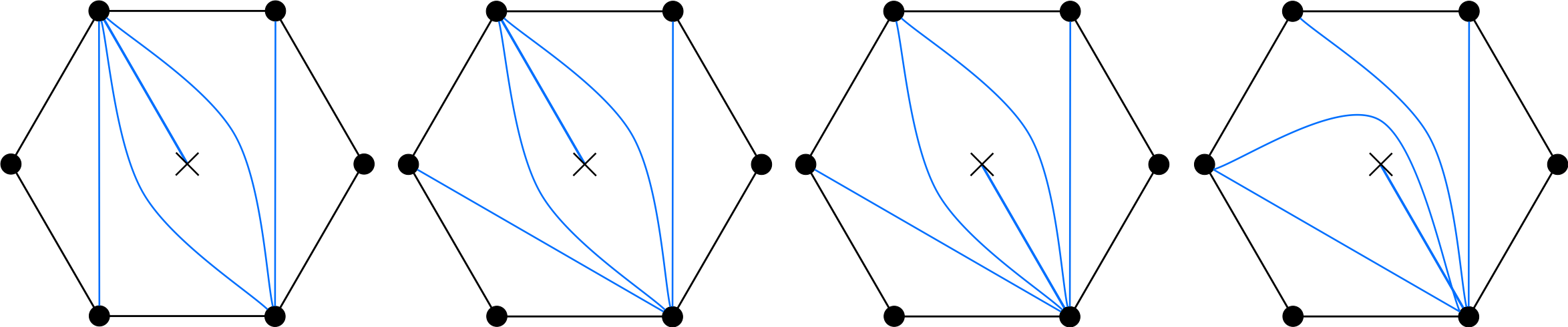
Figure 1.

Every two consecutive triangulations in the figure are clearly related by a flip.

It will be quite essential for our arguments that every triangulation can be glued from a finite number of “puzzle pieces”. For a more precise statement of what this means see [18] or [27]. Each of the puzzle pieces needed in the gluing occurs in the list depicted in Figure 2.

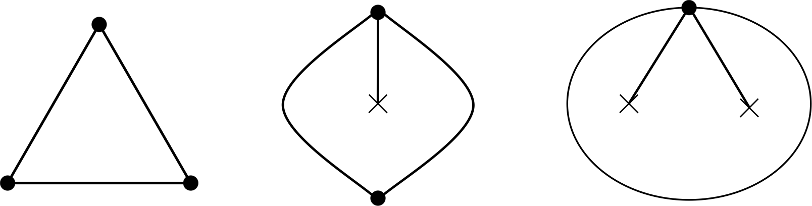
Figure 2.

In particular, the possibilities for how a triangle in a triangulation of one of the surfaces in our setting (unpunctured, or once-punctured closed) can look like are limited. More precisely, we can distinguish the following three types of triangles:

1. Ordinary triangles, i.e. triangles containing no orbifold points.

2. Once orbifolded triangles, i.e. triangles containing exactly one orbifold point.

3. Twice orbifolded triangles, i.e. triangles containing containing exactly two orbifold points.

As already mentioned in the Introduction, our input information will consist not only of a surface ${\mathbf{\Sigma}}$, but of an assignment of a weight to each orbifold point.

Definition 2.5.

A surface with marked points and weighted orbifold points ${\mathbf{\Sigma}_{\omega}}$, is a surface ${\mathbf{\Sigma}}=(\Sigma,\mathbb{M},\mathbb{O})$ together with a function $\omega:\mathbb{O}\to\{1,4\}$.

Given a function $\omega:\mathbb{O}\to\{1,4\}$ and a triangulation $\tau$ of ${\mathbf{\Sigma}}$, we denote by $\tau^{\omega=1}$ the subset of arcs in $\tau$ consisting of all pending arcs whose orbifold point $q$ has weight $\omega(q)=1$.

Remark 2.6.

1. The idea of taking a function $\omega:\mathbb{O}\rightarrow\{1,4\}$ as part of the input information comes from [18]; letting $\omega$ vary allows to associate $2^{|\mathbb{O}|}$ skew-symmetrizable matrices to any given $\tau$.

2. The number $\omega(q)\in\{1,4\}$ is never the order of $q$ as an orbifold point (as already mentioned, the order is always $2$ in our setting).

3. The reader may wonder where it is exactly that the order of the orbifold points being 2 plays a role. The role is subtly played in Felikson-Shapiro-Tumarkin’s definition of the notion of triangulation of ${\mathbf{\Sigma}}$ (Definition 2.2), as this notion is subtly tailored so that if a Fuchsian group $\Gamma\subseteq\operatorname{Iso}(\mathbb{H}^{2})$ is given with the properties that all its non-trivial finite subgroups have order 2 and some fundamental domain $D\subseteq\mathbb{H}^{2}$ of $\Gamma$ has finitely many sides and finite hyperbolic area, then any triangulation of $D$ by hyperbolic geodesics is mapped to a combinatorial triangulation of the corresponding surface with orbifold points under the projection $\mathbb{H}^{2}\rightarrow\mathbb{H}^{2}/\Gamma$, and the flip of a hyperbolic geodesic passing through a fixed point of an elliptic Möbius transformation (necessarily of order 2) is mapped to the combinatorial flip of a pending arc. See [27, the discussion that follows Definition 2.8]

For the rest of the article, ${\mathbf{\Sigma}}_{\omega}=(\Sigma,\mathbb{M},\mathbb{O},\omega)$ will be part of our a priori given input, and we will put the triangulations of ${\mathbf{\Sigma}}$ to vary only after ${\mathbf{\Sigma}}_{\omega}$ is fixed. We will denote by $\mathbf{g}$ the genus and by $b$ the number of boundary components of $\Sigma$. Moreover, we set $m=|\mathbb{M}|$, $o=|\mathbb{O}|$, and $u=|\{q\in\mathbb{O}\ |\ \omega(q)=1\}|$. Observe that by our definitions $m\geq b>0$ and $o\geq u\geq 0$.

3. The weighted quivers of a triangulation

Let ${\mathbf{\Sigma}}=(\Sigma,\mathbb{M},\mathbb{O})$ be a surface with orbifold points. In this section we will associate a weighted quiver $(Q({\tau,\omega}),\mathbf{d}({\tau,\omega}))$ to each pair $({\tau,\omega})$ consisting of a triangulation $\tau$ and a function $\omega:\mathbb{O}\rightarrow\{1,4\}$. We will also define two more quivers $Q^{\prime}({\tau,\omega})$ and $Q^{\prime\prime}({\tau,\omega})$, closely related to $Q({\tau,\omega})$, that will turn out to be useful for our constructions of chain complexes in Section 4. Our starting point to define $(Q({\tau,\omega}),\mathbf{d}({\tau,\omega}))$, $Q^{\prime}({\tau,\omega})$ and $Q^{\prime\prime}({\tau,\omega})$, will be to define a quiver $\overline{Q}(\tau)$ that does not depend on the function $\omega$.

Let us recall what a weighted quiver is.

Definition 3.1.

[32] A weighted quiver is a pair $(Q,\mathbf{d})$ consisting of a quiver $Q$ and a tuple $\mathbf{d}=(d_{i})_{i\in Q_{0}}$ of positive integers. The integer $d_{i}$ is called the weight of the vertex $i\in Q_{0}$.

Definition 3.2.

Let $\tau$ be a triangulation of ${\mathbf{\Sigma}}$. We construct a quiver $\overline{Q}(\tau)$ as follows:

1. We take for the vertex set of $\overline{Q}(\tau)$ the set of arcs of $\tau$, that is, $\overline{Q}_{0}(\tau)=\tau$.

2. The arrows of $\overline{Q}(\tau)$ are induced by the triangles of $\tau$. Namely, for each triangle $\triangle$ of $\tau$ and every pair $i,j\in\tau$ of arcs in $\triangle$ such that $j$ succeeds $i$ in $\triangle$ with respect to the orientation of $\Sigma$, we draw a single arrow from $i$ to $j$. Explicitly, for the three possible kinds of triangles depicted in Figure 2 we draw arrows according to the rule depicted in Figure 3, with the understanding that no arrow incident to a boundary segment is drawn.

   

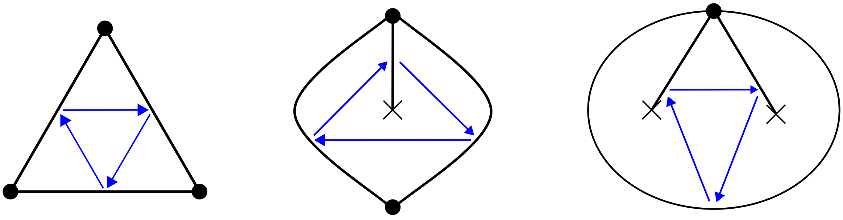
   Figure 3.

Definition 3.3.

Let ${\mathbf{\Sigma}}=(\Sigma,\mathbb{M},\mathbb{O})$ be a surface with orbifold points, $\omega:\mathbb{O}\rightarrow\{1,4\}$ a function, and $\tau$ a triangulation of ${\mathbf{\Sigma}}$. For each arc $i\in Q_{0}(\tau)$ we define an integer ${d({\tau,\omega})_{i}}$, the weight of $i$ with respect to $\omega$, by the rule

$${d({\tau,\omega})_{i}}\>=\>\begin{cases}2&\text{if $i$ is a non-pending arc,}\\ \omega(q)&\text{if $i$ is a pending arc with $q\in i\cap\mathbb{O}$.}\end{cases}$$

We set $\mathbf{d}({\tau,\omega})=({d({\tau,\omega})_{i}})_{i\in\tau}$, and define the weighted quiver of $\tau$ with respect to $\omega$ to be the weighted quiver $(Q({\tau,\omega}),\mathbf{d}({\tau,\omega}))$ on the vertex set $Q_{0}({\tau,\omega})=\tau$, where $Q({\tau,\omega})$ is the quiver obtained from $\overline{Q}(\tau)$ by adding an extra arrow $j\rightarrow i$ for each pair of pending arcs $i$ and $j$ that satisfy ${d({\tau,\omega})_{i}}={d({\tau,\omega})_{j}}$ and for which $\overline{Q}(\tau)$ has an arrow from $j$ to $i$.

Theorem 3.4.

Let ${\mathbf{\Sigma}}$, $\omega$ and $\tau$ be as in Definition 3.3. For any arc $k\in\tau$ we have $\mu_{k}(Q({\tau,\omega}),\mathbf{d}({\tau,\omega}))=(Q(f_{k}(\tau),\omega),\mathbf{d}(f_{k}(\tau),\omega))$, where $f_{k}(\tau)$ is the triangulation of ${\mathbf{\Sigma}}$ obtained from $\tau$ by flipping the arc $k$. Here, $\mu_{k}$ is the $k^{\operatorname{th}}$ mutation of weighted quivers of [32, Definition 2.5].

Remark 3.5.

1. If $\omega:\mathbb{O}\rightarrow\{1,4\}$ is the constant function taking the value $4$, then the quiver $Q({\tau,\omega})$ is the same quiver as the one defined in [27] and the weight tuple $\mathbf{d}({\tau,\omega})$ is obtained from the tuple defined in [27] by multiplying every entry of the latter by $2$.

2. According to [32, Lemma 2.3], each 2-acyclic weighted quiver $(Q,\mathbf{d})$ determines, and is determined by, a unique pair $(B,D)$ consisting of an integral skew-symmetrizable matrix $B$ and an integral diagonal matrix $D$ with positive diagonal entries such that $DB$ is skew-symmetric. On the other hand, in [18, Subsection 4.3], Felikson-Shapiro-Tumarkin associated a skew-symmetrizable matrix $B(\tau,w)$ to each pair $(\tau,w)$ consisting of a triangulation of ${\mathbf{\Sigma}}$ and a function $w:\mathbb{O}\rightarrow\{\frac{1}{2},2\}$. From such a $w$ one can obtain a function $\omega:\mathbb{O}\rightarrow\{1,4\}$ by setting $\omega(q)=\frac{2}{w(q)}$ for $q\in\mathbb{O}$ (see [27, Remark 4.7(4)]). The weighted quiver $(Q({\tau,\omega}),\mathbf{d}({\tau,\omega}))$ turns out to correspond to the pair $(B(\tau,w),\operatorname{diag}(\mathbf{d}({\tau,\omega})))$ under [32, Lemma 2.3]. So, Definition 3.3 is really due to Felikson-Shapiro-Tumarkin [18], and so is Theorem 3.4. Actually, Theorem 3.4 is one of the main motivations for the present work.

3. In [23], Fomin-Zelevinsky associate a so-called diagram to each pair $(B,D)$ as above. The quiver $\overline{Q}(\tau)$ turns out to be the diagram of $(B(\tau,w),\operatorname{diag}(\mathbf{d}({\tau,\omega})))$.

Definition 3.6.

Let ${\mathbf{\Sigma}}$, $\omega$ and $\tau$ be as in Definition 3.3. Define quivers $Q^{\prime}({\tau,\omega})$ and $Q^{\prime\prime}({\tau,\omega})$ as follows:

1. $Q^{\prime}({\tau,\omega})$ is the full subquiver of $\overline{Q}(\tau)$ spanned by the vertices $\tau\setminus\tau^{\omega=1}$. We denote by $\kappa$ the quiver morphism $Q^{\prime}({\tau,\omega})\to Q({\tau,\omega})$ obtained as the composition of the canonical inclusions $Q^{\prime}({\tau,\omega})\hookrightarrow\overline{Q}(\tau)\hookrightarrow Q({\tau,\omega})$.

2. $Q^{\prime\prime}({\tau,\omega})$ is the quiver obtained from $Q^{\prime}({\tau,\omega})$ by adding, for each arc $k\in\tau^{\omega=1}$, an arrow $\varepsilon^{\tau}_{k}$ with head and tail given by the following description:
   

   • The triangle $\triangle$ containing $k$ either contains exactly one element $i$ of the set $\tau\setminus\tau^{\omega=1}=Q^{\prime\prime}_{0}({\tau,\omega})$ (in which case $\triangle$ either contains exactly two orbifold points of weight $1$, or is a non-interior orbifolded triangle containing exactly one pending arc, being $k$ this one; see 2), or $\triangle$ contains exactly two elements $i,j$ from $\tau\setminus\tau^{\omega=1}=Q^{\prime\prime}_{0}({\tau,\omega})$ and induces an arrow $\alpha$ of $Q({\tau,\omega})$ that goes from one of these arcs to the other, say from $i=t(\alpha)$ to $j=h(\alpha)$. In the former case, we set $h(\varepsilon^{\tau}_{k})=t(\varepsilon^{\tau}_{k})=i$, and, in the latter case, $h(\varepsilon^{\tau}_{k})=i$ and $t(\varepsilon^{\tau}_{k})=j$.

Remark 3.7.

Note that the quivers $Q({\tau,\omega})$, $Q^{\prime}({\tau,\omega})$, and $Q^{\prime\prime}({\tau,\omega})$ are connected.

Example 3.8.

In Figure 4 we can see two triangulations $\tau$ and $\sigma$ of the pentagon with two orbifold points.

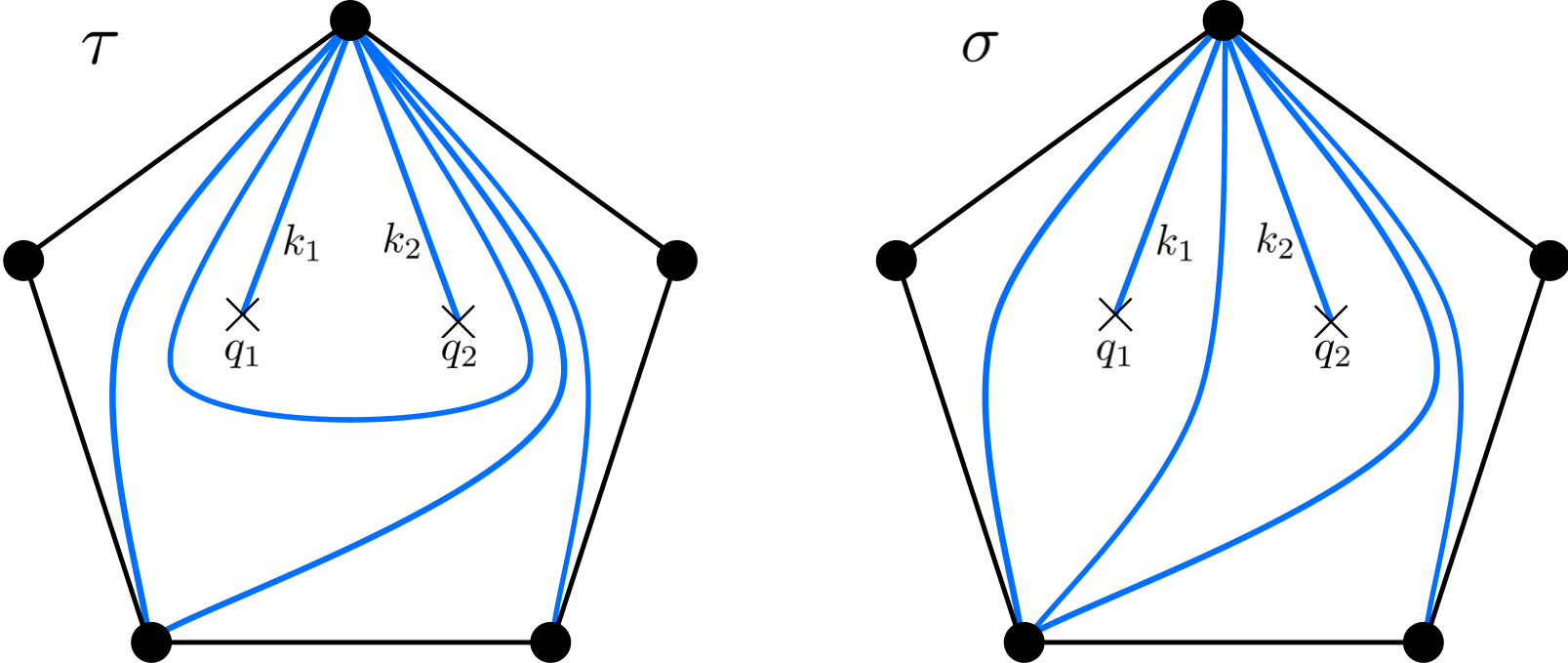
Figure 4.

The quivers $\overline{Q}(\tau)$ and $\overline{Q}(\sigma)$ are:

The quivers $Q({\tau,\omega})$, $Q^{\prime}({\tau,\omega})$, $Q^{\prime\prime}({\tau,\omega})$, $Q(\sigma,\omega)$, $Q^{\prime}(\sigma,\omega)$ and $Q^{\prime\prime}(\sigma,\omega)$ can be seen in Figures 5 and 6 for all possible functions $\omega:\mathbb{O}\rightarrow\{1,4\}$.

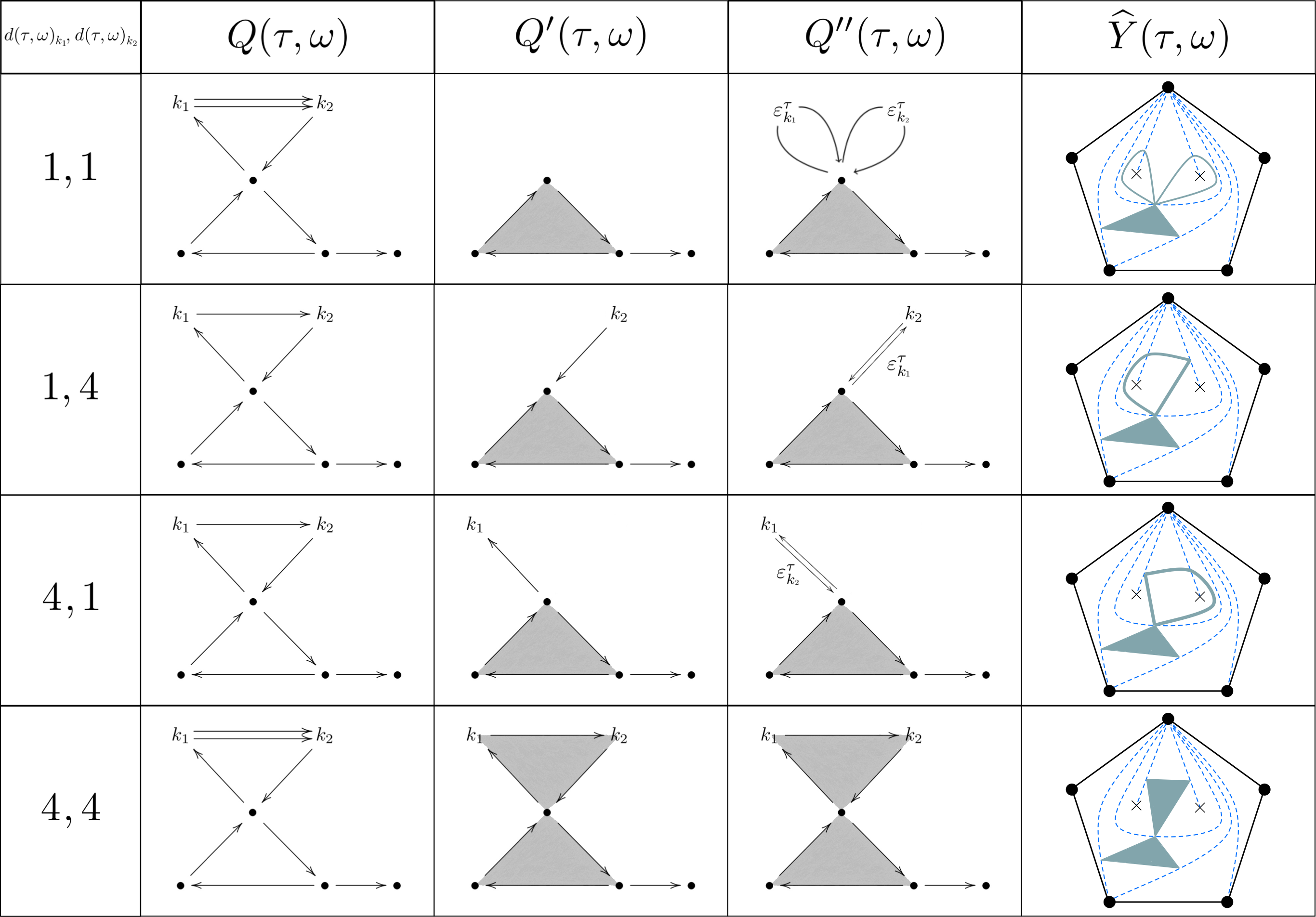
Figure 5.

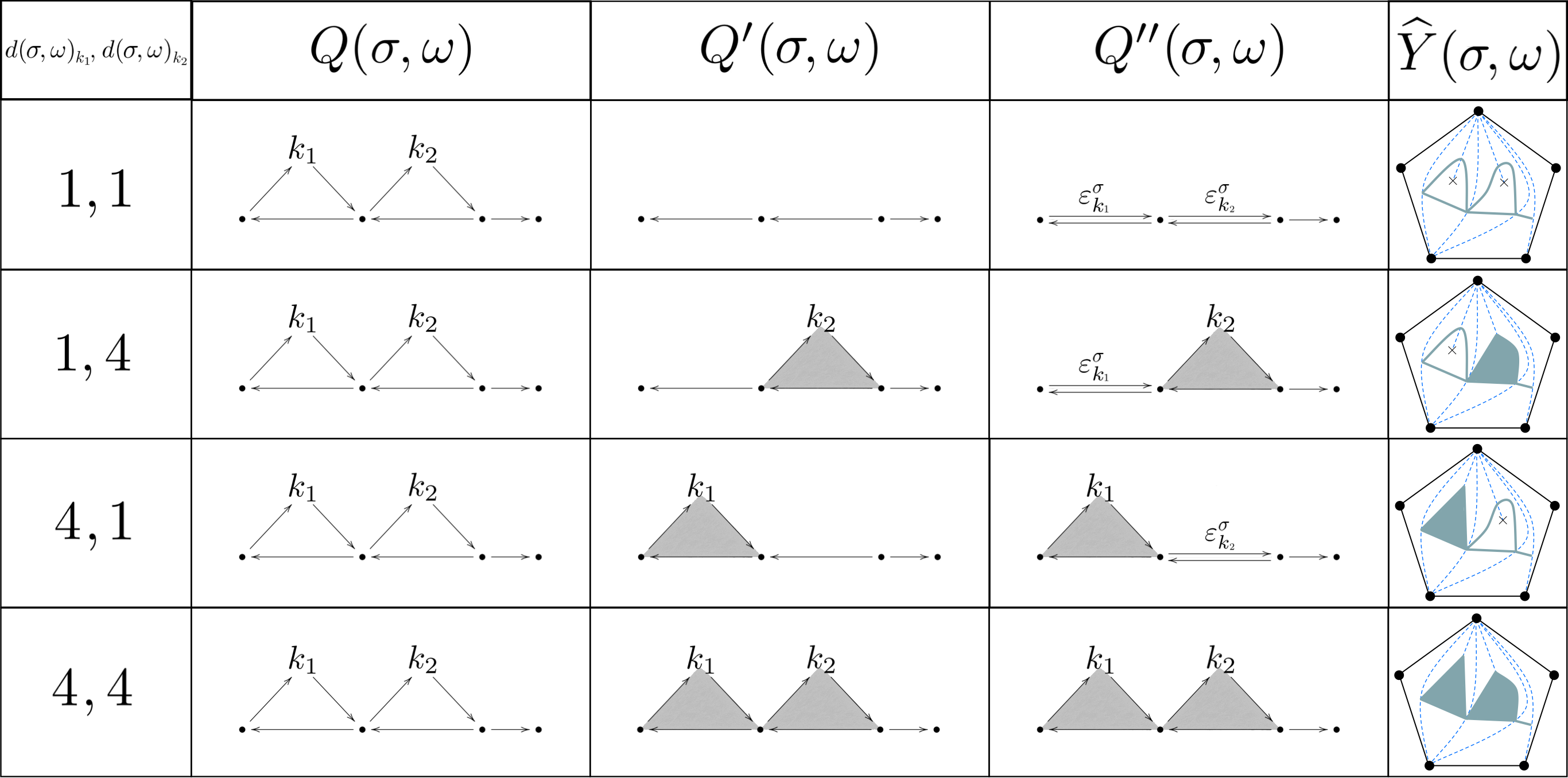
Figure 6.

Note that no triangle of $\sigma$ contains more than one orbifold point, hence $Q(\sigma,\omega)=\overline{Q}(\sigma)$ for every function $\omega:\mathbb{O}\rightarrow\{1,4\}$.

4. Chain complexes associated with a triangulation

We begin this section with an example intended to motivate the constructions that are to come.

Example 4.1.

Let ${\mathbf{\Sigma}}=(\Sigma,\mathbb{M},\mathbb{O})$ be the unpunctured pentagon with two orbifold points. Consider the triangulation $\sigma$ of ${\mathbf{\Sigma}}$ depicted in Figure 4 and the function $\omega:\mathbb{O}\rightarrow\{1,4\}$ given by $\omega(q_{1})=4$ and $\omega(q_{2})=1$. Let $F$ be a field containing a primitive $4^{\operatorname{th}}$ root of unity, $E/F$ a degree-$4$ cyclic Galois extension, and $L$ the unique subfield of $E$ that has degree $2$ over $F$. In order to define a species realization of the weigted quiver $(Q(\sigma,\omega),\mathbf{d}(\sigma,\omega))$ using this data, we still need a modulating function $g:Q_{1}(\sigma,\omega)\rightarrow\bigcup_{i,j\in\sigma}\operatorname{Gal}(F_{i,j}/F)=\operatorname{Gal}(E/F)\cup\operatorname{Gal}(L/F)\cup\operatorname{Gal}(F/F)$ (see [27, Section 3] for definitions and notation). An easy count shows that there are $2^{5}$ such functions. However, [27, Example 3.12] shows that for some of these $2^{5}$ modulating functions the corresponding species fails to admit a non-degenerate potential.

Let us be more precise about the last statement. As pointed out in Example 3.8, the quiver of $(\sigma,\omega)$ is

Let $g:Q_{1}(\sigma,\omega)\rightarrow\bigcup_{i,j\in\sigma}\operatorname{Gal}(F_{i,j}/F)$ be any modulating function for $Q(\sigma,\omega)$, and let $A_{g}$ be the corresponding species (cf. [27, Definitions 3.2 and 3.3], where $g$ does not appear as subindex). Then $g_{\alpha},g_{\beta},g_{\gamma}\in\operatorname{Gal}(L/F)\cong\mathbb{Z}/2\mathbb{Z}$. Applying [27, Example 3.12] to the species $\widetilde{\mu}_{k_{1}}(A_{g})$ shows that if $g_{\alpha}g_{\beta}g_{\gamma}\neq 11_{L}$, then for any potential $S\in R\langle\langle A_{g}\rangle\rangle$ the SP $(A_{g},S)$ is degenerate.

So, if we want a species realization of $(Q(\sigma,\omega),\mathbf{d}(\sigma,\omega))$ that has the chance to admit a non-degenerate potential, we must restrict our attention to those modulating functions $g$ which satisfy $g_{\alpha}g_{\beta}g_{\gamma}=11_{L}\in\operatorname{Gal}(L/F)$. A moment of thought tells us that this is a cocycle condition inside some cochain complex with coefficientes in $\operatorname{Gal}(L/F)\cong\mathbb{Z}/2\mathbb{Z}$.

One is thus tempted to work with (the cochain complex which is $\mathbb{F}_{2}$-dual to) the chain complex with coefficients in $\mathbb{F}_{2}:=\mathbb{Z}/2\mathbb{Z}$ defined by taking $Q_{0}(\sigma,\omega)$ and $Q_{1}(\sigma,\omega)$ as $\mathbb{F}_{2}$-bases of the $0^{\operatorname{th}}$ and $1^{\operatorname{st}}$ chain groups, and the set consisting of the two “obvious” 3-cycles on $Q(\sigma,\omega)$ as a $\mathbb{F}_{2}$-basis of the $2^{\operatorname{nd}}$ chain group, with the differentials defined in an obvious way (so that the image of each of the two “obvious” 3-cycles under the $2^{\operatorname{nd}}$ differential is the sum of the three arrows that appear in it). This is, however, not quite the chain complex whose dual cochain complex we will need to consider. Indeed, since $\omega(q_{2})=1$ in the current example, every modulating function $g:Q_{1}(\sigma,\omega)\rightarrow\bigcup_{i,j\in\sigma}\operatorname{Gal}(F_{i,j}/F)$ satisfies $g_{\eta}|_{F}g_{\nu}g_{\rho}=11_{F}\in\operatorname{Gal}(F/F)$, so there is no need to impose any no cocycle condition on the 3-cycle passing through $k_{2}$.

Let us go back to general considerations; fix again a triangulation $\tau$ of ${\mathbf{\Sigma}}$ and a function $\omega:\mathbb{O}\rightarrow\{1,4\}$. We define a family of sets $X_{\bullet}({\tau,\omega})=(X_{n}({\tau,\omega}))_{n\in\mathbb{N}}$ by setting $X_{n}({\tau,\omega})=\varnothing$ for $n\not\in\{0,1,2\}$ and

(4.1) $$\begin{array}[]{lcl}X_{0}({\tau,\omega})&=&Q^{\prime}_{0}({\tau,\omega}),\\[5.0pt] X_{1}({\tau,\omega})&=&Q^{\prime}_{1}({\tau,\omega}),\\[5.0pt] X_{2}({\tau,\omega})&=&\{\triangle\ |\ \text{$\triangle$ is an interior triangle of $\tau$ all of whose arcs belong to $X_{0}({\tau,\omega})$}\}.\end{array}$$

We define $\widehat{X}_{\bullet}({\tau,\omega})=(\widehat{X}_{n}({\tau,\omega}))_{n\in\mathbb{N}}$ as the family of sets given by

(4.2) $$\widehat{X}_{n}({\tau,\omega})=\begin{cases}Q^{\prime\prime}_{1}({\tau,\omega})=X_{1}({\tau,\omega})\cup\{{{\varepsilon^{\tau}_{k}}}\ |\ \text{$k\in\tau^{\omega=1}$}\}&\text{if $n=1$,}\\ X_{n}({\tau,\omega})&\text{if $n\neq 1$.}\end{cases}$$

Similarly to [4, Subsection 2.2], we can define a chain complex ${C_{\bullet}({\tau,\omega})}$ associated with $X_{\bullet}({\tau,\omega})$ that embeds canonically into a chain complex ${\widehat{C}_{\bullet}({\tau,\omega})}$ associated with $\widehat{X}_{\bullet}({\tau,\omega})$ as follows:

(4.3)

where $\mathbb{F}_{2}X$ stands for the vector space with basis $X$ over $\mathbb{F}_{2}=\mathbb{Z}/2\mathbb{Z}$. The non-zero differentials are given on basis elements as follows:

$$\begin{array}[]{lcll}\partial_{2}(\triangle)&=&{{\alpha}}+{{\beta}}+{{\gamma}}&\hskip 5.0pt\text{if \smash{$\triangle\in\widehat{X}_{2}({\tau,\omega})$} induces $\alpha,\beta,\gamma\in Q^{\prime}_{1}({\tau,\omega})$,}\\[5.0pt] \partial_{1}({{\alpha}})&=&h(\alpha)-t(\alpha)&\hskip 5.0pt\text{for \smash{${{\alpha}}\in\widehat{X}_{1}({\tau,\omega})$}.}\end{array}$$

Remark 4.2.

We will use the 1-cocycles of the cochain complex which is $\mathbb{F}_{2}$-dual to ${C_{\bullet}({\tau,\omega})}$ to choose modulating functions on $(Q(\tau,\omega),\mathbf{d}(\tau,\omega))$. It is to define the flips on these 1-cocycles that we will use the auxiliary chain complex ${\widehat{C}_{\bullet}({\tau,\omega})}$, for the flip rule on 1-cocycles will not always be the obvious $\mathbb{F}_{2}$-linear function one may come up with.

Example 4.3.

Let ${\mathbf{\Sigma}}$ be the unpunctured pentagon with two orbifold points, and let $\tau$ and $\sigma$ be the triangulations of ${\mathbf{\Sigma}}$ depicted in Figure 4. In the third column of Figure 5 (resp. Figure 6) we can visualize the sets $X_{0}({\tau,\omega})$, $X_{1}({\tau,\omega})$ and $X_{2}({\tau,\omega})$ (resp. $X_{0}(\sigma,\omega)$, $X_{1}(\sigma,\omega)$ and $X_{2}(\sigma,\omega)$) for all possible functions $\omega:\mathbb{O}\rightarrow\{1,4\}$, while in the fourth column we can visualize the sets $\widehat{X}_{0}({\tau,\omega})$, $\widehat{X}_{1}({\tau,\omega})$ and $\widehat{X}_{2}({\tau,\omega})$ (resp. $\widehat{X}_{0}(\sigma,\omega)$, $\widehat{X}_{1}(\sigma,\omega)$ and $\widehat{X}_{2}(\sigma,\omega)$). The shaded triangular regions correspond to the elements of the respective set $\widehat{X}_{2}({\tau,\omega})$ (or $\widehat{X}_{2}(\sigma,\omega)$). Note that for those functions $\omega$ that take the value $1$ at least once, the dimension over $\mathbb{F}_{2}$ of the first homology group of the corresponding chain complex ${\widehat{C}_{\bullet}({\tau,\omega})}$ (resp. $\widehat{C}_{\bullet}(\sigma,\omega)$) is strictly greater than the dimension over $\mathbb{F}_{2}$ of the first homology group of the chain complex ${C_{\bullet}({\tau,\omega})}$ (resp. $C_{\bullet}(\sigma,\omega)$).

5. Colored triangulations and their flips

Let ${\mathbf{\Sigma}}=(\Sigma,\mathbb{M},\mathbb{O})$ be a surface with (arbitrarily many) orbifold points which is either unpunctured with non-empty boundary, or once-punctured closed. The main combinatorial input for our construction of species and potentials will be colored triangulations.

Definition 5.1.

A colored triangulation of ${\mathbf{\Sigma}_{\omega}}$ is a pair $(\tau,\xi)$ consisting of a triangulation $\tau$ of ${\mathbf{\Sigma}}$ and a $1$-cocycle $\xi$ of the cochain complex ${C^{\bullet}({\tau,\omega})}=\operatorname{Hom}_{\mathbb{F}_{2}}({C_{\bullet}({\tau,\omega})},\mathbb{F}_{2})$.

For each triangulation $\tau$ of ${\mathbf{\Sigma}}$ and each function $\omega:\mathbb{O}\rightarrow\{1,4\}$ we will denote by ${Z^{1}({\tau,\omega})}$ the set of $1$-cocycles of ${C^{\bullet}({\tau,\omega})}$. Thus, ${Z^{1}({\tau,\omega})}$ is an $\mathbb{F}_{2}$-vector subspace of $C^{1}(\tau,\omega)$.

Remark 5.2.

By its very definition, $C_{1}(\tau,\omega)$ is the $\mathbb{F}_{2}$-vector space with basis $Q^{\prime}_{1}({\tau,\omega})$. Let $\{{{\alpha}}^{\vee}\ |\ \alpha\in Q^{\prime}_{1}({\tau,\omega})\}$ be the $\mathbb{F}_{2}$-vector space basis of $C^{1}(\tau,\omega)=\operatorname{Hom}_{\mathbb{F}_{2}}(C_{1}(\tau,\omega),\mathbb{F}_{2})$ which is dual to $Q^{\prime}_{1}({\tau,\omega})$. Then, choosing a cocycle $\xi=\sum_{{{\alpha}}}\xi({{\alpha}}){{\alpha}}^{\vee}\in{Z^{1}({\tau,\omega})}$ amounts to fixing, for each arrow ${{\alpha}}\in Q^{\prime}_{1}({\tau,\omega})$, an element $\xi({{\alpha}})\in\{0,1\}=\mathbb{F}_{2}$ in such a way that whenever ${{\alpha}},{{\beta}},{{\gamma}}$ are arrows of $Q^{\prime}({\tau,\omega})$ induced by an interior triangle $\triangle$ one has

$$\xi({{\alpha}})+\xi({{\beta}})+\xi({{\gamma}})=0\>\in\>\mathbb{F}_{2}\,.$$

As we will see in Section 11, without this condition the corresponding species would fail to admit a non-degenerate potential, a fact that was hinted already in Example 4.1.

In this section we want to explain how to obtain one colored triangulation from another by flipping an arc. For this purpose let us fix two triangulations $\tau$ and $\sigma$ of ${\mathbf{\Sigma}}$ that are related by the flip of an arc $k\in\sigma$ in the sense of [18]. Our goal is to define a “natural” bijection ${Z^{1}({\tau,\omega})}\to{Z^{1}({\sigma,\omega})}$.

Consider the morphism $\rho_{\tau}:{\widehat{C}_{\bullet}({\tau,\omega})}\to{C_{\bullet}({\tau,\omega})}$ defined as $(\rho_{\tau})_{n}=\mathrm{id}_{\widehat{C}_{n}({\tau,\omega})}$ for $n\neq 1$, and by the rule

$$(\rho_{\tau})_{1}({{\alpha}})\>=\>\begin{cases}\phantom{-}{{\alpha}}&\text{if ${{\alpha}}\in X_{1}({\tau,\omega})$,}\\ -{{\beta}}&\text{if ${{\alpha}}={{\varepsilon^{\tau}_{k}}}$ and there exists ${{\beta}}\in Q_{1}^{\prime}({\tau,\omega})$ induced by a triangle containing~{}$k$,}\\ \phantom{-\,\,}0&\text{otherwise.,}\end{cases}$$

for ${{\alpha}}\in\widehat{X}_{1}({\tau,\omega})$. It is easy to check that $\rho_{\tau}$ is indeed a morphism of chain complexes. Let us denote by $\rho^{\tau}$ the dual morphism ${C^{\bullet}({\tau,\omega})}\to{\widehat{C}^{\bullet}({\tau,\omega})}$ induced by $\rho_{\tau}$, where ${\widehat{C}^{\bullet}({\tau,\omega})}=\operatorname{Hom}_{\mathbb{F}_{2}}({\widehat{C}_{\bullet}({\tau,\omega})},\mathbb{F}_{2})$.

Remark 5.3.

Clearly, $\rho_{\tau}$ is surjective and $\rho^{\tau}$ injective. Moreover, in cohomology $\rho^{\tau}$ is a section of the morphism ${H^{\bullet}(\widehat{C}^{\bullet}({\tau,\omega}))}\twoheadrightarrow{H^{\bullet}(C^{\bullet}({\tau,\omega}))}$ induced by the canonical inclusion $X_{\bullet}({\tau,\omega})\hookrightarrow\widehat{X}_{\bullet}({\tau,\omega})$.

Recall from (4.1), (4.2) and (4.3) that $\widehat{X}_{1}({\tau,\omega})=Q^{\prime}_{1}({\tau,\omega})\cup\{{{\varepsilon^{\tau}_{k}}}\ |\ k\in\tau^{\omega=1}\}$ is an $\mathbb{F}_{2}$-basis of $\widehat{C}_{1}(\tau,\omega)$; let $\{\alpha^{\vee}\ |\ \alpha\in\widehat{X}_{1}({\tau,\omega})\}$ be the corresponding dual $\mathbb{F}_{2}$-basis of $\widehat{C}^{1}(\tau,\omega)=\operatorname{Hom}_{\mathbb{F}_{2}}(\widehat{C}_{1}(\tau,\omega),\mathbb{F}_{2})$. Denote by ${\widehat{Z}^{1}({\tau,\omega})}$ the set of $1$-cocycles of ${\widehat{C}^{\bullet}({\tau,\omega})}$. We associate with each cocycle $\xi\in{Z^{1}({\tau,\omega})}$ the cocycle

$$\widehat{\xi}\>=\>\rho^{\tau}(\xi)+\varepsilon^{\tau}\>\in\>{\widehat{Z}^{1}({\tau,\omega})}\,,$$

where $\varepsilon^{\tau}$ is the cocycle $\sum_{k\in\tau^{\omega=1}}({{\varepsilon^{\tau}_{k}}})^{\vee}$.

Example 5.4.

Consider once more the triangulation $\tau$ depicted in Figure 4. In Figure 7 we illustrate the function $\xi\mapsto\widehat{\xi}$ for all possible functions $\omega:\mathbb{O}\rightarrow\{1,4\}$.

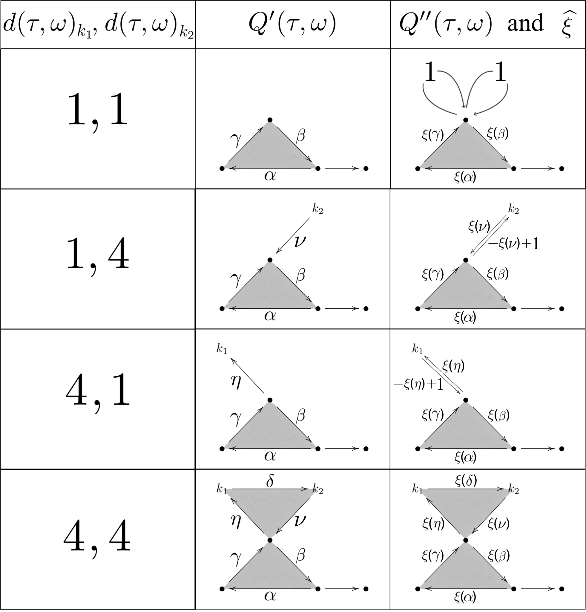
Figure 7.

More precisely, in the left-most column we have written the possible values of $\omega$, the middle column depicts the corresponding quiver $Q^{\prime}(\tau,\omega)$, with its arrows labeled with their names, and the right-most column depicts the quiver $Q^{\prime\prime}(\tau,\omega)$, with its arrows labeled not with their names, but with the values that $\widehat{\xi}$ takes at them for any given $\xi\in Z^{1}(\tau,\omega)$.

The following easy observation will become important in Section 9.

Lemma 5.5.

Let $(\tau,\xi)$ and $(\tau,\xi^{\prime})$ be two colored triangulations of ${\mathbf{\Sigma}_{\omega}}$. Then $[\xi]=[\xi^{\prime}]$ in ${H^{1}(C^{\bullet}({\tau,\omega}))}$ if and only if $\big{[}\widehat{\xi}\,\big{]}=\big{[}\widehat{\xi}^{\prime}\big{]}$ in ${H^{1}(\widehat{C}^{\bullet}({\tau,\omega}))}$.

Proof.

Because of the injectivity of $\rho^{\tau}$ in cohomology, $\big{[}\widehat{\xi}-\widehat{\xi^{\prime}}\big{]}=\rho^{\tau}([\xi-\xi^{\prime}])=0$ if and only if $[\xi-\xi^{\prime}]=0$. ∎

To compare the complexes ${\widehat{C}_{\bullet}({\sigma,\omega})}$ and ${\widehat{C}_{\bullet}({\tau,\omega})}$, we define a morphism $\varphi_{\tau,\sigma}:{\widehat{C}_{\bullet}({\sigma,\omega})}\to{\widehat{C}_{\bullet}({\tau,\omega})}$ as follows. For notational simplicity we will make the identification $k=k^{\prime}$ for the unique arc $k^{\prime}\in\tau\setminus\sigma$, so that we have $C_{0}({\sigma,\omega})=C_{0}({\tau,\omega})$. Thus, we can set $(\varphi_{\tau,\sigma})_{0}=\mathrm{id}_{C_{0}({\sigma,\omega})}$.

Next, define $(\varphi_{\tau,\sigma})_{2}:{\widehat{C}_{\bullet}({\sigma,\omega})}\to{\widehat{C}_{\bullet}({\tau,\omega})}$ following the rule

$$(\varphi_{\tau,\sigma})_{2}(\triangle)=\begin{cases}\triangle&\text{if $\triangle$ does not contain $k$,}\\ 0&\text{if $\triangle$ contains $k$,}\end{cases}$$

for $\triangle\in\widehat{X}_{2}({\sigma,\omega})$.

Finally, we shall define $\varphi_{\tau,\sigma}({{\alpha}})=(\varphi_{\tau,\sigma})_{1}({{\alpha}})$ for every ${{\alpha}}\in\widehat{X}_{1}({\sigma,\omega})$.

For $\rho\in\{\sigma,\tau\}$ let $Q^{k}({\rho,\omega})$ be the subquiver of $Q^{\prime\prime}({\rho,\omega})$ spanned by all arrows that are induced by the triangles containing $k$, including arrows of the form $\varepsilon^{\tau}_{i}$ for $i$ contained in any triangle containing $k$. Notice that $Q^{k}({\rho,\omega})$ may fail to be a full subquiver of $Q^{\prime\prime}({\rho,\omega})$.

Let us call a triangle of $\rho\in\{\sigma,\tau\}$ exceptional if it is an interior triangle and contains exactly one arc $\ell$ with $d(\rho,\omega)_{\ell}=1$. Note that any exceptional triangle of $\rho$ is necessarily orbifolded (although it may contain two orbifold points), and induces a unique arrow ${{\delta^{\rho}_{\ell}}}\in Q_{1}({\rho,\omega})$ not incident to $\ell$.

For every ${{\alpha}}\in Q^{\prime\prime}_{1}({\sigma,\omega})\setminus Q^{k}_{1}({\sigma,\omega})=Q^{\prime\prime}_{1}({\tau,\omega})\setminus Q^{k}_{1}({\tau,\omega})$ we set $\varphi_{\tau,\sigma}({{\alpha}})={{\alpha}}$.

Let ${{\alpha}}\in Q^{k}_{1}({\sigma,\omega})$. If $k$ is a pending arc of weight $1$ in an exceptional triangle of $\sigma$, set

$$\varphi_{\tau,\sigma}({{\alpha}})\>=\>\begin{cases}{{\varepsilon^{\tau}_{k}}}&\text{if ${{\alpha}}={{\delta^{\sigma}_{k}}}$,}\\ {{\delta^{\tau}_{k}}}&\text{if ${{\alpha}}={{\varepsilon^{\sigma}_{k}}}$.}\end{cases}$$

If $k$ is a pending arc of weight $4$ in an exceptional triangle of $\sigma$ whose other pending arc is $\ell\in\tau^{\omega=1}$, set

$$\varphi_{\tau,\sigma}({{\alpha}})\>=\>\begin{cases}-{{\delta^{\tau}_{\ell}}}&\text{if ${{\alpha}}={{\delta^{\sigma}_{\ell}}}$,}\\ -{{\varepsilon^{\tau}_{\ell}}}&\text{if ${{\alpha}}={{\varepsilon^{\sigma}_{\ell}}}$,}\end{cases}$$

and, finally, if $k$ is not a pending arc in an exceptional triangle of $\sigma$, we set

(5.1) $$\varphi_{\tau,\sigma}({{\alpha}})\>=\>\begin{cases}{{\mu^{\tau}_{\ell}}}+{{\varepsilon^{\tau}_{\ell}}}+{{\nu^{\tau}_{\ell}}}&\text{if ${{\alpha}}={{\varepsilon^{\sigma}_{\ell}}}$,}\\ \>\>\>\>\>\>\>-{{\alpha^{*}}}&\text{if ${{\alpha}}\in X_{1}({\sigma,\omega})$ with $h({{\alpha}})=k$ or $t({{\alpha}})=k$,}\\ \>\>\>\>{{\beta^{*}}}+{{\gamma^{*}}}&\text{if ${{\alpha}}\in X_{1}({\sigma,\omega})$ with $h({{\alpha}})\neq k$ and $t({{\alpha}})\neq k$, where ${{\beta}}$, ${{\gamma}}$ with $h(\gamma)=k$}\\ &\raisebox{2.0pt}{\text{and $t(\beta)=k$ are induced by the same $\triangle\in X_{2}({\sigma,\omega})$ as ${{\alpha}}$.}}\vspace{-2pt}\end{cases}$$

Here, if ${{\alpha}}={{\varepsilon^{\sigma}_{\ell}}}$, then the elements ${{\mu^{\tau}_{\ell}}}$ and ${{\nu^{\tau}_{\ell}}}$ of ${\widehat{C}_{1}({\tau,\omega})}$ are given as follows:

(5.2) $$\begin{array}[]{lll}{{\mu^{\tau}_{\ell}}}&=&\begin{cases}{{\mu}}&\text{if $t(\varepsilon^{\tau}_{\ell})\neq t(\varepsilon^{\sigma}_{\ell})$ and ${{\mu}}\in Q_{1}({\tau,\omega})$ with $t({{\mu}})=t(\varepsilon^{\sigma}_{\ell})$ and $h({{\mu}})=t(\varepsilon^{\tau}_{\ell})$,}\\ 0&\text{otherwise,}\end{cases}\\[16.99998pt] {{\nu^{\tau}_{\ell}}}&=&\begin{cases}{{\nu}}&\text{if $h(\varepsilon^{\tau}_{\ell})\neq h(\varepsilon^{\sigma}_{\ell})$ and ${{\nu}}\in Q_{1}({\tau,\omega})$ with $t({{\nu}})=h(\varepsilon^{\tau}_{\ell})$ and $h({{\nu}})=h(\varepsilon^{\sigma}_{\ell})$,}\\ 0&\text{otherwise.}\end{cases}\end{array}$$

The following lemma will be essential later on.

Lemma 5.6.

Let $\sigma$ be a triangulation of ${\mathbf{\Sigma}}$ related to $\tau$ by the flip of an arc $k$. The $\mathbb{F}_{2}$-linear maps we have just defined constitute a homomorphism of chain complexes $\varphi_{\tau,\sigma}:\widehat{C}_{\bullet}(\sigma,\omega)\rightarrow\widehat{C}_{\bullet}(\tau,\omega)$. This chain complex homomorphism is a homotopy equivalence, hence the $\mathbb{F}_{2}$-linear maps $\varphi_{\tau,\sigma}^{*}=(\varphi_{\tau,\sigma})_{n}^{*}:\operatorname{Hom}_{\mathbb{F}_{2}}(\widehat{C}_{n}(\tau,\omega),\mathbb{F}_{2})\rightarrow\operatorname{Hom}_{\mathbb{F}_{2}}(\widehat{C}_{n}(\sigma,\omega),\mathbb{F}_{2})$ given by $\varphi_{\tau,\sigma}^{*}(f)=f\circ\varphi_{\tau,\sigma}$ induce an isomorphism in cohomology

$$H^{\bullet}(\widehat{C}^{\bullet}(\tau,\omega))\xrightarrow{\hskip 15.0pt}H^{\bullet}(\widehat{C}^{\bullet}(\sigma,\omega)),$$

whose inverse is induced by $\varphi_{\sigma,\tau}^{*}$. Actually, $\varphi_{\tau,\sigma}$ and $\varphi_{\sigma,\tau}$ already induce a pair of inverse isomorphisms

$$\lx@xy@svg{\hbox{\raise 0.0pt\hbox{\kern 18.30914pt\hbox{\ignorespaces\ignorespaces\ignorespaces\hbox{\vtop{\kern 0.0pt\offinterlineskip\halign{\entry@#!@&&\entry@@#!@\cr&&\crcr}}}\ignorespaces{\hbox{\kern-18.30914pt\raise 0.0pt\hbox{\hbox{\kern 0.0pt\raise 0.0pt\hbox{\hbox{\kern 3.0pt\raise 0.0pt\hbox{$\textstyle{{\widehat{Z}^{1}({\tau,\omega})}\ignorespaces\ignorespaces\ignorespaces\ignorespaces}$}}}}}}}\ignorespaces\ignorespaces\ignorespaces\ignorespaces{}{\hbox{\lx@xy@droprule}}\ignorespaces\ignorespaces\ignorespaces{\hbox{\kern 37.89365pt\raise 7.79167pt\hbox{{}\hbox{\kern 0.0pt\raise 0.0pt\hbox{\hbox{\kern 3.0pt\hbox{\hbox{\kern 0.0pt\raise-1.15279pt\hbox{$\scriptstyle{\varphi_{\tau,\sigma}^{*}}$}}}\kern 3.0pt}}}}}}\ignorespaces{\hbox{\kern 72.30914pt\raise 2.0pt\hbox{\hbox{\kern 0.0pt\raise 0.0pt\hbox{\lx@xy@tip{1}\lx@xy@tip{-1}}}}}}{\hbox{\lx@xy@droprule}}{\hbox{\lx@xy@droprule}}{\hbox{\kern 42.30914pt\raise 0.0pt\hbox{\hbox{\kern 0.0pt\raise 0.0pt\hbox{\hbox{\kern 3.0pt\raise 0.0pt\hbox{$\textstyle{}$}}}}}}}{\hbox{\kern 72.30914pt\raise 0.0pt\hbox{\hbox{\kern 0.0pt\raise 0.0pt\hbox{\hbox{\kern 3.0pt\raise 0.0pt\hbox{$\textstyle{{\widehat{Z}^{1}({\sigma,\omega})}\ignorespaces\ignorespaces\ignorespaces\ignorespaces}$}}}}}}}\ignorespaces\ignorespaces\ignorespaces\ignorespaces{}{\hbox{\lx@xy@droprule}}\ignorespaces\ignorespaces\ignorespaces{\hbox{\kern 39.35521pt\raise-7.79166pt\hbox{{}\hbox{\kern 0.0pt\raise 0.0pt\hbox{\hbox{\kern 3.0pt\hbox{\hbox{\kern 0.0pt\raise-1.15279pt\hbox{$\scriptstyle{\varphi^{*}_{\sigma,\tau}}$}}}\kern 3.0pt}}}}}}\ignorespaces{\hbox{\kern 18.30916pt\raise-2.0pt\hbox{\hbox{\kern 0.0pt\raise 0.0pt\hbox{\lx@xy@tip{1}\lx@xy@tip{-1}}}}}}{\hbox{\lx@xy@droprule}}{\hbox{\lx@xy@droprule}}\ignorespaces}}}}\ignorespaces. \textstyle{{\widehat{Z}^{1}({\tau,\omega})}\ignorespaces\ignorespaces\ignorespaces\ignorespaces} \scriptstyle{\varphi_{\tau,\sigma}^{*}} \textstyle{{\widehat{Z}^{1}({\sigma,\omega})}\ignorespaces\ignorespaces\ignorespaces\ignorespaces} \scriptstyle{\varphi^{*}_{\sigma,\tau}} \textstyle{{\widehat{Z}^{1}({\tau,\omega})}\ignorespaces\ignorespaces\ignorespaces\ignorespaces} \scriptstyle{\varphi_{\tau,\sigma}^{*}} \textstyle{{\widehat{Z}^{1}({\sigma,\omega})}\ignorespaces\ignorespaces\ignorespaces\ignorespaces} \scriptstyle{\varphi^{*}_{\sigma,\tau}}$$

Before turning to the proof of Lemma 5.6, let us shortly illustrate and motivate the definition of $\varphi_{\tau,\sigma}$. For simplicity, we assume for this illustration that the triangles of $\sigma$ with side $k$ are interior.

As will be pointed out in the proof of Theorem 7.1, there are in principle (up to interchanging $\sigma$ and $\tau$) $24$ possibilities for $(Q^{k}({\sigma,\omega}),Q^{k}({\tau,\omega}))$ corresponding to the configurations $1$, $2$, $3$, $4$, $5$, $6$, $11$, $13$, $14$, $18$, $19$, $20$, $21$, $24$, $25\>\widehat{=}\>26$, $27$, $32$, $34$, $36$, $37$, $38$, $39$, $44$, $45$ depicted in Figure 23. These configurations can be grouped together as done in Figure 8, leaving us with $9$ cases. The action of $\varphi_{\tau,\sigma}$ on $Q^{k}({\sigma,\omega})$ and of $\varphi_{\sigma,\tau}$ on $Q^{k}({\tau,\omega})$ has been unraveled in the last two columns of the table.

Remark 5.7.

To get a conceptual idea why $\varphi_{\tau,\sigma}$ “should” be defined as we just did it and why Lemma 5.6 is true, you might want to take a look at Proposition 8.9 and the discussion in Section 8 preceding it.

Figure 8.

width 1pt        Case	Configs.	$Q^{k}({\sigma,\omega})$	$Q^{k}({\tau,\omega})$	$\varphi_{\tau,\sigma}$	$\varphi_{\sigma,\tau}$   width 1pt
width 1pt        I	1, 4			$\begin{array}[]{lcl}{{\delta^{\sigma}}}&\mapsto&\varepsilon^{\tau}\\ \varepsilon^{\sigma}&\mapsto&{{\delta^{\tau}}}\end{array}$	$\begin{array}[]{lcl}{{\delta^{\tau}}}&\mapsto&\varepsilon^{\sigma}\\ \varepsilon^{\tau}&\mapsto&{{\delta^{\sigma}}}\end{array}$   width 1pt
width 1pt      II	3			$\begin{array}[]{lcl}\varepsilon^{\sigma}_{i}&\mapsto&\varepsilon^{\tau}_{i}\end{array}$	$\begin{array}[]{lcl}\varepsilon^{\tau}_{i}&\mapsto&\varepsilon^{\sigma}_{i}\end{array}$   width 1pt
width 1pt      III	5			$\begin{array}[]{lcl}{{\delta^{\sigma}}}&\mapsto&-{{\delta^{\tau}}}\\ \varepsilon^{\sigma}&\mapsto&-\varepsilon^{\tau}\end{array}$	$\begin{array}[]{lcl}{{\delta^{\tau}}}&\mapsto&-{{\delta^{\sigma}}}\\ \varepsilon^{\tau}&\mapsto&-\varepsilon^{\sigma}\end{array}$   width 1pt
width 1pt      IV	2, 6				width 1pt
width 1pt      V	11, 13, 19, 27, 39				width 1pt
width 1pt      VI	14, 18, 21, 25, 37, 38, 45				width 1pt
width 1pt      VII	24, 36			$\begin{array}[]{lcl}\varepsilon^{\sigma}_{i}&\mapsto&{{\beta_{i}^{*}}}+\varepsilon^{\tau}_{i}+{{\beta_{1-i}^{*}}}\\[5.0pt] {{\alpha_{i}}}&\mapsto&{{\beta_{i}^{*}}}+{{\gamma_{i}^{*}}}\\[5.0pt] {{\beta_{i}}}&\mapsto&-{{\beta_{i}^{*}}}\\ {{\gamma_{i}}}&\mapsto&-{{\gamma_{i}^{*}}}\end{array}$	$\begin{array}[]{lcl}\varepsilon^{\tau}_{i}&\mapsto&{{\beta_{i}}}+\varepsilon^{\sigma}_{i}+{{\beta_{1-i}}}\\[5.0pt] {{\delta_{i}}}&\mapsto&{{\gamma_{1-i}}}+{{\beta_{i}}}\\[5.0pt] {{\gamma_{i}^{*}}}&\mapsto&-{{\gamma_{i}}}\\ {{\beta_{i}^{*}}}&\mapsto&-{{\beta_{i}}}\end{array}$   width 1pt
width 1pt      VIII	20, 34, 44			$\begin{array}[]{lclll}\varepsilon^{\sigma}_{0}&\mapsto&{{\beta_{0}^{*}}}\>+&\varepsilon^{\tau}_{0}\\ \varepsilon^{\sigma}_{1}&\mapsto&&\varepsilon^{\tau}_{1}+{{\gamma_{1}^{*}}}\\[5.0pt] {{\beta_{i}}}&\mapsto&-{{\beta_{i}^{*}}}\\ {{\gamma_{i}}}&\mapsto&-{{\gamma_{i}^{*}}}\end{array}$	$\begin{array}[]{lclll}\varepsilon^{\tau}_{0}&\mapsto&{{\beta_{0}}}\>+&\varepsilon^{\sigma}_{0}\\ \varepsilon^{\tau}_{1}&\mapsto&&\varepsilon^{\sigma}_{1}+{{\gamma_{1}}}\\[5.0pt] {{\delta_{i}}}&\mapsto&{{\gamma_{1-i}}}+{{\beta_{i}}}\\[5.0pt] {{\gamma_{i}^{*}}}&\mapsto&-{{\gamma_{i}}}\\ {{\beta_{i}^{*}}}&\mapsto&-{{\beta_{i}}}\end{array}$   width 1pt
width 1pt      IX	32			$\begin{array}[]{lclll}\varepsilon^{\sigma}_{0}&\mapsto&{{\beta_{0}^{*}}}\>+&\varepsilon^{\tau}_{0}\\ \varepsilon^{\sigma}_{1}&\mapsto&&\varepsilon^{\tau}_{1}+{{\beta_{0}^{*}}}\\ \varepsilon^{\sigma}_{2}&\mapsto&&\varepsilon^{\tau}_{2}\\[5.0pt] {{\beta_{i}}}&\mapsto&-{{\beta_{i}^{*}}}\end{array}$	$\begin{array}[]{lclll}\varepsilon^{\tau}_{0}&\mapsto&{{\beta_{0}}}\>+&\varepsilon^{\sigma}_{0}\\ \varepsilon^{\tau}_{1}&\mapsto&&\varepsilon^{\sigma}_{1}+{{\beta_{0}}}\\ \varepsilon^{\tau}_{2}&\mapsto&&\varepsilon^{\sigma}_{2}\\[5.0pt] {{\beta_{i}^{*}}}&\mapsto&-{{\beta_{i}}}\end{array}$   width 1pt
width 1pt

Proof of Lemma 5.6.

That $\varphi_{\tau,\sigma}=((\varphi_{\tau,\sigma})_{n})_{n\in\mathbb{Z}}$ is a homomorphism of chain complexes and actually a homotopy equivalence we leave in the hands of the reader. From this we immediately deduce that $\varphi_{\tau,\sigma}$ induces isomorphisms in cohomology; it remains to show that the inverses are induced by $\varphi_{\sigma,\tau}$ and that $\varphi_{\tau,\sigma}$ is already an isomorphism at the level of 1-cocycles.

Observe that $k$ is a pending arc of weight $d$ in an exceptional triangle of $\sigma$ if and only if $k$ is a pending arc of weight $d$ in an exceptional triangle of $\tau$. Because of this, it is clear from the definition that $\varphi_{\tau,\sigma}:{\widehat{C}_{1}({\sigma,\omega})}\to{\widehat{C}_{1}({\tau,\omega})}$ and $\varphi_{\sigma,\tau}:{\widehat{C}_{1}({\tau,\omega})}\to{\widehat{C}_{1}({\sigma,\omega})}$ are inverse to each other if $k$ is such an arc. In particular, the lemma holds trivially true in this case.

From now on, we assume $k$ is not a pending arc in an exceptional triangle. For ${{\alpha}}\in X_{1}({\sigma,\omega})\cap Q^{k}_{1}({\sigma,\omega})$ with $h(\alpha)=k$ or $t(\alpha)=k$ one clearly has $\varphi_{\sigma,\tau}\circ\varphi_{\tau,\sigma}({{\alpha}})={{\alpha}}$ since $(\alpha^{*})^{*}=\alpha$. The same is true for all arrows of the form $\alpha=\varepsilon^{\sigma}_{\ell}\in Q^{k}_{1}({\sigma,\omega})$ using the observations that $\lambda^{\tau}_{\ell}=0\Leftrightarrow\lambda^{\sigma}_{\ell}=0$ and that $\lambda^{\tau}_{\ell}\neq 0\Rightarrow\lambda^{\tau}_{\ell}=(\lambda^{\sigma}_{\ell})^{*}$ for $\lambda\in\{\mu,\nu\}$, where $\mu$ and $\nu$ are given by (5.2). Finally, if ${{\alpha}}\in X_{1}({\sigma,\omega})\cap Q^{k}_{1}({\sigma,\omega})$ with $h(\alpha)\neq k$ and $t(\alpha)\neq k$, let ${{\beta}},{{\gamma}}\in X_{1}({\sigma,\omega})\cap Q^{k}_{1}({\sigma,\omega})$ with $h(\gamma)=k$ and $t(\beta)=k$ be the arrows induced by the same triangle $\triangle\in X_{2}({\sigma,\omega})$ that induces $\alpha$. Then $\varphi_{\sigma,\tau}\circ\varphi_{\tau,\sigma}({{\alpha}})=\varphi_{\sigma,\tau}(\beta^{*}+\gamma^{*})=-(\beta+\gamma)$.

It remains to verify the last part of the lemma. For this, we observe that the morphism $\varphi_{\tau,\sigma}^{*}:{C^{1}({\tau,\omega})}\to{C^{1}({\sigma,\omega})}$ induced by $\varphi_{\tau,\sigma}$ acts as $\varphi_{\tau,\sigma}^{*}\big{(}({{\varepsilon^{\tau}_{\ell}}})^{\vee}\big{)}=({{\varepsilon^{\sigma}_{\ell}}})^{\vee}$ and $\varphi_{\tau,\sigma}^{*}\big{(}{{\alpha}}^{\vee}\big{)}=0$ for ${{\alpha}}\in Q^{k}_{1}({\tau,\omega})\cap X_{1}({\tau,\omega})$ with $h({{\alpha}})\neq k$ and $t({{\alpha}})\neq k$, whereas for ${{\alpha}}\in Q^{k}_{1}({\tau,\omega})\cap X_{1}({\tau,\omega})$ with $h({{\alpha}})=k$ or $t({{\alpha}})=k$ the action is given by

$$\varphi_{\tau,\sigma}^{*}\big{(}{{\alpha}}^{\vee}\big{)}\>=\>\hskip 20.0pt\sum_{\mathclap{\ell:\alpha\in\{\mu^{\tau}_{\ell},\nu^{\tau}_{\ell}\}}}({{\varepsilon^{\sigma}_{\ell}}})^{\vee}\hskip 5.0pt+\hskip 15.0pt\sum_{\mathclap{\begin{subarray}{c}\triangle\in X_{2}({\sigma,\omega})\\ \text{inducing $\alpha^{*}$}\end{subarray}}}{{\delta}}_{\triangle}^{\vee}\hskip 5.0pt-\hskip 3.0pt({{\alpha^{*}}})^{\vee},$$

where $\delta_{\triangle}$ denotes the unique arrow $\delta\in Q^{k}({\sigma,\omega})$ with $k\not\in\{h(\delta),t(\delta)\}$ induced by the triangle $\triangle\in X_{2}({\sigma,\omega})$ containing $k$. The action of $\varphi_{\sigma,\tau}^{*}$ is explicitly determined by the same rules.

Now we are ready to check $\varphi_{\sigma,\tau}^{*}\circ\varphi_{\tau,\sigma}^{*}(\xi)=\xi$ for every $\xi\in{\widehat{Z}^{1}({\tau,\omega})}$. To do this, we may assume, without loss of generality, $\xi(\alpha)=0$ for every $\alpha=\varepsilon^{\tau}_{\ell}\in Q^{k}({\tau,\omega})$. Then $\xi$ can be written as

$$\xi\hskip 4.0pt=\hskip 25.0pt\sum_{\mathclap{\alpha:k\in\{h(\alpha),t(\alpha)\}}}\xi(\alpha)\,\alpha^{\vee}\hskip 5.0pt+\hskip 15.0pt\sum_{\mathclap{\triangle\in X_{2}({\tau,\omega})}}\xi(\delta_{\triangle})\,\delta_{\triangle}^{\vee}\hskip 5.0pt.$$

A straightforward computation yields

$$\begin{array}[]{lcl}\varphi_{\sigma,\tau}^{*}\circ\varphi_{\tau,\sigma}^{*}(\xi)&=&\hskip 20.0pt\displaystyle\sum_{\mathclap{\alpha:k\in\{h(\alpha),t(\alpha)\}}}\hskip 10.0pt\xi(\alpha)\,\left(\hskip 15.0pt\sum_{\mathclap{\ell:\alpha\in\{\mu^{\tau}_{\ell},\nu^{\tau}_{\ell}\}}}({{\varepsilon^{\tau}_{\ell}}})^{\vee}\hskip 5.0pt-\left(\hskip 18.0pt\sum_{\mathclap{\ell:\alpha^{*}\in\{\mu^{\sigma}_{\ell},\nu^{\sigma}_{\ell}\}}}({{\varepsilon^{\tau}_{\ell}}})^{\vee}\hskip 5.0pt+\hskip 15.0pt\sum_{\mathclap{\begin{subarray}{c}\triangle\in X_{2}({\tau,\omega})\\ \text{inducing $\alpha$}\end{subarray}}}{{\delta}}_{\triangle}^{\vee}\hskip 3.0pt-\hskip 2.0pt{{\alpha}}^{\vee}\right)\right)\\[25.00003pt] &=&\hskip 20.0pt\displaystyle\sum_{\mathclap{\alpha:k\in\{h(\alpha),t(\alpha)\}}}\hskip 10.0pt\xi(\alpha)\,{{\alpha}}^{\vee}\hskip 5.0pt-\hskip 15.0pt\sum_{\mathclap{\begin{subarray}{c}\triangle\in X_{2}({\tau,\omega})\\ \text{$\alpha\neq\delta_{\triangle}$ induced by $\triangle$}\end{subarray}}}\xi(\alpha)\,{{\delta}}_{\triangle}^{\vee}\hskip 10.0pt,\end{array}$$

where the last equality follows from the fact that $\alpha\in\{\mu^{\tau}_{\ell},\nu^{\tau}_{\ell}\}\Leftrightarrow\alpha^{*}\in\{\mu^{\sigma}_{\ell},\nu^{\sigma}_{\ell}\}$. This proves $\varphi_{\sigma,\tau}^{*}\circ\varphi_{\tau,\sigma}^{*}(\xi)=\xi$, since the cocycle condition for $\xi$ means that for every $\triangle\in X_{2}({\tau,\omega})$

$$\xi(\delta_{\triangle})\hskip 5.0pt+\hskip 20.0pt\sum_{\mathclap{\begin{subarray}{c}\text{$\alpha$ induced by $\triangle$}\\ \alpha\neq\delta_{\triangle}\end{subarray}}}\xi(\alpha)\hskip 10.0pt=\hskip 20.0pt\sum_{\mathclap{\text{$\alpha$ induced by $\triangle$}}}\xi(\alpha)\hskip 10.0pt=\hskip 5.0pt0\hskip 5.0pt.$$

Analogously, one can show $\varphi_{\tau,\sigma}^{*}\circ\varphi_{\sigma,\tau}^{*}=\mathrm{id}_{{\widehat{Z}^{1}({\sigma,\omega})}}$ and the proof of the lemma is complete. ∎

We have all the prerequisites to define when two colored triangulations are related by a flip.

Definition 5.8.

We say that two colored triangulations $(\tau,\xi)$ and $(\sigma,\zeta)$ of ${\mathbf{\Sigma}_{\omega}}$ are related by the colored flip of an arc $k$ if the triangulations $\tau$ and $\sigma$ of $\Sigma$ are related by the flip of $k$ in the sense of [18] and $\widehat{\zeta}=\varphi^{*}_{\tau,\sigma}(\widehat{\xi})$.

Example 5.9.

Each of Figures 9 and 10 depicts a table. In the top row of each table we can see the result of gluing some pairs of puzzle pieces, with the corresponding portion of the quiver $Q^{\prime}(\tau,\omega)$ drawn for all the possible values of $\omega$ at the orbifold points contained in the two puzzle pieces respectively involved.

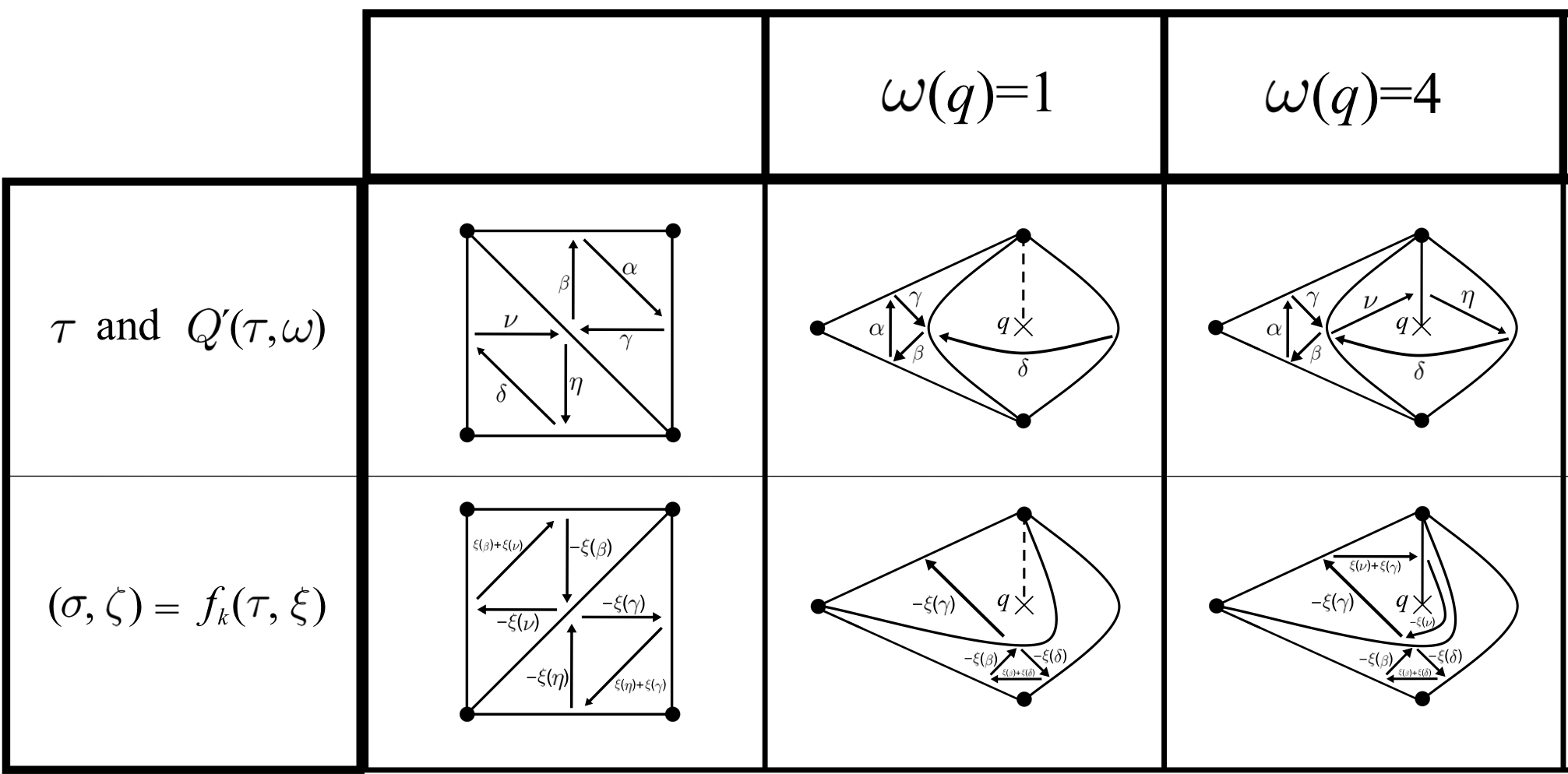
Figure 9.

In the bottom row of each table we see the effect that the colored flip of $k$ has on $(\tau,\xi)$ for any 1-cocycle $\xi\in Z^{1}(\tau,\omega)$ (in the top row, the arrows are labeled by their names, while in the bottom row the arrows are labeled by the corresponding values of $\zeta$, where $\zeta\in Z^{1}(\sigma,\omega)$ is the underlying 1-cocycle of the colored triangulation $(\sigma,\zeta):=f_{k}(\tau,\xi)$; the values of $\zeta$ are written in terms of the values of $\xi$).

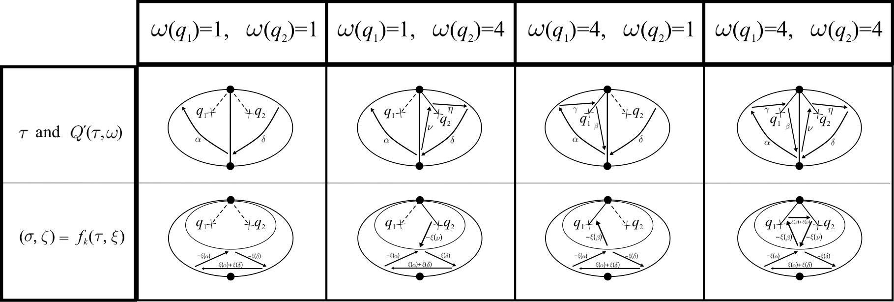
Figure 10.

In this example we can glimpse a general fact which is actually easy to prove, namely, that if $k$ is non-pending, then the function $Z^{1}(\tau,\omega)\rightarrow Z^{1}(\sigma,\omega)$, $\xi\mapsto\zeta$, is linear.

Example 5.10.

Figure 11 depicts a table. In the top row of the table we can see a puzzle piece, with the corresponding portion of the quiver $Q^{\prime}(\tau,\omega)$ drawn on it for all the possible values of $\omega$ at the orbifold points contained in the puzzle piece respectively involved.

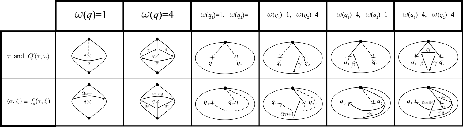
Figure 11.

In the bottom row of the table we can again see the effect that flipping $k$ has on $(\tau,\xi)$ for any 1-cocycle $\xi\in Z^{1}(\tau,\omega)$ (as before, the arrows in the top row are labeled with their names, while in the bottom row the arrows are labeled by the corresponding values of $\zeta$, where $\zeta\in Z^{1}(\sigma,\omega)$ is the underlying 1-cocycle of the colored triangulation $(\sigma,\zeta):=f_{k}(\tau,\xi)$; the values of $\zeta$ are again written in terms of the values of $\xi$).

In this example we can glimpse a general fact which is in fact easy to prove, namely, that if $k$ is pending and $d(\tau,\omega)_{k}=4$, then the function $Z^{1}(\tau,\omega)\rightarrow Z^{1}(\sigma,\omega)$, $\xi\mapsto\zeta$, is linear. Furthermore, if $k$ is pending and $d(\tau,\omega)_{k}=1$, then the function $Z^{1}(\tau,\omega)\rightarrow Z^{1}(\sigma,\omega)$, $\xi\mapsto\zeta$, may fail to be linear.

6. The species with potential of a colored triangulation

In this section we associate a species with potential to each colored triangulation of a surface with weighted orbifold points. The reader is kindly asked to recall from Definition 5.1 that a colored triangulation is a pair $(\tau,\xi)$ consisting of a triangulation $\tau$ and a choice of a 1-cocycle $\xi\in{Z^{1}({\tau,\omega})}\subseteq{C^{1}({\tau,\omega})}=\operatorname{Hom}_{\mathbb{F}_{2}}({C_{1}({\tau,\omega})},\mathbb{F}_{2})$. According to Definition 3.3, the pair $(\tau,\omega)$ dictates us a weighted quiver $(Q(\tau,\omega),\mathbf{d}(\tau,\omega))$. The 1-cocycle $\xi$ will dictate us a modulating function $g(\tau,\xi)$ for this weighted quiver (see [27, Definition 3.2] for the definition of what a modulating function is). This means in particular that we will not be working with arbitrary modulating functions on $(Q(\tau,\omega),\mathbf{d}(\tau,\omega))$, but only with those defined by 1-cocycles; the reason for this is that only the modulating functions arising from 1-cocycles have the chance of producing species admitting non-degenerate potentials, as will become clear in the proof of our main result (Theorem 7.1) and in Section 11 (see Lemma 11.1 and Corollary 11.4).

6.1. The species

Let $(\tau,\xi)$ be a colored triangulation of ${\mathbf{\Sigma}_{\omega}}=(\Sigma,\mathbb{M},\mathbb{O},\omega)$. Set $d=\operatorname{lcm}(d(\tau,\omega)_{k}\ |\ k\in\tau)\in\{2,4\}$, let $F$ be a field containing a primitive $d^{\operatorname{th}}$ root of unity, and let $E/F$ be a degree-$d$ cyclic Galois field extension. Following [27, Equation (3.4)], once and for all we fix an element $v\in E$ with the property that $\{v^{\ell}\ |\ \ell\in\{0,1,\ldots,v^{d-1}\}\}$ is an eigenbasis of $E/F$.

The degree $[E:F]=d$ is $2$ or $4$. In any case, $E$ always contains a unique field extension $L$ of $F$ such that $[L:F]=2$. Once and for all, we fix an element $u\in L$ with the property that $\{1,u\}$ is an eigenbasis of $L/F$. We always can, and will, assume that

$$u=\begin{cases}v^{2}&\text{if $d=4$;}\\ v&\text{if $d=2$}.\end{cases}$$

We will denote by $\theta$ the unique non-identity element of $\operatorname{Gal}(L/F)$, so that $\operatorname{Gal}(L/F)=\{11_{L},\theta\}$. If $[E:F]=4$, then $\operatorname{Gal}(E/F)$ is a cyclic group with four elements, and we fix a generator $\rho$ once and for all. This generator necessarily satisfies $11_{E}|_{L}=11_{L}=\rho^{2}|_{L}$ and $\rho|_{L}=\theta=\rho^{3}|_{L}$.

For each $k\in\tau$ we set $F_{k}/F$ to be the unique degree-$d(\tau,\omega)_{k}$ field subextension of $E/F$, and denote $G_{k}=\operatorname{Gal}(F_{k}/F)$. We also denote $G_{j,k}=\operatorname{Gal}(F_{j}\cap F_{k}/F)$ for $i,j\in\tau$. Thus:

$$G_{k}=\begin{cases}\{11_{F_{k}},\rho,\rho^{2},\rho^{3}\}&\text{if $[F_{k}:F]=4$;}\\ \{11_{F_{k}},\theta\}&\text{if $[F_{k}:F]=2$;}\\ \{11_{F_{k}}\}&\text{if $[F_{k}:F]=1$.}\end{cases}$$

Definition 6.1.

Let $(\tau,\xi)$ be a colored triangulation of ${\mathbf{\Sigma}_{\omega}}$. We define a modulating function $g(\tau,\xi):Q(\tau,\omega)_{1}\rightarrow\bigcup_{j,k\in\tau}G_{j,k}$ as follows. Take $\alpha\in Q(\tau,\xi)_{1}$.

1. If $d(\tau,\omega)_{h(\alpha)}=1$ or $d(\tau,\omega)_{t(\alpha)}=1$, set

   $$g(\tau,\xi)_{\alpha}=11_{F_{h(\alpha),t(\alpha)}}\in G_{h(\alpha),t(\alpha)}.$$

2. If $d(\tau,\omega)_{h(\alpha)}\neq 1\neq d(\tau,\omega)_{t(\alpha)}$, and $d(\tau,\omega)_{h(\alpha)}d(\tau,\omega)_{t(\alpha)}<16$, set

   $$g(\tau,\xi)_{\alpha}=\theta^{\xi(\alpha)}\in\ G_{h(\alpha),t(\alpha)}.$$

3. If $d(\tau,\omega)_{h(\alpha)}=4=d(\tau,\omega)_{t(\alpha)}$, then

   1. $t(\alpha)$ and $h(\alpha)$ are pending arcs contained in a twice orbifolded triangle $\triangle$, and the quiver $Q^{\prime}(\tau,\omega)$ has exactly one arrow $t(\alpha)\rightarrow h(\alpha)$, induced by $\triangle$; let $\delta_{0}^{\triangle}$ be this arrow of $Q^{\prime}(\tau,\omega)$; notice that we can evaluate $\xi$ at $\delta_{0}^{\triangle}$;

   2. the quiver $Q(\tau,\omega)$ has exactly two arrows going from $t(\alpha)$ to $h(\alpha)$, one of which is $\delta_{0}^{\triangle}$; let $\delta_{1}^{\triangle}$ be the other such arrow of $Q(\tau,\omega)$; of course, $\alpha\in\{\delta_{0}^{\triangle},\delta_{1}^{\triangle}\}$;

   3. $[E:F]=4$ and $F_{h(\alpha)}=E=F_{t(\alpha)}$; let $\ell$ be the unique element of $\{0,1\}$ whose residue class modulo 2 is $\xi(\delta_{0}^{\triangle})\in\mathbb{F}_{2}=\mathbb{Z}/2\mathbb{Z}$ (equivalently, let $\ell$ be the unique element of $\{0,1\}$ such that $\rho^{\ell}|_{L}=\theta^{\xi(\delta_{0}^{\triangle})}=\rho^{\ell+2}|_{L}$).

   We set

   $$g(\tau,\xi)_{\alpha}=\begin{cases}\rho^{\ell}&\text{if $\alpha=\delta_{0}^{\triangle}$;}\\ \rho^{\ell+2}&\text{if $\alpha=\delta_{1}^{\triangle}$.}\end{cases}$$

Definition 6.2.

The species over $E/F$ of the colored triangulation $(\tau,\xi)$ is the species of the triple $(Q(\tau,\omega),\mathbf{d}(\tau,\omega),g(\tau,\xi))$ (cf. [27]). We shall denote it by $A(\tau,\xi)$.

For the next two examples, let $p$ be a positive prime number congruent to 1 modulo $4$ (e.g. $p=5$), and let $F$ be the field with $p$ elements. Let $z\in F$ be an element which is not a square in $F$ (e.g. $z=2$ if $p=5$, or, more generally, $z=2$ if $p^{2}\not\equiv 1\ \operatorname{mod}16$). Then the polynomial $X^{4}-z$ is irreducible over $F$ (see for example [12, Theorem 5.4.1]), which means that if $E$ is the field with $p^{4}$ elements, then there exists an element $v\in E$ such that $v^{4}=z$ and $E=F(v)$. Letting $\rho:E\rightarrow E$ be the Frobenius automorphism of the extension $E/F$, and writing $p=4q+1$ (e.g. $5=4\cdot 1+1$), we have $\rho(v)=v^{p}=v^{4q+1}=z^{q}v$ (e.g. $\rho(v)=v^{5}=2v$ if $p=5$ or, more generally, if $p^{2}\not\equiv 1\ \operatorname{mod}16$), which means that $\{1,v,v^{2},v^{3}\}$ is an eigenbasis of $E/F$.

Example 6.3.

Let $(\Sigma,\mathbb{M},\mathbb{O})$ be an unpunctured hexagon with one orbifold point, and let $\omega:\mathbb{O}\rightarrow\{1,4\}$ be the function that takes the value 4 at the only element of $\mathbb{O}$.

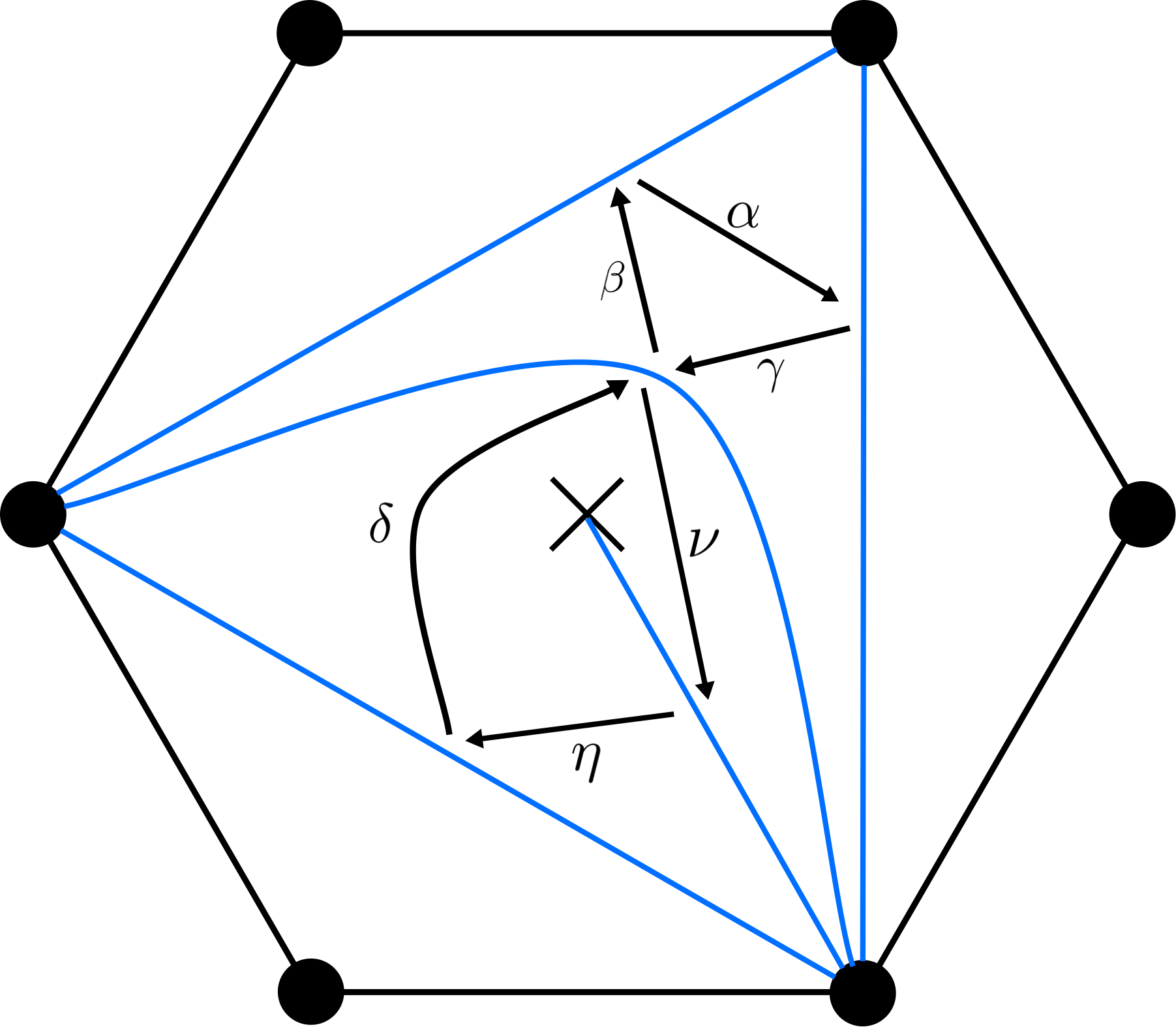
Figure 12. .

In Figure 12, the reader can see a triangulation $\tau$ of $(\Sigma,\mathbb{M},\mathbb{O})$ and the quiver $Q^{\prime}(\tau,\omega)$, which in this particular example coincides with $Q(\tau,\omega)$. For any cocycle $\xi\in Z^{1}(\tau,\omega)$, the following identities hold in the (complete) path algebra of the corresponding species $A(\tau,\xi)$:

$\alpha\beta\gamma v^{2}=v^{2}\alpha\beta\gamma$,

$\nu\delta\eta v^{2}=v^{2}\nu\delta\eta$.

Example 6.4.

Let $(\Sigma,\mathbb{M},\mathbb{O})$ be an unpunctured pentagon with two orbifold points, and let $\omega:\mathbb{O}\rightarrow\{1,4\}$ be the function that takes the value 4 at both elements of $\mathbb{O}$.

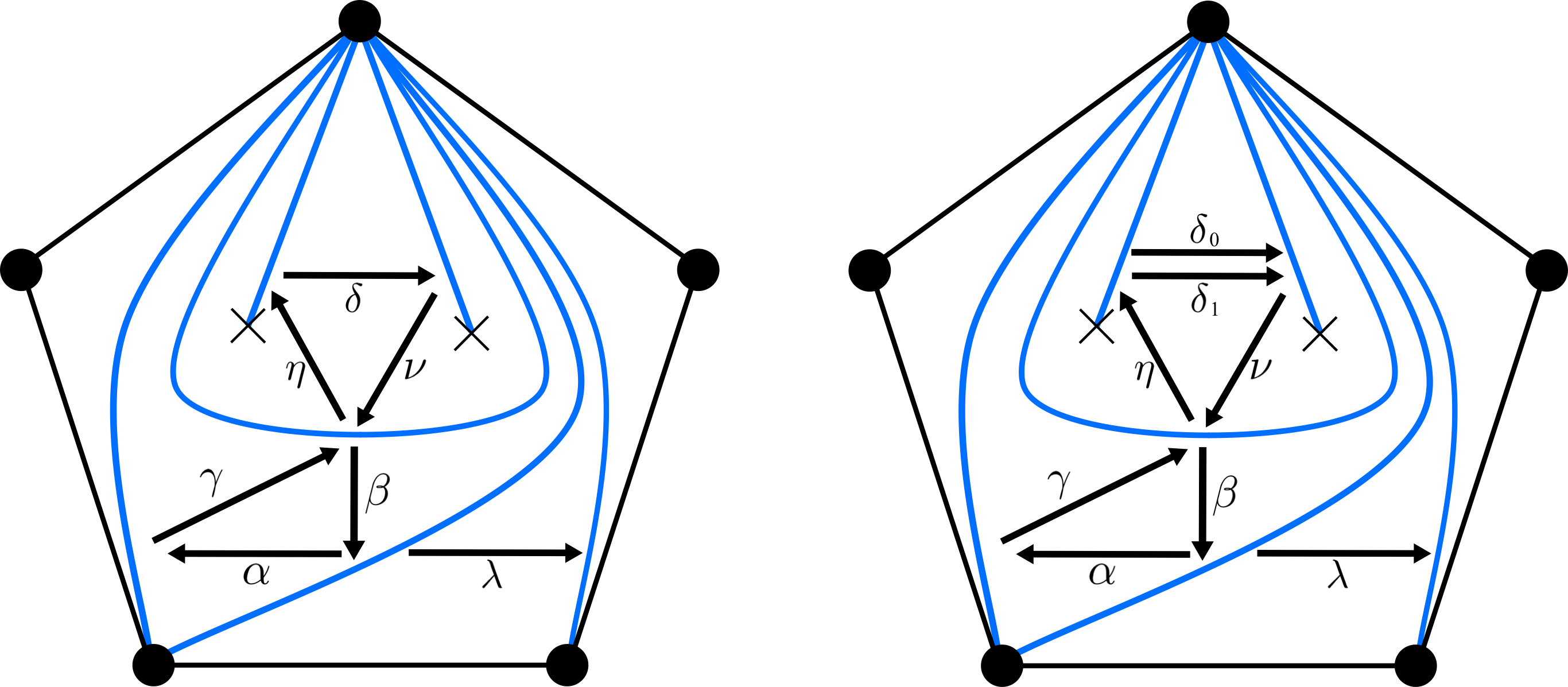
Figure 13. .

In Figure 13, the reader can see a triangulation $\tau$ of $(\Sigma,\mathbb{M},\mathbb{O})$ and the quivers $Q^{\prime}(\tau,\omega)$ (left) and $Q(\tau,\omega)$ (right), which in this example do not coincide. For any cocycle $\xi\in Z^{1}(\tau,\omega)$, the following identities hold in the (complete) path algebra of the corresponding species $A(\tau,\xi)$:

$\delta_{0}\eta\nu v^{2}=v^{2}\delta_{0}\eta\nu$,

$\delta_{1}\eta\nu v^{2}=v^{2}\delta_{1}\eta\nu$,

$\delta_{0}v=z^{\ell q}v\delta_{0}$, $\delta_{1}v=z^{(\ell+2)q}v\delta_{1}$,

where $\ell$ is defined as the unique element of $\{0,1\}\subseteq\mathbb{Z}$ whose class modulo $2$ is $\xi(\delta)\in\mathbb{F}_{2}=\mathbb{Z}/2\mathbb{Z}$. For instance, if $p=5$, $z=2$ and $\xi(\delta)=0$, then $\delta_{0}v=v\delta_{0}$, and $\delta_{1}v=4v\delta_{1}$, whereas if $p=5$, $z=2$ and $\xi(\delta)=1$, then $\delta_{0}v=2v\delta_{0}$, and $\delta_{1}v=8v\delta_{1}$

We leave the easy proof of the following two results in the hands of the reader.

Proposition 6.5.

Let ${\mathbf{\Sigma}}=(\Sigma,\mathbb{M},\mathbb{O})$ be a surface as in Section 2 and $(\tau,\omega)$ be any pair consisting of a triangulation $\tau$ of ${\mathbf{\Sigma}}$ and a function $\omega:\mathbb{O}\rightarrow\{1,4\}$. Let $B(\tau,\omega)=(b_{kj}(\tau,\omega))_{k,j}$ be the skew-symmetrizable matrix that corresponds to the weighted quiver $(Q(\tau,\omega),\mathbf{d}(\tau,\omega))$ under [32, Lemma 2.3] (that is, the matrix associated to $(\tau,w)$ by Felikson-Shapiro-Tumarkin, where $w(q)=\frac{2}{\omega(q)}$ for $q\in\mathbb{O}$, see Remark 3.5-(2)). For any 1-cocycle $\xi\in Z^{1}(\tau,\omega)$, the pair $(\mathbf{F},\mathbf{A})$ is a species realization of $B(\tau,\omega)$ (cf. [27, Definition 2.22]), where $\mathbf{F}=(F_{k})_{k\in\tau}$ and $\mathbf{A}=(e_{k}A(\tau,\xi)e_{j})_{k,j\in\tau}$ ($e_{j}$ being the idempotent element of $R:=\bigoplus_{k\in\tau}F_{k}$ that has a $1$ in its $j^{\operatorname{th}}$ entry and zeros elsewhere). More precisely, $\mathbf{F}$ is a tuple of division rings and for every pair $(k,j)\in\tau\times\tau$ such that $b_{kj}(\tau,\omega)\geq 0$ we have that:

1. $e_{k}A(\tau,\xi)e_{j}$ is an $F_{k}$-$F_{j}$-bimodule;

2. $\dim_{F_{k}}(e_{k}A(\tau,\xi)e_{j})=b_{kj}(\tau,\omega)$ and $\dim_{F_{j}}(e_{k}A(\tau,\xi)e_{j})=-b_{jk}(\tau,\omega)$;

3. $\operatorname{Hom}_{F_{k}}(e_{k}A(\tau,\xi)e_{j},F_{k})$ and $\operatorname{Hom}_{F_{j}}(e_{k}A(\tau,\xi)e_{j},F_{j})$ are isomorphic as $F_{j}$-$F_{k}$-bimodules.

Proposition 6.6.

Let ${\mathbf{\Sigma}}=(\Sigma,\mathbb{M},\mathbb{O})$ be a surface as in Section 2, $\omega:\mathbb{O}\rightarrow\{1,4\}$ a function, $(\tau,\xi)$ a colored triangulation of ${\mathbf{\Sigma}_{\omega}}$, and $k\in\tau$. If $W\in R\langle\langle A(\tau,\xi)\rangle\rangle$ is a potential such that the SP $(A^{\prime},W^{\prime}):=\mu_{k}(A(\tau,\xi),W)$ is 2-acyclic, then $A^{\prime}\cong A(f(\tau,\xi))$ as $R$-$R$-bimodules.

6.2. The potential

Definition 6.7.

(Cycles from non-orbifolded triangles). Let $(\tau,\xi)$ be a colored triangulation of ${\mathbf{\Sigma}_{\omega}}$ and $\triangle$ be an interior triangle of $\tau$ not containing any orbifold point. Then there is a 3-cycle $\alpha^{\triangle}\beta^{\triangle}\gamma^{\triangle}$ on $Q(\tau,\omega)$ formed with the arrows $\alpha^{\triangle},\beta^{\triangle},\gamma^{\triangle}$ contained in $\triangle$ (see the picture on the upper left in Figure 14). We set $S^{\triangle}(\tau,\xi)=\alpha^{\triangle}\beta^{\triangle}\gamma^{\triangle}$.

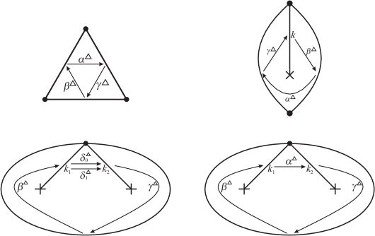
Figure 14. Notation for the definition of $S(\tau,\xi)$.

Definition 6.8.

(Cycles from triangles with exactly one orbifold point). Let $(\tau,\xi)$ be a colored triangulation of ${\mathbf{\Sigma}_{\omega}}$ and $\triangle$ be an interior triangle of $\tau$ containing exactly one orbifold point. Let $k$ be the unique pending arc of $\tau$ contained in $\triangle$. Using the notation from the picture on the upper right in Figure 14, we set $S^{\triangle}(\tau,\xi)=\alpha^{\triangle}\beta^{\triangle}\gamma^{\triangle}$, regardless of whether $d(\tau,\omega)_{k}=1$ or $d(\tau,\omega)_{k}=4$.

Definition 6.9 (Cycles from triangles with exactly two orbifold points).

Let $(\tau,\xi)$ be a colored triangulation of ${\mathbf{\Sigma}_{\omega}}$ and $\triangle$ be an interior triangle of $\tau$ containing exactly two orbifold points. Let $k_{1}$ and $k_{2}$ be the two pending arcs of $\tau$ contained in $\triangle$, and assume that $Q(\tau,\omega)$ has (at least) one arrow going from $k_{1}$ to $k_{2}$.

• If $d(\tau,\omega)_{k_{1}}=1=d(\tau,\omega)_{k_{2}}$, then, with the notation of the picture on the bottom left in Figure 14, we set $S^{\triangle}(\tau,\xi)=\delta_{0}^{\triangle}\beta^{\triangle}\gamma^{\triangle}+\delta_{1}^{\triangle}\beta^{\triangle}u\gamma^{\triangle}$.

• If $d(\tau,\omega)_{k_{1}}=1$ and $d(\tau,\omega)_{k_{2}}=4$, then, with the notation of the picture on the bottom right in Figure 14, we set $S^{\triangle}(\tau,\xi)=\alpha^{\triangle}\beta^{\triangle}\gamma^{\triangle}$.

• If $d(\tau,\omega)_{k_{1}}=4$ and $d(\tau,\omega)_{k_{2}}=1$, then, with the notation of the picture on the bottom right in Figure 14, we set $S^{\triangle}(\tau,\xi)=\alpha^{\triangle}\beta^{\triangle}\gamma^{\triangle}$.

• If $d(\tau,\omega)_{k_{1}}=4$ and $d(\tau,\omega)_{k_{2}}=4$, then, with the notation of the picture on the bottom left in Figure 14, we set $S^{\triangle}(\tau,\xi)=(\delta_{0}^{\triangle}+\delta_{1}^{\triangle})\beta^{\triangle}\gamma^{\triangle}$.

Definition 6.10 (The potential of a colored triangulation).

Let ${\mathbf{\Sigma}}=(\Sigma,\mathbb{M},\mathbb{O})$ be an unpunctured surface with marked points and orbifold points of order 2, $\omega:\mathbb{O}\rightarrow\{1,4\}$ any function, and $(\tau,\xi)$ a colored triangulation of ${\mathbf{\Sigma}_{\omega}}=(\Sigma,\mathbb{M},\mathbb{O},\omega)$. The potential associated to $(\tau,\xi)$ is

$$S(\tau,\xi)=\sum_{\triangle}S^{\triangle}(\tau,\xi)\in R\langle A(\tau,\xi)\rangle\subseteq R\langle\langle A(\tau,\xi)\rangle\rangle,$$

where the sum runs over all interior triangles of $\tau$.

Example 6.11.

Let ${\mathbf{\Sigma}_{\omega}}=(\Sigma,\mathbb{M},\mathbb{O},\omega)$ and $\tau$ be as in Example 6.3. For any 1-cocycle $\xi\in Z^{1}(\tau,\omega)$, the potential $S(\tau,\xi)$ is

$$S(\tau,\xi)=\alpha\beta\gamma+\delta\eta\nu,$$

whose cyclic derivatives are (see [27, Definition 3.11] for the definition of cyclic derivative)

$\partial_{\alpha}(S(\tau,\xi))=\pi_{g(\tau,\xi)_{\alpha}^{-1}}\left(\beta\gamma\right)=\beta\gamma$,	$\partial_{\beta}(S(\tau,\xi))=\pi_{g(\tau,\xi)_{\beta}^{-1}}\left(\gamma\alpha\right)=\gamma\alpha$,	$\partial_{\gamma}(S(\tau,\xi))=\pi_{g(\tau,\xi)_{\gamma}^{-1}}\left(\alpha\beta\right)=\alpha\beta$,
$\partial_{\delta}(S(\tau,\xi))=\pi_{g(\tau,\xi)_{\delta}^{-1}}\left(\eta\nu\right)=\eta\nu$,	$\partial_{\eta}(S(\tau,\xi))=\pi_{g(\tau,\xi)_{\eta}^{-1}}\left(\nu\delta\right)=\nu\delta$,	$\partial_{\nu}(S(\tau,\xi))=\pi_{g(\tau,\xi)_{\nu}^{-1}}\left(\delta\eta\right)=\delta\eta$,

where $\pi_{\rho}(x)=\frac{1}{2}\left(x+\rho(v^{-2})xv^{2}\right)$ for $\rho\in\operatorname{Gal}(L/F)$. Thus, the following identities hold in the Jacobian algebra $\mathcal{P}(A(\tau,\xi),S(\tau,\xi))$ besides the ones listed in Example 6.3 (see [27, Definition 3.11] for the definition of the Jacobian algebra of an SP):

$$\alpha\beta=\beta\gamma=\gamma\alpha=\delta\eta=\eta\nu=\nu\delta=0,$$

from which it easily follows that $\dim_{F}(\mathcal{P}(A(\tau,\xi),S(\tau,\xi)))<\infty$. Note, however, that $\eta v\nu\neq 0$ in $\mathcal{P}(A(\tau,\xi),S(\tau,\xi))$.

Example 6.12.

Let ${\mathbf{\Sigma}_{\omega}}=(\Sigma,\mathbb{M},\mathbb{O},\omega)$ and $\tau$ be as in Example 6.4. For any 1-cocycle $\xi\in Z^{1}(\tau,\omega)$, the potential $S(\tau,\xi)$ is

$$S(\tau,\xi)=\alpha\beta\gamma+(\delta_{0}+\delta_{1})\eta\nu,$$

whose cyclic derivatives are

$\partial_{\alpha}(S(\tau,\xi))=\beta\gamma$,

$\partial_{\beta}(S(\tau,\xi))=\gamma\alpha$,

$\partial_{\gamma}(S(\tau,\xi))=\alpha\beta$,

$\partial_{\delta_{0}}(S(\tau,\xi))=\pi_{g(\tau,\xi)_{\delta_{0}}^{-1}}\left(\eta\nu\right)=\frac{1}{2}\left(\eta\nu+g(\tau,\xi)_{\delta_{0}}^{-1}(v^{-1})\eta\nu v\right)$,

$\partial_{\delta_{1}}(S(\tau,\xi))=\pi_{g(\tau,\xi)_{\delta_{1}}^{-1}}\left(\eta\nu\right)=\frac{1}{2}\left(\eta\nu+g(\tau,\xi)_{\delta_{1}}^{-1}(v^{-1})\eta\nu v\right)$,

$\partial_{\eta}(S(\tau,\xi))=\frac{1}{2}\left(\nu\delta_{0}+g(\tau,\xi)_{\eta}^{-1}(v^{-2})\nu\delta_{0}v^{2}\right)+\frac{1}{2}\left(\nu\delta_{1}+g(\tau,\xi)_{\eta}^{-1}(v^{-2})\nu\delta_{1}v^{2}\right)=\nu\delta_{0}+\nu\delta_{1}$,

$\partial_{\nu}(S(\tau,\xi))=\frac{1}{2}\left(\delta_{0}\eta+g(\tau,\xi)_{\nu}^{-1}(v^{-2})\delta_{0}\eta v^{2}\right)+\frac{1}{2}\left(\delta_{1}\eta+g(\tau,\xi)_{\nu}^{-1}(v^{-2})\delta_{1}\eta v^{2}\right)=\delta_{0}\eta+\delta_{1}\eta$,

where $\pi_{\rho}(x)=\frac{1}{4}\left(x+\rho(v^{-1})xv+\rho(v^{-2})xv^{2}+\rho(v^{-3})xv^{3}\right)$ for $\rho\in\operatorname{Gal}(E/F)$. Thus, the following identities hold in the Jacobian algebra $\mathcal{P}(A(\tau,\xi),S(\tau,\xi))$ besides the ones listed in Example 6.4:

$$\alpha\beta=\beta\gamma=\gamma\alpha=\eta\nu=\nu\delta_{0}+\nu\delta_{1}=\delta_{0}\eta+\delta_{1}\eta=0,$$

from which it easily follows that $\dim_{F}(\mathcal{P}(A(\tau,\xi),S(\tau,\xi)))<\infty$.

7. Flip is compatible with SP-mutation

Here we present the main result of this paper, which says that whenever two colored triangulations are related by the flip of an arc, then their associated SPs are related by the SP-mutation defined in [27, Definitions 3.19 and 3.22]. The precise statement is:

Theorem 7.1.

Let ${\mathbf{\Sigma}}=(\Sigma,\mathbb{M},\mathbb{O})$ be either an unpunctured surface with marked points and order-2 orbifold points, or a once-punctured closed surface with order-2 orbifold points; let $\omega:\mathbb{O}\rightarrow\{1,4\}$ be any function, and let $(\tau,\xi)$ and $(\sigma,\zeta)$ be colored triangulations of ${\mathbf{\Sigma}_{\omega}}=(\Sigma,\mathbb{M},\mathbb{O},\omega)$. If $(\sigma,\zeta)$ is obtained from $(\tau,\xi)$ by the colored flip of an arc $k\in\tau$, then the SPs $(A(\sigma,\zeta),S(\tau,\zeta))$ and $\mu_{k}(A(\tau,\xi),S(\tau,\xi))$ are right-equivalent.

The proof we give of this theorem is rather long as we achieve it by verifying that its statement is true for all the possible configurations that $\tau$ can present locally around the arc $k$. As such, the proof, which the reader can find in Section 14, is done case by case. Worth mentioning is the fact that in many of these cases it will be crucial that $A(\tau,\xi)$ and $A(\sigma,\zeta)$ are given by Definitions 6.1 and 6.2, and that $S(\tau,\xi)$ and $S(\sigma,\zeta)$ are given by Definitions 6.7, 6.8, 6.9 and 6.10.

Notice that Theorem 7.1 immediately implies:

Corollary 7.2.

For ${\mathbf{\Sigma}_{\omega}}$ as in the statement of Theorem 7.1, the species with potential associated to its colored triangulations are non-degenerate in the sense of Derksen-Weyman-Zelevinsky (cf. [14, Definition 7.2]).

8. Geometric realization of the complexes ${C_{\bullet}({\tau,\omega})}$ and ${\widehat{C}_{\bullet}({\tau,\omega})}$

Recall that the surfaces $(\Sigma,\mathbb{M},\mathbb{O})$ we are working with in this paper have an arbitrary number of orbifold points, and are either unpunctured with non-empty boundary, or closed with exactly one puncture. Set

(8.1) $$\widetilde{\Sigma} = \begin{cases}\Sigma&\text{if $\Sigma$ has non-empty boundary;}\\ \Sigma\setminus\mathbb{M}&\text{if $\Sigma$ has empty boundary.}\end{cases}$$

We will show that the homology ${H_{\bullet}(C_{\bullet}({\tau,\omega}))}$ is isomorphic to the singular homology $H_{\bullet}(\widetilde{\Sigma};\mathbb{F}_{2})$ of $\widetilde{\Sigma}$ and ${H_{\bullet}(\widehat{C}_{\bullet}({\tau,\omega}))}$ to the singular homology $H_{\bullet}(\widehat{\Sigma};\mathbb{F}_{2})$ of $\widehat{\Sigma}=\widetilde{\Sigma}\setminus\{q\in\mathbb{O}\ |\ \omega(q)=1\}$. See [4, Lemma 2.3], [5, Proposition 3.4], [7] or [34] for similar results established before. It will be important for the next section of this paper that the isomorphisms are induced by the inclusions of specific “geometric realizations” of $X_{\bullet}({\tau,\omega})$ and $\widehat{X}_{\bullet}({\tau,\omega})$ as topological subspaces of $\widetilde{\Sigma}$ and $\widehat{\Sigma}$, respectively.

Remark 8.1.

If $(\Sigma,\mathbb{M},\mathbb{O})$ is an unpunctured surface, then $\widehat{\Sigma}$ can be interpreted as the associated triangulated orbifold $\widehat{\mathcal{O}}=\widehat{\mathcal{O}}({\tau,\omega})$ described in [18, Definition 5.10].

To argue that the homology of the chain complexes ${C_{\bullet}({\tau,\omega})}$ and ${\widehat{C}_{\bullet}({\tau,\omega})}$ can be canonically identified with the singular homology of the surfaces $\widetilde{\Sigma}$ and $\widehat{\Sigma}$ with $\mathbb{F}_{2}$-coefficients, respectively, it is convenient to construct two topological subspaces $Y({\tau,\omega})\subseteq\widehat{Y}({\tau,\omega})$ of $\Sigma$. These subspaces should be regarded as “geometric realizations” of $X_{\bullet}({\tau,\omega})$ and $\widehat{X}_{\bullet}({\tau,\omega})$, respectively. To obtain the spaces $Y({\tau,\omega})\subseteq\widehat{Y}({\tau,\omega})$ we proceed as follows:

1. For each arc $i\in X_{0}({\tau,\omega})=\tau\setminus\tau^{\omega=1}$ choose a point $y_{i}$ in the interior of $i$.

2. For each ${{\alpha}}\in\widehat{X}_{1}({\tau,\omega})$ choose a simple curve $c_{{{\alpha}}}$ going from $y_{t(\alpha)}$ to $y_{h(\alpha)}$ inside the triangle $\triangle$ containing $\alpha$. If $\alpha=\varepsilon^{\tau}_{k}$ for some $k\in\tau^{\omega=1}$, let $c_{{{\alpha}}}$ be chosen in such a way that it crosses $k$ exactly once, and that such crossing happens in a non-endpoint of $k$. Otherwise, the interior of $c_{{{\alpha}}}$ should not intersect any arc of $\tau$. Moreover, we assume that the interior of $c_{{{\alpha}}}$ intersects neither the boundary of $\triangle$ nor any $c_{{{\beta}}}$ with ${{\beta}}\neq{{\alpha}}$.

3. Observe that for each triangle $\triangle\in X_{2}({\tau,\omega})$ the set $c_{\triangle}=\bigcup_{\text{$\alpha$ induced by $\triangle$}}c_{{{\alpha}}}$ is a closed simple curve in $\Sigma$. Let $f_{\triangle}$ be the closure of the connected component of $\Sigma\setminus c_{\triangle}$ not intersecting any arc of $\tau$.

4. We define

   $$Y({\tau,\omega})\>=\>\bigcup_{i\in X_{0}({\tau,\omega})}\{y_{i}\}\>\>\cup\>\>\bigcup_{{{\alpha}}\in X_{1}({\tau,\omega})}c_{{{\alpha}}}\>\>\cup\>\>\bigcup_{\triangle\in X_{2}({\tau,\omega})}f_{\triangle}$$

   and

   $$\widehat{Y}({\tau,\omega})\>=\>\bigcup_{i\in\widehat{X}_{0}({\tau,\omega})}\{y_{i}\}\>\>\cup\>\>\bigcup_{{{\alpha}}\in\widehat{X}_{1}({\tau,\omega})}c_{{{\alpha}}}\>\>\cup\>\>\bigcup_{\triangle\in\widehat{X}_{2}({\tau,\omega})}f_{\triangle}\,.$$

Example 8.2.

Consider the triangulations $\tau$ and $\sigma$ of the unpunctured pentagon with two orbifold points depicted in Figure 4. In Figures 5 and 6 we can see the topological subspace $\widehat{Y}({\tau,\omega})$ of $\Sigma$ depicted for every choice of function $\omega:\mathbb{O}\{1,4\}$.

To relate the homology of ${C_{\bullet}({\tau,\omega})}$ and ${\widehat{C}_{\bullet}({\tau,\omega})}$ to the singular homology of $Y({\tau,\omega})$ and $\widehat{Y}({\tau,\omega})$ we fix:

• for each $i\in\widehat{X}_{0}({\tau,\omega})$, the function $\theta_{i}:\Delta^{0}\rightarrow\widehat{\Sigma}$ taking value $y_{i}$, where $\Delta^{0}=\{\star\}$ is the 0-simplex;

• for each ${{\alpha}}\in\widehat{X}_{1}({\tau,\omega})$, a parametrization $\theta_{{{\alpha}}}:\Delta^{1}\to\widehat{\Sigma}$ of $c_{{{\alpha}}}$, where $\Delta^{1}\cong[0,1]$ is the 1-simplex, such that the restriction of $\theta_{{{\alpha}}}$ to the interior of $\Delta^{1}$ is injective, $\theta_{{{\alpha}}}(0)=y_{t(\alpha)}$, and $\theta_{{{\alpha}}}(1)=y_{h(\alpha)}$; and

• for each $\triangle\in\widehat{X}_{2}({\tau,\omega})$, a parametrization $\theta_{\triangle}:\Delta^{2}\to\widehat{\Sigma}$ of $f_{\triangle}$, where $\Delta^{2}$ is the 2-simplex, such that the restriction of $\theta_{\triangle}$ to the interior of $\Delta^{2}$ is injective and any restriction of $\theta_{\triangle}$ to a face of $\Delta^{2}$ parametrizes one of the curves $c_{{{\alpha}}}$ for some $\alpha\in X_{1}({\tau,\omega})$ induced by $\triangle$.

We use the notation $C_{\bullet}(\widehat{Y}({\tau,\omega});\mathbb{F}_{2})$ for the singular complex with coefficients in $\mathbb{F}_{2}$ of the topological space $\widehat{Y}({\tau,\omega})$. The following is a standard result in basic algebraic topology.

Proposition 8.3.

The map of chain complexes ${\widehat{C}_{\bullet}({\tau,\omega})}\to C_{\bullet}(\widehat{Y}({\tau,\omega});\mathbb{F}_{2})$ that maps $x\in\coprod_{n\in\mathbb{N}}\widehat{X}_{n}({\tau,\omega})$ to $\theta_{x}$ induces isomorphisms ${H_{\bullet}(\widehat{C}_{\bullet}({\tau,\omega}))}\to H_{\bullet}(\widehat{Y}({\tau,\omega});\mathbb{F}_{2})$ and ${H_{\bullet}(C_{\bullet}({\tau,\omega}))}\to H_{\bullet}(Y({\tau,\omega});\mathbb{F}_{2})$.

Remark 8.4.

A result similar to Proposition 8.3 also holds when taking coefficients in $\mathbb{Z}$ instead of $\mathbb{F}_{2}$. However, one has to be a little bit more careful with the choice of the $\theta_{x}$ in this case, since $-1\neq 1$ in $\mathbb{Z}$.

The next proposition tells us together with Proposition 8.3 that, as claimed earlier, we have quasi-isomorphisms ${C_{\bullet}({\tau,\omega})}\to C_{\bullet}(\Sigma;\mathbb{F}_{2})$ and ${\widehat{C}_{\bullet}({\tau,\omega})}\to C_{\bullet}(\widehat{\Sigma};\mathbb{F}_{2})$.

Proposition 8.5.

The canonical inclusions $\iota:Y({\tau,\omega})\to\widetilde{\Sigma}$ and $\widehat{\iota}:\widehat{Y}({\tau,\omega})\to\widehat{\Sigma}$ induce isomorphisms in homology $\iota_{*}:H_{\bullet}(Y({\tau,\omega});\mathbb{F}_{2})\to H_{\bullet}(\widetilde{\Sigma};\mathbb{F}_{2})$ and $\widehat{\iota}_{*}:H_{\bullet}(\widehat{Y}({\tau,\omega});\mathbb{F}_{2})\to H_{\bullet}(\widehat{\Sigma};\mathbb{F}_{2})$.

Remark 8.6.

Proposition 8.5 follows from the observation that $Y({\tau,\omega})$ is a strong deformation retract of $\widetilde{\Sigma}$ and $\widehat{Y}({\tau,\omega})$ a strong deformation retract of $\widehat{\Sigma}$. We give a proof requiring less imagination.

Proof of Proposition 8.5.

Clearly, $H_{0}(Y({\tau,\omega});\mathbb{F}_{2})$ has dimension $1$ and $H_{n}(Y({\tau,\omega});\mathbb{F}_{2})=0$ for $n\geq 2$, because $Y({\tau,\omega})$ is path-connected and homotopy-equivalent to a CW complex of dimension less than $2$. Consequently, the map $\iota_{*}:H_{n}(Y({\tau,\omega});\mathbb{F}_{2})\to H_{n}(\widetilde{\Sigma};\mathbb{F}_{2})$ is an isomorphism for $n\neq 1$. It remains to treat the case $n=1$.

Let $c$ be a representative of an element of $H_{1}(\widetilde{\Sigma};\mathbb{F}_{2})$, i.e. an $\mathbb{F}_{2}$-linear combination of paths $\Delta^{1}\to\widetilde{\Sigma}$. Fix a basepoint $y\in Y({\tau,\omega})$. Since the canonical map $\pi_{1}(\widetilde{\Sigma},y)\to H_{1}(\widetilde{\Sigma};\mathbb{F}_{2})$ is surjective, we can assume that $c$ is a closed path based at $y$. Observe that every closed path in $\widetilde{\Sigma}$ based at $y$ is homotopic (through a homotopy fixing the basepoint all throughout) to a path with image in $Y({\tau,\omega})$; so, we may assume $c=\iota\circ c^{\prime}$ for a path $c^{\prime}:\Delta^{1}\to Y({\tau,\omega})$. This shows that $\iota_{*}$ is surjective. Using that $H_{1}(\widetilde{\Sigma};\mathbb{F}_{2})$ has dimension

$$r=\begin{cases}2\mathbf{g}+b-1&\text{if the boundary of $\Sigma$ is not empty (and hence $\widetilde{\Sigma}=\Sigma$);}\\ 2\mathbf{g}&\text{if the boundary of $\Sigma$ is empty (and hence $\widetilde{\Sigma}=\Sigma\setminus\mathbb{M}$);}\end{cases}$$

(recall that $\mathbf{g}$ and $b$ are the genus and the number of boundary components of $\Sigma$, respectively) we can therefore verify that $\iota_{*}$ is an isomorphism by checking that $H_{1}(Y({\tau,\omega});\mathbb{F}_{2})$ is a vector space of the same dimension $r$. We shall show this when $\Sigma$ has non-empty boundary and leave to the reader the case when the boundary of $\Sigma$ is empty.

Because $H_{0}(Y({\tau,\omega});\mathbb{F}_{2})$ is one-dimensional and $H_{n}(Y({\tau,\omega});\mathbb{F}_{2})$ vanishes for $n\geq 2$ we know that the dimension of $H_{1}(Y({\tau,\omega});\mathbb{F}_{2})$ is

$$r^{\prime}\>=\>1-\chi(Y({\tau,\omega}))\>=\>1-|X_{0}({\tau,\omega})|+|X_{1}({\tau,\omega})|-|X_{2}({\tau,\omega})|\,,$$

where the last equality uses Proposition 8.3. To compute this dimension explicitly, let $e$ be the number of arcs and $h$ the number of triangles of $\tau$. Similarly to [19, Section 2] one has:

$$\begin{array}[]{lcl}e&=&6(\mathbf{g}-1)+3b+m+2o\\ h&=&4(\mathbf{g}-1)+2b+m+\phantom{1}o\end{array}$$

If we denote by $h_{pq}$ the number of triangles of $\tau$ having exactly $p$ boundary sides and $q$ orbifold points of weight $1$, we can express $h$, $m$, and $u$ as follows:

$$\begin{array}[]{lclrcrcrcrcrcrcrcr}h&\>\>=&\sum_{p,q}&h_{pq}&\>\>=&h_{00}&+&h_{01}&+&h_{02}&+&h_{10}&+&h_{11}&+&h_{20}\\[3.00003pt] m&\>\>=&\sum_{p,q}&ph_{pq}&\>\>=&&&&&&&h_{10}&+&h_{11}&+&2h_{20}\\[3.00003pt] u&\>\>=&\sum_{p,q}&qh_{pq}&\>\>=&&&h_{01}&+&2h_{02}&&&+&h_{11}\end{array}$$

A straightforward calculation, using $|X_{0}({\tau,\omega})|=e-u$, $|X_{1}({\tau,\omega})|=3h_{00}+h_{01}+h_{10}$, and $|X_{2}({\tau,\omega})|=h_{00}$, yields

$$r^{\prime}\>=\>2\mathbf{g}+b-1\>=\>r\,.$$

The proof that $\widehat{\iota}$ induces an isomorphism in homology is similar. ∎

Remark 8.7.

Since the homology groups of $Y({\tau,\omega})$, $\widehat{Y}({\tau,\omega})$, $\Sigma({\tau,\omega})$, and $\widehat{\Sigma}({\tau,\omega})$ with coefficients in $\mathbb{Z}$ are free, one can see with a similar proof that $\iota_{*}:H_{\bullet}(Y({\tau,\omega}))\to H_{\bullet}(\widetilde{\Sigma})$ and $\widehat{\iota}_{*}:H_{\bullet}(\widehat{Y}({\tau,\omega}))\to H_{\bullet}(\widehat{\Sigma})$ are isomorphisms.

Let ${\widehat{C}^{\bullet}({\tau,\omega})}=\operatorname{Hom}_{\mathbb{F}_{2}}({\widehat{C}_{\bullet}({\tau,\omega})},\mathbb{F}_{2})$. In conclusion, Propositions 8.3 and 8.5 imply the following fact.

Corollary 8.8.

The map of chain complexes ${\widehat{C}_{\bullet}({\tau,\omega})}\to C_{\bullet}(\widehat{\Sigma};\mathbb{F}_{2})$ given by $x\mapsto\theta_{x}$ for $x\in\widehat{X}_{n}({\tau,\omega})$ induces the following commutative diagrams, where all horizontal maps are isomorphisms and the unlabeled maps are induced by the canonical inclusion $\widehat{\Sigma}\hookrightarrow\widetilde{\Sigma}$:

Recalling that $\mathbf{g}$ and $b$ are the genus and the number of boundary components of $\Sigma$, respectively, and that $u=|\{q\in\mathbb{O}\ |\ \omega(q)=1\}|$, we therefore have

$${H_{1}(C_{\bullet}({\tau,\omega}))}\ \cong\ {H^{1}(C^{\bullet}({\tau,\omega}))} \cong \begin{cases}\mathbb{F}_{2}^{2\mathbf{g}+b-1}&\text{if the boundary of $\Sigma$ is not empty;}\\ \mathbb{F}_{2}^{2\mathbf{g}}&\text{if the boundary of $\Sigma$ is empty;}\end{cases}$$

$$\text{and}\ \ \ {H_{1}(\widehat{C}_{\bullet}({\tau,\omega}))}\ \cong\ {H^{1}(\widehat{C}^{\bullet}({\tau,\omega}))} \cong \begin{cases}\mathbb{F}_{2}^{2\mathbf{g}+b+u-1}&\text{if the boundary of $\Sigma$ is not empty;}\\ \mathbb{F}_{2}^{2\mathbf{g}+u}&\text{if the boundary of $\Sigma$ is empty.}\end{cases}$$

Proof.

The statement about the diagram on the left hand side follows from Propositions 8.3 and 8.5. After dualizing one obtains the right-hand-side diagram. Finally, use the well-known fact that

$$\dim_{\mathbb{F}_{2}}(H_{1}(\widetilde{\Sigma};\mathbb{F}_{2})) = \begin{cases}2\mathbf{g}+b-1&\text{if the boundary of $\Sigma$ is not empty;}\\ 2\mathbf{g}&\text{if the boundary of $\Sigma$ is empty.}\end{cases}$$

$$\text{and}\ \ \ \dim_{\mathbb{F}_{2}}(H_{1}(\widehat{\Sigma};\mathbb{F}_{2})) = \begin{cases}2\mathbf{g}+b+u-1&\text{if the boundary of $\Sigma$ is not empty;}\\ 2\mathbf{g}+u&\text{if the boundary of $\Sigma$ is empty.}\end{cases}$$

∎

We will write $\theta_{\tau}$ and $\theta^{\tau}$ for the isomorphisms $\theta_{*}$ and $\theta^{*}$ appearing in Corollary 8.8 whenever it seems necessary to explicitly stress the dependence on the triangulation $\tau$.

Proposition 8.9.

Let $\sigma$ and $\tau$ be triangulations of $\Sigma$ that are related by a flip. Then the isomorphism $\varphi_{\tau,\sigma}^{*}:{H^{1}(\widehat{C}^{\bullet}({\tau,\omega}))}\to{H^{1}(\widehat{C}^{\bullet}({\sigma,\omega}))}$ defined in Section 5 makes the following diagram commutative:

Proof.

A careful (if desired case-by-case) inspection reveals that we defined $\varphi_{\tau,\sigma}:{\widehat{C}_{\bullet}({\sigma,\omega})}\to{\widehat{C}_{\bullet}({\tau,\omega})}$ in Section 5 precisely in such a way to make the diagram in Proposition 8.9 commutative. ∎

Given a colored triangulation $(\tau,\xi)$ of ${\mathbf{\Sigma}_{\omega}}$ let us write $x_{(\tau,\xi)}$ for $(\theta^{\tau})^{-1}\big{(}[\widehat{\xi}\,]\big{)}\in H^{1}(\widehat{\Sigma};\mathbb{F}_{2})$. The content of the following corollary is that the cohomology class $x_{(\tau,\xi)}$ associated with $(\tau,\xi)$ is invariant under flips.

Corollary 8.10.

If $(\tau,\xi)$ and $(\sigma,\zeta)$ are colored triangulations of ${\mathbf{\Sigma}_{\omega}}$ that happen to be related by a sequence of colored flips, then $x_{(\tau,\xi)}=x_{(\sigma,\zeta)}$.

Proof.

Since any two ideal triangulations of ${\mathbf{\Sigma}}=(\Sigma,\mathbb{M},\mathbb{O})$ can be obtained from each other by a finite sequence of flips (see [18, Theorem 4.2]), the corollary follows by repeated applications of Proposition 8.9. ∎

9. Connectedness of flip graphs

Definition 9.1.

The cocycle flip graph of ${\mathbf{\Sigma}_{\omega}}$ is the unoriented simple graph $\mathcal{G}({\mathbf{\Sigma}_{\omega}})$ whose vertices are the colored triangulations of ${\mathbf{\Sigma}_{\omega}}$. Two vertices $(\tau,\xi)$ and $(\sigma,\zeta)$ of $\mathcal{G}({\mathbf{\Sigma}_{\omega}})$ are joined by an edge if and only if $(\tau,\xi)$ and $(\sigma,\zeta)$ are related by a colored flip.

Definition 9.2.

The flip graph of ${\mathbf{\Sigma}_{\omega}}$ is the unoriented simple graph $\mathcal{H}({\mathbf{\Sigma}_{\omega}})$ obtained from $\mathcal{G}({\mathbf{\Sigma}_{\omega}})$ as a quotient by identifying all vertices $(\tau,\xi)$ and $(\tau,\xi^{\prime})$ where $\xi$ and $\xi^{\prime}$ are cohomologous.

In other words, the vertices of $\mathcal{H}({\mathbf{\Sigma}_{\omega}})$ are pairs $(\tau,x)$ where $\tau$ is a triangulation of ${\mathbf{\Sigma}}$ and $x\in{H^{1}(C^{\bullet}({\tau,\omega}))}$. Two vertices $(\tau,x)$ and $(\sigma,y)$ of $\mathcal{H}({\mathbf{\Sigma}_{\omega}})$ are joined by an edge if and only if there are $\xi\in x$ and $\zeta\in y$ such that the colored triangulations $(\tau,\xi)$ and $(\sigma,\zeta)$ are related by a flip.

Theorem 9.3.

The flip graph and the cocycle flip graph of ${\mathbf{\Sigma}_{\omega}}$ are disconnected if $\Sigma$ is not a disk or a sphere. More precisely, the flip graph $\mathcal{H}({\mathbf{\Sigma}_{\omega}})$ has exactly $2^{2\mathbf{g}+b-1}$ connected components if $\Sigma$ has non-empty boundary, and exactly $2^{2\mathbf{g}}$ connected components if the boundary of $\Sigma$ is empty.

Proof.

For every triangulation $\tau$ of $\Sigma$ and cocycles $\xi,\xi^{\prime}\in{Z^{1}({\tau,\omega})}$ we know by Lemma 5.5 and Corollary 8.8 that $x_{(\tau,\xi)}=x_{(\tau,\xi^{\prime})}\in H^{1}(\widehat{\Sigma};\mathbb{F}_{2})$ if and only if $\xi$ and $\xi^{\prime}$ are cohomologous. Hence, the rule $(\tau,[\xi])\mapsto x_{(\tau,\xi)}$ defines a function $\varphi$ from the vertex set of the flip graph $\mathcal{H}({\mathbf{\Sigma}_{\omega}})$ to the cohomology group $H^{1}(\widehat{\Sigma};\mathbb{F}_{2})$. For a fixed $\tau$, the map $[\xi]\mapsto x_{(\tau,\xi)}$ is an injective (possibly non-linear) function $H^{1}(C^{\bullet}(\tau,\omega))\rightarrow H^{1}(\widehat{\Sigma};\mathbb{F}_{2})$ by Lemma 5.5 and Corollary 8.8 (see Remark 5.5 as well). Since $H^{1}(C^{\bullet}(\tau,\omega))\cong H^{1}(\widetilde{\Sigma};\mathbb{F}_{2})$ by Corollary 8.8, this implies that the cardinality of the image of the function $\varphi$ is at least

$$\begin{cases}2^{2\mathbf{g}+b-1}&\text{if the boundary of $\Sigma$ is not empty;}\\ 2^{2\mathbf{g}}&\text{if the boundary of $\Sigma$ is empty.}\end{cases}$$

Corollary 8.10 says that $\varphi$ is constant on every connected component of $\mathcal{H}({\mathbf{\Sigma}_{\omega}})$. On the other hand, for a fixed $\tau$, every vertex $(\sigma,[\zeta])$ of $\mathcal{H}({\mathbf{\Sigma}_{\omega}})$ lies on the connected component of $(\tau,[\xi])$ for some $\xi\in Z^{1}(\tau,\omega)$ by Theorem 2.3. This proves that the number of connected components of $\mathcal{H}({\mathbf{\Sigma}_{\omega}})$ is exactly the number claimed.

Notice that $2^{2\mathbf{g}+b-1}=1\Leftrightarrow 2\mathbf{g}+b=1\Leftrightarrow\text{$\Sigma$ is a disk}$, and $2^{2\mathbf{g}}=1\Leftrightarrow 2\mathbf{g}=0\Leftrightarrow\text{$\Sigma$ is a sphere}$. ∎

We illustrate Theorem 9.3 by means of an example. From here to the end of this section, let ${\mathbf{\Sigma}}=(\Sigma,\mathbb{M},\mathbb{O})$ be the once-punctured torus with empty boundary and exactly one orbifold point $q$. For each of the two possible values of $\omega(q)$ the flip graph of ${\mathbf{\Sigma}_{\omega}}$ has exactly $2^{2}=4$ connected components by Theorem 9.3.

Every triangulation of ${\mathbf{\Sigma}}$ has the following form:

Hence, for any such triangulation $\tau$ and any function $\omega:\mathbb{O}\rightarrow\{1,4\}$, every weighted quiver in the mutation class of $(Q(\tau,\omega),\mathbf{d}(\tau,\omega))$ is isomorphic to the weighted quiver in Figure 15.

          

Figure 15. The depicted weighted quiver is isomorphic to the weighted quiver of any triangulation of the once-punctured closed torus with one orbifold point

In Figure 16 we can see the (geometric realization $Y(\tau,\omega)$ of the) complex $C_{\bullet}(\tau,\omega)$ for the two possible values of $\omega$.

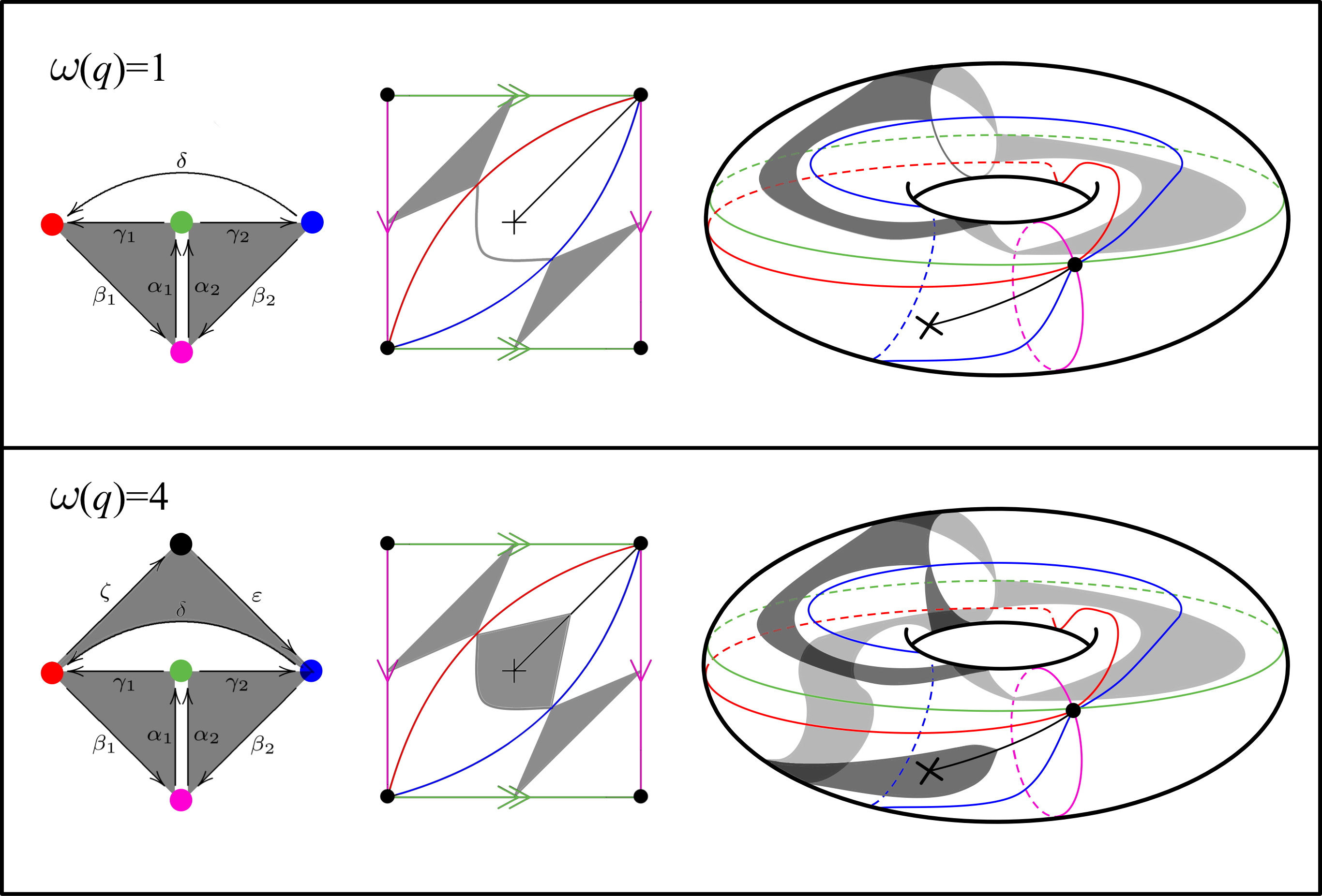
Figure 16. The geometric realization $Y(\tau,\omega)$ of the complex $C_{\bullet}(\tau,\omega)$ for the two possible values of $\omega$

Let $k$ be the pending arc in $\tau$, and let $\sigma$ be the triangulation of ${\mathbf{\Sigma}}$ obtained from $\tau$ by flipping $k$.

Example 9.4.

Suppose $\omega(q)=1$. Then the bijective function $Z^{1}(\tau,\omega)\rightarrow Z^{1}(\sigma,\omega)$ that underlies the definition of colored flip is not $\mathbb{F}_{2}$-linear. However, it does have the property of being constant on any given cohomology class, hence it induces a (non-linear) bijective function $H^{1}(\tau,\omega)\rightarrow H^{1}(\sigma,\omega)$.

The set $Q^{\prime}_{1}(\tau,\omega)=\{\alpha_{1},\beta_{1},\gamma_{1},\alpha_{2},\beta_{2},\gamma_{2},\delta\}$ is an $\mathbb{F}_{2}$-basis of $C_{1}(\tau,\omega)$, and a function $\xi\in\operatorname{Hom}_{\mathbb{F}_{2}}(C_{1}(\tau,\omega),\mathbb{F}_{2})$ is a 1-cocycle of the cochain complex $C^{\bullet}(\tau,\omega)$ if and only if

$$\xi(\alpha_{1})+\xi(\beta_{1})+\xi(\gamma_{1})=0=\xi(\alpha_{2})+\xi(\beta_{2})+\xi(\gamma_{2}).$$

Furthermore, if $\{\alpha_{1}^{\vee},\beta_{1}^{\vee},\gamma_{1}^{\vee},\alpha_{2}^{\vee},\beta_{2}^{\vee},\gamma_{2}^{\vee},\delta^{\vee}\}$ is the basis of $C^{1}(\tau,\omega)$ which is $\mathbb{F}_{2}$-dual to $Q^{\prime}_{1}(\tau,\omega)$, then the cohomology classes of the cocycles

$$\alpha_{1}^{\vee}+\beta_{1}^{\vee}\ \ \ \text{and}\ \ \ \delta^{\vee}$$

form an $\mathbb{F}_{2}$-basis of $H^{1}(C^{\bullet}(\tau,\omega))$. Therefore,

$$H^{1}(C^{\bullet}(\tau,\omega))=\{[0],[\alpha_{1}^{\vee}+\beta_{1}^{\vee}],[\delta^{\vee}],[\alpha_{1}^{\vee}+\beta_{1}^{\vee}+\delta^{\vee}]\}$$

and hence, the connected components of the flip graph $\mathcal{H}({\mathbf{\Sigma}_{\omega}})$ are precisely the connected components where the vertices $(\tau,[0])$, $(\tau,[\alpha_{1}^{\vee}+\beta_{1}^{\vee}])$, $(\tau,[\delta^{\vee}])$ and $(\tau,[\alpha_{1}^{\vee}+\beta_{1}^{\vee}+\delta^{\vee}])$ lie.

Let us abuse notation and use the same greek letters from Figure 15 to denote the names of the arrows of $Q(\sigma,\omega)$. Then the aforementioned bijective function $Z^{1}(\tau,\omega)\rightarrow Z^{1}(\sigma,\omega)$ is given by the rule

$$\xi\mapsto\xi+\delta^{\vee},$$

and the induced function $H^{1}(\tau,\omega)\rightarrow H^{1}(\sigma,\omega)$ is given by

$[0]\mapsto[\delta^{\vee}]$,	$[\alpha_{1}^{\vee}+\beta_{1}^{\vee}]\mapsto[\alpha_{1}^{\vee}+\beta_{1}^{\vee}+\delta^{\vee}]$,
$[\delta^{\vee}]\mapsto[0]$,	$[\alpha_{1}^{\vee}+\beta_{1}^{\vee}+\delta^{\vee}]\mapsto[\alpha_{1}^{\vee}+\beta_{1}^{\vee}]$.

Example 9.5.

Suppose $\omega(q)=4$. Then the bijective function $Z^{1}(\tau,\omega)\rightarrow Z^{1}(\sigma,\omega)$ that underlies the definition of colored flip is $\mathbb{F}_{2}$-linear and constant on any given cohomology class, hence it induces a (linear) bijective function $H^{1}(\tau,\omega)\rightarrow H^{1}(\sigma,\omega)$.

The set $Q^{\prime}_{1}(\tau,\omega)=\{\alpha_{1},\beta_{1},\gamma_{1},\alpha_{2},\beta_{2},\gamma_{2},\delta,\varepsilon,\zeta\}$ is an $\mathbb{F}_{2}$-basis of $C_{1}(\tau,\omega)$, and a function $\xi\in\operatorname{Hom}_{\mathbb{F}_{2}}(C_{1}(\tau,\omega),\mathbb{F}_{2})$ is a 1-cocycle of the cochain complex $C^{\bullet}(\tau,\omega)$ if and only if

$$\xi(\alpha_{1})+\xi(\beta_{1})+\xi(\gamma_{1})=\xi(\alpha_{2})+\xi(\beta_{2})+\xi(\gamma_{2})=\xi(\delta)+\xi(\varepsilon)+\xi(\zeta)=0.$$

Furthermore, if $\{\alpha_{1}^{\vee},\beta_{1}^{\vee},\gamma_{1}^{\vee},\alpha_{2}^{\vee},\beta_{2}^{\vee},\gamma_{2}^{\vee},\delta^{\vee},\varepsilon^{\vee},\zeta^{\vee}\}$ is the basis of $C^{1}(\tau,\omega)$ which is $\mathbb{F}_{2}$-dual to $Q^{\prime}_{1}(\tau,\omega)$, then the cohomology classes of the cocycles

$$\alpha_{1}^{\vee}+\beta_{1}^{\vee}\ \ \ \text{and}\ \ \ \delta^{\vee}+\varepsilon^{\vee}$$

form an $\mathbb{F}_{2}$-basis of $H^{1}(C^{\bullet}(\tau,\omega))$. Therefore,

$$H^{1}(C^{\bullet}(\tau,\omega))=\{[0],[\alpha_{1}^{\vee}+\beta_{1}^{\vee}],[\delta^{\vee}+\varepsilon^{\vee}],[\alpha_{1}^{\vee}+\beta_{1}^{\vee}+\delta^{\vee}+\varepsilon^{\vee}]\}$$

and hence, the connected components of the flip graph $\mathcal{H}({\mathbf{\Sigma}_{\omega}})$ are precisely the connected components where the vertices $(\tau,[0])$, $(\tau,[\alpha_{1}^{\vee}+\beta_{1}^{\vee}])$, $(\tau,[\delta^{\vee}+\varepsilon^{\vee}])$ and $(\tau,[\alpha_{1}^{\vee}+\beta_{1}^{\vee}+\delta^{\vee}+\varepsilon^{\vee}])$ lie.

Let us abuse notation and use the same greek letters from Figure 15 to denote the names of the arrows of $Q(\sigma,\omega)$. Then, using the fact that $+=-$ in every $\mathbb{F}_{2}$-vector space, the aforementioned functions $Z^{1}(\tau,\omega)\rightarrow Z^{1}(\sigma,\omega)$ and $H^{1}(\tau,\omega)\rightarrow H^{1}(\sigma,\omega)$ are the identity.

In both Examples 9.4 and 9.5, a bit of work shows that for every cocycle $\xi\in Z^{1}(\tau,\omega)$ the Jacobian algebra $\mathcal{P}(A(\tau,\xi),S(\tau,\xi))$ is infinite-dimensional over $F$. Indeed, for any of the two values of $\omega$ and any cocycle $\xi\in Z^{1}(\tau,\omega)$ we have $S(\tau,\xi)=\alpha_{1}\beta_{1}\gamma_{1}+\alpha_{2}\beta_{2}\gamma_{2}+\delta\varepsilon\zeta\in R\langle\langle A(\tau,\xi)\rangle\rangle$, from which it follows that no positive power of $\alpha_{1}\beta_{2}\varepsilon\zeta\gamma_{1}\alpha_{2}\beta_{1}\delta\gamma_{2}$ belongs to the Jacobian ideal $J(S(\tau,\xi))\subseteq R\langle\langle A(\tau,\xi)\rangle\rangle$.

10. Cohomology and Jacobian algebras

Let ${\mathbf{\Sigma}_{\omega}}=(\Sigma,\mathbb{M},\mathbb{O},\omega)$ be either unpunctured with (arbitrarily many) weighted orbifold points, or once-punctured closed with (arbitrarily many) weighted orbifold points, see Definition 2.5 and the paragraphs of Section 2 that precede Remark 2.1. Let $\tau$ be a triangulation of ${\mathbf{\Sigma}}=(\Sigma,\mathbb{M},\mathbb{O})$, and $E/F$ be a field extension as in Section 6.1. For each 1-cocycle $\xi\in{Z^{1}({\tau,\omega})}\subseteq C^{1}(\tau,\omega)=\operatorname{Hom}_{\mathbb{F}_{2}}(\mathbb{F}_{2}X_{1}({\tau,\omega}),\mathbb{F}_{2})$, we have associated to the colored triangulation $(\tau,\xi)$ a species $A(\tau,\xi)$ over $E/F$ and a potential $S(\tau,\xi)\in R\langle\langle A(\tau,\xi)\rangle\rangle$. Recall from [27, Definition 3.11] that for each arrow $a$ of $A(\tau,\xi)$ the cyclic derivative with respect to $a$ is defined to be

(10.1) $$\partial_{a}(\omega_{0}a_{1}\omega_{1}a_{2}\omega_{2}\ldots\omega_{\ell-1}a_{\ell}\omega_{\ell})=\sum_{j=1}^{\ell}\delta_{a,a_{j}}\pi_{g(\tau,\xi)_{a}^{-1}}(\omega_{j}a_{j+1}\ldots a_{\ell}\omega_{\ell}\omega_{0}a_{1}\ldots a_{j-1}\omega_{j-1})$$

for each cyclic path $\omega_{0}a_{1}\omega_{1}a_{2}\omega_{2}\ldots\omega_{\ell-1}a_{\ell}\omega_{\ell}\in R\langle\langle A(\tau,\xi)\rangle\rangle$, where $\delta_{a,a_{k}}$ is the Kronecker delta between $a$ and $a_{k}$, and $\pi_{g(\tau,\xi)_{a}^{-1}}(x)=\frac{1}{d_{h(a),t(a)}}\sum_{\nu\in\mathcal{B}_{h(a),t(a)}}g(\tau,\xi)_{a}^{-1}(\nu^{-1})x\nu$. Recall also that the Jacobian ideal $J(S(\tau,\xi))$ is the topological closure of the two-sided ideal of $R\langle\langle A(\tau,\xi)\rangle\rangle$ generated by $\{\partial_{a}(S(\tau,\xi))\ |\ a$ is an arrow of $Q(\tau,\omega)\}$, and that the Jacobian algebra of $(A(\tau,\xi),S(\tau,\xi))$ is the quotient $\mathcal{P}((A(\tau,\xi),S(\tau,\xi))):=R\langle\langle A(\tau,\xi)\rangle\rangle/J(S(\tau,\xi))$. The main result of this section is the following:

Theorem 10.1.

Let $\xi_{1},\xi_{2}\in Z^{1}(\tau,\omega)$ be 1-cocycles of the cochain complex ${C^{\bullet}({\tau,\omega})}$. If $(\Sigma,\mathbb{M},\mathbb{O})$ is unpunctured, then the following two statements are equivalent:

• $[\xi_{1}]=[\xi_{2}]$ in the first cohomology group $H^{1}(C^{\bullet}(\tau,\omega))$;

• the Jacobian algebras $\mathcal{P}((A(\tau,\xi_{1}),S(\tau,\xi_{1})))$ and $\mathcal{P}((A(\tau,\xi_{2}),S(\tau,\xi_{2})))$ are isomorphic through an $F$-linear ring isomorphism acting as the identity on $\{e_{k}\ |\ k\in Q_{0}\}$.

If $(\Sigma,\mathbb{M},\mathbb{O})$ is once-punctured closed, then the first statement implies the second one.

Proof.

Suppose that $\xi_{1}$ and $\xi_{2}$ are homologous 1-cocycles of the cochain complex ${C^{\bullet}({\tau,\omega})}$. This means that there exists a function $\phi:Q^{\prime}_{0}({\tau,\omega})\rightarrow\mathbb{F}_{2}$ such that

(10.2) $$\xi_{2}(a)-\xi_{1}(a)=\phi(h(a))-\phi(t(a)) a\in X_{1}({\tau,\omega})=Q^{\prime}_{1}({\tau,\omega})$$ for every .

We shall use $\phi$ to produce a ring automorphism $\Psi^{(0)}:R\rightarrow R$ and a group isomorphism $\Psi^{(1)}:A(\tau,\xi_{1})\rightarrow A(\tau,\xi_{2})$ such that $\Psi^{(1)}(ra)=\Psi^{(0)}(r)\Psi^{(1)}(a)$ and $\Psi^{(1)}(ar)=\Psi^{(1)}(a)\Psi^{(0)}(r)$ for all $r\in R$ and all $a\in A(\tau,\xi_{1})$.

For each $j\in\tau$ such that $d({\tau,\omega})_{j}=4$ choose an element $\lambda_{j}\in G_{k}=\operatorname{Gal}(E/F)$ such that $\lambda_{j}|_{L}=\theta^{\phi(j)}$. For $k\in\tau$, we set

$$\psi_{k}=\begin{cases}11_{F}&\text{if $d({\tau,\omega})_{k}=1$;}\\ \theta^{\phi(k)}&\text{if $d({\tau,\omega})_{k}=2$;}\\ \lambda_{k}&\text{if $d({\tau,\omega})_{k}=4$.}\end{cases}$$

Then we define $\Psi^{(0)}\left(\sum_{k\in\tau}x_{k}e_{k}\right)=\sum_{k\in\tau}\psi_{k}(x_{k})e_{k}$. It is clear that $\Psi^{(0)}$ is a ring automorphism of $R$.

Now, let $a$ be an arrow of the quiver $Q({\tau,\omega})$. If $d({\tau,\omega})_{h(a)}d({\tau,\omega})_{t(a)}\neq 16$, then from (10.2) we can easily deduce that in the bimodule $F_{h(a)}^{g(\tau,\xi_{2})_{a}}\otimes_{F_{h(a),t(a)}}F_{t(a)}$ we have

$$\psi_{h(a)}(x)\otimes\psi_{t(a)}(zy) = \psi_{h(a)}(x)\otimes\psi_{t(a)}(z)\psi_{t(a)}(y)$$

$$= \psi_{h(a)}(x)g(\tau,\xi_{2})_{a}(\psi_{t(a)}(z))\otimes\psi_{t(a)}(y)$$

$$= \psi_{h(a)}(x)\psi_{h(a)}(g(\tau,\xi_{1})_{a}(z))\otimes\psi_{t(a)}(y)$$

for $x\in F_{h(a)}$, $y\in F_{t(a)}$ and $z\in F_{h(a),t(a)}$, and hence, that the rule $x\otimes y\mapsto\psi_{h(a)}(x)\otimes\psi_{t(a)}(y)$ produces a well-defined group homomorphism $F_{h(a)}^{g(\tau,\xi_{1})_{a}}\otimes_{F_{h(a),t(a)}}F_{t(a)}\rightarrow F_{h(a)}^{g(\tau,\xi_{2})_{a}}\otimes_{F_{h(a),t(a)}}F_{t(a)}$.

If, on the other hand, we have $d({\tau,\omega})_{h(a)}d({\tau,\omega})_{t(a)}=16$ instead, then $d({\tau,\omega})_{h(a)}=4=d({\tau,\omega})_{t(a)}$ and $Q({\tau,\omega})$ has exactly two arrows $\delta_{0}$ and $\delta_{1}$ going from $t(a)$ to $h(a)$ (of course, $a$ is one of these two arrows). From (10.2) and Definition 6.1 we deduce that $g(\tau,\xi_{2})_{\delta_{0}}|_{L}=g(\tau,\xi_{2})_{\delta_{1}}|_{L}=(\psi_{h(a)}g(\tau,\xi_{1})_{\delta_{0}}\psi_{t(a)}^{-1})|_{L}=(\psi_{h(a)}g(\tau,\xi_{1})_{\delta_{1}}\psi_{t(a)}^{-1})|_{L}$, and consequently, that $\{g(\tau,\xi_{2})_{\delta_{0}},g(\tau,\xi_{2})_{\delta_{1}}\}=\{\psi_{h(a)}g(\tau,\xi_{1})_{\delta_{0}}\psi_{t(a)}^{-1},\psi_{h(a)}g(\tau,\xi_{1})_{\delta_{1}}\psi_{t(a)}^{-1}\}$. Hence, there is a permutation $p:\{\delta_{0},\delta_{1}\}\rightarrow\{\delta_{0},\delta_{1}\}$ such that $g(\tau,\xi_{2})_{p(\delta_{i})}=\psi_{h(a)}g(\tau,\xi_{1})_{\delta_{i}}\psi_{t(a)}^{-1}$ for $i\in\{0,1\}$. Therefore, there is a well-defined group homomorphism $F_{h(a)}^{g(\tau,\xi_{1})_{a}}\otimes_{F_{h(a),t(a)}}F_{t(a)}\rightarrow F_{h(a)}^{g(\tau,\xi_{2})_{p(a)}}\otimes_{F_{h(a),t(a)}}F_{t(a)}$ given by the rule $x\otimes y\mapsto\psi_{h(a)}(x)\otimes\psi_{t(a)}(y)$.

We have thus constructed a group homomorphism for each arrow of the quiver $Q({\tau,\omega})$. Assembling all the group homomorphisms constructed, and recalling that $A(\tau,\xi_{j})=\bigoplus_{a\in Q_{1}(\tau,\omega)}F_{h(a)}^{g(\tau,\xi_{j})_{a}}\otimes_{F_{h(a),t(a)}}F_{t(a)}$ for $j\in\{1,2\}$, we obtain a group homomorphism $\Psi^{(1)}:A(\tau,\xi_{1})\rightarrow A(\tau,\xi_{2})$. It is clear that $\Psi^{(1)}$ is a group isomorphism and that it satisfies $\Psi^{(1)}(ra)=\Psi^{(0)}(r)\Psi^{(1)}(a)$ and $\Psi^{(1)}(ar)=\Psi^{(1)}(a)\Psi^{(0)}(r)$ for all $r\in R$ and all $a\in A(\tau,\xi_{1})$. A minor variation of [27, Proposition 2.11] then implies that there exists a continuous ring isomorphism $\Psi:R\langle\langle A(\tau,\xi_{1})\rangle\rangle\rightarrow R\langle\langle A(\tau,\xi_{2})\rangle\rangle$ such that $\Psi|_{R}=\Psi^{(0)}$ and $\Psi|_{A(\tau,\xi_{1})}=\Psi^{(1)}$. Since $\Psi^{(0)}$ is clearly $F$-linear, $\Psi$ is $F$-linear.

Consider the potential $\Psi(S(\tau,\xi_{1}))=\sum_{\triangle}\Psi(S^{\triangle}(\tau,\xi_{1}))$ (which may be not equal to $S(\tau,\xi_{2})$ because of the presence of the factor $u$ in the first item of Definition 6.9). Using the fact that $u$ is an eigenvector of the two elements of $\operatorname{Gal}(L/F)$ with the corresponding eigenvalues lying in $F$ (in fact, these eigenvalues are $1$ and $-1$), it is fairly easy to check that $\Psi(\partial_{a}(S(\tau,\xi_{1})))=\partial_{\Psi(a)}(\Psi(S(\tau,\xi_{1})))$ for every arrow $a$ of the quiver $Q({\tau,\omega})$. It follows that $\Psi(J(S(\tau,\xi_{1})))\subseteq J(\Psi(S(\tau,\xi_{1})))$. Applying the same reasoning to $\Psi^{-1}$ we obtain $\Psi^{-1}(J(\Psi(S(\tau,\xi_{1}))))\subseteq J(\Psi^{-1}\Psi(S(\tau,\xi_{1})))=J(S(\tau,\xi_{1}))$, and hence $J(\Psi(S(\tau,\xi_{1})))=\Psi\Psi^{-1}(J(\Psi(S(\tau,\xi_{1}))))\subseteq\Psi(J(S(\tau,\xi_{1})))$. Therefore, $\Psi(J(S(\tau,\xi_{1})))=J(\Psi(S(\tau,\xi_{1})))$.

Finally, using again the fact that $u$ is an eigenvector of the two elements of $\operatorname{Gal}(L/F)$ with the corresponding eigenvalues lying in $F$, we see that the relation that $\Psi(S(\tau,\xi_{1}))$ keeps with $S(\tau,\xi_{2})$ is that it can be obtained from it by multiplying some of its constituent cyclic paths by elements of $F$ (actually, these elements are $1$ and $-1$). And noticing that $S(\tau,\xi_{2})$ has an expression as an $F$-linear combination of cyclic paths that has the property that every cyclic path appearing in it involves at least one arrow that does not appear in any other cyclic path in the expression, it is easy to produce an $R$-algebra automorphism $\Phi$ of $R\langle\langle A(\tau,\xi_{2})\rangle\rangle$ that sends $\Psi(S(\tau,\xi_{1}))$ to a potential cyclically equivalent to $S(\tau,\xi_{2})$. By the previous paragraph and [27, Lemma 10.3 and the paragraph that precedes it], we deduce that $\Phi\Psi(J(S(\tau,\xi_{1})))=\Phi(J(\Psi(S(\tau,\xi_{1}))))=J(\Phi\Psi(S(\tau,\xi_{1})))=J(S(\tau,\xi_{2}))$.

We have thus proved that, regardless of whether ${\mathbf{\Sigma}}$ is unpunctured or once-punctured closed, if $[\xi_{1}]=[\xi_{2}]$ in $H^{1}(C^{\bullet}(\tau,\omega))$, then the Jacobian algebras $\mathcal{P}((A(\tau,\xi_{1}),S(\tau,\xi_{1})))$ and $\mathcal{P}((A(\tau,\xi_{2}),S(\tau,\xi_{2})))$ are isomorphic through an $F$-linear ring isomorphism acting as the identity on $\{e_{k}\ |\ k\in Q_{0}\}$. The converse implication for unpunctured surfaces requires some preparation.

From this point to the end of this section we shall suppose that ${\mathbf{\Sigma}}$ is unpunctured with non-empty boundary. We start by establishing a result of independent interest, namely:

Theorem 10.2.

If ${\mathbf{\Sigma}_{\omega}}=(\Sigma,\mathbb{M},\mathbb{O},\omega)$ is an unpunctured surface with weighted orbifold points, then for any colored triangulation $(\tau,\xi)$ of ${\mathbf{\Sigma}_{\omega}}$ the Jacobian algebra $\mathcal{P}(A(\tau,\xi),S(\tau,\xi))$ has finite dimension over $F$; more precisely, there exists a positive integer $t$ such that $\mathfrak{m}^{t}\subseteq J(S(\tau,\xi))\subseteq\mathfrak{m}^{2}$, where $\mathfrak{m}$ is the two-sided ideal of $R\langle\langle A(\tau,\xi)\rangle\rangle$ generated by the arrows of the underlying quiver $Q(\tau,\omega)$.

Proof.

Let ${\mathbf{\Sigma}_{\omega}}$ be as in the hypothesis of the theorem, and let $(\tau,\xi)$ be any colored triangulation of ${\mathbf{\Sigma}_{\omega}}$. For every arrow $a$ of $Q(\tau,\omega)$, the explicit expression of $\partial_{a}(S(\tau,\xi))$ as an element of $R\langle\langle A(\tau,\xi)\rangle\rangle$ is given by the table depicted in Figure 17. Hence, for any two arrows $b$ and $c$ of $Q(\tau,\omega)$ that are induced by the same triangle, if $t(b)=h(c)$ and $t(b)$ is not a pending arc, then $bzc\in J(S(\tau,\xi))$ for every element $z\in F_{t(b)}e_{t(b)}=Le_{t(b)}\subseteq R$.

	$\partial_{\alpha}(S(\tau,\xi))$	$\partial_{\beta}(S(\tau,\xi))$	$\partial_{\gamma}(S(\tau,\xi))$	$\partial_{\delta_{0}}(S(\tau,\xi))$	$\partial_{\delta_{1}}(S(\tau,\xi))$
	$\beta\gamma$	$\gamma\alpha$	$\alpha\beta$
	$\begin{array}[]{l}\frac{1}{2}(\beta\gamma+\\[-3.0pt] \theta^{-\xi(\alpha)}(u^{-1})\beta\gamma u)\end{array}$	$\gamma\alpha$	$\alpha\beta$
	$\beta\gamma$	$\gamma\alpha$	$\alpha\beta$
		$\gamma\delta_{0}+u\gamma\delta_{1}$	$\delta_{0}\beta+\delta_{1}\beta u$	$\beta\gamma$	$\beta u\gamma$
	$\beta\gamma$	$\gamma\alpha$	$\begin{array}[]{l}\frac{1}{2}(\alpha\beta+\\[-3.0pt] \theta^{-\xi(\gamma)}(u^{-1})\alpha\beta u)\end{array}$
	$\beta\gamma$	$\begin{array}[]{l}\frac{1}{2}(\gamma\alpha+\\[-3.0pt] \theta^{-\xi(\beta)}(u^{-1})\gamma\alpha u)\end{array}$	$\alpha\beta$
		$\gamma(\delta_{0}+\delta_{1})$	$(\delta_{0}+\delta_{1})\beta$	$\begin{array}[]{l}\frac{1}{2}(\beta\gamma+\\[-3.0pt] \rho^{-\ell}(v^{-1})\beta\gamma v)\end{array}$	$\begin{array}[]{l}\frac{1}{2}(\beta\gamma+\\[-3.0pt] \rho^{-\ell-2}(v^{-1})\beta\gamma v)\end{array}$

Figure 17.

For each marked point $m\in\mathbb{M}$, let $t_{m}$ be the number of arcs in $\tau$ that are incident to $m$, counted with multiplicity (so that loops based at $m$ contribute twice to $t_{m}$), and let $t=\max\{t_{m}\ |\ m\in\mathbb{M}\}$. Then the previous paragraph and the fact that the boundary of $\Sigma$ is not empty imply that any element of $R\langle\langle A(\tau,\xi)\rangle\rangle$ which happens to be a path of length $t$ belongs to $J(S(\tau,\xi))$. The theorem follows. ∎

Definition 10.3.

We will say that an ideal $I$ of the complete path algebra $R\langle\langle A(\tau,\xi)\rangle\rangle$ is admissible, if there exists $t\in\mathbb{N}$ with $\mathfrak{m}^{t}\subseteq I\subseteq\mathfrak{m}^{2}$, where $\mathfrak{m}=\mathfrak{m}(A(\tau,\xi))$ is the (closed) ideal generated by $A(\tau,\xi)$.

The quotient $\Lambda=R\langle\langle A(\tau,\xi)\rangle\rangle/I$ by an admissible ideal $I$ is a finite-dimensional $F$-algebra with Jacobson radical $\mathrm{rad}(\Lambda)=\mathfrak{m}/I$. In particular, we can recover the $F$-algebra $R$ and the $R$-$R$-bimodule $A(\tau,\xi)$ from the $F$-algebra $\Lambda$ as $R\cong R\langle\langle A(\tau,\xi)\rangle\rangle/\mathfrak{m}\cong\Lambda/\mathrm{rad}(\Lambda)$ and $A(\tau,\xi)\cong\mathfrak{m}/\mathfrak{m}^{2}\cong\mathrm{rad}(\Lambda)/\mathrm{rad}^{2}(\Lambda)$.

Assume $\Lambda_{1}=R\langle\langle A(\tau,\xi_{1})\rangle\rangle/I_{1}$ and $\Lambda_{2}=R\langle\langle A(\tau,\xi_{2})\rangle\rangle/I_{2}$ for admissible ideals $I_{1}$ and $I_{2}$. For every $F$-algebra isomorphism $\Psi:\Lambda_{1}\to\Lambda_{2}$, we denote by $\Psi^{(0)}$ the $F$-algebra automorphism $R\cong\Lambda_{1}/\mathrm{rad}(\Lambda_{1})\to\Lambda_{2}/\mathrm{rad}(\Lambda_{2})\cong R$. Furthermore, for $R$-$R$-bimodules $M$ and $F$-algebra automorphisms $\psi:R\to R$, let $\psi_{*}M$ be the $R$-$R$-bimodule whose underlying $F$-vector space is $M$ with $R$-$R$-bimodule structure $rms:=\psi(r)\cdot_{M}m\cdot_{M}\psi(s)$ for $r,s\in R$ and $m\in\psi_{*}M$, where the symbol $\cdot_{M}$ is used for the left and right $R$-module action of the $R$-$R$-bimodule $M$.

Corollary 10.4.

If $\Psi:\mathcal{P}((A(\tau,\xi_{1}),S(\tau,\xi_{1})))\to\mathcal{P}((A(\tau,\xi_{2}),S(\tau,\xi_{2})))$ is an $F$-algebra isomorphism, then the $R$-$R$-bimodules $A(\tau,\xi_{1})$ and $\Psi^{(0)}_{*}A(\tau,\xi_{2})$ are isomorphic.

Proof.

Let $\mathfrak{r}_{1}$ and $\mathfrak{r}_{2}$ be the Jacobson radicals of $\mathcal{P}((A(\tau,\xi_{1}),S(\tau,\xi_{1})))$ and $\mathcal{P}((A(\tau,\xi_{2}),S(\tau,\xi_{2})))$, respectively. Given that $\Psi$ is an $F$-algebra isomorphism, it induces an isomorphism $\mathfrak{r}_{1}/\mathfrak{r}_{1}^{2}\to\Psi^{(0)}_{*}\big{(}\mathfrak{r}_{2}/\mathfrak{r}_{2}^{2}\big{)}$ of $R$-$R$-bimodules. This proves the corollary, since $\mathfrak{r}_{1}/\mathfrak{r}_{1}^{2}\cong A(\tau,\xi_{1})$ and $\mathfrak{r}_{2}/\mathfrak{r}_{2}^{2}\cong A(\tau,\xi_{2})$ since $J(S(\tau,\xi_{i}))$ is an admissible ideal of $R\langle\langle A(\tau,\xi_{i})\rangle\rangle$ for $i\in\{1,2\}$. ∎

Lemma 10.5.

Let $\psi:R\to R$ be an $F$-algebra automorphism with $\psi(e_{i})=e_{i}$ for all $i\in\tau$ such that the $R$-$R$-bimodules $A(\tau,\xi_{1})$ and $\psi_{*}A(\tau,\xi_{2})$ are isomorphic. Then, for all $i,j\in\tau$, the $F_{j}$-$F_{i}$-bimodules $e_{j}A(\tau,\xi_{1})e_{i}$ and $\psi_{*}(e_{j}A(\tau,\xi_{2})e_{i})$ are isomorphic.

Proof.

It is clear that $e_{j}A(\tau,\xi_{1})e_{i}\cong e_{j}(\psi_{*}(A(\tau,\xi_{2})))e_{i}=\psi_{*}(\psi(e_{j})A(\tau,\xi_{2})\psi(e_{i}))=\psi_{*}(e_{j}A(\tau,\xi_{2})e_{i})$. ∎

For $F$-algebra automorphisms $\psi:R\to R$ satisfying $\psi(e_{i})=e_{i}$ for all $i\in\tau$, denote by $\psi_{i}$ the automorphism $F_{i}\cong e_{i}Re_{i}\to e_{i}Re_{i}\cong F_{i}$ in $\operatorname{Gal}(F_{i}/F)$ induced by $\psi$.

Lemma 10.6.

Let $(\tau,\xi)$ be a colored triangulation and $\psi:R\to R$ an $F$-algebra automorphism satisfying $\psi(e_{i})=e_{i}$ for all $i\in\tau$. Then, for all $i,j\in\tau$, the $F_{j}$-$F_{i}$-bimodule $\psi_{*}(e_{j}A(\tau,\xi)e_{i})$ is isomorphic to $\bigoplus_{a}F_{j}^{\rho_{a}}\otimes_{F_{j,i}}F_{i}$, where $\rho_{a}:=\psi_{j}^{-1}g(\tau,\xi)_{a}\psi_{i}$ and the summation variable $a$ runs through all arrows in $Q_{1}(\tau,\omega)$ with $h(a)=j$ and $t(a)=i$.

Proof.

By definition $e_{j}A(\tau,\xi)e_{i}=\bigoplus_{a}F_{j}^{g(\tau,\xi)_{a}}\otimes_{F_{j,i}}F_{i}$. This implies the lemma, since each $\psi_{*}(F_{j}^{g(\tau,\xi)_{a}}\otimes_{F_{j,i}}F_{i})$ is a simple $F_{j}$-$F_{i}$-bimodule on which $F$ acts centrally and $\rho_{a}(r)x=xr$ for all $x\in\psi_{*}(F_{j}^{g(\tau,\xi)_{a}}\otimes_{F_{j,i}}F_{i})$ and $r\in F_{j,i}$. ∎

Corollary 10.7.

Let $(\tau,\xi_{1})$ and $(\tau,\xi_{2})$ be colored triangulations and $\psi:R\to R$ an $F$-algebra automorphism with $\psi(e_{i})=e_{i}$ for all $i\in\tau$ such that $A(\tau,\xi_{1})$ and $\psi_{*}A(\tau,\xi_{2})$ are isomorphic $R$-$R$-bimodules. Then there is a permutation $\pi$ of $Q_{1}(\tau,\omega)$ such that $h(\pi(a))=h(a)$, $t(\pi(a))=t(a)$, and $g(\tau,\xi_{1})_{a}=\psi_{h(a)}^{-1}g(\tau,\xi_{2})_{\pi(a)}\psi_{t(a)}$ for all $a\in Q_{1}(\tau,\omega)$.

Proof.

For all $i,j\in\tau$ we have $\bigoplus_{j\xleftarrow{a}i}F_{j}^{g(\tau,\xi_{1})_{a}}\otimes_{F_{j,i}}F_{i}=e_{j}A(\tau,\xi_{1})e_{i}\cong\psi_{*}(e_{j}A(\tau,\xi_{2})e_{i})\cong\bigoplus_{j\xleftarrow{a}i}F_{j}^{\rho_{a}}\otimes_{F_{j,i}}F_{i}$ with $\rho_{a}=\psi_{j}^{-1}g(\tau,\xi_{2})_{a}\psi_{i}$ by Lemmas 10.5 and 10.6. By the Krull-Schmidt theorem there is a permutation $\pi$ of $Q_{1}(\tau,\omega)$ such that, for all $a\in Q_{1}(\tau,\omega)$, it is $h(\pi(a))=h(a)$, $t(\pi(a))=t(a)$, and $F_{h(a)}^{g(\tau,\xi_{1})_{a}}\otimes_{F_{h(a),t(a)}}F_{t(a)}\cong F_{h(a)}^{\rho_{\pi(a)}}\otimes_{F_{h(a),t(a)}}F_{t(a)}$ as simple $F_{h(a)}$-$F_{t(a)}$-bimodules on which $F$ acts centrally. Hence, $g(\tau,\xi_{1})_{a}=\rho_{\pi(a)}=\psi_{h(a)}^{-1}g(\tau,\xi_{2})_{\pi(a)}\psi_{t(a)}$. ∎

Proposition 10.8.

Let $(\tau,\xi_{1})$ and $(\tau,\xi_{2})$ be colored triangulations, let $\psi:R\to R$ be an $F$-algebra automorphism satisfying $\psi(e_{i})=e_{i}$ for all $i\in\tau$, and let $\pi$ be a permutation of $Q_{1}(\tau,\omega)$ such that $h(\pi(a))=h(a)$, $t(\pi(a))=t(a)$, and $g(\tau,\xi_{1})_{a}=\psi_{h(a)}^{-1}g(\tau,\xi_{2})_{\pi(a)}\psi_{t(a)}$ for all $a\in Q_{1}(\tau,\omega)$. Then one has $[\xi_{1}]=[\xi_{2}]$ in ${H^{1}(C^{\bullet}({\tau,\omega}))}$.

Proof.

Recall from Subsection 6.1 that $\operatorname{Gal}(L/F)=\{11_{L},\theta\}$. Define a function $\phi:Q^{\prime}_{0}({\tau,\omega})\to\mathbb{F}_{2}$ by

$$\phi(k)\>:=\>\begin{cases}0&\text{if $\psi_{k}|_{L}=11_{L}$,}\\ 1&\text{if $\psi_{k}|_{L}=\theta$.}\end{cases}$$

For every $a\in Q^{\prime}_{1}({\tau,\omega})$, we can write $g(\tau,\xi_{1})_{a}|_{L}=\theta^{\xi_{1}(a)}$ and $g(\tau,\xi_{2})_{\pi(a)}|_{L}=\theta^{\xi_{2}(\pi(a))}$ according to Definition 6.1. Therefore $\theta^{\xi_{1}(a)}=g(\tau,\xi_{1})_{a}|_{L}=\psi_{h(a)}^{-1}|_{L}\cdot g(\tau,\xi_{2})_{\pi(a)}|_{L}\cdot\psi_{t(a)}|_{L}=\theta^{-\phi(h(a))}\cdot\theta^{\xi_{2}(\pi(a))}\cdot\theta^{\phi(t(a))}$. This can be rewritten as $\theta^{\xi_{2}(\pi(a))-\xi_{1}(a)}=\theta^{\phi(h(a))-\phi(t(a))}$ and is equivalent to

$$\xi_{2}(\pi(a))-\xi_{1}(a)\>=\>\phi(h(a))-\phi(t(a))\hskip 15.0pt\text{for every $a\in Q^{\prime}_{1}({\tau,\omega})$.}$$

For all $i,j\in\tau$, denote by $q_{j,i}$ the number of arrows from $i$ to $j$ in $Q^{\prime}_{1}({\tau,\omega})$. We already may conclude that

$$\xi_{2}(a)-\xi_{1}(a)\>=\>\phi(h(a))-\phi(t(a))\hskip 15.0pt\text{for every $a\in Q^{\prime}_{1}({\tau,\omega})$ with $q_{h(a),t(a)}=1$.}$$

Observe that, for all $a\in Q^{\prime}_{1}({\tau,\omega})$, it is $q_{h(a),t(a)}\leq 2$. Moreover, $q_{h(a),t(a)}=1$, if $d(\tau,\omega)_{h(a)}=4$ or $d(\tau,\omega)_{t(a)}=4$. For every arrow $a\in Q^{\prime}_{1}({\tau,\omega})$ with $q_{h(a),t(a)}\neq 1$, we therefore have $d(\tau,\omega)_{h(a)}=2=d(\tau,\omega)_{t(a)}$ and $q_{h(a),t(a)}=2$. From now on, let us assume that $a$ is such an arrow.

If $a$ is induced by an interior triangle $\triangle$ of $\tau$, then necessarily $\triangle\in X_{2}({\tau,\omega})$. In this case, let $b,c\in Q^{\prime}_{1}({\tau,\omega})$ be the other two arrows induced by $\triangle$ with $t(b)=h(c)$, $t(c)=h(a)$, and $t(a)=h(b)$. By inspecting the puzzle-piece decomposition of $\tau$, it is not hard to see that $q_{h(b),t(b)}=1=q_{h(c),t(c)}$. Consequently, $\xi_{2}(b)-\xi_{1}(b)=\phi(h(b))-\phi(t(b))$ and $\xi_{2}(c)-\xi_{1}(c)=\phi(h(c))-\phi(t(c))$. In addition, since $\xi_{1}$ and $\xi_{2}$ are $1$-cocycles, we also have $\xi_{1}(a)+\xi_{1}(b)+\xi_{1}(c)=0$ and $\xi_{2}(a)+\xi_{2}(b)+\xi_{2}(c)=0$. Combining all this yields

$$\begin{array}[]{lclcl}\xi_{2}(a)-\xi_{1}(a)&=&-(\xi_{2}(b)+\xi_{2}(c))+(\xi_{1}(b)+\xi_{1}(c))\\ &=&-(\xi_{2}(b)-\xi_{1}(b))-(\xi_{2}(c)-\xi_{1}(c))\\ &=&-(\phi(h(b))-\phi(t(b)))-(\phi(h(c))-\phi(t(c)))\\ &=&-(\phi(t(a))-\phi(h(c)))-(\phi(h(c))-\phi(h(a)))&=&\phi(h(a))-\phi(t(a))\,.\end{array}$$

If $a$ is not induced by an interior triangle of $\tau$, but the parallel arrow $\pi(a)$ is induced by an interior triangle of $\tau$, the argument just given (with $a$ replaced by $\pi(a)$) shows that $\xi_{2}(\pi(a))-\xi_{1}(\pi(a))=\phi(h(a))-\phi(t(a))$. On the other hand, we already know that $\xi_{2}(a)-\xi_{1}(\pi(a))=\phi(h(a))-\phi(t(a))$, since $\pi(\pi(a))=a$. Hence, $\xi_{2}(\pi(a))=\xi_{2}(a)$.

Let us finally consider the case where neither $a$ nor $\pi(a)$ is induced by an interior triangle of $\tau$. Then $a$ and $\pi(a)$ are each induced by a triangle with a boundary segment as one of its sides. Moreover, the two triangles inducing $a$ and $\pi(a)$ share the two sides $h(a)$ and $t(a)$. It is easy to see (from the puzzle-piece decomposition of $\tau$) that ${\mathbf{\Sigma}}$ is a cylinder with two marked points and without orbifold points. In particular, the quiver $Q^{\prime}({\tau,\omega})$ consists just of the two parallel arrows $a$ and $\pi(a)$. Define $\phi^{\prime}:Q^{\prime}_{0}({\tau,\omega})\to\mathbb{F}_{2}$ by $\phi^{\prime}(h(a)):=\xi_{2}(a)$ and $\phi^{\prime}(t(a)):=\xi_{1}(a)$. Then, obviously, $\xi_{2}(a)-\xi_{1}(a)=\phi^{\prime}(h(a))-\phi^{\prime}(t(a))$. Furthermore, using $\xi_{2}(\pi(a))-\xi_{1}(a)=\phi(h(a))-\phi(t(a))=\xi_{2}(a)-\xi_{1}(\pi(a))$,

$$\begin{array}[]{lclclcl}\xi_{2}(\pi(a))-\xi_{1}(\pi(a))&=&(\xi_{2}(\pi(a))-\xi_{2}(a))+(\xi_{2}(a)-\xi_{1}(\pi(a))\\ &=&(\xi_{2}(\pi(a))-\xi_{2}(a))+(\xi_{2}(\pi(a))-\xi_{1}(a))&=&\xi_{2}(a)-\xi_{1}(a)&=&\phi^{\prime}(h(a))-\phi^{\prime}(t(a))\,.\end{array}$$

So, if ${\mathbf{\Sigma}}$ is a cylinder with two marked points and without orbifold points, we get $[\xi_{1}]=[\xi_{2}]$ in cohomology, since the $\mathbb{F}_{2}$-linear extension $\widehat{\phi}^{\prime}$ of $\phi^{\prime}$ defines a coboundary $\xi_{2}-\xi_{1}=\widehat{\phi}^{\prime}\circ\partial_{1}$.

For the general situation, but excluding the case in which ${\mathbf{\Sigma}}$ is a cylinder with two marked points and without orbifold points, we have seen before that $\xi_{2}(a)-\xi_{1}(a)=\phi(h(a))-\phi(t(a))$ for all $a\in Q^{\prime}_{1}({\tau,\omega})$. Again, this readily implies the identity $[\xi_{1}]=[\xi_{2}]$ in cohomology. ∎

To finish the proof of Theorem 10.1, suppose that $\Psi:\mathcal{P}((A(\tau,\xi_{1}),S(\tau,\xi_{1})))\to\mathcal{P}((A(\tau,\xi_{2}),S(\tau,\xi_{2})))$ is an $F$-linear ring isomorphism satisfying $\Psi(e_{k})=e_{k}$ for all $k\in\tau$. Let us abbreviate $\Psi^{(0)}$ as $\psi$. Corollary 10.4 shows that $A(\tau,\xi_{1})$ and $\psi_{*}A(\tau,\xi_{2})$ are isomorphic $R$-$R$-bimodules. According to Corollary 10.7 there exists a permutation $\pi$ of $Q_{1}(\tau,\omega)$ such that $h(\pi(a))=h(a)$, $t(\pi(a))=t(a)$, and $g(\tau,\xi_{1})_{a}=\psi_{h(a)}^{-1}g(\tau,\xi_{2})_{\pi(a)}\psi_{t(a)}$ for all $a\in Q_{1}(\tau,\omega)$. Now Proposition 10.8 yields $[\xi_{1}]=[\xi_{2}]$.

Theorem 10.1 is proved. ∎

11. Classification of non-degenerate SPs

The goal of this section is to show that for unpunctured surfaces the SPs $(A(\tau,\xi),S(\tau,\xi))$ defined in Section 6 are unique in the sense that if the pair $(\tau,\omega)$ and the ground degree-$d$ cyclic Galois extension $E/F$ are fixed, and if we are given a non-degenerate SP $(A,W)$ such that $A$ is a species realization over $E/F$ of the skew-symmetrizable matrix $B(\tau,\omega)$, then $(A,W)$ is right-equivalent to $(A(\tau,\xi),S(\tau,\xi))$ for some 1-cocycle $\xi\in Z^{1}(\tau,\omega)\subseteq C^{1}(\tau,\omega)$ (see Theorem 11.8 below, compare to [25, Theorems 8.4 and 8.21]).

The following lemma is the very reason why in this paper we have restricted our attention to the species that arise from 1-cocycles of the cochain complexes $C^{\bullet}(\tau,\omega)$. Roughly speaking, it says that certain “cocycle condition” is necessarily satisfied by some 3-vertex species if they are to admit non-degenerate potentials.

Lemma 11.1.

Let $(Q,\mathbf{d})$ be any of the three weighted quivers depicted in Figure 18, $d$ the least common multiple of the integers conforming the tuple $\mathbf{d}$, $E/F$ a degree-$d$ cyclic Galois field extension such that $F$ contains a primitive $d^{\operatorname{th}}$ root of unity, $g:Q_{1}\rightarrow\bigcup_{i,j\in Q_{0}}\operatorname{Gal}(F_{i,j}/F)$ a modulating function for $(Q,\mathbf{d})$ over $E/F$, and $A$ the species of the triple $(Q,\mathbf{d},g)$.

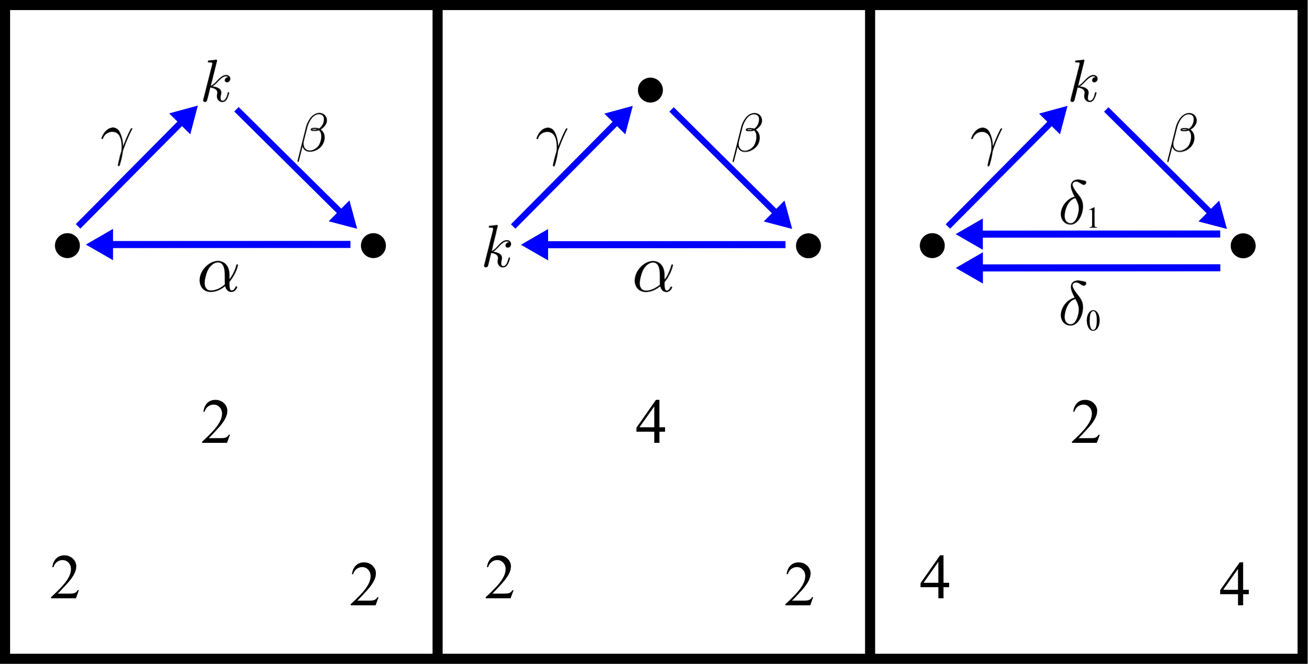
Figure 18.

If $A$ admits a non-degenerate potential, then the following identities hold in the Galois group $\operatorname{Gal}(L/F)\cong\mathbb{Z}/2\mathbb{Z}$:

(11.1) $$g_{\beta}g_{\gamma}=\begin{cases}g_{\alpha}^{-1}&\text{if $(Q,\mathbf{d})$ is the weighted quiver}\\ &\text{on the left or in the middle of Figure \ref{Fig:3_critical_quivers};}\\ g_{\delta_{0}}^{-1}|_{L}=g_{\delta_{1}}^{-1}|_{L}&\text{if $(Q,\mathbf{d})$ is the weighted quiver}\\ &\text{on the farthest right of Figure \ref{Fig:3_critical_quivers}}.\end{cases}$$

If $(Q,\mathbf{d})$ is the weighted quiver on the farthest right of Figure 18, then in the Galois group $\operatorname{Gal}(E/F)\cong\mathbb{Z}/4\mathbb{Z}$ we have $g_{\delta_{0}}\neq g_{\delta_{1}}$.

Proof.

In virtue of [27, Definitions 3.19 and 3.22], Lemma 11.1 is a direct consequence of [27, Example 3.12]. We shall elaborate only for the sake of clarity. Assume that $W\in R\langle\langle A\rangle\rangle$ is a potential such that $(A,W)$ is a non-degenerate SP.

Case 1.

Suppose that $(Q,\mathbf{d})$ is the weighted quiver on the farthest left of Figure 18. Up to cyclical equivalence, we can assume that $W=\sum_{n\geq 1}x_{n}(\alpha\beta\gamma)^{n}$ for some elements $x_{n}\in E$. By [27, Definition 3.19-(3)], in the complete path algebra of the species $\widetilde{\mu}_{k}(A)$ we have

$$\widetilde{\mu}_{k}(W)=\left(\sum_{n\geq 1}x_{n}(\alpha[\beta\gamma]_{g_{\beta}g_{\gamma}})^{n}\right)+\gamma^{*}\beta^{*}[\beta\gamma]_{g_{\beta}g_{\gamma}},$$

which implies $x_{1}\alpha[\beta\gamma]_{g_{\beta}g_{\gamma}}\not\sim_{\operatorname{cyc}}0$ since $(A,W)$ is non-degenerate. Hence, by [27, Definition 3.19-(2) and Example 3.12], we have

$$g_{\alpha}^{-1}=\widetilde{\mu}_{k}(g)_{\alpha}^{-1}=\widetilde{\mu}_{k}(g)_{[\beta\gamma]_{g_{\beta}g_{\gamma}}}=g_{\beta}g_{\gamma}.$$

Case 2.

Next, suppose that $(Q,\mathbf{d})$ is the weighted quiver in the middle of Figure 18. Up to cyclical equivalence, we can assume that $W=x\gamma\alpha\beta+W^{(\geq 6)}$ for some elements $x\in E$ and $W^{(\geq 6)}\in\mathfrak{m}^{6}$. By [27, Definition 3.19-(3)], in the complete path algebra of the species $\widetilde{\mu}_{k}(A)$ we have

$$\widetilde{\mu}_{k}(W)=x[\gamma\alpha]_{g_{\gamma}g_{\alpha}}\beta+[W^{(\geq 6)}]+[\gamma\alpha]_{g_{\gamma}g_{\alpha}}\alpha^{*}\gamma^{*},$$

which implies $x[\gamma\alpha]_{g_{\gamma}g_{\alpha}}\beta\not\sim_{\operatorname{cyc}}0$ since $(A,W)$ is non-degenerate. Hence, by [27, Definition 3.19-(2) and Example 3.12], we have

$$g_{\beta}^{-1}=\widetilde{\mu}_{k}(g)^{-1}_{\beta}=\widetilde{\mu}_{k}(g)_{[\gamma\alpha]_{g_{\gamma}g_{\alpha}}}=g_{\gamma}g_{\alpha}.$$

Case 3.

Finally, suppose that $(Q,\mathbf{d})$ is the weighted quiver on the farthest right of Figure 18. Up to cyclical equivalence, we can assume that $W=x\delta_{0}\beta\gamma+y\delta_{1}\beta\gamma+W^{(\geq 6)}$ for some elements $x,y\in E$ and $W^{(\geq 6)}\in\mathfrak{m}^{6}$. By [27, Definition 3.19 and Example 3.12], in the complete path algebra of the species $\widetilde{\mu}_{k}(A)$ we have

$$\widetilde{\mu}_{k}(W)\sim_{\operatorname{cyc}}x\delta_{0}\pi_{g_{\delta_{0}}^{-1}}\left([\beta\gamma]_{\nu_{0}}+[\beta\gamma]_{\nu_{1}}\right)+y\delta_{1}\pi_{g_{\delta_{1}}^{-1}}\left([\beta\gamma]_{\nu_{0}}+[\beta\gamma]_{\nu_{1}}\right)+[W^{(\geq 6)}],$$

where $\nu_{0}$ and $\nu_{1}$ are the two different field automorphisms of $E$ whose restrictions to $L$ equal $g_{\beta}g_{\gamma}\in\operatorname{Gal}(L/F)$, and

$$\pi_{g_{\delta_{\ell}}^{-1}}(x)=\frac{1}{4}\sum_{t=0}^{3}g_{\delta_{\ell}}^{-1}(v^{-t})xv^{t}\ \ \ \ \ \text{for $\ell\in\{0,1\}$}.$$

Since $(A,W)$ is non-degenerate, this implies the equality of sets $\{g_{\delta_{0}}^{-1},g_{\delta_{1}}^{-1}\}=\{\nu_{0},\nu_{1}\}$, which is equivalent to saying that $g_{\delta_{0}}^{-1}|_{L}=g_{\beta}g_{\gamma}=g_{\delta_{1}}^{-1}|_{L}$ and $g_{\delta_{0}}^{-1}\neq g_{\delta_{1}}$.

∎

Let $\mathbf{g}(\Sigma)$ be the genus of $\Sigma$. Notice that for ${\mathbf{\Sigma}}=(\Sigma,\mathbb{M},\mathbb{O})$ unpunctured, the inequality $\mathbf{g}(\Sigma)+|\mathbb{M}|+|\mathbb{O}|\leq 2$ holds if and only if ${\mathbf{\Sigma}}$ is one of the following:

• An unpunctured monogon without orbifold points;

• an unpunctured monogon with exactly one orbifold point;

• an unpunctured digon without orbifold points;

• an unpunctured annulus with exactly one marked point on each boundary component, and without orbifold points;

• an unpunctured torus with exactly one boundary component, exactly one marked point on such component, and without orbifold points.

The first three surfaces have been explicitly excluded from the considerations of this paper.

We leave the easy proof of the following lemma in the hands of the reader.

Lemma 11.2.

Suppose that ${\mathbf{\Sigma}}=(\Sigma,\mathbb{M},\mathbb{O})$ is an unpunctured surface with order-2 orbifold points that satisfies $\mathbf{g}(\Sigma)+|\mathbb{M}|+|\mathbb{O}|>2$. Then there exists a triangulation $\sigma$ of ${\mathbf{\Sigma}}$ with the property that the quiver $\overline{Q}(\sigma)$ does not have double arrows.

Lemma 11.3.

Let ${\mathbf{\Sigma}}=(\Sigma,\mathbb{M},\mathbb{O})$ and $\sigma$ be as in Lemma 11.2, $\omega:\mathbb{O}\rightarrow\{1,4\}$ be any function, and $E/F$ any degree-$d$ cyclic Galois field extension such that $F$ contains a primitive $d^{\operatorname{th}}$ root of unity, where $d=\operatorname{lcm}(\mathbf{d}(\sigma,\omega))$. If $g:Q_{1}(\sigma,\omega)\rightarrow\bigcup_{i,j\in\sigma}\operatorname{Gal}(F_{i,j}/F)$ is a modulating function for $(Q(\sigma,\omega),\mathbf{d}(\sigma,\omega))$ over $E/F$ whose associated species $A$ admits a non-degenerate potential, then $g=g(\sigma,\zeta)$ and $A=A(\sigma,\zeta)$ for some 1-cocycle $\zeta\in Z^{1}(\sigma,\omega)\subseteq C^{1}(\sigma,\omega)$.

Proof.

Let $\triangle$ be a triangle of $\sigma$ which is interior and does not contain any $q\in\mathbb{O}$ such that $\omega(q)=1$. Let $i$, $j$ and $k$ be the three arcs of $\sigma$ that are contained in $\triangle$, $Q(\sigma,\omega)|_{\triangle}$ denote the full subquiver of $Q(\sigma,\omega)$ determined by $\{i,j,k\}$, and $\mathbf{d}(\sigma,\omega)|_{\triangle}$ denote the triple $(d(\sigma,\omega)_{i},d(\sigma,\omega)_{j}),d(\sigma,\omega)_{k})$. The fact that $\sigma$ satisfies the conclusion of Lemma 11.2 implies that the weighted quiver $(Q(\sigma,\omega)|_{\triangle},\mathbf{d}(\sigma,\omega)|_{\triangle})$ is one one of the three weighted quivers of Figure 18. With the notation of such figure, if $(Q(\sigma,\omega)|_{\triangle},\mathbf{d}(\sigma,\omega)|_{\triangle})$ happens to be the weighted quiver on the farthest right of the figure, write $\alpha:=\delta_{0}$ and assume that $\alpha$ belongs to the arrow set of $\overline{Q}(\sigma)$.

With the notation just established, and regardless of which of the three weighted quivers in Figure 18 $(Q(\sigma,\omega)|_{\triangle},\mathbf{d}(\sigma,\omega)|_{\triangle})$ is, define $\zeta(\alpha)$, $\zeta(\beta)$ and $\zeta(\gamma)$ to be the elements of $\mathbb{Z}/2\mathbb{Z}$ that respectively correspond to $g_{\alpha}|_{L}$, $g_{\beta}$ and $g_{\gamma}$ under the isomorphism $\mathbb{Z}/2\mathbb{Z}\cong\operatorname{Gal}(L/F)$.

Now, suppose that $a$ is an arrow of $Q^{\prime}(\sigma,\omega)$ contained in a triangle of $\sigma$ which either is non-interior or contains some $q\in\mathbb{O}$ with $\omega(q)=1$. Set $\zeta(a)$ to be the element of $\mathbb{Z}/2\mathbb{Z}$ corresponding to $g_{a}|_{L}$ under the isomorphism $\mathbb{Z}/2\mathbb{Z}\cong\operatorname{Gal}(L/F)$.

Notice that at this point we have already defined a function $\zeta:Q^{\prime}_{1}(\sigma,\omega)\rightarrow\mathbb{Z}/2\mathbb{Z}=\mathbb{F}_{2}$; abusing notation, we write $\zeta$ as well for its unique $\mathbb{F}_{2}$-linear extension $C_{1}(\sigma,\omega)\rightarrow\mathbb{F}_{2}$. Then $\zeta$ is a 1-cocycle of $C^{\bullet}(\sigma,\omega)$ by Lemma 11.1, and we clearly have $g=g(\sigma,\zeta)$. ∎

Corollary 11.4.

Let ${\mathbf{\Sigma}}=(\Sigma,\mathbb{M},\mathbb{O})$ be as in Lemma 11.2, $\omega:\mathbb{O}\rightarrow\{1,4\}$ any function, $\tau$ a triangulation of ${\mathbf{\Sigma}}$, and $E/F$ any degree-$d$ cyclic Galois field extension such that $F$ contains a primitive $d^{\operatorname{th}}$ root of unity, where $d=\operatorname{lcm}(\mathbf{d}(\tau,\omega))$. If $g:Q_{1}(\tau,\omega)\rightarrow\bigcup_{i,j\in\sigma}\operatorname{Gal}(F_{i,j}/F)$ is a modulating function for $(Q(\tau,\omega),\mathbf{d}(\tau,\omega))$ over $E/F$ whose associated species $A$ admits a non-degenerate potential, then there is an $R$-$R$-bimodule isomorphism $A\cong A(\tau,\xi)$ for some 1-cocycle $\xi\in Z^{1}(\tau,\omega)\subseteq C^{1}(\tau,\omega)$.

Proof.

Let $W\in R\langle\langle A\rangle\rangle$ be a potential such that $(A,W)$ is a non-degenerate SP, and let $\sigma$ be as in Lemma 11.2. By [18, Theorem 4.2], it is possible to obtain $\sigma$ from $\tau$ by applying a sequence of flips to the latter. Since $(A,W)$ is non-degenerate, we can apply the corresponding sequence of SP-mutations to $(A,W)$, the result being an SP $(A^{\prime},W^{\prime})$ with the property that $A^{\prime}$ is the species associated to the triple $(Q(\sigma,\omega),\mathbf{d}(\sigma,\omega),g^{\prime})$ for some modulating function $g^{\prime}:Q_{1}(\sigma)\rightarrow\bigcup_{i,j\in\sigma}\operatorname{Gal}(F_{i,j}/F)$ over $E/F$. By Lemma 11.2, there exists a 1-cocycle $\zeta\in Z^{1}(\sigma,\omega)\subseteq C^{1}(\sigma,\omega)$ such that $A^{\prime}=A(\sigma,\zeta)$. If we apply to $(\sigma,\zeta)$ the sequence of colored flips that goes in the opposite direction of the one we took above, we obtain a colored triangulation $(\tau,\xi)$ such that, by Proposition 6.6, $A\cong A(\tau,\xi)$ as $R$-$R$-bimodules. ∎

We have thus established the fact that, amongst the species realizations of the skew-symmetrizable matrices $B(\tau,\omega)$ over degree-$d$ cyclic Galois extensions, only those arising from 1-cocycles of the complexes $C^{\bullet}(\tau,\omega)$ admit non-degenerate potentials. We now move on to analyzing the non-degenerate potentials.

Lemma 11.5.

Let $(Q,\mathbf{d})$ be any of the seven weighted quivers depicted in Figure 19, $d$ the least common multiple of the integers conforming the tuple $\mathbf{d}$, $E/F$ a degree-$d$ cyclic Galois field extension such that $F$ contains a primitive $d^{\operatorname{th}}$ root of unity, $g:Q_{1}\rightarrow\bigcup_{i,j\in Q_{0}}\operatorname{Gal}(F_{i,j}/F)$ a modulating function for $(Q,\mathbf{d})$ over $E/F$, $A$ the species of the triple $(Q,\mathbf{d},g)$, and $W\in R\langle\langle A\rangle\rangle$ a potential on $A$.

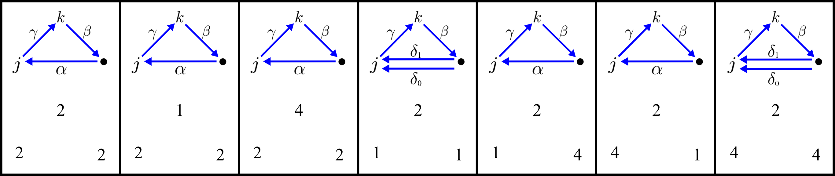
Figure 19.

If $(A,W)$ is a non-degenerate SP, then there exists an $R$-algebra automorphism $\varphi$ of $R\langle\langle A\rangle\rangle$ such that:

(11.2) $$\varphi(W)^{(3)}\sim_{\operatorname{cyc}}\begin{cases}\alpha\beta\gamma&\text{if $(Q,\mathbf{d})$ is the weighted quiver appearing}\\ &\text{in the $1^{\operatorname{st}}$, $2^{\operatorname{nd}}$, $3^{\operatorname{rd}}$, $5^{\operatorname{th}}$ or $6^{\operatorname{th}}$ column of Figure \ref{Fig:3_critical_quivers_2};}\\ \delta_{0}\beta\gamma+\delta_{1}\beta u\gamma&\text{if $(Q,\mathbf{d})$ is the weighted quiver appearing}\\ &\text{in the $4^{\operatorname{th}}$ column of Figure \ref{Fig:3_critical_quivers_2};}\\ (\delta_{0}+\delta_{1})\beta\gamma&\text{if $(Q,\mathbf{d})$ is the weighted quiver appearing}\\ &\text{in the $7^{\operatorname{th}}$ column of Figure \ref{Fig:3_critical_quivers_2}.}\end{cases}$$

Proof.

The lemma follows by verifying that its statement is true for each of the seven weighted quivers in Figure 19. The seven verifications are all very similar, so we include only three of them and leave the remaining four in the hands of the reader.

Case 1.

Suppose that $(Q,\mathbf{d})$ weighted quiver in the $1^{\operatorname{st}}$ column of Figure 19. We claim that $W^{(3)}\not\sim_{\operatorname{cyc}}0$. Indeed, if $W^{(3)}\sim_{\operatorname{cyc}}0$, then the SP $\widetilde{\mu}_{k}(A,W)$ is reduced and hence $\mu_{k}(A,W)=\widetilde{\mu}_{k}(A,W)$; since the underlying species of $\widetilde{\mu}_{k}(A,W)$ is not 2-acyclic, this contradicts the non-degeneracy of $(A,W)$. Therefore, $W^{(3)}\not\sim_{\operatorname{cyc}}0$.

Up to cyclical equivalence, we can write $W^{(3)}=x\alpha\beta\gamma$ for some $x\in L$. The element $x$ is not zero since $W^{(3)}\not\sim_{\operatorname{cyc}}0$. The $R$-algebra automorphism $\varphi$ of $R\langle\langle A\rangle\rangle$ that sends $\alpha$ to $x^{-1}\alpha$ clearly satisfies $\varphi(W)^{(3)}\sim_{\operatorname{cyc}}\alpha\beta\gamma$.

Case 2.

Suppose that $(Q,\mathbf{d})$ weighted quiver in the $4^{\operatorname{th}}$ column of Figure 19. The weighted quiver $\mu_{k}(Q,\mathbf{d})$ is obviously acyclic. Hence, by [27, Theorem 3.24], $(A,W)$ is right-equivalent to $(A,W^{\prime})$, where

$$W^{\prime}=\frac{1}{2}\left(\delta_{1}\beta\gamma+\delta_{0}\beta u^{-1}\gamma\right).$$

The SP $(A,W^{\prime})$ is right-equivalent to $(A,\delta_{1}\beta u\gamma+\delta_{0}\beta\gamma)$ by means of the $R$-algebra automorphism of $R\langle\langle A\rangle\rangle$ that sends $\beta$ to $2\beta u$.

Case 3.

Finally, suppose that $(Q,\mathbf{d})$ weighted quiver in the $7^{\operatorname{th}}$ column of Figure 19. The weighted quiver $\mu_{k}(Q,\mathbf{d})$ is obviously acyclic. Hence, by [27, Theorem 3.24], $(A,W)$ is right-equivalent to $(A,W^{\prime})$, where

$$W^{\prime}=\delta_{0}\beta\gamma+\delta_{1}\beta\gamma.$$

Lemma 11.5 is proved. ∎

Lemma 11.6.

Let ${\mathbf{\Sigma}}=(\Sigma,\mathbb{M},\mathbb{O})$ and $\sigma$ be as in Lemma 11.2, $\omega:\mathbb{O}\rightarrow\{1,4\}$ be any function, and $\zeta\in Z^{1}(\sigma,\omega)$ be any 1-cocycle of the cochain complex $C^{\bullet}(\sigma,\omega)$. If $W\in R\langle\langle A(\sigma,\zeta)\rangle\rangle$ is any non-degenerate potential for $A(\sigma,\zeta)$, then $(A(\sigma,\zeta),W)$ is right-equivalent to $(A(\sigma,\zeta),S(\sigma,\zeta))$.

Proof.

Suppose that $W\in R\langle\langle A(\sigma,\zeta)\rangle\rangle$ is a non-degenerate potential for $A(\sigma,\zeta)$. Let $\triangle$ be an interior triangle of $\sigma$, $i$, $j$ and $k$ be the three arcs of $\sigma$ that are contained in $\triangle$, and $(A(\sigma,\zeta)|_{\triangle},W|_{\triangle})$ be the restriction of $(A(\sigma,\zeta),W)$ to $\{i,j,k\}$ (see [27, Definition 8.1]). The fact that $\sigma$ satisfies the conclusion of Lemma 11.2 implies that the weighted quiver which underlies the species $A(\sigma,\zeta)|_{\triangle}$ is one one of the seven weighted quivers of Figure 19. Since $(A(\sigma,\zeta),W)$ is non-degenerate, $(A(\sigma,\zeta)|_{\triangle},W|_{\triangle})$ is non-degenerate (this is an easy consequence of [27, Lemma 8.2]). Hence, by Lemma 11.5, there exists an $R$-algebra automorphism $\varphi_{\triangle}$ of $R\langle\langle A(\sigma,\zeta)\rangle\rangle$ such that $\varphi_{\triangle}(W|_{\triangle})^{(3)}$ is cyclically equivalent to the right hand side of (11.2).

Assembling all the automorphisms $\varphi_{\triangle}$, with $\triangle$ running in the set of interior triangles of $\sigma$, we obtain an $R$-algebra automorphism $\varphi$ of $R\langle\langle A(\sigma,\zeta)\rangle\rangle$ such that $\varphi(W)^{(3)}\sim_{\operatorname{cyc}}S(\sigma,\zeta)+S^{\prime}$ for some $S^{\prime}\in\mathfrak{m}^{4}$, where $\mathfrak{m}$ is the two-sided ideal of $R\langle\langle A(\sigma,\zeta)\rangle\rangle$ generated by $A(\sigma,\zeta)$.

Since ${\mathbf{\Sigma}}$ is unpunctured, every cyclic path on $A(\sigma,\zeta)$ is cyclically equivalent to a cyclic path that has a factor of the form $bzc$ for some arrows $b$ and $c$ of $Q(\sigma,\omega)$ that are induced by the same triangle and satisfy $t(b)=h(c)$ and $d(\sigma,\omega)_{t(b)}=2$, and some element $z\in\{1,u\}e_{t(b)}\subseteq F_{t(b)}e_{b}$. Using the table depicted in Figure 17, it is not hard to see that $bzc=\sum_{a\in I}\partial_{a}(S(\sigma,\zeta))$ for some non-empty set $I$ consisting of at most two arrows of $Q(\sigma,\zeta)$. Consequently, every cyclic path on $A(\sigma,\zeta)$ is cyclically equivalent to a cyclic path of the form $\sum_{a\in I}\partial_{a}(S(\sigma,\zeta))x_{a}$ for some $x_{a}\in\mathfrak{m}$. Therefore,

$$\varphi(W)^{(3)}\sim_{\operatorname{cyc}}S(\sigma,\zeta)+\sum_{a\in Q_{1}(\sigma,\zeta)}\partial_{a}(S(\sigma,\zeta))x_{a}.$$

A straightforward adaptation of [25, Lemma 8.19 and its proof] shows that there exists an $R$-algebra automorphism $\psi$ of $R\langle\langle A(\sigma,\zeta)\rangle\rangle$ such that $\psi(S(\sigma,\zeta)+\sum_{a\in Q_{1}(\sigma,\zeta)}\partial_{a}(S(\sigma,\zeta))x_{a})\sim_{\operatorname{cyc}}S(\sigma,\zeta)$. Lemma 11.6 is proved. ∎

Corollary 11.7.

Let ${\mathbf{\Sigma}}=(\Sigma,\mathbb{M},\mathbb{O})$ be as in Lemma 11.2, $\omega:\mathbb{O}\rightarrow\{1,4\}$ be any function, and $(\tau,\xi)$ be any colored triangulation of ${\mathbf{\Sigma}_{\omega}}$. If $W\in R\langle\langle A(\tau,\xi)\rangle\rangle$ is any non-degenerate potential for $A(\tau,\xi)$, then $(A(\tau,\xi),W)$ is right-equivalent to $(A(\tau,\xi),S(\tau,\xi))$.

Proof.

This follows from a straightforward combination of Proposition 6.6, Lemmas 11.2 and 11.6, [18, Theorem 4.2], and [27, Theorems 3.21 and 3.24]. For the sake of clarity, we give a detailed argument.

Let $\sigma$ be a triangulation of ${\mathbf{\Sigma}}$ as in Lemma 11.2. By [18, Theorem 4.2], $\sigma$ is related to $\tau$ by a finite sequence of flips. Consequently, there exists a 1-cocycle $\zeta\in Z^{1}(\sigma,\omega)\subseteq C^{1}(\sigma,\omega)$ such that the colored triangulations $(\sigma,\zeta)$ and $(\tau,\xi)$ are related by a finite sequence of colored flips, say $(\sigma,\zeta)=f_{k_{n}}f_{k_{n-1}}\ldots f_{k_{1}}(\tau,\xi)$.

The underlying species of the SP $\mu_{k_{n}}\ldots\mu_{k_{1}}(A(\tau,\xi),W)$ is $A(\sigma,\zeta)$ by Proposition 6.6, so we can write $(A(\sigma,\zeta),W^{\prime})=\mu_{k_{n}}\ldots\mu_{k_{1}}(A(\tau,\xi),W)$. Since $(A(\tau,\xi),W)$ is non-degenerate, $(A(\sigma,\zeta),W^{\prime})$ is non-degenerate too, and therefore, $(A(\sigma,\zeta),W^{\prime})$ is right-equivalent to $(A(\sigma,\zeta),S(\sigma,\zeta))$ by Lemma 11.6.

On the other hand, the SPs $\mu_{k_{n}}\ldots\mu_{k_{1}}(A(\tau,\xi),S(\tau,\xi))$ and $(A(\sigma,\zeta),S(\sigma,\zeta))$ are right-equivalent by Theorem 7.1. Thus, $\mu_{k_{n}}\ldots\mu_{k_{1}}(A(\tau,\xi),S(\tau,\xi))$ is right-equivalent to $(A(\sigma,\zeta),W^{\prime})$. The involutivity of SP-mutations up to right-equivalence, cf. [27, Theorem 3.24], and the fact that SP-mutations send right-equivalent SPs to right-equivalent SPs, cf. [27, Theorem 3.21], imply that $(A(\tau,\xi),S(\tau,\xi))$ is right-equivalent to $\mu_{k_{1}}\ldots\mu_{k_{n}}(A(\sigma,\zeta),W^{\prime})$, SP which is in turn right-equivalent to $(A(\tau,\xi),W)$ by the involutivity of SP-mutations up to right-equivalence. ∎

Putting Corollaries 11.4 and 11.7 together, we obtain the main result of this section, namely:

Theorem 11.8.

Let ${\mathbf{\Sigma}}=(\Sigma,\mathbb{M},\mathbb{O})$ be a surface with marked points and order-2 orbifold points which is unpunctured and different from a torus with exactly one marked point and without orbifold points, $\omega:\mathbb{O}\rightarrow\{1,4\}$ any function, $\tau$ any triangulation of ${\mathbf{\Sigma}}$, $F$ any field containing a primitive $d^{\operatorname{th}}$ root of unity, where $d=\operatorname{lcm}(\mathbf{d}(\tau,\omega))$, and $E/F$ any degree-$d$ cyclic Galois extension. Any realization of the skew-symmetrizable matrix $B(\tau,\omega)$ via a non-degenerate SP over $E/F$ is right-equivalent to $(A(\tau,\xi),S(\tau,\xi))$ for some 1-cocycle $\xi\in Z^{1}(\tau,\omega)\subseteq C^{1}(\tau,\omega)$.

12. Some problems

Conjecture 12.1.

If ${\mathbf{\Sigma}}$ admits a triangulation $\sigma$ such that the quiver $\overline{Q}(\sigma)$ (equivalently, any of the quivers $Q(\sigma,\omega)$ for $\omega:\mathbb{O}\rightarrow\{1,4\}$) is acyclic, then for any function $\omega:\mathbb{O}\rightarrow\{1,4\}$, and any colored triangulation $(\rho,\xi)$ of ${\mathbf{\Sigma}_{\omega}}$, the Jacobian algebra $\mathcal{P}((A(\rho,\xi),S(\rho,\xi)))$ is cluster-tilted in the sense [8, 9] of Buan-Marsh-Reineke-Reiten-Todorov and Buan-Marsh-Reiten. More precisely, we conjecture that for $(\rho,\xi)$ there is a 1-cocycle $\zeta\in Z(\sigma,\omega)$ such that $\mathcal{P}((A(\rho,\xi),S(\rho,\xi)))$ is isomorphic as an $F$-algebra to the endomorphism algebra of a cluster-tilting object of the orbit category $\mathcal{D}/(\tau^{-1}\circ[1])$, where $\mathcal{D}$ is the bounded derived category of the module category of the hereditary algebra $\mathcal{P}((A(\sigma,\zeta),S(\sigma,\zeta)))$ (note that $S(\sigma,\zeta)=0$ by the acyclicity of $\overline{Q}(\sigma)$), and $\tau$ and $[1]$ are the Auslander-Reiten translation and the shift functor of $\mathcal{D}$, respectively.

Question 12.2.

Can the results of Amiot [1, 2], Keller-Yang [28] and Plamondon [36, 37] be applied or adapted in order to be able to associate 2- and 3-Calabi-Yau triangulated categories to the surfaces ${\mathbf{\Sigma}_{\omega}}=(\Sigma,\mathbb{M},\mathbb{O},\omega)$ treated in [27] and in this paper?

Problem 12.3.

Given an arbitrarily punctured surface ${\mathbf{\Sigma}}=(\Sigma,\mathbb{M},\mathbb{O})$ with order-2 orbifold points, and an arbitrary function $\omega:\mathbb{O}\rightarrow\{1,4\}$, determine whether it is possible to associate species with potential to the (colored) triangulations of ${\mathbf{\Sigma}_{\omega}}$, in such a way that the SPs associated to (colored) triangulations related by a (colored) flip are correspondingly related by the SP-mutation defined in [27, Definitions 3.19 and 3.22].

Question 12.4.

Let ${\mathbf{\Sigma}}=(\Sigma,\mathbb{M},\mathbb{O})$ be either unpunctured or once-punctured closed, and let $\omega:\mathbb{O}\rightarrow\{1,4\}$ be any function. Can the cluster algebra associated to ${\mathbf{\Sigma}_{\omega}}$ by Felikson-Shapiro-Tumarkin be realized as a suitable Caldero-Chapoton algebra of the Jacobian algebras of the colored triangulations of ${\mathbf{\Sigma}_{\omega}}$ (see [11])? More precisely, is it possible to define a Caldero-Chapoton algebra for the Jacobian algebra of each colored triangulation of ${\mathbf{\Sigma}_{\omega}}$, in such a way that it turns out to be independent of the colored triangulation chosen and sits between the upper cluster algebra and the cluster algebra associated to ${\mathbf{\Sigma}_{\omega}}$ with respect to some choice of coefficient system?

In [13], Chekhov-Shapiro have associated a generalized cluster algebra to each surface with marked points and orbifold points of arbitrary order. The cluster mutation rule inside a generalized cluster algebra differs from that of a cluster algebra in that it allows its exchange polynomials to not be binomials, while in a cluster algebra all exchange polynomials are binomials. The (algebraic) combinatorics of generalized cluster algebras is very similar to the combinatorics of cluster algebras, though. For instance, they possess the remarkable Laurent phenomenon.

Question 12.5.

Can the generalized cluster algebras of Chekhov-Shapiro be realized as Caldero-Chapoton algebras of (suitably constructed) associative algebras?

13. Examples

13.1. Types $\mathbb{A}_{n}$, $\mathbb{C}_{n}$, $\widetilde{\mathbb{C}}_{n}$, $\mathbb{B}_{n}$, $\widetilde{\mathbb{B}}_{n}$ and $\widetilde{\mathbb{BC}}_{n}$ via polygons with at most two orbifold points

Let us say that the matrices

$B=\left[\begin{array}[]{rrrrrr}0&-2&0&&0&0\\ 1&0&-1&\ldots&0&0\\ 0&1&0&&0&0\\ &\vdots&&\ddots&&\\ 0&0&0&&0&-1\\ 0&0&0&&1&0\end{array}\right]\in\mathbb{Z}^{(n-1)\times(n-1)}$,	$\widetilde{B}=\left[\begin{array}[]{rrrrrrr}0&-2&0&&0&0&0\\ 1&0&-1&\ldots&0&0&0\\ 0&1&0&&0&0&0\\ &\vdots&&\ddots&&&\\ 0&0&0&&0&-1&0\\ 0&0&0&&1&0&-1\\ 0&0&0&&0&2&0\end{array}\right]\in\mathbb{Z}^{(n+1)\times(n+1)}$,
$C=\left[\begin{array}[]{rrrrrr}0&-1&0&&0&0\\ 2&0&-1&\ldots&0&0\\ 0&1&0&&0&0\\ &\vdots&&\ddots&&\\ 0&0&0&&0&-1\\ 0&0&0&&1&0\end{array}\right]\in\mathbb{Z}^{(n-1)\times(n-1)}$,	$\widetilde{C}=\left[\begin{array}[]{rrrrrrr}0&-1&0&&0&0&0\\ 2&0&-1&\ldots&0&0&0\\ 0&1&0&&0&0&0\\ &\vdots&&\ddots&&&\\ 0&0&0&&0&-1&0\\ 0&0&0&&1&0&-2\\ 0&0&0&&0&1&0\end{array}\right]\in\mathbb{Z}^{(n+1)\times(n+1)}$,
$X=\left[\begin{array}[]{rrrrrrr}0&-1&0&&0&0\\ 1&0&-1&\ldots&0&0\\ 0&1&0&&0&0\\ &\vdots&&\ddots&&\\ 0&0&0&&0&-1\\ 0&0&0&&1&0\end{array}\right]\in\mathbb{Z}^{(n-3)\times(n-3)}$    and	$\widetilde{Y}=\left[\begin{array}[]{rrrrrrr}0&-2&0&&0&0&0\\ 1&0&-1&\ldots&0&0&0\\ 0&1&0&&0&0&0\\ &\vdots&&\ddots&&&\\ 0&0&0&&0&-1&0\\ 0&0&0&&1&0&-2\\ 0&0&0&&0&1&0\end{array}\right]\in\mathbb{Z}^{(n+1)\times(n+1)}$

are of type $\mathbb{B}_{n-1}$ $(n\geq 3)$, $\widetilde{\mathbb{B}}_{n}$ ($n\geq 2$), $\mathbb{C}_{n-1}$ ($n\geq 3$), $\widetilde{\mathbb{C}}_{n}$ ($n\geq 2$), $\mathbb{A}_{n-3}$ ($n\geq 4$) and $\widetilde{\mathbb{BC}}_{n}$ ($n\geq 2$), respectively. These matrices can respectively be skew-symmetrized by

$D_{\mathbb{B}}=\operatorname{diag}(1,2,2\ldots,2,2)$,	$D_{\widetilde{\mathbb{B}}}=\operatorname{diag}(1,2,2\ldots,2,2,1)$,
$D_{\mathbb{C}}=\operatorname{diag}(4,2,2,\ldots,2,2)$,	$D_{\widetilde{\mathbb{C}}}=\operatorname{diag}(4,2,2,\ldots,2,2,4)$,
$D_{\mathbb{A}}=\operatorname{diag}(2,2,2,\ldots,2,2)$    and	$D_{\widetilde{\mathbb{BC}}}=\operatorname{diag}(1,2,2,\ldots,2,2,4)$,

The weighted quivers corresponding under [32, Lemma 2.3] to the pairs $(B,D_{\mathbb{B}})$, $(\widetilde{B},D_{\widetilde{\mathbb{B}}})$, $(C,D_{\mathbb{C}})$, $(\widetilde{C},D_{\widetilde{\mathbb{C}}})$, $(X,D_{\mathbb{A}})$ and $(Y,D_{\widetilde{\mathbb{BC}}})$ are

$(Q_{B},\mathbf{d}_{\mathbb{B}})$	$=$	$(1\to 2\to 3\ldots\to n-2\to n-1,$	$1\ \ 2\ \ 2\ \ \ldots\ \ 2\ \ 2)$,
$(Q_{\widetilde{B}},\mathbf{d}_{\widetilde{\mathbb{B}}})$	$=$	$(1\to 2\to 3\ldots\to n-1\to n\to n+1,$	$1\ \ 2\ \ 2\ \ \ldots\ \ 2\ \ 2\ \ 1)$,
$(Q_{C},\mathbf{d}_{\mathbb{C}})$	$=$	$(1\to 2\to 3\ldots\to n-2\to n-1,$	$4\ \ 2\ \ 2\ \ \ldots\ \ 2\ \ 2)$,
$(Q_{\widetilde{C}},\mathbf{d}_{\widetilde{\mathbb{C}}})$	$=$	$(1\to 2\to 3\ldots\to n-1\to n\to n+1,$	$4\ \ 2\ \ 2\ \ \ldots\ \ 2\ \ 2\ \ 4)$,
$(Q_{X},\mathbf{d}_{\mathbb{A}})$	$=$	$(1\to 2\to 3\ldots\to n-4\to n-3,$	$2\ \ 2\ \ 2\ \ \ldots\ \ 2\ \ 2)$,
and    $(Q_{\widetilde{Y}},\mathbf{d}_{\widetilde{\mathbb{BC}}})$	$=$	$(1\to 2\to 3\ldots\to n-1\to n\to n+1,$	$1\ \ 2\ \ 2\ \ \ldots\ \ 2\ \ 2\ \ 4)$.

Example 13.1.

Let ${\mathbf{\Sigma}}=(\Sigma,\mathbb{M},\mathbb{O})$ be an $n$-gon with exactly one orbifold point $q$ (that is, $\mathbb{O}=\{q\}$), and let $\omega_{\mathbb{B}},\omega_{\mathbb{C}}:\mathbb{O}\rightarrow\{1,4\}$ be the functions given by $\omega_{\mathbb{B}}(q)=1$ and $\omega_{\mathbb{C}}(q)=4$. Then the weighted quivers $(Q_{B},\mathbf{d}_{\mathbb{B}})$ and $(Q_{C},\mathbf{d}_{\mathbb{C}})$ respectively coincide with $(Q(\tau,\omega_{\mathbb{B}}),\mathbf{d}(\tau,\omega_{\mathbb{B}}))$ and $(Q(\tau,\omega_{\mathbb{C}}),\mathbf{d}(\tau,\omega_{\mathbb{C}}))$, where $\tau$ is the following triangulation of ${\mathbf{\Sigma}}$:

Example 13.2.

Let ${\mathbf{\Sigma}}=(\Sigma,\mathbb{M},\mathbb{O})$ be an $n$-gon with exactly two orbifold points $q_{1}$ and $q_{2}$ (that is, $\mathbb{O}=\{q_{1},q_{2}\}$), and let $\omega_{\widetilde{\mathbb{B}}},\omega_{\widetilde{\mathbb{C}}},\omega_{\widetilde{\mathbb{BC}}}:\mathbb{O}\rightarrow\{1,4\}$ be the functions given by $\omega_{\widetilde{\mathbb{B}}}(q_{1})=1=\omega_{\widetilde{\mathbb{B}}}(q_{2})$, $\omega_{\widetilde{\mathbb{C}}}(q_{1})=4=\omega_{\widetilde{\mathbb{C}}}(q_{2})$, $\omega_{\widetilde{\mathbb{BC}}}(q_{1})=1$ and $\omega_{\widetilde{\mathbb{BC}}}(q_{2})=4$ Then the weighted quivers $(Q_{\widetilde{B}},\mathbf{d}_{\widetilde{\mathbb{B}}})$, $(Q_{\widetilde{C}},\mathbf{d}_{\widetilde{\mathbb{C}}})$ and $(Q_{\widetilde{Y}},\mathbf{d}_{\widetilde{\mathbb{BC}}})$ respectively coincide with $(Q(\tau,\omega_{\widetilde{\mathbb{B}}}),\mathbf{d}(\tau,\omega_{\widetilde{\mathbb{B}}}))$, $(Q(\tau,\omega_{\widetilde{\mathbb{C}}}),\mathbf{d}(\tau,\omega_{\widetilde{\mathbb{C}}}))$ and $(Q(\tau,\omega_{\widetilde{\mathbb{BC}}}),\mathbf{d}(\tau,\omega_{\widetilde{\mathbb{BC}}}))$, where $\tau$ is the following triangulation of ${\mathbf{\Sigma}}$:

Example 13.3.

Let ${\mathbf{\Sigma}}=(\Sigma,\mathbb{M},\mathbb{O})$ be an $n$-gon without orbifold points (that is, $\mathbb{O}=\varnothing$), and let $\omega_{\mathbb{A}}:\mathbb{O}\rightarrow\{1,4\}$ be the empty function. Then the weighted quiver $(Q_{X},\mathbf{d}_{\mathbb{A}})$ coincides with $(Q(\tau,\omega_{\mathbb{A}}),\mathbf{d}(\tau,\omega_{\mathbb{A}}))$, where $\tau$ is the following triangulation of ${\mathbf{\Sigma}}$:

Using Examples 13.1, 13.2 and 13.3, we see that any matrix $B^{\prime}$ mutation-equivalent to a matrix of type $\mathbb{B}_{n-1}$, $\widetilde{\mathbb{B}}_{n}$, $\mathbb{C}_{n-1}$, $\widetilde{\mathbb{C}}_{n}$, $\mathbb{A}_{n-3}$ or $\widetilde{\mathbb{BC}}_{n}$, is the matrix associated by Felikson-Shapiro-Tumarkin to a triangulation $\sigma$ of a polygon with at most two orbifold points with respect to some function $\omega$. Whenever we choose an arbitrary 1-cocycle $\zeta\in Z^{1}(\sigma,\omega)$, we obtain an SP-realization of $B^{\prime}$ via the non-degenerate SP $(A(\sigma,\zeta),S(\sigma,\zeta))$. Note that, by Theorem 10.1, the isomorphism class of $\mathcal{P}(A(\sigma,\zeta),S(\sigma,\zeta))$ as an $F$-algebra is independent of the chosen cocycle $\zeta$ since $H^{1}(C^{\bullet}(\sigma,\omega))$ is isomorphic to the first singular cohomology group of a disc (with coefficients in $\mathbb{F}_{2}$).

As stated in Conjecture 12.1, we believe that the Jacobian algebra $\mathcal{P}(A(\sigma,\zeta),S(\sigma,\zeta))$ is cluster-tilted in the sense [8] of Buan-Marsh-Reineke-Reiten-Todorov. Thus, for instance, we believe the algebras from Examples 6.3 and 6.4 to be cluster-tilted of types $\mathbb{C}_{5}$ and $\widetilde{\mathbb{C}}_{5}$, respectively.

Example 13.4.

Let ${\mathbf{\Sigma}}=(\Sigma,\mathbb{M},\mathbb{O})$ be the unpunctured hexagon with exactly one orbifold point $q$, $\omega:\mathbb{O}\rightarrow\{1,4\}$ be the function that takes the value $1$ at $q$, and $\tau$ be the triangulation of ${\mathbf{\Sigma}}$ depicted in Figure 12. Take $\mathbb{C}/\mathbb{R}$ as the ground field extension $E/F$. If $\xi\in Z^{1}(\tau,\omega)$ is the zero cocycle, then the semisimple ring $R=\bigoplus_{k\in\tau}F_{k}$ and the species $A(\tau,\xi)$ can be (informally) visualized as follows:

Furthermore, $\mathbb{R}$ sits as a central subring of the Jacobian algebra $\mathcal{P}(A(\tau,\xi),S(\tau,\xi))$, and the following identities hold in $\mathcal{P}(A(\tau,\xi),S(\tau,\xi))$:

$$\alpha z=z\alpha,\ \beta z=z\beta,\ \gamma z=z\gamma,\ \delta z=z\delta,\ \text{for all $z\in\mathbb{C}$},$$

$$\beta\gamma=\gamma\alpha=\alpha\beta=\eta\nu=\nu\delta=\delta\eta=0.$$

Since $H^{1}(C^{\bullet}(\tau,\omega))\cong H^{1}(\Sigma;\mathbb{F}_{2})$ is zero, Theorem 10.1 implies that for any 1-cocycle $\xi^{\prime}\in Z^{1}(\tau,\omega)$ the Jacobian algebra $\mathcal{P}(A(\tau,\xi^{\prime}),S(\tau,\xi^{\prime}))$ will be isomorphic to $\mathcal{P}(A(\tau,\xi),S(\tau,\xi))$ as an $\mathbb{R}$-algebra (of course, provided we do not decide to change our ground field extension $E/F$ all of the sudden). As we have said in Conjecture 12.1, we believe $\mathcal{P}(A(\tau,\xi),S(\tau,\xi))$ to be a cluster-tilted algebra of type $\mathbb{B}_{5}$.

13.2. Two non-isomorphic algebras for the Kronecker quiver

Let ${\mathbf{\Sigma}}=(\Sigma,\mathbb{M},\mathbb{O})$ be an unpunctured annulus with exactly two marked points (one on each boundary component) and without orbifold points, let $\omega:\mathbb{O}\rightarrow\{1,4\}$ be the empty function, and let $\tau=\{j_{1},j_{2}\}$ be any triangulation of ${\mathbf{\Sigma}}$. Then $\overline{Q}(\tau)=Q(\tau,\omega)=Q^{\prime}(\tau,\omega)=Q^{\prime\prime}(\tau,\omega)$ has exactly two arrows, say $a:j_{1}\rightarrow j_{2}$ and $b:j_{1}\rightarrow j_{2}$, and we clearly have $X_{2}(\tau,\omega)=\varnothing$. Hence $\dim_{\mathbb{F}_{2}}(C^{1}(\tau,\omega))=2$ and every element $\xi\in C^{1}(\tau,\omega)$ is a 1-cocycle. Let $\{\xi_{a},\xi_{b}\}$ be the $\mathbb{F}_{2}$-vector space basis of $C^{1}(\tau,\omega)$ which is $\mathbb{F}_{2}$-dual to the $\mathbb{F}_{2}$-basis $\{a,b\}$ of $C_{1}(\tau,\omega)$. Then $C^{1}(\tau,\omega)=\{0,\xi_{a},\xi_{b},\xi_{a}+\xi_{b}\}$.

Let us take $\mathbb{C}/\mathbb{R}$ as our ground field extension. It is fairly easy to check that $\mathcal{P}(A(\tau,0),S(\tau,0))\cong\mathcal{P}(A(\tau,\xi_{a}+\xi_{b}),S(\tau,\xi_{a}+\xi_{b}))\not\cong\mathcal{P}(A(\tau,\xi_{a}),S(\tau,\xi_{a}))\cong\mathcal{P}(A(\tau,\xi_{b}),S(\tau,\xi_{b}))$ as rings and as $\mathbb{R}$-algebras. It is also easy to directly verify that $[0]=[\xi_{a}+\xi_{b}]$ and $[\xi_{a}]=[\xi_{b}]$ as elements of $H^{1}(C^{\bullet}(\tau,\omega))$. This is in sync with Theorem 10.1.

As the reader can readily check, the field $\mathbb{C}$ acts centrally on the ring $\mathcal{P}(A(\tau,0),S(\tau,0))$, and $\mathcal{P}(A(\tau,0),S(\tau,0))$ is isomorphic, as a $\mathbb{C}$-algebra, to the usual path algebra over $\mathbb{C}$ of the well-known Kronecker quiver. On the other hand, the right and left actions of $\mathbb{C}$ on $\mathcal{P}(A(\tau,\xi_{a}),S(\tau,\xi_{a}))$ are related by the identities

$$az=\theta(z)a\ \ \ \text{and}\ \ \ bz=zb,$$

which hold for all $z\in\mathbb{C}$, where $\theta:\mathbb{C}\rightarrow\mathbb{C}$ is the usual conjugation of complex numbers. This means that if $M$ is a left $\mathcal{P}(A(\tau,\xi_{a}),S(\tau,\xi_{a}))$-module, and if we set $M_{j_{1}}=e_{j_{1}}M$, $M_{j_{2}}=e_{j_{2}}$, $M_{a},M_{b}:M_{j_{1}}\rightarrow M_{j_{2}}$, $M_{a}(m)=am$, $M_{b}(m)=b_{m}$, then $M_{j_{1}}$ and $M_{j_{2}}$ are $\mathbb{C}$-vector spaces, $M_{b}$ is a $\mathbb{C}$-linear transformation and $M_{a}$ is an $\mathbb{R}$-linear transformation which is not $\mathbb{C}$-linear (unless $M_{a}=0$) but rather satisfies $M_{a}(zm)=\theta(z)M_{a}(m)$ for $z\in\mathbb{C}$ and $m\in M_{j_{1}}$. In particular, the category of left $\mathcal{P}(A(\tau,\xi_{a}),S(\tau,\xi_{a}))$-modules is not equal to the well-known category of left modules over the usual path algebra over $\mathbb{C}$ of the Kronecker quiver. A little effort shows that, actually, these two categories are not equivalent as additive categories. Indeed, in $\mathcal{P}(A(\tau,0),S(\tau,0))$-$\operatorname{mod}$ every non-zero endomorphism ring has $\mathbb{C}$ as a subring, but at least one object of $\mathcal{P}(A(\tau,\xi_{a}),S(\tau,\xi_{a}))$-$\operatorname{mod}$ has $\mathbb{R}$ as its endomorphism ring, and $\mathbb{R}$ has no subring isomorphic to $\mathbb{C}$, so an additive equivalence between the two categories cannot exist.

The classification of the indecomposable $\mathcal{P}(A(\tau,\xi_{a}),S(\tau,\xi_{a}))$-modules has been carried out in [16].

13.3. Relation to previous constructions

Suppose that ${\mathbf{\Sigma}}=(\Sigma,\mathbb{M},\mathbb{O})$ is unpunctured and that $\omega:\mathbb{O}\rightarrow\{1,4\}$ is the constant function that takes the value $4$ at every element of $\mathbb{O}$. Then for any two triangulations $\tau$ and $\sigma$ of ${\mathbf{\Sigma}}$ that are related by the flip of an arc $k\in\tau$, the function $Z^{1}(\tau,\omega)\rightarrow Z^{1}(\sigma,\omega)$ given by the colored flip is $\mathbb{F}_{2}$-linear. Therefore, if $(\tau,\xi)$ is a colored triangulation such that $\xi\in Z^{1}(\tau,\omega)$ is the zero cocycle, then applying any finite sequence of colored flips to $(\tau,\xi)$ will always produce a colored triangulation $(\rho,\zeta)$ whose underlying cocycle $\zeta$ is the zero cocycle (in the corresponding cochain complex $C^{\bullet}(\rho,\omega)$). This means that if $\omega$ never takes the value $1$, then neither colored flips nor SP-mutations obstruct us if we decide to always choose the zero cocycle.

Example 13.5.

Suppose that $\mathbb{O}=\varnothing$, so that $\omega$ is actually the empty function. If $(\tau,\xi)$ is a colored triangulation of ${\mathbf{\Sigma}_{\omega}}$ such that $\xi=0$, and $\mathbb{C}/\mathbb{R}$ is our ground field extension (note that $d(\tau,\omega)_{k}=2$ for every $k\in\tau$ since $\mathbb{O}=\varnothing$), then $\mathbb{C}$ acts centrally on the path algebra $R\langle A(\tau,\xi)\rangle$, on the complete path algebra $R\langle\langle A(\tau,\xi)\rangle\rangle$ and on the Jacobian algebra $\mathcal{P}(A(\tau,\xi),S(\tau,\xi))$ (which means that these rings are $\mathbb{C}$-algebras and not only $\mathbb{R}$-algebras), and the SP $(A(\tau,\xi),S(\tau,\xi))$ coincides with the quiver with potential defined in [30, 31]. The fact that ${\mathbf{\Sigma}}$ is unpunctured implies then that $\mathcal{P}(A(\tau,\xi),S(\tau,\xi))$ is the gentle algebra studied in [6] by Assem-Brüstle-Charbonneau-Plamondon.

Example 13.6.

Suppose that $\mathbb{O}\neq\varnothing$. If $\tau$ is any triangulation of ${\mathbf{\Sigma}}$, then $d(\tau,\omega)_{k}\in\{2,4\}$ for every $k\in\tau$, and so, Section 6 tells us that our ground field extension should have degree $4$. However, if $\xi=0\in Z^{1}(\tau,\omega)$, then we can actually work with a degree-2 extension $E/L$ of fields of characteristic different from $2$ (for example, $\mathbb{C}/\mathbb{R}$). Indeed, if $\xi=0$, then we can set $g(\tau,\xi)_{\alpha}=11_{L}$ for every arrow $\alpha$ incident to at least one non-pending arc, and

$$g(\tau,\xi)_{\alpha}=\begin{cases}11_{E}&\text{if $\alpha=\delta_{0}^{\triangle}$;}\\ \vartheta&\text{if $\alpha=\delta_{1}^{\triangle}$;}\end{cases}$$

for every twice-orbifolded triangle $\triangle$ of $\tau$, where $\vartheta$ is the non-identity element of $\operatorname{Gal}(E/L)$, and the arrows $\delta_{0}^{\triangle}$ and $\delta_{1}^{\triangle}$ are defined as in item (3) of Definition 6.1 for such a triangle $\triangle$. The SP obtained in this way coincides with the SP defined in [27]. This means that for unpunctured surfaces, the SPs constructed in this paper generalize those constructed in [27].

14. Proof of Theorem 7.1

Proof of Theorem 7.1.

Consider the three puzzle pieces shown in Figure 20.

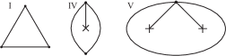
Figure 20. Unpunctured puzzle pieces

Since ${\mathbf{\Sigma}}$ is either unpunctured or once-punctured closed, a consequence of [27, Theorem 2.7] is that both $\tau$ and $\sigma$ have puzzle-piece decompositions that involve only puzzle pieces of types I, IV or V. Fix such a puzzle-piece decomposition of $\tau$. The arc $k\in\tau$ is then either a pending arc inside a puzzle piece or an arc shared by two puzzle pieces. Figure 21 lists the three possibilities for $k$ if $k$ happens to be a pending arc, while Figure 22 lists all the possibilities for $k$ if $k$ happens to be an arc shared by two puzzle pieces.

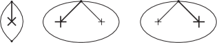
Figure 21.

$$\vbox{ \leavevmode\hbox to62.75pt{\vbox to68.34pt{\text{[drawing]}}} }\begin{array}[]{cccc}\leavevmode\hbox to64.92pt{\vbox to69.17pt{\text{[drawing]}}}&\leavevmode\hbox to68.84pt{\vbox to69.17pt{\text{[drawing]}}}&\leavevmode\hbox to52.18pt{\vbox to69.17pt{\text{[drawing]}}}&\leavevmode\hbox to68.84pt{\vbox to69.17pt{\text{[drawing]}}}\\ \leavevmode\hbox to64.92pt{\vbox to69.17pt{\text{[drawing]}}}&\leavevmode\hbox to68.84pt{\vbox to69.17pt{\text{[drawing]}}}&\leavevmode\hbox to52.18pt{\vbox to69.17pt{\text{[drawing]}}}&\leavevmode\hbox to68.84pt{\vbox to69.17pt{\text{[drawing]}}}\end{array} \bullet \bullet \bullet \times i j l k \bullet \bullet \times \times i j k j \bullet \times \times \times i k j \bullet \bullet \times \times i j k j \bullet \bullet \bullet \times i j l k \bullet \bullet \times \times i j k j \bullet \times \times \times i k j \bullet \bullet \times \times i j k j \bullet \bullet \bullet \times i j l k \bullet \bullet \times \times i j k j \bullet \times \times \times i k j \bullet \bullet \times \times i j k j \bullet \bullet \bullet \times i j l k \bullet \bullet \times \times i j k j \bullet \times \times \times i k j \bullet \bullet \times \times i j k j$$

Figure 22.

Note that each of the sides $i,j,l,m$ of the configurations depicted in Figure 22 may be either an arc of $\tau$ or a boundary segment.

We will prove Theorem 7.1 by showing that its assertion is true for each of the three configurations depicted in Figure 21 and each of the nine configurations depicted in Figure 22. Now, all but one of these twelve configurations involve at least one (and at most three) orbifold point. Since $\omega$ is an arbitrary function from $\mathbb{O}$ to $\{1,4\}$, this means that for each configuration, if it involves $\nu$ orbifold points ($0\leq\nu\leq 3$), we have to take into account the $2^{\nu}$ possible combinations of values that $\omega$ can take on the $\nu$ orbifold points involved. This gives us a total of $47=(2+4+4)+(1+2+2+4+4+8+8+4+4)$ possible cases to take into account; these cases have been depicted in Figure 23.

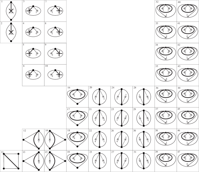
Figure 23.

However, note that in Figure 23 the following pairs of configurations correspond to each other under the flip of $k$:

$$\begin{array}[]{cccc}3\leftrightarrow 7&4\leftrightarrow 9&5\leftrightarrow 8&6\leftrightarrow 10\\ 12\leftrightarrow 14&13\leftrightarrow 15&16\leftrightarrow 20&17\leftrightarrow 21\\ 18\leftrightarrow 22&19\leftrightarrow 23&24\leftrightarrow 28&25\leftrightarrow 30\\ 26\leftrightarrow 29&27\leftrightarrow 31&32\leftrightarrow 40&33\leftrightarrow 44\\ 34\leftrightarrow 41&35\leftrightarrow 45&36\leftrightarrow 42&37\leftrightarrow 46\\ &38\leftrightarrow 43&39\leftrightarrow 47.&\end{array}$$

Note also that configuration 25 coincides with configuration 26. Since flips and SP-mutations are involutive (the latter up to right-equivalence, cf. [27, Theorem 3.24]), this means that, in order to know that the statement of Theorem 7.1 is true for the 47 configurations of Figure 23, it suffices to show it is true for the following 24 configurations:

$$\begin{array}[]{ccccc}1&2&3&4&5\\ 6&11&12&13&20\\ 21&22&23&24&25\\ \phantom{26}&27&32&33&34\\ 35&36&37&38&39.\end{array}$$

This is what we will do. In all the 24 cases, the strategy we shall adopt is the following:

1. Draw $\tau$ and $\sigma$, and draw the quivers $Q(\tau,\xi)$ and $\widetilde{\mu}_{k}(Q(\tau,\xi))$ on top of $\tau$ and $\sigma$, respectively.The elements of certain set of arrows whose removal from $\widetilde{\mu}_{k}(Q(\tau,\xi))$ gives (a quiver isomorphic to) $\mu_{k}(Q(\tau,\xi))$ will be drawn as dotted arrows. We will identify $Q(\sigma,\zeta)$ with the subquiver of $\widetilde{\mu}_{k}(Q(\tau,\xi))$ obtained by deleting the dotted arrows. This identification will have the property that for every arrow $a$ of $Q(\sigma,\zeta)$, the value of the modulating function $g(\sigma,\zeta)$ at $a$ coincides with the value of $\widetilde{\mu}_{k}(g(\tau,\xi))$ at $a$. [This property, whose verification we will leave in the hands of the reader in all cases, will be an easy consequence of the definition of $\widetilde{\mu}_{k}(g(\tau,\xi))$, the definition of flips of colored triangulations (recall that we have $(\sigma,\zeta)=f_{k}(\tau,\xi)$ by hypothesis), and the definition of $g(\sigma,\zeta)$.] The 1-cocycles $\xi$ and $\zeta$ will not be indicated in the figures.

2. Define certain potential $S(\sigma,\zeta)^{\sharp}\in R\langle\langle\widetilde{\mu}_{k}(A(\tau,\xi))\rangle\rangle$ as the sum of $S(\sigma,\zeta)$ and a degree-2 potential on $\widetilde{\mu}_{k}(A(\tau,\xi))$. The SP $(\widetilde{\mu}_{k}(A(\tau,\xi)),S(\sigma,\zeta)^{\sharp})$ will have the property of having $(A(\sigma,\zeta),S(\sigma,\zeta))$ as a reduced part. [This property will be a consequence of the fact that every 2-cycle $ab$ appearing in (the degree-2 component of) $S(\sigma,\zeta)^{\sharp}$ will satisfy $\widetilde{\mu}_{k}(g(\tau,\xi))(a)=\left(\widetilde{\mu}_{k}(g(\tau,\xi))(b)\right)^{-1}$. This fact, whose verification we will leave in the hands of the reader in all cases, is an easy consequence of the definition of $\widetilde{\mu}_{k}(g(\tau,\xi))$ and of the fact that $\xi$ is a $1$-cocycle in the cochain complex $C^{\bullet}(\tau,\omega)$.]

3. Write down $S(\tau,\xi)$ and a potential cyclically equivalent to $\widetilde{\mu}_{k}(S(\tau,\xi))$ explicitly. The potential cyclically equivalent to $\widetilde{\mu}_{k}(S(\tau,\xi))$ will always be the result of applying the following fact to some of the summands of $\widetilde{\mu}_{k}(S(\tau,\xi))$: For any arrow $a:j\rightarrow i$ and any element $x$ of the complete path algebra, if $xa$ is a potential, then $xa\sim_{\operatorname{cyc}}\pi_{g_{a}^{-1}}(x)a$, where $\pi_{g_{a}^{-1}}(x)=\frac{1}{d_{i,j}}\sum_{\omega\in\mathcal{B}_{i,j}}g_{a}^{-1}(\omega^{-1})x\omega$ (this is proved in [27, Example 3.12]).

4. Exhibit a finite sequence of explicitly-defined $R$-algebra automorphisms of $R\langle\langle\widetilde{\mu}_{k}(A(\tau,\xi))\rangle\rangle$ with the property that its composition sends $\widetilde{\mu}_{k}(S(\tau,\xi))$ to a potential which is cyclically equivalent to $S(\sigma,\zeta)^{\sharp}$. The fact that the automorphisms in the sequence are indeed well defined will be a consequence of the definition of $\widetilde{\mu}_{k}(g(\tau,\xi))$ and of the fact that $\xi$ is a $1$-cocycle in the cochain complex $C^{\bullet}(\tau,\omega)$. The property that the composition of these automorphisms sends $\widetilde{\mu}_{k}(S(\tau,\xi))$ to a potential cyclically equivalent to $S(\sigma,\zeta)^{\sharp}$ will follow from direct computation; we will omit this computation.

Note that once we have this last step, that is, once we know that $\widetilde{\mu}_{k}(A(\tau,\xi),S(\tau,\xi))$ is right-equivalent to $(\widetilde{\mu}_{k}(A(\tau,\xi),S(\sigma,\zeta)^{\sharp})$, it will follow from [27, Theorem 3.16] that $\mu_{k}((A(\tau,\xi),S(\tau,\xi)))$ is right-equivalent to $(A(\sigma,\zeta),S(\sigma,\zeta))$.

Remark 14.1.

1. In order to keep the notation as light as possible throughout the proof, we will write $g$ for the modulating function $g(\tau,\xi)$ and $\widetilde{\mu}_{k}(g)$ for the modulating function $\widetilde{\mu}_{k}(g(\tau,\xi))$.

2. It is easy to deduce from [27, Example 3.12] that whenever we have an arrow $a:j\rightarrow i$ of $\widetilde{\mu}_{k}(A(\tau,\xi))$ and an element $x\in e_{j}R\langle\langle\widetilde{\mu}_{k}(A(\tau,\xi))\rangle\rangle e_{i}$, we necessarily have $xa\sim_{\operatorname{cyc}}\pi_{(\widetilde{\mu}_{k}(g)_{a})^{-1}}(x)a$, where $\widetilde{\mu}_{k}(g)_{a}$ is the value of the modulating function $\widetilde{\mu}_{k}(g)$ at $a$ (see [27, Definition 3.19]) and $\pi_{(\widetilde{\mu}_{k}(g)_{a})^{-1}}(x):=\frac{1}{d_{i,j}}\sum_{\omega\in\mathcal{B}_{i,j}}(\widetilde{\mu}_{k}(g)_{a})^{-1}(\omega^{-1})x\omega$. We will use this fact repeatedly throughout the proof without any further apology ($a$ will usually be a composite arrow of $\widetilde{\mu}_{k}(A(\tau,\xi))$).

Case 1.

Configuration 1.

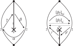
Figure 24. First configuration of Figure 23. Left: $\tau$ and $Q(\tau,\omega)$. Right: $\sigma$ and $\widetilde{\mu}_{k}(Q(\tau,\omega))$. The numbers next to the arcs are the corresponding values of the tuple $\mathbf{d}(\tau,\omega)$.

1. We use the notation in Figure 24 and identify the quiver $Q(\sigma,\omega)$ with the subquiver of $\widetilde{\mu}_{k}(Q(\tau,\omega))$ obtained by deleting the dotted arrows in the figure.

2. The SP $(A(\sigma,\zeta),S(\sigma,\zeta))$ is the reduced part of $(\widetilde{\mu}_{k}(A(\tau,\xi)),S(\sigma,\zeta)^{\sharp})$, where

   $$S(\sigma,\zeta)^{\sharp} = X\left(\alpha[\beta\gamma]_{g_{\alpha}^{-1}}+\gamma^{*}\beta^{*}[\beta\gamma]_{\theta g_{\alpha}^{-1}}\right)+S(\tau,\sigma)\in R\langle\langle\widetilde{\mu}_{k}(A(\tau,\xi))\rangle\rangle,$$

   with $S(\tau,\sigma)\in R\langle\langle A(\tau,\xi)\rangle\rangle\cap R\langle\langle A(\sigma,\zeta)\rangle\rangle$. Here, $X$ is an element of $\{0,1\}\subseteq F$ with the property of being equal to $1\in F$ (resp. $0\in F$) if and only if the two sides of the digon in Figure 24 are indeed arcs in $\tau$ (resp. at least one of the two sides of the digon is a boundary segment).

3. The potentials $S(\tau,\xi)$ and $\widetilde{\mu}_{k}(S(\tau,\xi))$ are

   $$S(\tau,\xi) = X\alpha\beta\gamma+S(\tau,\sigma)\ \ \ \ \ \text{and}$$

   $$\widetilde{\mu}_{k}(S(\tau,\xi)) \sim_{\operatorname{cyc}} X\left(\alpha[\beta\gamma]_{g_{\alpha}^{-1}}+\pi_{g_{\alpha}}(\gamma^{*}\beta^{*})[\beta\gamma]_{g_{\alpha}^{-1}}+\gamma^{*}\beta^{*}[\beta\gamma]_{\theta g_{\alpha}^{-1}}\right)+S(\tau,\sigma).$$

4. Define an $R$-algebra automorphism $\varphi:R\langle\langle\widetilde{\mu}_{k}(A(\tau,\xi))\rangle\rangle\rightarrow R\langle\langle\widetilde{\mu}_{k}(A(\tau,\xi))\rangle\rangle$ according to the rule

   $$\varphi : X\alpha\mapsto X\left(\alpha-\pi_{g_{\alpha}}(\gamma^{*}\beta^{*})\right)$$

   (that this rule indeed yields a well-defined $R$-algebra automorphism is a consequence of [27, Propositions 2.15-(6) and 3.7]). It is obvious that $\varphi$ is a right-equivalence $(\widetilde{\mu}_{k}(A(\tau,\xi)),\widetilde{\mu}_{k}(S(\tau,\xi)))\rightarrow(\widetilde{\mu}_{k}(A(\tau,\xi)),S(\sigma,\zeta)^{\sharp})$.

Case 2.

Configuration 2.

1. We use the notation in Figure 25 and identify the quiver $Q(\sigma,\omega)$ with the subquiver of $\widetilde{\mu}_{k}(Q(\tau,\omega))$ obtained by deleting the dotted arrows in the figure.

   

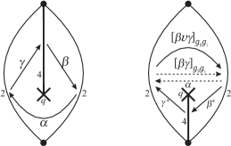
   Figure 25. Second configuration of Figure 23. Left: $\tau$ and $Q(\tau,\omega)$. Right: $\sigma$ and $\widetilde{\mu}_{k}(Q(\tau,\omega))$. The numbers next to the arcs are the corresponding values of the tuple $\mathbf{d}(\tau,\omega)$.

2. The SP $(A(\sigma,\zeta),S(\sigma,\zeta))$ is the reduced part of $(\widetilde{\mu}_{k}(A(\tau,\xi)),S(\sigma,\zeta)^{\sharp})$, where

   $$S(\sigma,\zeta)^{\sharp} = X\left(\alpha[\beta\gamma]_{g_{\beta}g_{\gamma}}+\gamma^{*}\beta^{*}[\beta v\gamma]_{g_{\beta}g_{\gamma}}\right)+S(\tau,\sigma)\in R\langle\langle\widetilde{\mu}_{k}(A(\tau,\xi))\rangle\rangle,$$

   with $S(\tau,\sigma)\in R\langle\langle A(\tau,\xi)\rangle\rangle\cap R\langle\langle A(\sigma,\zeta)\rangle\rangle$. Here, $X$ is an element of $\{0,1\}\subseteq F$ with the property of being equal to $1\in F$ (resp. $0\in F$) if and only if the two sides of the digon in Figure 25 are indeed arcs in $\tau$ (resp. at least one of the two sides of the digon is a boundary segment).

3. The potentials $S(\tau,\xi)$ and $\widetilde{\mu}_{k}(S(\tau,\xi))$ are

   $$S(\tau,\xi) = X\alpha\beta\gamma+S(\tau,\sigma)\ \ \ \ \ \text{and}$$

   $$\widetilde{\mu}_{k}(S(\tau,\xi)) \sim_{\operatorname{cyc}} X\left(\alpha[\beta\gamma]_{g_{\beta}g_{\gamma}}+\frac{1}{2}\left(\pi_{(g_{\beta}g_{\gamma})^{-1}}(\gamma^{*}\beta^{*})[\beta\gamma]_{g_{\beta}g_{\gamma}}+\gamma^{*}v^{-1}\beta^{*}[\beta v\gamma]_{g_{\beta}g_{\gamma}}\right)\right)+S(\tau,\sigma).$$

4. Since $\xi$ is a $1$-cocycle, from the definition of the modulating function $g$ it follows that $(g_{\beta}g_{\gamma})^{-1}=g_{\alpha}$, and hence the rule

   $$\varphi_{1} : X\alpha\mapsto X\left(\alpha-\frac{1}{2}\pi_{(g_{\beta}g_{\gamma})^{-1}}(\gamma^{*}\beta^{*})\right)$$

   yields a well-defined $R$-algebra automorphism $\varphi:R\langle\langle\widetilde{\mu}_{k}(A(\tau,\xi))\rangle\rangle\rightarrow R\langle\langle\widetilde{\mu}_{k}(A(\tau,\xi))\rangle\rangle$ (see [27, Propositions 2.15-(6) and 3.7]). Letting $\varphi_{2}:R\langle\langle\widetilde{\mu}_{k}(A(\tau,\xi))\rangle\rangle\rightarrow R\langle\langle\widetilde{\mu}_{k}(A(\tau,\xi))\rangle\rangle$ defined by the rule

   $$\varphi_{2} : X\beta^{*}\mapsto X2v\beta^{*},$$

   it is obvious that $\varphi_{2}\varphi_{1}$ is a right-equivalence $(\widetilde{\mu}_{k}(A(\tau,\xi)),\widetilde{\mu}_{k}(S(\tau,\xi)))\rightarrow(\widetilde{\mu}_{k}(A(\tau,\xi)),S(\sigma,\zeta)^{\sharp})$.

Case 3.

Configurations 3 and 7.

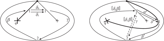
Figure 26. Configurations 3 and 7 of Figure 23. Left: $\tau$ and $Q(\tau,\omega)$. Right: $\sigma$ and $\widetilde{\mu}_{k}(Q(\tau,\omega))$. The numbers next to the arcs are the corresponding values of the tuple $\mathbf{d}(\tau,\omega)$.

1. We use the notation in Figure 26 and identify the quiver $Q(\sigma,\omega)$ with the subquiver of $\widetilde{\mu}_{k}(Q(\tau,\omega))$ obtained by deleting the dotted arrows in the quiver.

2. The SP $(A(\sigma,\zeta),S(\sigma,\zeta))$ is the reduced part of $(\widetilde{\mu}_{k}(A(\tau,\xi)),S(\sigma,\zeta)^{\sharp})$, where

   $$S(\sigma,\zeta)^{\sharp} = \gamma[\delta_{1}\beta]+u\beta^{*}\delta_{0}^{*}[\delta_{0}\beta]+\beta^{*}\delta_{1}^{*}[\delta_{0}\beta]+S(\tau,\sigma)\in R\langle\langle\widetilde{\mu}_{k}(A(\tau,\xi))\rangle\rangle,$$

   with $S(\tau,\sigma)\in R\langle\langle A(\tau,\xi)\rangle\rangle\cap R\langle\langle A(\sigma,\zeta)\rangle\rangle$.

3. The potentials $S(\tau,\xi)$ and $\widetilde{\mu}_{k}(S(\tau,\xi))$ are

   $$S(\tau,\xi) = \gamma\delta_{0}\beta+u\gamma\delta_{1}\beta+S(\tau,\sigma)\ \ \ \ \ \text{and}$$

   $$\widetilde{\mu}_{k}(S(\tau,\xi)) = \gamma[\delta_{0}\beta]+u\gamma[\delta_{1}\beta]+\beta^{*}\delta_{0}^{*}[\delta_{0}\beta]+\beta^{*}\delta_{1}^{*}[\delta_{1}\beta]+S(\tau,\sigma).$$

4. Define $R$-algebra automorphisms $\psi,\varphi,\Phi:R\langle\langle\widetilde{\mu}_{k}(A(\tau,\xi))\rangle\rangle\rightarrow R\langle\langle\widetilde{\mu}_{k}(A(\tau,\xi))\rangle\rangle$ according to the rules

   $$\psi : [\delta_{1}\beta]\mapsto[\delta_{1}\beta]u^{-1}-[\delta_{0}\beta]u^{-1}$$

   $$\varphi : \gamma\mapsto\gamma-u^{-1}\beta^{*}\delta_{1}^{*}$$

   $$\Phi : \delta_{1}^{*}\mapsto-\delta_{1}^{*},\ \ \ \ \ [\delta_{0}\beta]\mapsto[\delta_{0}\beta]u$$

   Direct computation shows that $\Phi\varphi\psi$ is a right-equivalence $(\widetilde{\mu}_{k}(A(\tau,\xi)),\widetilde{\mu}_{k}(S(\tau,\xi)))\rightarrow(\widetilde{\mu}_{k}(A(\tau,\xi)),S(\sigma,\zeta)^{\sharp})$.

Case 4.

Configuration 4 and 9.

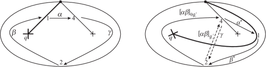
Figure 27. Configurations 4 and 9 of Figure 23. Left: $\tau$ and $Q(\tau,\omega)$. Right: $\sigma$ and $\widetilde{\mu}_{k}(Q(\tau,\omega))$. The numbers next to the arcs are the corresponding values of the tuple $\mathbf{d}(\tau,\omega)$.

1. We use the notation in Figure 27 and identify the quiver $Q(\sigma,\omega)$ with the subquiver of $\widetilde{\mu}_{k}(Q(\tau,\omega))$ obtained by deleting the dotted arrows in the figure.

2. The SP $(A(\sigma,\zeta),S(\sigma,\zeta))$ is the reduced part of $(\widetilde{\mu}_{k}(A(\tau,\xi)),S(\sigma,\zeta)^{\sharp})$, where

   $$S(\sigma,\zeta)^{\sharp} = \gamma[\alpha\beta]_{g_{\gamma}^{-1}}+\beta^{*}\alpha^{*}[\alpha\beta]_{\theta g_{\gamma}^{-1}}+S(\tau,\sigma)\in R\langle\langle\widetilde{\mu}_{k}(A(\tau,\xi))\rangle\rangle,$$

   with $S(\tau,\sigma)\in R\langle\langle A(\tau,\xi)\rangle\rangle\cap R\langle\langle A(\sigma,\zeta)\rangle\rangle$.

3. The potentials $S(\tau,\xi)$ and $\widetilde{\mu}_{k}(S(\tau,\xi))$ are

   $$S(\tau,\xi) = \gamma\alpha\beta+S(\tau,\sigma)\ \ \ \ \ \text{and}$$

   $$\widetilde{\mu}_{k}(S(\tau,\xi)) \sim_{\operatorname{cyc}} \gamma[\alpha\beta]_{g_{\gamma}^{-1}}+\pi_{g_{\gamma}}(\beta^{*}\alpha^{*})[\alpha\beta]_{g_{\gamma}^{-1}}+\beta^{*}\alpha^{*}[\alpha\beta]_{\theta g_{\gamma}^{-1}}+S(\tau,\sigma).$$

4. Define an $R$-algebra automorphism $\varphi:R\langle\langle\widetilde{\mu}_{k}(A(\tau,\xi))\rangle\rangle\rightarrow R\langle\langle\widetilde{\mu}_{k}(A(\tau,\xi))\rangle\rangle$ according to the rule

   $$\varphi : \gamma\mapsto\gamma-\pi_{g_{\gamma}}(\beta^{*}\alpha^{*})$$

   (that this rule indeed yields a well-defined $R$-algebra automorphism is a consequence of [27, Propositions 2.15-(6) and 3.7]). It is obvious that $\varphi$ is a right-equivalence $(\widetilde{\mu}_{k}(A(\tau,\xi)),\widetilde{\mu}_{k}(S(\tau,\xi)))\rightarrow(\widetilde{\mu}_{k}(A(\tau,\xi)),S(\sigma,\zeta)^{\sharp})$.

Case 5.

Configurations 5 and 8.

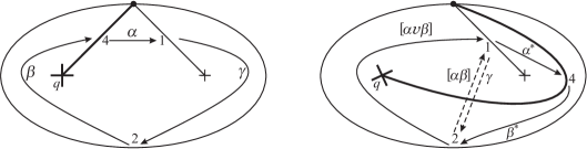
Figure 28. Configurations 5 and 8 of Figure 23. Left: $\tau$ and $Q(\tau,\omega)$. Right: $\sigma$ and $\widetilde{\mu}_{k}(Q(\tau,\omega))$. The numbers next to the arcs are the corresponding values of the tuple $\mathbf{d}(\tau,\omega)$.

1. We use the notation in Figure 28 and identify the quiver $Q(\sigma,\omega)$ with the subquiver of $\widetilde{\mu}_{k}(Q(\tau,\omega))$ obtained by deleting the dotted arrows in the figure.

2. The SP $(A(\sigma,\zeta),S(\sigma,\zeta))$ is the reduced part of $(\widetilde{\mu}_{k}(A(\tau,\xi)),S(\sigma,\zeta)^{\sharp})$, where

   $$S(\sigma,\zeta)^{\sharp} = \gamma[\alpha\beta]+\beta^{*}\alpha^{*}[\alpha v\beta]+S(\tau,\sigma)\in R\langle\langle\widetilde{\mu}_{k}(A(\tau,\xi))\rangle\rangle,$$

   with $S(\tau,\sigma)\in R\langle\langle A(\tau,\xi)\rangle\rangle\cap R\langle\langle A(\sigma,\zeta)\rangle\rangle$.

3. The potentials $S(\tau,\xi)$ and $\widetilde{\mu}_{k}(S(\tau,\xi))$ are

   $$S(\tau,\xi) = \gamma\alpha\beta+S(\tau,\sigma)\ \ \ \ \ \text{and}$$

   $$\widetilde{\mu}_{k}(S(\tau,\xi)) = \gamma[\alpha\beta]+\frac{1}{2}\left(\beta^{*}\alpha^{*}[\alpha\beta]+\beta^{*}v^{-1}\alpha^{*}[\alpha v\beta]\right)+S(\tau,\sigma).$$

4. Define $R$-algebra automorphisms $\varphi,\Phi:R\langle\langle\widetilde{\mu}_{k}(A(\tau,\xi))\rangle\rangle\rightarrow R\langle\langle\widetilde{\mu}_{k}(A(\tau,\xi))\rangle\rangle$ according to the rules

   $\varphi$

   :

   $\gamma\mapsto\gamma-\frac{1}{2}\beta^{*}\alpha^{*}$,

   $\Phi$

   :

   $\alpha^{*}\mapsto 2v\alpha^{*}$.

   An easy computation shows that $\Phi\varphi$ is a right-equivalence $(\widetilde{\mu}_{k}(A(\tau,\xi)),\widetilde{\mu}_{k}(S(\tau,\xi)))\rightarrow(\widetilde{\mu}_{k}(A(\tau,\xi)),S(\sigma,\zeta)^{\sharp})$.

Case 6.

Configurations 6 and 10.

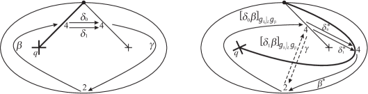
Figure 29. Configurations 6 and 10 of Figure 23. Left: $\tau$ and $Q(\tau,\omega)$. Right: $\sigma$ and $\widetilde{\mu}_{k}(Q(\tau,\omega))$. The numbers next to the arcs are the corresponding values of the tuple $\mathbf{d}(\tau,\omega)$.

1. We use the notation in Figure 29 and identify the quiver $Q(\sigma,\omega)$ with the subquiver of $\widetilde{\mu}_{k}(Q(\tau,\omega))$ obtained by deleting the dotted arrows in the figure.

2. The SP $(A(\sigma,\zeta),S(\sigma,\zeta))$ is the reduced part of $(\widetilde{\mu}_{k}(A(\tau,\xi)),S(\sigma,\zeta)^{\sharp})$, where

   $$S(\sigma,\zeta)^{\sharp} = \gamma[\delta_{1}\beta]_{g_{\delta_{1}}|_{L}g_{\beta}}+\beta^{*}(\delta_{0}^{*}+\delta_{1}^{*})[\delta_{0}\beta]_{g_{\delta_{0}}|_{L}g_{\beta}}+S(\tau,\sigma)\in R\langle\langle\widetilde{\mu}_{k}(A(\tau,\xi))\rangle\rangle,$$

   with $S(\tau,\sigma)\in R\langle\langle A(\tau,\xi)\rangle\rangle\cap R\langle\langle A(\sigma,\zeta)\rangle\rangle$.

3. The potentials $S(\tau,\xi)$ and $\widetilde{\mu}_{k}(S(\tau,\xi))$ are

   $$S(\tau,\xi) = (\delta_{0}+\delta_{1})\beta\gamma+S(\tau,\sigma)\ \ \ \ \ \text{and}$$

   $$\widetilde{\mu}_{k}(S(\tau,\xi)) \sim_{\operatorname{cyc}} \gamma[\delta_{0}\beta]_{g_{\delta_{0}}|_{L}g_{\beta}}+\gamma[\delta_{1}\beta]_{g_{\delta_{1}}|_{L}g_{\beta}}$$

   $$+\beta^{*}\delta_{0}^{*}[\delta_{0}\beta]_{g_{\delta_{0}}|_{L}g_{\beta}}+\pi_{(g_{\delta_{1}}|_{L}g_{\beta})^{-1}}(\beta^{*}\delta_{1}^{*})[\delta_{1}\beta]_{g_{\delta_{1}}|_{L}g_{\beta}}+S(\tau,\sigma).$$

4. Since $\xi$ is a $1$-cocycle, from the definition of the modulating function $g$ it follows that $g_{\delta_{0}}|_{L}g_{\beta}=g_{\delta_{1}}|_{L}g_{\beta}=g_{\gamma}^{-1}$, from which we deduce that the rules

   $$\psi : [\delta_{1}\beta]_{g_{\delta_{1}}|_{L}g_{\beta}}\mapsto[\delta_{1}\beta]_{g_{\delta_{1}}|_{L}g_{\beta}}-[\delta_{0}\beta]_{g_{\delta_{0}}|_{L}g_{\beta}|_{L}}$$

   $$\varphi : \gamma\mapsto\gamma-\pi_{(g_{\delta_{1}}|_{L}g_{\beta})^{-1}}(\beta^{*}\delta_{1}^{*})$$

   produce well-defined $R$-algebra automorphisms $\psi,\varphi:R\langle\langle\widetilde{\mu}_{k}(A(\tau,\xi))\rangle\rangle\rightarrow R\langle\langle\widetilde{\mu}_{k}(A(\tau,\xi))\rangle\rangle$ (see [27, Propositions 2.15-(6) and 3.7]). Letting $\Phi:R\langle\langle\widetilde{\mu}_{k}(A(\tau,\xi))\rangle\rangle\rightarrow R\langle\langle\widetilde{\mu}_{k}(A(\tau,\xi))\rangle\rangle$ be the $R$-algebra automorphism defined by the rule

   $$\Phi : \delta_{1}^{*}\mapsto-\delta_{1}^{*},$$

   direct computation shows that $\Phi\varphi\psi$ is a right-equivalence $(\widetilde{\mu}_{k}(A(\tau,\xi)),\widetilde{\mu}_{k}(S(\tau,\xi)))\rightarrow(\widetilde{\mu}_{k}(A(\tau,\xi)),S(\sigma,\zeta)^{\sharp})$.

Case 7.

Configuration 11.

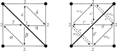
Figure 30. Configuration 11 of Figure 23. Left: $\tau$ and $Q(\tau,\omega)$. Right: $\sigma$ and $\widetilde{\mu}_{k}(Q(\tau,\omega))$. The numbers next to the arcs are the corresponding values of the tuple $\mathbf{d}(\tau,\omega)$.

1. We use the notation in Figure 30 and identify the quiver $Q(\sigma,\omega)$ with the subquiver of $\widetilde{\mu}_{k}(Q(\tau,\omega))$ obtained by deleting the dotted arrows in the figure.

2. The SP $(A(\sigma,\zeta),S(\sigma,\zeta))$ is the reduced part of $(\widetilde{\mu}_{k}(A(\tau,\xi)),S(\sigma,\zeta)^{\sharp})$, where

   $$S(\sigma,\zeta)^{\sharp} = \alpha[\beta\gamma]_{g_{\beta}g_{\gamma}}+\delta[\varepsilon\eta]_{g_{\varepsilon}g_{\eta}}+\gamma^{*}\varepsilon^{*}[\varepsilon\gamma]_{g_{\varepsilon}g_{\gamma}}+\eta^{*}\beta^{*}[\beta\eta]_{g_{\beta}g_{\eta}}+S(\tau,\sigma)\in R\langle\langle\widetilde{\mu}_{k}(A(\tau,\xi))\rangle\rangle,$$

   with $S(\tau,\sigma)\in R\langle\langle A(\tau,\xi)\rangle\rangle\cap R\langle\langle A(\sigma,\zeta)\rangle\rangle$.

3. The potentials $S(\tau,\xi)$ and $\widetilde{\mu}_{k}(S(\tau,\xi))$ are

   $$S(\tau,\xi) = \alpha\beta\gamma+\delta\varepsilon\eta+S(\tau,\sigma)\ \ \ \ \ \text{and}$$

   $$\widetilde{\mu}_{k}(S(\tau,\xi)) \sim_{\operatorname{cyc}} \alpha[\beta\gamma]_{g_{\beta}g_{\gamma}}+\delta[\varepsilon\eta]_{g_{\varepsilon}g_{\eta}}$$

   $$+\pi_{(g_{\beta}g_{\gamma})^{-1}}(\gamma^{*}\beta^{*})[\beta\gamma]_{{}_{\beta}g_{\gamma}}+\pi_{(g_{\varepsilon}g_{\eta})^{-1}}(\eta^{*}\varepsilon^{*})[\varepsilon\eta]_{g_{\varepsilon}g_{\eta}}$$

   $$+\gamma^{*}\varepsilon^{*}[\varepsilon\gamma]_{g_{\varepsilon}g_{\gamma}}+\eta^{*}\beta^{*}[\beta\eta]_{g_{\beta}g_{\eta}}+S(\tau,\sigma).$$

4. Since $\xi$ is a $1$-cocycle, from the definition of the modulating function $g$ it follows that $g_{\beta}g_{\gamma}=g_{\alpha}^{-1}$ and $g_{\varepsilon}g_{\eta}=g_{\delta}^{-1}$, from which we deduce that the rule

   $\varphi$

   :

   $\alpha\mapsto\alpha-\pi_{(g_{\beta}g_{\gamma})^{-1}}(\gamma^{*}\beta^{*})$,

   $\delta\mapsto\delta-\pi_{(g_{\varepsilon}g_{\eta})^{-1}}(\eta^{*}\varepsilon^{*})$,

   produces a well-defined $R$-algebra automorphisms $\varphi:R\langle\langle\widetilde{\mu}_{k}(A(\tau,\xi))\rangle\rangle\rightarrow R\langle\langle\widetilde{\mu}_{k}(A(\tau,\xi))\rangle\rangle$ (see [27, Propositions 2.15-(6) and 3.7]). It is obvious that $\varphi$ is a right-equivalence $(\widetilde{\mu}_{k}(A(\tau,\xi)),\widetilde{\mu}_{k}(S(\tau,\xi)))\rightarrow(\widetilde{\mu}_{k}(A(\tau,\xi)),S(\sigma,\zeta)^{\sharp})$.

Case 8.

Configurations 12 and 14.

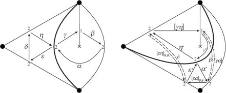
Figure 31. Configurations 12 and 14 of Figure 23. Left: $\tau$ and $Q(\tau,\omega)$. Right: $\sigma$ and $\widetilde{\mu}_{k}(Q(\tau,\omega))$. The numbers next to the arcs are the corresponding values of the tuple $\mathbf{d}(\tau,\omega)$.

1. We use the notation in Figure 31 and identify the quiver $Q(\sigma,\omega)$ with the subquiver of $\widetilde{\mu}_{k}(Q(\tau,\omega))$ obtained by deleting the dotted arrows in the figure.

2. The SP $(A(\sigma,\zeta),S(\sigma,\zeta))$ is the reduced part of $(\widetilde{\mu}_{k}(A(\tau,\xi)),S(\sigma,\zeta)^{\sharp})$, where

   $$S(\sigma,\zeta)^{\sharp} = \beta[\gamma\alpha]+\delta[\varepsilon\eta]_{g_{\varepsilon}g_{\eta}}+\alpha^{*}\varepsilon^{*}[\varepsilon\alpha]_{g_{\varepsilon}g_{\alpha}}+\eta^{*}\gamma^{*}[\gamma\eta]+S(\tau,\sigma)\in R\langle\langle\widetilde{\mu}_{k}(A(\tau,\xi))\rangle\rangle,$$

   with $S(\tau,\sigma)\in R\langle\langle A(\tau,\xi)\rangle\rangle\cap R\langle\langle A(\sigma,\zeta)\rangle\rangle$.

3. The potentials $S(\tau,\xi)$ and $\widetilde{\mu}_{k}(S(\tau,\xi))$ are

   $$S(\tau,\xi) = \alpha\beta\gamma+\varepsilon\eta\delta+S(\tau,\sigma)\ \ \ \ \ \text{and}$$

   $$\widetilde{\mu}_{k}(S(\tau,\xi)) \sim_{\operatorname{cyc}} \beta[\gamma\alpha]+\delta[\varepsilon\eta]_{g_{\varepsilon}g_{\eta}}$$

   $$+\alpha^{*}\gamma^{*}[\gamma\alpha]+\pi_{(g_{\varepsilon}g_{\eta})^{-1}}(\eta^{*}\varepsilon^{*})[\varepsilon\eta]_{g_{\varepsilon}g_{\eta}}+\alpha^{*}\varepsilon^{*}[\varepsilon\alpha]_{g_{\varepsilon}g_{\alpha}}+\eta^{*}\gamma^{*}[\gamma\eta]+S(\tau,\sigma).$$

4. Since $\xi$ is a $1$-cocycle, from the definition of the modulating function $g$ it follows that $g_{\varepsilon}g_{\eta}=g_{\delta}^{-1}$, from which we deduce that the rule

   $\varphi$

   :

   $\beta\mapsto\beta-\alpha^{*}\gamma^{*}$,

   $\delta\mapsto\delta-\pi_{(g_{\varepsilon}g_{\eta})^{-1}}(\eta^{*}\varepsilon^{*})$,

   produces a well-defined $R$-algebra automorphism $\varphi:R\langle\langle\widetilde{\mu}_{k}(A(\tau,\xi))\rangle\rangle\rightarrow R\langle\langle\widetilde{\mu}_{k}(A(\tau,\xi))\rangle\rangle$ (see [27, Propositions 2.15-(6) and 3.7]). It is obvious that $\varphi$ is a right-equivalence $(\widetilde{\mu}_{k}(A(\tau,\xi)),\widetilde{\mu}_{k}(S(\tau,\xi)))\rightarrow(\widetilde{\mu}_{k}(A(\tau,\xi)),S(\sigma,\zeta)^{\sharp})$.

Case 9.

Configurations 13 and 15.

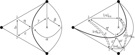
Figure 32. Configurations 13 and 15 of Figure 23. Left: $\tau$ and $Q(\tau,\omega)$. Right: $\sigma$ and $\widetilde{\mu}_{k}(Q(\tau,\omega))$. The numbers next to the arcs are the corresponding values of the tuple $\mathbf{d}(\tau,\omega)$.

1. We use the notation in Figure 32 and identify the quiver $Q(\sigma,\omega)$ with the subquiver of $\widetilde{\mu}_{k}(Q(\tau,\omega))$ obtained by deleting the dotted arrows in the figure.

2. The SP $(A(\sigma,\zeta),S(\sigma,\zeta))$ is the reduced part of $(\widetilde{\mu}_{k}(A(\tau,\xi)),S(\sigma,\zeta)^{\sharp})$, where

   $$S(\sigma,\zeta)^{\sharp} = \delta[\varepsilon\eta]_{g_{\varepsilon}g_{\eta}}+\beta[\gamma\alpha]_{g_{\gamma}g_{\alpha}}+\eta^{*}\gamma^{*}[\gamma\eta]_{g_{\gamma}g_{\eta}}+\alpha^{*}\varepsilon^{*}[\varepsilon\alpha]_{g_{\varepsilon}g_{\alpha}}+S(\tau,\sigma)\in R\langle\langle\widetilde{\mu}_{k}(A(\tau,\xi))\rangle\rangle,$$

   with $S(\tau,\sigma)\in R\langle\langle A(\tau,\xi)\rangle\rangle\cap R\langle\langle A(\sigma,\zeta)\rangle\rangle$.

3. The potentials $S(\tau,\xi)$ and $\widetilde{\mu}_{k}(S(\tau,\xi))$ are

   $$S(\tau,\xi) = \delta\varepsilon\eta+\beta\gamma\alpha+S(\tau,\sigma)\ \ \ \ \ \text{and}$$

   $$\widetilde{\mu}_{k}(S(\tau,\xi)) \sim_{\operatorname{cyc}} \delta[\varepsilon\eta]_{g_{\varepsilon}g_{\eta}}+\beta[\gamma\alpha]_{g_{\gamma}g_{\alpha}}$$

   $$+\pi_{(g_{\varepsilon}g_{\eta})^{-1}}(\eta^{*}\varepsilon^{*})[\varepsilon\eta]_{g_{\varepsilon}g_{\eta}}+\pi_{(g_{\gamma}g_{\alpha})^{-1}}(\alpha^{*}\gamma^{*})[\gamma\alpha]_{g_{\gamma}g_{\alpha}}$$

   $$+\eta^{*}\gamma^{*}[\gamma\eta]_{g_{\gamma}g_{\eta}}+\alpha^{*}\varepsilon^{*}[\varepsilon\alpha]_{g_{\varepsilon}g_{\alpha}}+S(\tau,\sigma).$$

4. Since $\xi$ is a $1$-cocycle, from the definition of the modulating function $g$ it follows that $g_{\varepsilon}g_{\eta}=g_{\delta}^{-1}$ and $g_{\gamma}g_{\alpha}=g_{\beta}^{-1}$, from which we deduce that the rule

   $\varphi$

   :

   $\delta\mapsto\delta-\pi_{(g_{\varepsilon}g_{\eta})^{-1}}(\eta^{*}\varepsilon^{*})$,

   $\beta\mapsto\beta-\pi_{(g_{\gamma}g_{\alpha})^{-1}}(\alpha^{*}\gamma^{*})$,

   produces a well-defined $R$-algebra automorphism $\varphi:R\langle\langle\widetilde{\mu}_{k}(A(\tau,\xi))\rangle\rangle\rightarrow R\langle\langle\widetilde{\mu}_{k}(A(\tau,\xi))\rangle\rangle$ (see [27, Propositions 2.15-(6) and 3.7]). It is obvious that $\varphi$ is a right-equivalence $(\widetilde{\mu}_{k}(A(\tau,\xi)),\widetilde{\mu}_{k}(S(\tau,\xi)))\rightarrow(\widetilde{\mu}_{k}(A(\tau,\xi)),S(\sigma,\zeta)^{\sharp})$.

Case 10.

Configurations 20 and 16.

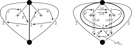
Figure 33. Configurations 20 and 16 of Figure 23. Left: $\tau$ and $Q(\tau,\omega)$. Right: $\sigma$ and $\widetilde{\mu}_{k}(Q(\tau,\omega))$. The numbers next to the arcs are the corresponding values of the tuple $\mathbf{d}(\tau,\omega)$.

1. We use the notation in Figure 33 and identify the quiver $Q(\sigma,\omega)$ with the subquiver of $\widetilde{\mu}_{k}(Q(\tau,\omega))$ obtained by deleting the dotted arrows in the figure.

2. The SP $(A(\sigma,\zeta),S(\sigma,\zeta))$ is the reduced part of $(\widetilde{\mu}_{k}(A(\tau,\xi)),S(\sigma,\zeta)^{\sharp})$, where

   $$S(\sigma,\zeta)^{\sharp} = \gamma[\alpha\beta]+\eta[\varepsilon\delta]+\delta^{*}\alpha^{*}[\alpha\delta]_{g_{\alpha}g_{\delta}}+[\varepsilon\beta]\beta^{*}u\varepsilon^{*}+[\varepsilon u\beta]\beta^{*}\varepsilon^{*}+S(\tau,\sigma)\in R\langle\langle\widetilde{\mu}_{k}(A(\tau,\xi))\rangle\rangle,$$

   with $S(\tau,\sigma)\in R\langle\langle A(\tau,\xi)\rangle\rangle\cap R\langle\langle A(\sigma,\zeta)\rangle\rangle$.

3. The potentials $S(\tau,\xi)$ and $\widetilde{\mu}_{k}(S(\tau,\xi))$ are

   $$S(\tau,\xi) = \alpha\beta\gamma+\delta\eta\varepsilon+S(\tau,\sigma),\ \ \ \ \ \text{and}$$

   $$\widetilde{\mu}_{k}(S(\tau,\xi)) = \gamma[\alpha\beta]+\eta[\varepsilon\delta]+\beta^{*}\alpha^{*}[\alpha\beta]+\delta^{*}\varepsilon^{*}[\varepsilon\delta]+\beta^{*}\varepsilon^{*}[\varepsilon\beta]+\beta^{*}u^{-1}\varepsilon^{*}[\varepsilon u\beta]+\delta^{*}\alpha^{*}[\alpha\delta]_{g_{\alpha}g_{\delta}}+S(\tau,\sigma).$$

4. From the definition of the modulating function $g$ it obviously follows that $g_{\alpha}g_{\beta}=g_{\gamma}^{-1}$, $g_{\varepsilon}g_{\delta}=g_{\eta}^{-1}$, $\pi_{(g_{\alpha}g_{\beta})^{-1}}(\beta^{*}\alpha^{*})=\beta^{*}\alpha^{*}$ and $\pi_{(g_{\varepsilon}g_{\delta})^{-1}(\delta^{*}\varepsilon^{*})}=\delta^{*}\varepsilon^{*}$, from which we deduce that the rule

   $\varphi$

   :

   $\gamma\mapsto\gamma-\beta^{*}\alpha^{*}$,

   $\eta\mapsto\eta-\delta^{*}\varepsilon^{*}$

   produces a well-defined $R$-algebra automorphism $\varphi:R\langle\langle\widetilde{\mu}_{k}(A(\tau,\xi))\rangle\rangle\rightarrow R\langle\langle\widetilde{\mu}_{k}(A(\tau,\xi))\rangle\rangle$ (see [27, Propositions 2.15-(6) and 3.7]). Letting $\Phi:R\langle\langle\widetilde{\mu}_{k}(A(\tau,\xi))\rangle\rangle\rightarrow R\langle\langle\widetilde{\mu}_{k}(A(\tau,\xi))\rangle\rangle$ be the $R$-algebra automorphism defined by the rule

   $$\Phi : \varepsilon^{*}\mapsto u\varepsilon^{*},$$

   direct computation shows that $\Phi\varphi$ is a right-equivalence $(\widetilde{\mu}_{k}(A(\tau,\xi)),\widetilde{\mu}_{k}(S(\tau,\xi)))\rightarrow(\widetilde{\mu}_{k}(A(\tau,\xi)),S(\sigma,\zeta)^{\sharp})$.

Case 11.

Configurations 21 and 17.

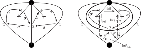
Figure 34. Configurations 21 and 17 of Figure 23. Left: $\tau$ and $Q(\tau,\omega)$. Right: $\sigma$ and $\widetilde{\mu}_{k}(Q(\tau,\omega))$. The numbers next to the arcs are the corresponding values of the tuple $\mathbf{d}(\tau,\omega)$.

1. We use the notation in Figure 34 and identify the quiver $Q(\sigma,\omega)$ with the subquiver of $\widetilde{\mu}_{k}(Q(\tau,\omega))$ obtained by deleting the dotted arrows in the figure.

2. The SP $(A(\sigma,\zeta),S(\sigma,\zeta))$ is the reduced part of $(\widetilde{\mu}_{k}(A(\tau,\xi)),S(\sigma,\zeta)^{\sharp})$, where

   $$S(\sigma,\zeta)^{\sharp} = \gamma[\alpha\beta]+\eta[\varepsilon\delta]_{g_{\varepsilon}g_{\delta}}+\delta^{*}\alpha^{*}[\alpha\delta]_{g_{\alpha}g_{\delta}}+[\varepsilon\beta]\beta^{*}\varepsilon^{*}+S(\tau,\sigma)\in R\langle\langle\widetilde{\mu}_{k}(A(\tau,\xi))\rangle\rangle,$$

   with $S(\tau,\sigma)\in R\langle\langle A(\tau,\xi)\rangle\rangle\cap R\langle\langle A(\sigma,\zeta)\rangle\rangle$. Furthermore,

   $$S(\tau,\xi) = \alpha\beta\gamma+\delta\eta\varepsilon+S(\tau,\sigma)\ \ \ \ \ \text{and}$$

   $$\widetilde{\mu}_{k}(S(\tau,\xi)) \sim_{\operatorname{cyc}} \gamma[\alpha\beta]+\eta[\varepsilon\delta]_{g_{\varepsilon}g_{\delta}}+\beta^{*}\alpha^{*}[\alpha\beta]+\pi_{(g_{\varepsilon}g_{\delta})^{-1}}(\delta^{*}\varepsilon^{*})[\varepsilon\delta]_{g_{\varepsilon}g_{\delta}}$$

   $$+\beta^{*}\varepsilon^{*}[\varepsilon\beta]+\delta^{*}\alpha^{*}[\alpha\delta]_{g_{\alpha}g_{\delta}}+S(\tau,\sigma).$$

3. From the equalities $g_{\varepsilon}g_{\delta}=g_{\eta}^{-1}$, $g_{\alpha}g_{\beta}=g_{\gamma}^{-1}$ and $\pi_{(g_{\alpha}g_{\beta})^{-1}}(\beta^{*}\alpha^{*})=\beta^{*}\alpha^{*}$, we deduce that the rule

   $\varphi$

   :

   $\gamma\mapsto\gamma-\beta^{*}\alpha^{*}$,

   $\eta\mapsto\eta-\pi_{(g_{\varepsilon}g_{\delta})^{-1}}(\delta^{*}\varepsilon^{*})$,

   produces a well-defined $R$-algebra automorphism $\varphi:R\langle\langle\widetilde{\mu}_{k}(A(\tau,\xi))\rangle\rangle\rightarrow R\langle\langle\widetilde{\mu}_{k}(A(\tau,\xi))\rangle\rangle$ (see [27, Propositions 2.15-(6) and 3.7]). It turns out to be obvious that $\varphi$ is a right-equivalence $(\widetilde{\mu}_{k}(A(\tau,\xi)),\widetilde{\mu}_{k}(S(\tau,\xi)))\rightarrow(\widetilde{\mu}_{k}(A(\tau,\xi)),S(\sigma,\zeta)^{\sharp})$.

Case 12.

Configurations 22 and 18.

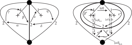
Figure 35. Configurations 22 and 18 of Figure 23. Left: $\tau$ and $Q(\tau,\omega)$. Right: $\sigma$ and $\widetilde{\mu}_{k}(Q(\tau,\omega))$ appear on the right. The numbers next to the arcs are the corresponding values of the tuple $\mathbf{d}(\tau,\omega)$.

1. We use the notation in Figure 35 and identify the quiver $Q(\sigma,\omega)$ with the subquiver of $\widetilde{\mu}_{k}(Q(\tau,\omega))$ obtained by deleting the dotted arrows in the figure.

2. The SP $(A(\sigma,\zeta),S(\sigma,\zeta))$ is the reduced part of $(\widetilde{\mu}_{k}(A(\tau,\xi)),S(\sigma,\zeta)^{\sharp})$, where

   $$S(\sigma,\zeta)^{\sharp} = \gamma[\alpha\beta]_{g_{\alpha}g_{\beta}}+\eta[\varepsilon\delta]+\delta^{*}\alpha^{*}[\alpha\delta]_{g_{\alpha}g_{\delta}}+[\varepsilon\beta]\beta^{*}\varepsilon^{*}+S(\tau,\sigma)\in R\langle\langle\widetilde{\mu}_{k}(A(\tau,\xi))\rangle\rangle,$$

   with $S(\tau,\sigma)\in R\langle\langle A(\tau,\xi)\rangle\rangle\cap R\langle\langle A(\sigma,\zeta)\rangle\rangle$.

3. The potentials $S(\tau,\xi)$ and $\widetilde{\mu}_{k}(S(\tau,\xi))$ are

   $$S(\tau,\xi) = \alpha\beta\gamma+\delta\eta\varepsilon+S(\tau,\sigma)\ \ \ \ \ \text{and}$$

   $$\widetilde{\mu}_{k}(S(\tau,\xi)) \sim_{\operatorname{cyc}} \gamma[\alpha\beta]_{g_{\alpha}g_{\beta}}+\eta[\varepsilon\delta]+\pi_{(g_{\alpha}g_{\beta})^{-1}}(\beta^{*}\alpha^{*})[\alpha\beta]_{g_{\alpha}g_{\beta}}+\delta^{*}\varepsilon^{*}[\varepsilon\delta]$$

   $$+\beta^{*}\varepsilon^{*}[\varepsilon\beta]+\delta^{*}\alpha^{*}[\alpha\delta]_{g_{\alpha}g_{\delta}}+S(\tau,\sigma).$$

4. From the equalities $g_{\alpha}g_{\beta}=g_{\gamma}^{-1}$, $g_{\varepsilon}g_{\delta}=g_{\eta}^{-1}$ and $\pi_{(g_{\varepsilon}g_{\delta})^{-1}}(\delta^{*}\varepsilon^{*})=\delta^{*}\varepsilon^{*}$, we deduce that the rule

   $\varphi$

   :

   $\gamma\mapsto\gamma-\pi_{(g_{\alpha}g_{\beta})^{-1}}(\beta^{*}\alpha^{*})$,

   $\eta\mapsto\eta-\delta^{*}\varepsilon^{*}$,

   produces a well-defined $R$-algebra automorphism $\varphi:R\langle\langle\widetilde{\mu}_{k}(A(\tau,\xi))\rangle\rangle\rightarrow R\langle\langle\widetilde{\mu}_{k}(A(\tau,\xi))\rangle\rangle$ (see [27, Propositions 2.15-(6) and 3.7]). It turns out to be obvious that $\varphi$ is a right-equivalence $(\widetilde{\mu}_{k}(A(\tau,\xi)),\widetilde{\mu}_{k}(S(\tau,\xi)))\rightarrow(\widetilde{\mu}_{k}(A(\tau,\xi)),S(\sigma,\zeta)^{\sharp})$.

Case 13.

Configurations 23 and 19.

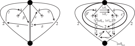
Figure 36. Configurations 23 and 19 of Figure 23. Left: $\tau$ and $Q(\tau,\omega)$. Right: $\sigma$ and $\widetilde{\mu}_{k}(Q(\tau,\omega))$. The numbers next to the arcs are the corresponding values of the tuple $\mathbf{d}(\tau,\omega)$.

1. We use the notation in Figure 36, where the element $j\in\{0,1,2,3\}$ satisfies $\rho^{j}|_{L}=g_{\varepsilon}g_{\beta}=\rho^{j+2}|_{L}$ and identify the quiver $Q(\sigma,\omega)$ with the subquiver of $\widetilde{\mu}_{k}(Q(\tau,\omega))$ obtained by deleting the dotted arrows in the figure. By the definition of the modulating function $\widetilde{\mu}_{k}(g):\widetilde{\mu}_{k}(Q(\tau,\xi))_{1}\rightarrow\bigcup_{i,j\in\tau}G_{i,j}$ (cf. [27, Definition 3.19]), we have

   $\widetilde{\mu}_{k}(g)([\alpha\delta]_{g_{\alpha}g_{\delta}})=g_{\alpha}g_{\delta}$,

   $\widetilde{\mu}_{k}(g)([\varepsilon\beta]_{\rho^{j}})=\rho^{j}$

   and

   $\widetilde{\mu}_{k}(g)([\varepsilon\beta]_{\rho^{j+2}})=\rho^{j+2}$,

   which respectively coincide with $\theta^{\zeta([\alpha\delta]_{g_{\alpha}g_{\delta}})}$, $g(\sigma,\zeta)_{[\varepsilon\beta]_{\rho^{j}}}$ and $g(\sigma,\zeta)_{[\varepsilon\beta]_{\rho^{j+2}}}$ since $(\sigma,\zeta)=f_{k}(\tau,\xi)$.

2. The SP $(A(\sigma,\zeta),S(\sigma,\zeta))$ is the reduced part of $(\widetilde{\mu}_{k}(A(\tau,\xi)),S(\sigma,\zeta)^{\sharp})$, where

   $$S(\sigma,\zeta)^{\sharp} = \gamma[\alpha\beta]_{g_{\alpha}g_{\beta}}+\eta[\varepsilon\delta]_{g_{\varepsilon}g_{\delta}}+\delta^{*}\alpha^{*}[\alpha\delta]_{g_{\alpha}g_{\delta}}+([\varepsilon\beta]_{\rho^{j}}+[\varepsilon\beta]_{\rho^{j+2}})\beta^{*}\varepsilon^{*}+S(\tau,\sigma)\in R\langle\langle\widetilde{\mu}_{k}(A(\tau,\xi))\rangle\rangle,$$

   with $S(\tau,\sigma)\in R\langle\langle A(\tau,\xi)\rangle\rangle\cap R\langle\langle A(\sigma,\zeta)\rangle\rangle$. Furthermore,

   $$S(\tau,\xi) = \alpha\beta\gamma+\delta\eta\varepsilon+S(\tau,\sigma)\ \ \ \ \ \text{and}$$

   $$\widetilde{\mu}_{k}(S(\tau,\xi)) \sim_{\operatorname{cyc}} \gamma[\alpha\beta]_{g_{\alpha}g_{\beta}}+\eta[\varepsilon\delta]_{g_{\varepsilon}g_{\delta}}$$

   $$+\pi_{(g_{\alpha}g_{\beta})^{-1}}(\beta^{*}\alpha^{*})[\alpha\beta]_{g_{\alpha}g_{\beta}}+\pi_{(g_{\varepsilon}g_{\delta})^{-1}}(\delta^{*}\varepsilon^{*})[\varepsilon\delta]_{g_{\varepsilon}g_{\delta}}$$

   $$+\beta^{*}\varepsilon^{*}([\varepsilon\beta]_{\rho^{j}}+[\varepsilon\beta]_{\rho^{j+2}})+\delta^{*}\alpha^{*}[\alpha\delta]_{g_{\alpha}g_{\delta}}+S(\tau,\sigma).$$

3. From the equalities $g_{\alpha}g_{\beta}=g_{\gamma}^{-1}$ and $g_{\varepsilon}g_{\delta}=g_{\eta}^{-1}$, we deduce that the rule

   $\varphi$

   :

   $\gamma\mapsto\gamma-\pi_{(g_{\alpha}g_{\beta})^{-1}}(\beta^{*}\alpha^{*})$,

   $\eta\mapsto\eta-\pi_{(g_{\varepsilon}g_{\delta})^{-1}}(\delta^{*}\varepsilon^{*})$,

   produces a well-defined $R$-algebra automorphism $\varphi:R\langle\langle\widetilde{\mu}_{k}(A(\tau,\xi))\rangle\rangle\rightarrow R\langle\langle\widetilde{\mu}_{k}(A(\tau,\xi))\rangle\rangle$ (see [27, Propositions 2.15-(6) and 3.7]). It turns out to be obvious that $\varphi$ is a right-equivalence $(\widetilde{\mu}_{k}(A(\tau,\xi)),\widetilde{\mu}_{k}(S(\tau,\xi)))\rightarrow(\widetilde{\mu}_{k}(A(\tau,\xi)),S(\sigma,\zeta)^{\sharp})$.

Case 14.

Configurations 24 and 28.

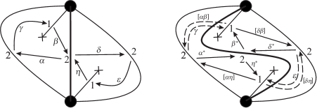
Figure 37. Configurations 24 and 28 of Figure 23. Left: $\tau$ and $Q(\tau,\omega)$. Right: $\sigma$ and $\widetilde{\mu}_{k}(Q(\tau,\omega))$. The numbers next to the arcs are the corresponding values of the tuple $\mathbf{d}(\tau,\omega)$.

1. We use the notation in Figure 37 and identify the quiver $Q(\sigma,\omega)$ with the subquiver of $\widetilde{\mu}_{k}(Q(\tau,\omega))$ obtained by deleting the dotted arrows in the figure.

2. It is straightforward to see that $(A(\sigma,\zeta),S(\sigma,\zeta))$ is the reduced part of $(\widetilde{\mu}_{k}(A(\tau,\xi)),S(\sigma,\zeta)^{\sharp})$, where

   $$S(\sigma,\zeta)^{\sharp} = \gamma[\alpha\beta]+\varepsilon[\delta\eta]+\eta^{*}\alpha^{*}[\alpha\eta]+\beta^{*}\delta^{*}[\delta\beta]+S(\tau,\sigma)\in R\langle\langle\widetilde{\mu}_{k}(A(\tau,\xi))\rangle\rangle,$$

   with $S(\tau,\sigma)\in R\langle\langle A(\tau,\xi)\rangle\rangle\cap R\langle\langle A(\sigma,\zeta)\rangle\rangle$.

3. The potentials $S(\tau,\xi)$ and $\widetilde{\mu}_{k}(S(\tau,\xi))$ are

   $$S(\tau,\xi) = \alpha\beta\gamma+\delta\eta\varepsilon+S(\tau,\sigma)\ \ \ \ \ \text{and}$$

   $$\widetilde{\mu}_{k}(S(\tau,\xi)) = \gamma[\alpha\beta]+\varepsilon[\delta\eta]+\beta^{*}\alpha^{*}[\alpha\beta]+\eta^{*}\delta^{*}[\delta\eta]+\eta^{*}\alpha^{*}[\alpha\eta]+\beta^{*}\delta^{*}[\delta\beta]+S(\tau,\sigma).$$

4. From the equalities $g_{\alpha}g_{\beta}=g_{\gamma}^{-1}$, $g_{\delta}g_{\eta}=g_{\varepsilon}^{-1}$, $\pi_{(g_{\alpha}g_{\beta})^{-1}}(\beta^{*}\alpha^{*})=\beta^{*}\alpha^{*}$ and $\pi_{(g_{\delta}g_{\eta})^{-1}}(\eta^{*}\delta^{*})=\eta^{*}\delta^{*}$, we deduce that the rule

   $\varphi$

   :

   $\gamma\mapsto\gamma-\beta^{*}\alpha^{*}$,

   $\varepsilon\mapsto\varepsilon-\eta^{*}\delta^{*}$,

   produces a well-defined $R$-algebra automorphism $\varphi:R\langle\langle\widetilde{\mu}_{k}(A(\tau,\xi))\rangle\rangle\rightarrow R\langle\langle\widetilde{\mu}_{k}(A(\tau,\xi))\rangle\rangle$ (see [27, Propositions 2.15-(6) and 3.7]). It turns out to be obvious that $\varphi$ is a right-equivalence $(\widetilde{\mu}_{k}(A(\tau,\xi)),\widetilde{\mu}_{k}(S(\tau,\xi)))\rightarrow(\widetilde{\mu}_{k}(A(\tau,\xi)),S(\sigma,\zeta)^{\sharp})$.

Case 15.

Configurations 25 and 30.

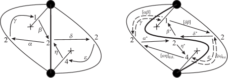
Figure 38. Configurations 25 and 30 of Figure 23. Left: $\tau$ and $Q(\tau,\omega)$. Right: $\sigma$ and $\widetilde{\mu}_{k}(Q(\tau,\omega))$. The numbers next to the arcs are the corresponding values of the tuple $\mathbf{d}(\tau,\omega)$.

1. We use the notation in Figure 38 and identify the quiver $Q(\sigma,\omega)$ with the subquiver of $\widetilde{\mu}_{k}(Q(\tau,\omega))$ obtained by deleting the dotted arrows in the figure.

2. The SP $(A(\sigma,\zeta),S(\sigma,\zeta))$ is the reduced part of $(\widetilde{\mu}_{k}(A(\tau,\xi)),S(\sigma,\zeta)^{\sharp})$, where

   $$S(\sigma,\zeta)^{\sharp} = \gamma[\alpha\beta]+\varepsilon[\delta\eta]_{g_{\delta}g_{\eta}}+\eta^{*}\alpha^{*}[\alpha\eta]_{g_{\alpha}g_{\eta}}+\beta^{*}\delta^{*}[\delta\beta]+S(\tau,\sigma)\in R\langle\langle\widetilde{\mu}_{k}(A(\tau,\xi))\rangle\rangle,$$

   with $S(\tau,\sigma)\in R\langle\langle A(\tau,\xi)\rangle\rangle\cap R\langle\langle A(\sigma,\zeta)\rangle\rangle$.

3. The potentials $S(\tau,\xi)$ and $\widetilde{\mu}_{k}(S(\tau,\xi))$ are

   $$S(\tau,\xi) = \alpha\beta\gamma+\delta\eta\varepsilon+S(\tau,\sigma)\ \ \ \ \ \text{and}$$

   $$\widetilde{\mu}_{k}(S(\tau,\xi)) \sim_{\operatorname{cyc}} \gamma[\alpha\beta]+\varepsilon[\delta\eta]_{g_{\delta}g_{\eta}}+\beta^{*}\alpha^{*}[\alpha\beta]+\pi_{(g_{\delta}g_{\eta})^{-1}}(\eta^{*}\delta^{*})[\delta\eta]_{g_{\delta}g_{\eta}}$$

   $$+\eta^{*}\alpha^{*}[\alpha\eta]_{g_{\alpha}g_{\eta}}+\beta^{*}\delta^{*}[\delta\beta]+S(\tau,\sigma),$$

   where $\pi_{(g_{\delta}g_{\eta})^{-1}}(x)=\frac{1}{2}\left(x+(g_{\delta}g_{\eta})^{-1}(u^{-1})xu\right)$.

4. From the equalities $g_{\alpha}g_{\beta}=g_{\gamma}^{-1}$, $g_{\delta}g_{\eta}=g_{\varepsilon}^{-1}$ and $\pi_{(g_{\alpha}g_{\beta})^{-1}}(\beta^{*}\alpha^{*})=\beta^{*}\alpha^{*}$, we deduce that the rule

   $\varphi$

   :

   $\gamma\mapsto\gamma-\beta^{*}\alpha^{*}$,

   $\varepsilon\mapsto\varepsilon-\pi_{(g_{\delta}g_{\eta})^{-1}}(\eta^{*}\delta^{*})$,

   produces a well-defined $R$-algebra automorphism $\varphi:R\langle\langle\widetilde{\mu}_{k}(A(\tau,\xi))\rangle\rangle\rightarrow R\langle\langle\widetilde{\mu}_{k}(A(\tau,\xi))\rangle\rangle$ (see [27, Propositions 2.15-(6) and 3.7]). It turns out to be obvious that $\varphi$ is a right-equivalence $(\widetilde{\mu}_{k}(A(\tau,\xi)),\widetilde{\mu}_{k}(S(\tau,\xi)))\rightarrow(\widetilde{\mu}_{k}(A(\tau,\xi)),S(\sigma,\zeta)^{\sharp})$.

Case 16.

Configurations 27 and 31.

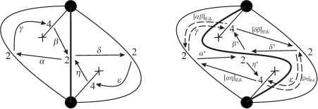
Figure 39. Configurations 27 and 31 of Figure 23. Left: $\tau$ and $Q(\tau,\omega)$. Right: $\sigma$ and $\widetilde{\mu}_{k}(Q(\tau,\omega))$. The numbers next to the arcs are the corresponding values of the tuple $\mathbf{d}(\tau,\omega)$.

1. We use the notation in Figure 39 and identify the quiver $Q(\sigma,\omega)$ with the subquiver of $\widetilde{\mu}_{k}(Q(\tau,\omega))$ obtained by deleting the dotted arrows in the figure.

2. The SP $(A(\sigma,\zeta),S(\sigma,\zeta))$ is the reduced part of $(\widetilde{\mu}_{k}(A(\tau,\xi)),S(\sigma,\zeta)^{\sharp})$, where

   $$S(\sigma,\zeta)^{\sharp} = \gamma[\alpha\beta]_{g_{\alpha}g_{\beta}}+\varepsilon[\delta\eta]_{g_{\delta}g_{\eta}}+\eta^{*}\alpha^{*}[\alpha\eta]_{g_{\alpha}g_{\eta}}+\beta^{*}\delta^{*}[\delta\beta]_{g_{\beta}g_{\delta}}+S(\tau,\sigma)\in R\langle\langle\widetilde{\mu}_{k}(A(\tau,\xi))\rangle\rangle,$$

   with $S(\tau,\sigma)\in R\langle\langle A(\tau,\xi)\rangle\rangle\cap R\langle\langle A(\sigma,\zeta)\rangle\rangle$.

3. The potentials $S(\tau,\xi)$ and $\widetilde{\mu}_{k}(S(\tau,\xi))$ are

   $$S(\tau,\xi) = \alpha\beta\gamma+\delta\eta\varepsilon+S(\tau,\sigma)\ \ \ \ \ \text{and}$$

   $$\widetilde{\mu}_{k}(S(\tau,\xi)) \sim_{\operatorname{cyc}} \gamma[\alpha\beta]_{g_{\alpha}g_{\beta}}+\varepsilon[\delta\eta]_{g_{\delta}g_{\eta}}$$

   $$+\pi_{(g_{\alpha}g_{\beta})^{-1}}(\beta^{*}\alpha^{*})[\alpha\beta]_{g_{\alpha}g_{\beta}}+\pi_{(g_{\delta}g_{\eta})^{-1}}(\eta^{*}\delta^{*})[\delta\eta]_{g_{\delta}g_{\eta}}$$

   $$+\eta^{*}\alpha^{*}[\alpha\eta]_{g_{\alpha}g_{\eta}}+\beta^{*}\delta^{*}[\delta\eta]_{g_{\delta}g_{\eta}}+S(\tau,\sigma).$$

4. From the equalities $g_{\alpha}g_{\beta}=g_{\gamma}^{-1}$ and $g_{\delta}g_{\eta}=g_{\varepsilon}^{-1}$, we deduce that the rule

   $\varphi$

   :

   $\gamma\mapsto\gamma-\pi_{(g_{\alpha}g_{\beta})^{-1}}(\beta^{*}\alpha^{*})$,

   $\varepsilon\mapsto\varepsilon-\pi_{(g_{\delta}g_{\eta})^{-1}}(\eta^{*}\delta^{*})$,

   produces a well-defined $R$-algebra automorphism $\varphi:R\langle\langle\widetilde{\mu}_{k}(A(\tau,\xi))\rangle\rangle\rightarrow R\langle\langle\widetilde{\mu}_{k}(A(\tau,\xi))\rangle\rangle$ (see [27, Propositions 2.15-(6) and 3.7]). It turns out to be obvious that $\varphi$ is a right-equivalence $(\widetilde{\mu}_{k}(A(\tau,\xi)),\widetilde{\mu}_{k}(S(\tau,\xi)))\rightarrow(\widetilde{\mu}_{k}(A(\tau,\xi)),S(\sigma,\zeta)^{\sharp})$.

Case 17.

Configurations 32 and 40.

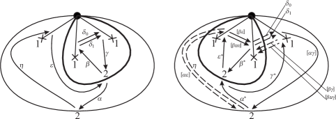
Figure 40. Configurations 32 and 40 of Figure 23. Left: $\tau$ and $Q(\tau,\omega)$. Right: $\sigma$ and $\widetilde{\mu}_{k}(Q(\tau,\omega))$. The numbers next to the arcs are the corresponding values of the tuple $\mathbf{d}(\tau,\omega)$.

1. We use the notation in Figure 40 and identify the quiver $Q(\sigma,\omega)$ with the subquiver of $\widetilde{\mu}_{k}(Q(\tau,\omega))$ obtained by deleting the dotted arrows in the figure.

2. The SP $(A(\sigma,\zeta),S(\sigma,\zeta))$ is the reduced part of $(\widetilde{\mu}_{k}(A(\tau,\xi)),S(\sigma,\zeta)^{\sharp})$, where

   $$S(\sigma,\zeta)^{\sharp} = \delta_{0}[\beta\gamma]+\delta_{1}[\beta u\gamma]+\eta[\alpha\varepsilon]+\alpha^{*}[\alpha\gamma]\gamma^{*}+[\beta\varepsilon]\varepsilon^{*}u\beta^{*}+[\beta u\varepsilon]\varepsilon^{*}\beta^{*}+S(\tau,\sigma)\in R\langle\langle\widetilde{\mu}_{k}(A(\tau,\xi))\rangle\rangle,$$

   with $S(\tau,\sigma)\in R\langle\langle A(\tau,\xi)\rangle\rangle\cap R\langle\langle A(\sigma,\zeta)\rangle\rangle$.

3. The potentials $S(\tau,\xi)$ and $\widetilde{\mu}_{k}(S(\tau,\xi))$ are

   $$S(\tau,\xi) = \delta_{0}\beta\gamma+\delta_{1}\beta u\gamma+\eta\alpha\varepsilon+S(\tau,\sigma)\ \ \ \ \ \text{and}$$

   $$\widetilde{\mu}_{k}(S(\tau,\xi)) = \delta_{0}[\beta\gamma]+\delta_{1}[\beta u\gamma]+\eta[\alpha\varepsilon]$$

   $$+\gamma^{*}\beta^{*}[\beta\gamma]+\gamma^{*}u^{-1}\beta^{*}[\beta u\gamma]+\varepsilon^{*}\alpha^{*}[\alpha\varepsilon]+\alpha^{*}[\alpha\gamma]\gamma^{*}+[\beta\varepsilon]\varepsilon^{*}\beta^{*}+[\beta u\varepsilon]\varepsilon^{*}u^{-1}\beta^{*}+S(\tau,\sigma).$$

4. The rules

   $\varphi$	:	$\delta_{0}\mapsto\delta_{0}-\gamma^{*}\beta^{*}$,	$\delta_{1}\mapsto\delta_{1}-\gamma^{*}u^{-1}\beta^{*}$,	$\eta\mapsto\eta-\varepsilon^{*}\alpha^{*}$,
   $\Phi$	:	$\varepsilon^{*}\mapsto\varepsilon^{*}u$

   produce a well-defined $R$-algebra automorphisms $\varphi,\Phi:R\langle\langle\widetilde{\mu}_{k}(A(\tau,\xi))\rangle\rangle\rightarrow R\langle\langle\widetilde{\mu}_{k}(A(\tau,\xi))\rangle\rangle$ (see [27, Propositions 2.15-(6) and 3.7]). It turns out to be obvious that the composition $\Phi\varphi$ is a right-equivalence $(\widetilde{\mu}_{k}(A(\tau,\xi)),\widetilde{\mu}_{k}(S(\tau,\xi)))\rightarrow(\widetilde{\mu}_{k}(A(\tau,\xi)),S(\sigma,\zeta)^{\sharp})$.

Case 18.

Configurations 33 and 44.

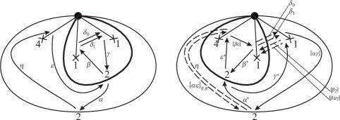
Figure 41. Configurations 33 and 44 of Figure 23. Left: $\tau$ and $Q(\tau,\omega)$. Right: $\sigma$ and $\widetilde{\mu}_{k}(Q(\tau,\omega))$. The numbers next to the arcs are the corresponding values of the tuple $\mathbf{d}(\tau,\omega)$.

1. We use the notation in Figure 41 and identify the quiver $Q(\sigma,\omega)$ with the subquiver of $\widetilde{\mu}_{k}(Q(\tau,\omega))$ obtained by deleting the dotted arrows in the figure.

2. The SP $(A(\sigma,\zeta),S(\sigma,\zeta))$ is the reduced part of $(\widetilde{\mu}_{k}(A(\tau,\xi)),S(\sigma,\zeta)^{\sharp})$, where

   $$S(\sigma,\zeta)^{\sharp} = \delta_{0}[\beta\gamma]+\delta_{1}[\beta u\gamma]+\eta[\alpha\varepsilon]_{g_{\alpha}g_{\varepsilon}}+\beta^{*}[\beta\varepsilon]\varepsilon^{*}+\alpha^{*}[\alpha\gamma]\gamma^{*}+S(\tau,\sigma)\in R\langle\langle\widetilde{\mu}_{k}(A(\tau,\xi))\rangle\rangle,$$

   with $S(\tau,\sigma)\in R\langle\langle A(\tau,\xi)\rangle\rangle\cap R\langle\langle A(\sigma,\zeta)\rangle\rangle$.

3. The potentials $S(\tau,\xi)$ and $\widetilde{\mu}_{k}(S(\tau,\xi))$ are

   $$S(\tau,\xi) = \delta_{0}\beta\gamma+\delta_{1}\beta u\gamma+\eta\alpha\varepsilon+S(\tau,\sigma)\ \ \ \ \ \text{and}$$

   $$\widetilde{\mu}_{k}(S(\tau,\xi)) \sim_{\operatorname{cyc}} \delta_{0}[\beta\gamma]+\delta_{1}[\beta u\gamma]+\eta[\alpha\varepsilon]_{g_{\alpha}g_{\varepsilon}}$$

   $$+\gamma^{*}\beta^{*}[\beta\gamma]+\gamma^{*}u^{-1}\beta^{*}[\beta u\gamma]+\pi_{(g_{\alpha}g_{\varepsilon})^{-1}}(\varepsilon^{*}\alpha^{*})[\alpha\varepsilon]_{g_{\alpha}g_{\varepsilon}}$$

   $$+\alpha^{*}[\alpha\gamma]\gamma^{*}+\beta^{*}[\beta\varepsilon]\varepsilon^{*}+S(\tau,\sigma),$$

   where $\pi_{(g_{\alpha}g_{\varepsilon})^{-1}}(x)=\frac{1}{2}\left(x+(g_{\alpha}g_{\varepsilon})^{-1}(u^{-1})xu\right)$.

4. From the equality $(g_{\alpha}g_{\varepsilon})^{-1}=g_{\eta}$, we deduce that the rule

   $\varphi$

   :

   $\delta_{0}\mapsto\delta_{0}-\gamma^{*}\beta^{*}$,

   $\delta_{1}\mapsto\delta_{1}-\gamma^{*}u^{-1}\beta^{*}$,

   $\eta\mapsto\eta-\pi_{(g_{\alpha}g_{\varepsilon})^{-1}}(\varepsilon^{*}\alpha^{*})$

   produces a well-defined $R$-algebra automorphism $\varphi:R\langle\langle\widetilde{\mu}_{k}(A(\tau,\xi))\rangle\rangle\rightarrow R\langle\langle\widetilde{\mu}_{k}(A(\tau,\xi))\rangle\rangle$ (see [27, Propositions 2.15-(6) and 3.7]). It turns out to be obvious that $\varphi$ is a right-equivalence $(\widetilde{\mu}_{k}(A(\tau,\xi)),\widetilde{\mu}_{k}(S(\tau,\xi)))\rightarrow(\widetilde{\mu}_{k}(A(\tau,\xi)),S(\sigma,\zeta)^{\sharp})$.

Case 19.

Configurations 34 and 41.

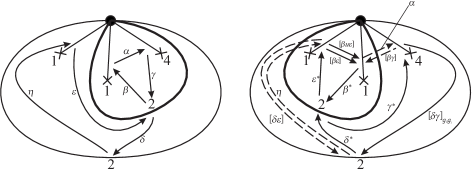
Figure 42. Configurations 34 and 41 of Figure 23. Left: $\tau$ and $Q(\tau,\omega)$. Right: $\sigma$ and $\widetilde{\mu}_{k}(Q(\tau,\omega))$. The numbers next to the arcs are the corresponding values of the tuple $\mathbf{d}(\tau,\omega)$.

1. We use the notation in Figure 42 and identify the quiver $Q(\sigma,\omega)$ with the subquiver of $\widetilde{\mu}_{k}(Q(\tau,\omega))$ obtained by deleting the dotted arrows in the figure.

2. The SP $(A(\sigma,\zeta),S(\sigma,\zeta))$ is the reduced part of $(\widetilde{\mu}_{k}(A(\tau,\xi)),S(\sigma,\zeta)^{\sharp})$, where

   $$S(\sigma,\zeta)^{\sharp} = \alpha[\beta\gamma]+\eta[\delta\varepsilon]+[\beta\varepsilon]\varepsilon^{*}u\beta^{*}+[\beta u\varepsilon]\varepsilon^{*}\beta^{*}+\delta^{*}[\delta\gamma]_{g_{\delta}g_{\gamma}}\gamma^{*}+S(\tau,\sigma)\in R\langle\langle\widetilde{\mu}_{k}(A(\tau,\xi))\rangle\rangle,$$

   with $S(\tau,\sigma)\in R\langle\langle A(\tau,\xi)\rangle\rangle\cap R\langle\langle A(\sigma,\zeta)\rangle\rangle$.

3. The potentials $S(\tau,\xi)$ and $\widetilde{\mu}_{k}(S(\tau,\xi))$ are

   $$S(\tau,\xi) = \alpha\beta\gamma+\eta\delta\varepsilon+S(\tau,\sigma)\ \ \ \ \ \text{and}$$

   $$\widetilde{\mu}_{k}(S(\tau,\xi)) = \alpha[\beta\gamma]+\eta[\delta\varepsilon]$$

   $$+\gamma^{*}\beta^{*}[\beta\gamma]+\varepsilon^{*}\delta^{*}[\delta\varepsilon]+[\beta\varepsilon]\varepsilon^{*}\beta^{*}+[\beta u\varepsilon]\varepsilon^{*}u^{-1}\beta^{*}+\delta^{*}[\delta\gamma]_{g_{\delta}g_{\gamma}}\gamma^{*}+S(\tau,\sigma).$$

4. The rules

   $\varphi$

   :

   $\alpha\mapsto\alpha-\gamma^{*}\beta^{*}$,

   $\eta\mapsto\eta-\varepsilon^{*}\delta^{*}$,

   and

   $\Phi$

   :

   $\varepsilon^{*}\mapsto\varepsilon^{*}u$

   produce well-defined $R$-algebra automorphisms $\varphi,\Phi:R\langle\langle\widetilde{\mu}_{k}(A(\tau,\xi))\rangle\rangle\rightarrow R\langle\langle\widetilde{\mu}_{k}(A(\tau,\xi))\rangle\rangle$ (see [27, Propositions 2.15-(6) and 3.7]). It turns out to be obvious that the composition $\Phi\varphi$ is a right-equivalence $(\widetilde{\mu}_{k}(A(\tau,\xi)),\widetilde{\mu}_{k}(S(\tau,\xi)))\rightarrow(\widetilde{\mu}_{k}(A(\tau,\xi)),S(\sigma,\zeta)^{\sharp})$.

Case 20.

Configurations 35 and 45.

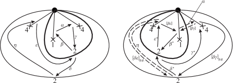
Figure 43. Configurations 35 and 45 of Figure 23. Left: $\tau$ and $Q(\tau,\omega)$. Right: $\sigma$ and $\widetilde{\mu}_{k}(Q(\tau,\omega))$. The numbers next to the arcs are the corresponding values of the tuple $\mathbf{d}(\tau,\omega)$.

1. We use the notation in Figure 43 and identify the quiver $Q(\sigma,\omega)$ with the subquiver of $\widetilde{\mu}_{k}(Q(\tau,\omega))$ obtained by deleting the dotted arrows in the figure.

2. The SP $(A(\sigma,\zeta),S(\sigma,\zeta))$ is the reduced part of $(\widetilde{\mu}_{k}(A(\tau,\xi)),S(\sigma,\zeta)^{\sharp})$, where

   $$S(\sigma,\zeta)^{\sharp} = \alpha[\beta\gamma]+\eta[\delta\varepsilon]_{g_{\delta}g_{\varepsilon}}+\beta^{*}[\beta\varepsilon]\varepsilon^{*}+\delta^{*}[\delta\gamma]_{g_{\delta}g_{\gamma}}\gamma^{*}+S(\tau,\sigma)\in R\langle\langle\widetilde{\mu}_{k}(A(\tau,\xi))\rangle\rangle,$$

   with $S(\tau,\sigma)\in R\langle\langle A(\tau,\xi)\rangle\rangle\cap R\langle\langle A(\sigma,\zeta)\rangle\rangle$.

3. The potentials $S(\tau,\xi)$ and $\widetilde{\mu}_{k}(S(\tau,\xi))$ are

   $$S(\tau,\xi) = \alpha\beta\gamma+\eta\delta\varepsilon+S(\tau,\sigma)\ \ \ \ \ \text{and}$$

   $$\widetilde{\mu}_{k}(S(\tau,\xi)) \sim_{\operatorname{cyc}} \alpha[\beta\gamma]+\eta[\delta\varepsilon]_{g_{\delta}g_{\varepsilon}}$$

   $$+\gamma^{*}\beta^{*}[\beta\gamma]+\pi_{(g_{\delta}g_{\varepsilon})^{-1}}(\varepsilon^{*}\delta^{*})[\delta\varepsilon]_{g_{\delta}g_{\varepsilon}}+\beta^{*}[\beta\varepsilon]\varepsilon^{*}+\delta^{*}[\delta\gamma]_{g_{\delta}g_{\gamma}}\gamma^{*}+S(\tau,\sigma).$$

4. From the equality $(g_{\delta}g_{\varepsilon})^{-1}=g_{\eta}$, we deduce that the rule

   $\varphi$

   :

   $\alpha\mapsto\alpha-\gamma^{*}\beta^{*}$,

   $\eta\mapsto\eta-\pi_{(g_{\delta}g_{\varepsilon})^{-1}}(\varepsilon^{*}\delta^{*})$,

   produces a well-defined $R$-algebra automorphism $\varphi:R\langle\langle\widetilde{\mu}_{k}(A(\tau,\xi))\rangle\rangle\rightarrow R\langle\langle\widetilde{\mu}_{k}(A(\tau,\xi))\rangle\rangle$ (see [27, Propositions 2.15-(6) and 3.7]). It turns out to be obvious that $\varphi$ is a right-equivalence $(\widetilde{\mu}_{k}(A(\tau,\xi)),\widetilde{\mu}_{k}(S(\tau,\xi)))\rightarrow(\widetilde{\mu}_{k}(A(\tau,\xi)),S(\sigma,\zeta)^{\sharp})$.

Case 21.

Configurations 36 and 42.

Figure 44. Configurations 36 and 42 of Figure 23. Left: $\tau$ and $Q(\tau,\omega)$. Right: $\sigma$ and $\widetilde{\mu}_{k}(Q(\tau,\omega))$. The numbers next to the arcs are the corresponding values of the tuple $\mathbf{d}(\tau,\omega)$.

1. We use the notation in Figure 44 and identify the quiver $Q(\sigma,\omega)$ with the subquiver of $\widetilde{\mu}_{k}(Q(\tau,\omega))$ obtained by deleting the dotted arrows in the figure.

2. The SP $(A(\sigma,\zeta),S(\sigma,\zeta))$ is the reduced part of $(\widetilde{\mu}_{k}(A(\tau,\xi)),S(\sigma,\zeta)^{\sharp})$, where

   $$S(\sigma,\zeta)^{\sharp} = \alpha[\beta\gamma]+\eta[\delta\varepsilon]+\beta^{*}[\beta\varepsilon]\varepsilon^{*}+\delta^{*}[\delta\gamma]\gamma^{*}+S(\tau,\sigma)\in R\langle\langle\widetilde{\mu}_{k}(A(\tau,\xi))\rangle\rangle,$$

   with $S(\tau,\sigma)\in R\langle\langle A(\tau,\xi)\rangle\rangle\cap R\langle\langle A(\sigma,\zeta)\rangle\rangle$.

3. The potentials $S(\tau,\xi)$ and $\widetilde{\mu}_{k}(S(\tau,\xi))$ are

   $$S(\tau,\xi) = \alpha\beta\gamma+\eta\delta\varepsilon+S(\tau,\sigma)\ \ \ \ \ \text{and}$$

   $$\widetilde{\mu}_{k}(S(\tau,\xi)) = \alpha[\beta\gamma]+\eta[\delta\varepsilon]$$

   $$+\gamma^{*}\beta^{*}[\beta\gamma]+\varepsilon^{*}\delta^{*}[\delta\varepsilon]+\beta^{*}[\beta\varepsilon]\varepsilon^{*}+\delta^{*}[\delta\gamma]\gamma^{*}+S(\tau,\sigma).$$

4. The rule

   $\varphi$

   :

   $\alpha\mapsto\alpha-\gamma^{*}\beta^{*}$,

   $\eta\mapsto\eta-\varepsilon^{*}\delta^{*}$,

   produces a well-defined $R$-algebra automorphism $\varphi:R\langle\langle\widetilde{\mu}_{k}(A(\tau,\xi))\rangle\rangle\rightarrow R\langle\langle\widetilde{\mu}_{k}(A(\tau,\xi))\rangle\rangle$ (see [27, Propositions 2.15-(6) and 3.7]). It turns out to be obvious that $\varphi$ is a right-equivalence $(\widetilde{\mu}_{k}(A(\tau,\xi)),\widetilde{\mu}_{k}(S(\tau,\xi)))\rightarrow(\widetilde{\mu}_{k}(A(\tau,\xi)),S(\sigma,\zeta)^{\sharp})$.

Case 22.

Configurations 37 and 46.

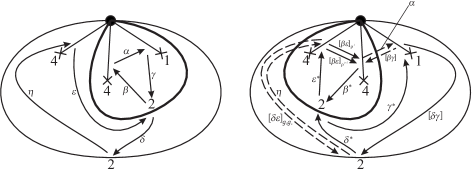
Figure 45. Configurations 37 and 46 of Figure 23. Left: $\tau$ and $Q(\tau,\omega)$. Right: $\sigma$ and $\widetilde{\mu}_{k}(Q(\tau,\omega))$. The numbers next to the arcs are the corresponding values of the tuple $\mathbf{d}(\tau,\omega)$.

1. We use the notation in Figure 45, where the element $j\in\{0,1,2,3\}$ satisfies $\rho^{j}|_{L}=g_{\beta}g_{\varepsilon}=\rho^{j+2}|_{L}$. Furthermore, we identify the quiver $Q(\sigma,\omega)$ with the subquiver of $\widetilde{\mu}_{k}(Q(\tau,\omega))$ obtained by deleting the dotted arrows in the figure. By the definition of the modulating function $\widetilde{\mu}_{k}(g):\widetilde{\mu}_{k}(Q(\tau,\xi))_{1}\rightarrow\bigcup_{i,j\in\tau}G_{i,j}$ (cf. [27, Definition 3.19]), we have

   $\widetilde{\mu}_{k}(g)([\delta\varepsilon]_{g_{\delta}g_{\varepsilon}})=g_{\delta}g_{\varepsilon}$,

   $\widetilde{\mu}_{k}(g)([\beta\varepsilon]_{\rho^{j}})=\rho^{j}$

   and

   $\widetilde{\mu}_{k}(g)([\beta\varepsilon]_{\rho^{j+2}})=\rho^{j+2}$,

   which respectively coincide with $\theta^{\zeta([\delta\varepsilon]_{g_{\delta}g_{\varepsilon}})}$, $g(\sigma,\zeta)_{[\beta\varepsilon]_{\rho^{j}}}$ and $g(\sigma,\zeta)_{[\beta\varepsilon]_{\rho^{j+2}}}$ since $(\sigma,\zeta)=f_{k}(\tau,\xi)$.

2. The SP $(A(\sigma,\zeta),S(\sigma,\zeta))$ is the reduced part of $(\widetilde{\mu}_{k}(A(\tau,\xi)),S(\sigma,\zeta)^{\sharp})$, where

   $$S(\sigma,\zeta)^{\sharp} = \alpha[\beta\gamma]+\eta[\delta\varepsilon]_{g_{\delta}g_{\varepsilon}}+([\beta\varepsilon]_{\rho^{j}}+[\beta\varepsilon]_{\rho^{j+2}})\varepsilon^{*}\beta^{*}+\delta^{*}[\delta\gamma]\gamma^{*}+S(\tau,\sigma)\in R\langle\langle\widetilde{\mu}_{k}(A(\tau,\xi))\rangle\rangle,$$

   with $S(\tau,\sigma)\in R\langle\langle A(\tau,\xi)\rangle\rangle\cap R\langle\langle A(\sigma,\zeta)\rangle\rangle$.

3. The potentials $S(\tau,\xi)$ and $\widetilde{\mu}_{k}(S(\tau,\xi))$ are Furthermore,

   $$S(\tau,\xi) = \alpha\beta\gamma+\eta\delta\varepsilon+S(\tau,\sigma)\ \ \ \ \ \text{and}$$

   $$\widetilde{\mu}_{k}(S(\tau,\xi)) \sim_{\operatorname{cyc}} \alpha[\beta\gamma]+\eta[\delta\varepsilon]_{g_{\delta}g_{\varepsilon}}$$

   $$\gamma^{*}\beta^{*}[\beta\gamma]+\pi_{(g_{\delta}g_{\varepsilon})^{-1}}(\varepsilon^{*}\delta^{*})[\delta\varepsilon]_{g_{\delta}g_{\varepsilon}}+([\beta\varepsilon]_{\rho^{j}}+[\beta\varepsilon]_{\rho^{j+2}})\varepsilon^{*}\beta^{*}+\delta^{*}[\delta\gamma]\gamma^{*}+S(\tau,\sigma).$$

4. From the equality $(g_{\delta}g_{\varepsilon})^{-1}=g_{\eta}$, we deduce that the rule

   $\varphi$

   :

   $\alpha\mapsto\alpha-\gamma^{*}\beta^{*}$,

   $\eta\mapsto\eta-\pi_{(g_{\delta}g_{\varepsilon})^{-1}}(\varepsilon^{*}\delta^{*})$,

   produces a well-defined $R$-algebra automorphism $\varphi:R\langle\langle\widetilde{\mu}_{k}(A(\tau,\xi))\rangle\rangle\rightarrow R\langle\langle\widetilde{\mu}_{k}(A(\tau,\xi))\rangle\rangle$ (see [27, Propositions 2.15-(6) and 3.7]). It turns out to be obvious that $\varphi$ is a right-equivalence $(\widetilde{\mu}_{k}(A(\tau,\xi)),\widetilde{\mu}_{k}(S(\tau,\xi)))\rightarrow(\widetilde{\mu}_{k}(A(\tau,\xi)),S(\sigma,\zeta)^{\sharp})$.

Case 23.

Configurations 38 and 43.

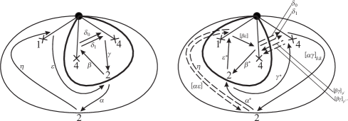
Figure 46. Configurations 38 and 43 of Figure 23. Left: $\tau$ and $Q(\tau,\omega)$. Right: $\sigma$ and $\widetilde{\mu}_{k}(Q(\tau,\omega))$. The numbers next to the arcs are the corresponding values of the tuple $\mathbf{d}(\tau,\omega)$.

1. We use the notation in Figure 46, where $j$ is the unique element of $\{0,1\}$ that satisfies $\rho^{j}|_{L}=g_{\beta}g_{\gamma}=\rho^{j+2}|_{L}$. Furthermore, we identify the quiver $Q(\sigma,\omega)$ with the subquiver of $\widetilde{\mu}_{k}(Q(\tau,\omega))$ obtained by deleting the dotted arrows in the figure.

   By the definition of the modulating function $\widetilde{\mu}_{k}(g):\widetilde{\mu}_{k}(Q(\tau,\xi))_{1}\rightarrow\bigcup_{i,j\in\tau}G_{i,j}$ (cf. [27, Definition 3.19]), we have

   $\widetilde{\mu}_{k}(g)([\alpha\gamma]_{g_{\alpha}g_{\gamma}})=g_{\alpha}g_{\gamma}$,

   $\widetilde{\mu}_{k}(g)([\beta\gamma]_{\rho^{j}})=\rho^{j}$

   and

   $\widetilde{\mu}_{k}(g)([\beta\gamma]_{\rho^{j+2}})=\rho^{j+2}$,

   which respectively coincide with $\theta^{\zeta([\alpha\gamma]_{g_{\alpha}g_{\gamma}})}$, $g(\sigma,\zeta)_{[\beta\gamma]_{\rho^{j}}}$ and $g(\sigma,\zeta)_{[\beta\gamma]_{\rho^{j+2}}}$ since $(\sigma,\zeta)=f_{k}(\tau,\xi)$.

   Let $\ell$ be the unique element of $\{0,1\}$ whose congruence class modulo $2$ is $\xi(\delta_{0})$. By the definition of the modulating function $g$ (Definition 6.1), we have

   $g_{\delta_{0}}=\rho^{\ell}$,

   $g_{\delta_{1}}=\rho^{\ell+2}$.

   On the other hand, since $\xi$ is a 1-cocycle we have $\xi([\delta_{0}])=-\xi([\beta])-\xi([\gamma])$, hence $\rho^{\ell}|_{L}=\rho^{\ell+2}|_{L}=\theta^{\xi([\delta_{0}])}=\theta^{-\xi([\beta])-\xi([\gamma])}=(g_{\beta}g_{\gamma})^{-1}=(\rho^{j}|_{L})^{-1}=(\rho^{j+2}|_{L})^{-1}$ (we have used the definition of $g_{\beta}$ and $g_{\gamma}$ in terms of $\xi$), and therefore, $\{\rho^{\ell},\rho^{\ell+2}\}=\{(\rho^{j})^{-1},(\rho^{j+2})^{-1}\}$. In particular, $\ell=j$ and

   $g_{\delta_{j}}=\rho^{-j}$,

   $g_{\delta_{|j-1|}}=\rho^{-j-2}$.

2. The SP $(A(\sigma,\zeta),S(\sigma,\zeta))$ is the reduced part of $(\widetilde{\mu}_{k}(A(\tau,\xi)),S(\sigma,\zeta)^{\sharp})$, where

   $$S(\sigma,\zeta)^{\sharp} = \delta_{j}[\beta\gamma]_{\rho^{j}}+\delta_{|j-1|}[\beta\gamma]_{\rho^{j+2}}+\eta[\alpha\varepsilon]+\beta^{*}[\beta\varepsilon]\varepsilon^{*}+\alpha^{*}[\alpha\gamma]_{g_{\alpha}g_{\gamma}}\gamma^{*}+S(\tau,\sigma)\in R\langle\langle\widetilde{\mu}_{k}(A(\tau,\xi))\rangle\rangle,$$

   with $S(\tau,\sigma)\in R\langle\langle A(\tau,\xi)\rangle\rangle\cap R\langle\langle A(\sigma,\zeta)\rangle\rangle$.

3. The potentials $S(\tau,\xi)$ and $\widetilde{\mu}_{k}(S(\tau,\xi))$ are

   $$S(\tau,\xi) = (\delta_{0}+\delta_{1})\beta\gamma+\eta\alpha\varepsilon+S(\tau,\sigma)\ \ \ \ \ \text{and}$$

   $$\widetilde{\mu}_{k}(S(\tau,\xi)) \sim_{\operatorname{cyc}} \delta_{j}[\beta\gamma]_{\rho^{j}}+\delta_{|j-1|}[\beta\gamma]_{\rho^{j+2}}+\eta[\alpha\varepsilon]$$

   $$+\pi_{\rho^{-j}}(\gamma^{*}\beta^{*})[\beta\gamma]_{\rho^{j}}+\pi_{\rho^{-j-2}}(\gamma^{*}\beta^{*})[\beta\gamma]_{\rho^{j+2}}+\varepsilon^{*}\alpha^{*}[\alpha\varepsilon]$$

   $$+\beta^{*}[\beta\varepsilon]\varepsilon^{*}+\alpha^{*}[\alpha\gamma]_{g_{\alpha}g_{\gamma}}\gamma^{*}+S(\tau,\sigma).$$

4. From the equalities $g_{\delta_{j}}=\rho^{-j}$ and $g_{\delta_{|j-1|}}=\rho^{-j-2}$, we deduce that the rule

   $\varphi$

   :

   $\delta_{j}\mapsto\delta_{j}-\pi_{\rho^{-j}}(\gamma^{*}\beta^{*})$,

   $\delta_{|j-1|}\mapsto\delta_{|j-1|}-\pi_{\rho^{-j-2}}(\gamma^{*}\beta^{*})$,

   $\eta\mapsto\eta-\varepsilon^{*}\alpha^{*}$,

   produces a well-defined $R$-algebra automorphism $\varphi:R\langle\langle\widetilde{\mu}_{k}(A(\tau,\xi))\rangle\rangle\rightarrow R\langle\langle\widetilde{\mu}_{k}(A(\tau,\xi))\rangle\rangle$ (see [27, Propositions 2.15-(6) and 3.7]). It turns out to be obvious that $\varphi$ is a right-equivalence $(\widetilde{\mu}_{k}(A(\tau,\xi)),\widetilde{\mu}_{k}(S(\tau,\xi)))\rightarrow(\widetilde{\mu}_{k}(A(\tau,\xi)),S(\sigma,\zeta)^{\sharp})$.

Case 24.

Configurations 39 and 47.

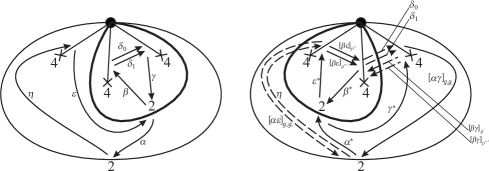
Figure 47. Configurations 39 and 47 of Figure 23. Left: $\tau$ and $Q(\tau,\omega)$. Right: $\sigma$ and $\widetilde{\mu}_{k}(Q(\tau,\omega))$. The numbers next to the arcs are the corresponding values of the tuple $\mathbf{d}(\tau,\omega)$.

1. We use the notation in Figure 47, where $j$ (resp. $m$) is the unique element of $\{0,1\}$ that satisfies $\rho^{j}|_{L}=g_{\beta}g_{\gamma}=\rho^{j+2}|_{L}$ (resp. $\rho^{m}|_{L}=g_{\beta}g_{\varepsilon}=\rho^{m+2}|_{L}$). Furthermore, we identify the quiver $Q(\sigma,\omega)$ with the subquiver of $\widetilde{\mu}_{k}(Q(\tau,\omega))$ obtained by deleting the dotted arrows in the figure.

   By the definition of the modulating function $\widetilde{\mu}_{k}(g):\widetilde{\mu}_{k}(Q(\tau,\xi))_{1}\rightarrow\bigcup_{i,j\in\tau}G_{i,j}$ (cf. [27, Definition 3.19]), we have

   $\widetilde{\mu}_{k}(g)([\alpha\gamma]_{g_{\alpha}g_{\gamma}})=g_{\alpha}g_{\gamma}$,	$\widetilde{\mu}_{k}(g)([\beta\gamma]_{\rho^{j}})=\rho^{j}$,	$\widetilde{\mu}_{k}(g)([\beta\gamma]_{\rho^{j+2}})=\rho^{j+2}$,
   $\widetilde{\mu}_{k}(g)([\beta\varepsilon]_{\rho^{m}})=\rho^{m}$	and	$\widetilde{\mu}_{k}(g)([\beta\varepsilon]_{\rho^{m+2}})=\rho^{m+2}$,

   which respectively coincide with $\theta^{\zeta([\alpha\gamma]_{g_{\alpha}g_{\gamma}})}$, $g(\sigma,\zeta)_{[\beta\gamma]_{\rho^{j}}}$ and $g(\sigma,\zeta)_{[\beta\gamma]_{\rho^{j+2}}}$ since $(\sigma,\zeta)=f_{k}(\tau,\xi)$.

   Let $\ell$ be the unique element of $\{0,1\}$ whose congruence class modulo $2$ is $\xi(\delta_{0})$. By the definition of the modulating function $g$ (Definition 6.1), we have

   $g_{\delta_{0}}=\rho^{\ell}$,

   $g_{\delta_{1}}=\rho^{\ell+2}$.

   On the other hand, since $\xi$ is a 1-cocycle we have $\xi([\delta_{0}])=-\xi([\beta])-\xi([\gamma])$, hence $\rho^{\ell}|_{L}=\rho^{\ell+2}|_{L}=\theta^{\xi([\delta_{0}])}=\theta^{-\xi([\beta])-\xi([\gamma])}=(g_{\beta}g_{\gamma})^{-1}=(\rho^{j}|_{L})^{-1}=(\rho^{j+2}|_{L})^{-1}$ (we have used the definition of $g_{\beta}$ and $g_{\gamma}$ in terms of $\xi$), and therefore, $\{\rho^{\ell},\rho^{\ell+2}\}=\{(\rho^{j})^{-1},(\rho^{j+2})^{-1}\}$. In particular, $\ell=j$ and

   $g_{\delta_{j}}=\rho^{-j}$,

   $g_{\delta_{|j-1|}}=\rho^{-j-2}$.

2. The SP $(A(\sigma,\zeta),S(\sigma,\zeta))$ is the reduced part of $(\widetilde{\mu}_{k}(A(\tau,\xi)),S(\sigma,\zeta)^{\sharp})$, where

   $$S(\sigma,\zeta)^{\sharp} = \delta_{j}[\beta\gamma]_{\rho^{j}}+\delta_{|j-1|}[\beta\gamma]_{\rho^{j+2}}+\eta[\alpha\varepsilon]_{g_{\alpha}g_{\varepsilon}}+\beta^{*}[\beta\varepsilon]_{\rho^{m}}\varepsilon^{*}+\beta^{*}[\beta\varepsilon]_{\rho^{m+2}}\varepsilon^{*}+\alpha^{*}[\alpha\gamma]_{g_{\alpha}g_{\gamma}}\gamma^{*}+S(\tau,\sigma)\in R\langle\langle\widetilde{\mu}_{k}(A(\tau,\xi))\rangle\rangle,$$

   with $S(\tau,\sigma)\in R\langle\langle A(\tau,\xi)\rangle\rangle\cap R\langle\langle A(\sigma,\zeta)\rangle\rangle$.

3. The potentials $S(\tau,\xi)$ and $\widetilde{\mu}_{k}(S(\tau,\xi))$ are

   $$S(\tau,\xi) = (\delta_{0}+\delta_{1})\beta\gamma+\eta\alpha\varepsilon+S(\tau,\sigma)\ \ \ \ \ \text{and}$$

   $$\widetilde{\mu}_{k}(S(\tau,\xi)) \sim_{\operatorname{cyc}} (\delta_{0}+\delta_{1})([\beta\gamma]_{\rho^{j}}+[\beta\gamma]_{\rho^{j+2}})+\eta[\alpha\varepsilon]_{g_{\alpha}g_{\varepsilon}}$$

   $$+\gamma^{*}\beta^{*}[\beta\gamma]_{\rho^{j}}+\gamma^{*}\beta^{*}[\beta\gamma]_{\rho^{j+2}}+\varepsilon^{*}\alpha^{*}[\alpha\varepsilon]_{g_{\alpha}g_{\varepsilon}}+\beta^{*}[\beta\varepsilon]_{\rho^{m}}\varepsilon^{*}+\beta^{*}[\beta\varepsilon]_{\rho^{m+2}}\varepsilon^{*}+\alpha^{*}[\alpha\gamma]_{g_{\alpha}g_{\gamma}}\gamma^{*}+S(\tau,\sigma)$$

   $$\sim_{\operatorname{cyc}} \delta_{j}[\beta\gamma]_{\rho^{j}}+\delta_{|j-1|}[\beta\gamma]_{\rho^{j+2}}+\eta[\alpha\varepsilon]_{g_{\alpha}g_{\varepsilon}}$$

   $$+\pi_{\rho^{-j}}(\gamma^{*}\beta^{*})[\beta\gamma]_{\rho^{j}}+\pi_{\rho^{-j-2}}(\gamma^{*}\beta^{*})[\beta\gamma]_{\rho^{j+2}}+\pi_{(g_{\alpha}g_{\varepsilon})^{-1}}(\varepsilon^{*}\alpha^{*})[\alpha\varepsilon]_{g_{\alpha}g_{\varepsilon}}$$

   $$+\beta^{*}[\beta\varepsilon]_{\rho^{m}}\varepsilon^{*}+\beta^{*}[\beta\varepsilon]_{\rho^{m+2}}\varepsilon^{*}+\alpha^{*}[\alpha\gamma]_{g_{\alpha}g_{\gamma}}\gamma^{*}+S(\tau,\sigma).$$

4. From the equalities $g_{\delta_{j}}=\rho^{-j}$, $g_{\delta_{|j-1|}}=\rho^{-j-2}$ and $(g_{\alpha}g_{\varepsilon})^{-1}=g_{\eta}$, we deduce that the rule

   $\varphi$

   :

   $\delta_{j}\mapsto\delta_{j}-\pi_{\rho^{-j}}(\gamma^{*}\beta^{*})$,

   $\delta_{|j-1|}\mapsto\delta_{|j-1|}-\pi_{\rho^{-j-2}}(\gamma^{*}\beta^{*})$,

   $\eta\mapsto\eta-\pi_{(g_{\alpha}g_{\varepsilon})^{-1}}(\varepsilon^{*}\alpha^{*})$,

   produces a well-defined $R$-algebra automorphism $\varphi:R\langle\langle\widetilde{\mu}_{k}(A(\tau,\xi))\rangle\rangle\rightarrow R\langle\langle\widetilde{\mu}_{k}(A(\tau,\xi))\rangle\rangle$ (see [27, Propositions 2.15-(6) and 3.7]). It turns out to be obvious that $\varphi$ is a right-equivalence $(\widetilde{\mu}_{k}(A(\tau,\xi)),\widetilde{\mu}_{k}(S(\tau,\xi)))\rightarrow(\widetilde{\mu}_{k}(A(\tau,\xi)),S(\sigma,\zeta)^{\sharp})$.

We have thus shown, in all cases, that the SPs $(\widetilde{\mu}_{k}(A(\tau,\xi)),\widetilde{\mu}_{k}(S(\tau,\xi)))$ and $(\widetilde{\mu}_{k}(A(\tau,\xi)),S(\sigma,\zeta)^{\sharp})$ are right-equivalent. Whence their reduced parts are right-equivalent as well by [27, Theorem 3.16]. But these reduced parts are precisely $\mu_{k}(A(\tau,\xi),S(\tau,\xi))$ and $(A(\sigma,\zeta),S(\sigma,\zeta))$, respectively. Theorem 7.1 is proved. ∎

References

- [1] Claire Amiot. Cluster categories for algebras of global dimension 2 and quivers with potential. Annales de l’Institut Fourier, 59 no. 6 (2009), 2525-2590. arXiv:0805.1035
- [2] Claire Amiot. On generalized cluster categories. ICRA XIV Proceedings, Eur. Math. Soc. (2011). arXiv:1101.3675
- [3] Claire Amiot. The derived category of surface algebras: the case of the torus with one boundary component. Algebras and Representation Theory, DOI: 10.1007/s10468-016-9611-x arXiv:1506.02410
- [4] Claire Amiot, Yvonne Grimeland. Derived invariants for surface algebras. Journal of Pure and Applied Algebra 220 (2016), 3133–3155. arXiv:1411.0383
- [5] Claire Amiot, D. Labardini-Fragoso, Pierre-Guy Plamondon. Derived invariants for surface cut algebras II: the punctured case. arXiv:1606.07364
- [6] Ibrahim Assem, Thomas Brüstle, Gabrielle Charbonneau-Jodoin, Pierre-Guy Plamondon. Gentle algebras arising from surface triangulations. Algebra & Number Theory Vol. 4 (2010), No. 2, 201–229. arXiv:0903.3347
- [7] Nathan Broomhead. Dimer models and Calabi-Yau algebras. Memoirs of the American Mathematical Society, Vol. 215, No. 1011. 2012.
- [8] Aslak Bakke Buan, Robert Marsh, Markus Reineke, Idun Reiten, Gordana Todorov. Tilting theory and cluster combinatorics. Adv. Math. 204 (2006), 572–618. arXiv:math/0402054
- [9] Aslak Bakke Buan, Robert Marsh, Idun Reiten. Cluster-tilted algebras. Transactions of the American Mathematical Society 359 (2007), 323–332 arXiv:math/0402075
- [10] Giovanni Cerulli Irelli, Bernhard Keller, D. Labardini-Fragoso, Pierre-Guy Plamondon. Linear independence of cluster monomials for skew-symmetric cluster algebras. Compositio Mathematica Vol. 149 (2013), No. 10, 1753–1764. arXiv:1203.1307.
- [11] Giovanni Cerulli Irelli, D. Labardini-Fragoso, Jan Schröer. Caldero-Chapoton algebras. Transactions of the American Mathematical Society 367 (2015), 2787-2822. arXiv:1208.3310
- [12] Antoine Chambert-Loir. A field guide to algebra. Springer-Verlag Undergraduate Texts in Mathematics. 2005.
- [13] Leonid Chekhov, Michael Shapiro. Teichmüller spaces of Riemann surfaces with orbifold points of arbitrary order and cluster variables. Int. Math. Res. Notices (2014) 2014 (10): 2746–2772. doi:10.1093/imrn/rnt016. arXiv:1111.3963
- [14] Harm Derksen, Jerzy Weyman, Andrei Zelevinsky. Quivers with potentials and their representations I: Mutations. Selecta Math. 14 (2008), no. 1, 59–119. arXiv:0704.0649
- [15] Harm Derksen, Jerzy Weyman, Andrei Zelevinsky. Quivers with potentials and their representations II: Applications to cluster algebras. Journal of the American Mathematical Society 23 (2010), No. 3, 749-790. arXiv:0904.0676
- [16] Dragomir Ž. Djoković. Classification of pairs consisting of a linear and a semilinear map. Linear Algebra and its Applications 20 (1978), No. 2, 147-165.
- [17] Vlastimil Dlab, Claus Michael Ringel. Indecomposable representations of graphs and algebras. Memoirs of the American Mathematical Society, 6, No. 173. 1976.
- [18] Anna Felikson, Michael Shapiro, Pavel Tumarkin. Cluster algebras and triangulated orbifolds. Advances in Mathematics 231(5): 2953-3002. arXiv:1111.3449
- [19] Vladimir V. Fock, Alexander B. Goncharov. Dual Teichmüller and lamination spaces. Handbook of Teichmüller theory (2007), vol. 11 of IRMA Lect. Math. Theor. Phys., 647–684. arXiv:math/0510312
- [20] Sergey Fomin, Michael Shapiro, Dylan Thurston. Cluster algebras and triangulated surfaces, part I: Cluster complexes. Acta Mathematica 201 (2008), 83-146. arXiv:math.RA/0608367
- [21] Sergey Fomin, Dylan Thurston. Cluster algebras and triangulated surfaces. Part II: Lambda lengths. arXiv:1210.5569.
- [22] Sergey Fomin, Andrei Zelevinsky. Cluster algebras I: Foundations. Journal of the American Mathematical Society 15 (2002), no. 2, 497–529. arXiv:math/0104151
- [23] Sergey Fomin, Andrei Zelevinsky. Cluster algebras II: Finite type classification. Inventiones Mathematicae, 154 (2003), no.1, 63-121. math.RA/0208229
- [24] Sergey Fomin, Andrei Zelevinsky. Cluster algebras IV: Coefficients. Compositio Mathematica 143 (2007), no. 1, 112–164. arXiv:math/0602259
- [25] Christof Geiss, D. Labardini-Fragoso, Jan Schröer. The representation type of Jacobian algebras. Advances in Mathematics, Vol. 290 (2016), 364-452. doi:10.1016/j.aim.2015.09.038 arXiv:1308.0478
- [26] J. Geuenich. Quiver modulations and potentials. Ph.D. thesis. Universität Bonn, 2017.
- [27] J. Geuenich, D. Labardini-Fragoso. Species with potential arising from surfaces with orbifold points of order 2, Part I: one choice of weights. Mathematische Zeitschrift, DOI: 10.1007/s00209-016-1795-6 arXiv:1507.04304
- [28] Bernhard Keller, Dong Yang. Derived equivalences from mutations of quivers with potential. Advances in Mathematics 226 (2011), 2118–2168. arXiv:0906.0761
- [29] Osamu Iyama, Yuji Yoshino. Mutation in triangulated categories and rigid Cohen-Macaulay modules. Inventiones Mathematicae Vol. 172 (2008), Issue 1, 117–168. doi:10.1007/s00222-007-0096-4 arXiv:math/0607736
- [30] D. Labardini-Fragoso. Quivers with potentials associated to triangulated surfaces. Proceedings of the London Mathematical Society (2009) 98 (3): 797-839. arXiv:0803.1328
- [31] D. Labardini-Fragoso. Quivers with potentials associated to triangulated surfaces, part IV: Removing boundary assumptions. Selecta Mathematica (New series), Vol. 22 (2016), Issue 1, 145–189. DOI: 10.1007/s00029-015-0188-8 arXiv:1206.1798
- [32] D. Labardini-Fragoso, Andrei Zelevinsky. Strongly primitive species with potentials I: Mutations. Boletín de la Sociedad Matemática Mexicana (Third series), Vol. 22 (2016), Issue 1, 47–115. arXiv:1306.3495.
- [33] Lee Mosher. Tiling the projective foliation space of a punctured surface. Trans. Amer. Math. Soc. 306 (1988), 1–70.
- [34] Sergey Mozgovoy, Markus Reineke. On the noncommutative Donaldson-Thomas invariants arising from brane tilings. Advances in Mathematics 223 (2010), 1521–1544.
- [35] Gregg Musiker. A graph theoretic expansion formula for cluster algebras of classical type. Annals of Combinatorics, Vol. 15, Issue 1 (2011), 147–184.
- [36] Pierre-Guy Plamondon. Cluster characters for cluster categories with infinite-dimensional morphism spaces. Advances in Mathematics 227 (2011), no. 1, 1–39. doi:10.1016/j.aim.2010.12.010 arXiv:1002.4956
- [37] Pierre-Guy Plamondon. Cluster algebras via cluster categories with infinite-dimensional morphism spaces. Compositio Mathematica, 147 (2011), 1921–1954. arXiv:math.RT/1004.0830 arXiv:1004.0830