Emergence of string-valence bond solid state in the frustrated $J_{1}-J_{2}$ transverse field Ising model on the square lattice

Abstract

We investigate the ground state nature of the transverse field Ising model on the $J_{1}-J_{2}$ square lattice at the highly frustrated point $J_{2}/J_{1}=0.5$. At zero field, the model has an exponentially large degenerate classical ground state, which can be affected by quantum fluctuations for non-zero field toward a unique quantum ground state. We consider two types of quantum fluctuations, harmonic ones by using linear spin wave theory (LSWT) with single-spin flip excitations above a long range magnetically ordered background and anharmonic fluctuations, by employing a cluster-operator approach (COA) with multi-spin cluster type fluctuations above a non-magnetic cluster ordered background. Our findings reveal that the harmonic fluctuations of LSWT fail to lift the extensive degeneracy as well as signaling a violation of the Hellmann-Feynman theorem. However, the string-type anharmonic fluctuations of COA are able to lift the degeneracy toward a string-valence bond solid (VBS) state, which is obtained from an effective theory consistent with the Hellmann-Feynman theorem as well. Our results are further confirmed by implementing numerical tree tensor network simulation. The emergent non-magnetic string-VBS phase is gapped and breaks lattice rotational symmetry with only two-fold degeneracy, which bears a continuous quantum phase transition at $\Gamma/J_{1}\cong 0.50$ to the quantum paramagnet phase of high fields. The critical behavior is characterized by $\nu\cong 1.0$ and $\gamma\cong 0.33$ exponents.

I Introduction

Geometric frustration in quantum magnets results in emergence of many intriguing exotic phases of matter, ranging from resonating valence bond solid (VBS) phases with broken spatial symmetry to spin liquids with fractional quasi-particle excitations Balents Leon (2010). It has further been shown that the geometric frustration plays an important role in the physics of non-Fermi liquid of doped Mott insulators and high-Tc superconductors Sheckelton J. P. et al. (2012); Doretto and Vojta (2012); Liu et al. (2015); Harland et al. (2016); Nembrini et al. (2016). Typically, frustrated magnetic systems show extensive degeneracy of their ground states in the classical limit, which can be lifted by addition of thermal or quantum fluctuations, or perturbations such as spin-orbit interactions, spin-lattice couplings, further neglected exchange terms and impurities. It would lead to the emergence of exotic collective quantum behaviors.

One of the simplest and hence most tractable models featuring such an interplay between the geometric frustration and quantum fluctuations is the spin-$\frac{1}{2}$ $J_{1}-J_{2}$ antiferromagnetic Heisenberg model on the square lattice, which is a suitable candidate for a quantum spin liquid state and is highly relevant to cuprates and Fe-based superconductors Xu et al. (2008). It has already been shown that the ground state of the system in the highly frustrated point, $J_{2}/J_{1}=0.5$, is given by a non-magnetic state emerging as an intermediate phase between Néel and striped antiferromagnetic (AFM) states in the small and large limit of $J_{2}/J_{1}$ coupling, respectively. However, the true nature of the intermediate non-magnetic phase is still under debate. Early and recent studies have proposed different candidate ground states for the intermediate region around $J_{2}/J_{1}=0.5$, such as a dimer VBS with both translational and rotational broken symmetries Singh et al. (1999); Metavitsiadis et al. (2014), plaquette VBS with broken translational symmetry but with rotational symmetry preserved Isaev et al. (2009); Yu and Kao (2012); Doretto (2014), gapless spin liquid Hu et al. (2013); Wang et al. (2013); Gong et al. (2014); Morita et al. (2015), and gapped $Z_{2}$ spin liquid phases Jiang et al. (2012); Mezzacapo (2012); Li et al. (2012); Ren et al. (2014).

Our aim in this paper is to shed light on the true nature of this intermediate magnetically-disordered state by introducing both quantum fluctuations and anisotropies in the spin space to lift the extensive degeneracy of the classical system towards a quantum ordered ground state. We can introduce anisotropies to the bonds of the spin-$\frac{1}{2}$ $J_{1}-J_{2}$ Heisenberg model on the square lattice by breaking the $SU(2)$ symmetry and reducing the Heisenberg interactions of $J_{1}-J_{2}$ bonds to $XXZ$ couplings. Such spin anisotropy is relevant theoretically Benyoussef et al. (1998); Bishop et al. (2008) as well as experimentally Yamaki et al. (2013); Higashinaka et al. (2015); Nisoli et al. (2013). For the large limit of Ising anisotropies, the $XXZ$ model behaves equivalently to a transverse field Ising (TFI) model on the $J_{1}-J_{2}$ square lattie. Such TFI model with an interplay between frustration and quantum fluctuations, can reveal what happens, by reduction of symmetry from $SU(2)$ to $Z_{2}$, for the true nature of the under-debate non-magnetic ground state of the Heisenberg model at highly frustrated point $J_{2}/J_{1}=0.5$.

Moreover, the 2D TFI model is a prototype frustrated magnetic model, which received much attention, to explore novel emergent phases Suzuki et al. (2012); Kalz et al. (2009); Amit Dutta (2010). The ground state of 2D TFI model at the highly-frustrated point, to the best of our knowledge, is not known. It is challenging to find a ground state, which is a result of quantum fluctuations on an extensive degenerate ground space.

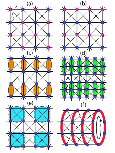
Figure 1: (color online) (a),(b) Néel and striped AFM phases used as magnetically ordered backgrounds in LSWT. Pink and blue bullets correspond to up and down arrangement of spins. (c),(d),(e),(f) Canditates of non-magnetic cluster orderings as a ground state background, used in COA. The case of (f) corresponds to string-VBS of $\ell=6$. Solid and dashed lines are $J_{1}$ and $J_{2}$ bonds, respectively.

In this paper, we therefore examine the spin-$\frac{1}{2}$ transverse field Ising model on the $J_{1}-J_{2}$ square lattice, Hamiltonian 1, by resorting to different analytical and numerical techniques such as linear spin-wave theory (LSWT) Henry et al. (2012), cluster operator approach (COA) Ganesh et al. (2013); Sadrzadeh, Marzieh and Langari, Abdollah (2015) and tree tensor network (TTN) simulation Verstraete et al. (2008). We found that harmonic quantum fluctuations in LSWT based on single-spin flip excitations are incapable of lifting the extensive degeneracy of the classical system. However, considering anharmonic fluctuations with multi-spin flip excitations via COA certifies the existence of global-loop-type of quantum fluctuations, which are able to lift the extensive degeneracy of the system at $J_{2}/J_{1}=0.5$ toward a string-VBS phase with broken lattice rotational symmetry, leading to an order by disorder transition. The string-VBS state is a manifestation of macroscopic quantum superposition Leggett (1980); Abad and Karimipour (2016). These findings are further confirmed by numerical (TTN) simulations.

The paper is organized as follows. In Sec. II, we introduce the model and some of its classical features. Next, in Sec. III we present LSWT and COA used for determining the true nature of quantum ground state by introducing different type of quantum fluctuations. We compare the results obtained from two approaches with each other and also with the TTN results. Details of our approaches are presented in Appendices. We argue that string-type quantum fluctuations can cast the ground state of highly frustrated point $J_{2}/J_{1}=0.5$ to a string-VBS phase at low fields with broken rotational symmetry. Sec. IV discusses the existence of a quantum phase transition from string-VBS phase of low fields to a quantum paramagnet phase of high fields at $\Gamma/J_{1}\cong 0.5$, where the critical exponents are extracted. Finally, the paper is summarized and concluded in Sec. V.

II Model

In this section, we introduce the spin-1/2 transverse field Ising model on the square lattice with $J_{1}-J_{2}$ interactions. We consider a square lattice, where spin-1/2 particles are placed at the vertices of the lattice and the antiferromagnetic exchange coupling $J_{1}$ ($J_{2}$) are tuned between the nearest neighbor (next-nearest neighbor) spins (see Fig. 1). Hamiltonian of the model in the presence of a transverse magnetic field $\Gamma$ is given by

$$\mathcal{H}=J_{1}\displaystyle\sum_{\langle i,j\rangle}{S_{i}^{z}S_{j}^{z}}+J_{2}\displaystyle\sum_{\langle\langle i,j\rangle\rangle}{S_{i}^{z}S_{j}^{z}}-\Gamma\displaystyle\sum_{i}{S_{i}^{x}},~{}$$ (1)

where ${S_{i}}\equiv(S_{i}^{x},S_{i}^{y},S_{i}^{z})$ are the usual quantum spin-1/2 operators with ${S_{i}}^{2}=S(S+1)$.

In the extreme case, where $J_{2}=0$ and $\Gamma=0$, the classical ground state of the system is given by a Néel state (Fig. 1-(a)), which persists as the frustration is increased up to a critical point at $J_{2}/J_{1}=0.5$, where it breaks to a collinear anti-ferromagnetic phase with striped AFM order (Fig. 1-(b)) for $J_{2}/J_{1}>0.5$, through a first-order quantum phase transition Oitmaa (1981); Morán-López et al. (1993); Kalz et al. (2009). The classical ground state of the system further displays an exponential degeneracy at the highly frustrated point $J_{2}/J_{1}=0.5$ in which the ground state is described by two-up-two-down configurations for spins on every crossed square of the lattice. Our aim in this paper is to study the effects of quantum fluctuations to lift this extensive degeneracy toward a unique quantum ground state. Hence, we consider $J_{2}/J_{1}=0.5$ with $\Gamma\neq 0$, which induces zero-point quantum fluctuations to the system due to $S^{x}$ that does not commute with other terms in the Hamiltonian 1.

III Nature of quantum fluctuations

III.1 Linear Spin Wave Theory

To incorporate harmonic quantum fluctuations within LSWT, we start with the degenerate classical magnetically ordered backgrounds at $J_{2}/J_{1}=0.5$, i.e. Néel and striped AFM phases shown in Fig. 1-(a, b). The transverse magnetic field, $\Gamma$, creates the same canting angle $\theta$ on each classical spin vector of the Néel and striped configurations. Accordingly, the classical spin components become $S^{x}_{i}=S\sin\theta$ and $S^{z}_{i}=\pm S\cos\theta$, where $\pm$ sign denotes up and down spins in the $z$-direction. The angle $\theta$ increases with the strength of the transverse field $\Gamma$ up to the maximum value of $\theta_{max}=\pi/2$ , which corresponds to a full polarization of the classical spins in the $+x$-direction for $\Gamma\geq\Gamma_{c}$, where $\Gamma_{c}$ is the critical magnetic field. For a system with $N$ spins, there are $2N$ bonds with $J_{1}$ coupling and 2N bonds with $J_{2}$ coupling on the square lattice. The classical ground state energy per spin for both the Néel and striped phases are therefore given as

$$\varepsilon_{cl}^{N\acute{e}el}=\varepsilon_{cl}^{striped}=-S^{2}cos^{2}\theta-\Gamma Ssin\theta.$$ (2)

After minimizing the classical energy per spin with respect to angle $\theta$, we set $\theta=\pi/2$ to obtain the critical transverse field $\Gamma_{c}^{LSWT}$, given by $\Gamma_{c}^{LSWT}=2S$. Then, a LSWT is constructed on each of the two classical canted Néel and canted striped AFM magnetically ordered backgrounds. Harmonic quantum fluctuations of LSWT around these classical reference states will reduce the magnitude of the classical order parameters and result in zero-point energy corrections. In a general formalism (see Appendix. A), we define $S_{l,p}$ as the p-th spin ($p=1,\ldots,n$) of the l-th cell, where $n$ is the number of spins in a magnetic unit cell. We consider small quantum fluctuations on the classical reference states by linearized Holstein-Primakoff transformations and finally obtain an effective diagonal quadratic form of Hamiltonian Eq. 1 as,

$$\mathcal{H}_{LSWT}=E_{cl}-\dfrac{N}{n}\displaystyle\sum_{p}{\left(\frac{\tilde{h}_{p}}{2}\right)}+\displaystyle\sum_{\textbf{k},p}{\omega_{\textbf{k},p}\left(c_{\textbf{k},p}^{\dagger}c_{\textbf{k},p}+\dfrac{1}{2}\right)},$$ (3)

where k sums over the first Brillouin zone of the lattice constructed from the centers of magnetic unit cells of the classical reference state. Furthermore, $p$ runs over the n spins of a magnetic unit cell, $\tilde{h}_{p}$ is a quantum correction and $\omega_{\textbf{k},p}$ define the spectrum of quasi-particles, which are created by the bosonic creation operators $c_{\textbf{k},p}^{\dagger}$. The effective Hamiltonian, Eq. 3, obtained within LSWT framework, shows that both Néel and striped magnetically ordered backgrounds have the same zero-point energy corrections, which is a result of the harmonic single-spin-flip excitations. Hence, quantum corrections at harmonic level do not distinguish between different ordered manifold of states, failing to lift the extensive degeneracy at $J_{2}/J_{1}=0.5$. Moreover, as shown in Fig. 5, we observe a violation of Hellmann-Feynman theorem at enough high fields before reaching the critical point $\Gamma_{c}^{LSWT}/J_{1}=1.0$. Indeed, by increasing the transverse field $\Gamma$, before reaching the critical value, the transverse magnetization obtained from Hellmann-Feynman theorem, $m_{x}=-\frac{1}{S}\frac{\partial\langle H\rangle}{\partial\Gamma}$, deviates from the expectation value of magnetic order parameter $m_{x}=\frac{1}{S}\langle S_{x}\rangle$, signaling a violation of the Hellmann-Feynman theorem. This inconsistency implies again that quantum fluctuations go beyond the harmonic level of approximation considered in LSWT.

III.2 Cluster Operator Approach

In order to consider anharmonic quantum fluctuations, we implement the cluster operator approach. Analogous to the spin-wave theory, a candidate cluster-ordered background is proposed above which, the anharmonic multi-spin excitations are defined. This is in contrast to the LSWT, where only single-spin excitations have been taken into account. Let us further note that COA besides the introduction of anharmonic quantum fluctuations, can reveal the existence of possible valence bond solid phases. Generally, VBS phases are appeared as a regular pattern of dimers, trimers, quadrumers or loops shown in Fig. 1-(c-f).

It is shown that at zero field and $J_{2}/J_{1}=0.5$, two-spin flip excitation on a dimer, three-spin flip excitation on a trimer or four-spin flip excitation on a quadrumer cost the same finite energy as a single-spin flip one, i.e. $4J_{1}$. This is true for any finite cluster, which is shown in Appendix. B. However, flipping the spins on a vertical or horizontal global closed loop costs zero excitation energy, keeping the system in the degenerate ground state manifold (see Appendix. B). Therefore, it can be anticipated that in the presence of quantum fluctuations by a transverse field $\Gamma$, such global loops are proper building blocks to construct the ground state structure of the model. To confirm such assertion, we consider four candidate cluster orderings shown in Fig. 1-(c-f) as ground state backgrounds used in COA. We obtain an effective theory by a bosonization formalism for each cluster configuration, and then compare their results with each other to confirm that the true excitations of the model are of the global-loop type, constructing a columnar string-VBS phase for low fields at the highly frustrated point.

The following steps are carried out to construct an effective theory for the candidate cluster ordered backgrounds of Fig. 1. First, we rewrite the Hamiltonian, Eq. 1, as a sum over two terms, $\mathcal{H}=\mathcal{H}_{0}+\mathcal{H}_{int}$, where $\mathcal{H}_{0}=\sum_{I}{\mathcal{H}}_{I}$ denotes the set of shaded isolated clusters and $\mathcal{H}_{int}$ defines the interaction Hamiltonian between them. Next, we associate a boson to each eigenstate of the TFI Hamiltonian on a single cluster. In this respect, each eigenstate $|u\rangle$ of cluster I is created by a boson creation operator $b_{I,u}^{\dagger}$ acting on the vaccum $|0\rangle$, i.e. $|u\rangle_{I}=b_{I,u}^{\dagger}|0\rangle$, where $b_{I,u}^{\dagger}$ and $b_{I,u}$ are usual bosonic operators, satisfying $[b_{I,u},b_{I,u}^{\dagger}]=1$ and $[b_{I,u}^{(\dagger)},b_{I,u}^{(\dagger)}]=0$. Hence, a cluster ordered background is a Bose-condensate of ground state $|u=1\rangle$ bosons, i.e.

$$\langle b_{I,1}^{\dagger}b_{I,1}\rangle\equiv\bar{p}^{2},\quad\forall I$$ (4)

where $\bar{p}$ is the condensation amplitude and $\bar{p}^{2}$ gives the probability of such condensation. In the absence of inter-cluster interactions, $\bar{p}^{2}$ is equal to unity. Therefore, the Bose-condesate background acts like an ordered-reference state, above which quantum fluctuations will reduce the magnitude of condensation probability $\bar{p}^{2}$ and result in zero-point energy corrections. In other words, inter-cluster interactions give rise to low-lying excitations above the perfect cluster ordered background. As a result of hybridization of ground state of each cluster to other excited states, the value of $\bar{p}^{2}$ reduces from unity by bringing about a non-zero occupation of other excited bosons. Nevertheless, for preserving the Hilbert space of the effective model, the total occupation of bosons per cluster should be equal to one. According to these arguments, the effective Hamiltonian for a cluster ordered background can now be written in a quadratic bosonic form within a mean-field approximation of condensated bosons, as

$$\mathcal{H} = N_{c}\bar{p}^{2}\epsilon_{1}+\sum_{I}\sum_{u}\epsilon_{u}b_{I,u}^{\dagger}b_{I,u}$$

$$-\mu\Big{[}N_{c}\bar{p}^{2}+\sum_{I,u\neq 1}b_{I,u}^{\dagger}b_{I,u}-N_{c}\Big{]}$$

$$+\bar{p}^{2}\sum_{\langle I,J\rangle}\sum_{u,v}\Big{[}(d_{uv}^{IJ})\>b_{I,u}^{\dagger}b_{J,v}^{\dagger}+(h_{uv}^{IJ})\>b_{I,u}^{\dagger}b_{J,v}+h.c.\Big{]}.$$

The first line includes intra-cluster terms, where the index $I$ sums over all isolated clusters, $u$ sums over the dominant excited states of each cluster with corresponding eigen energies $\epsilon_{u}$, and $N_{c}$ denotes the total number of isolated clusters. The second line enforces single boson occupancy constraint, via a chemical potential $\mu$. The third line involves inter-cluster terms, where $u,v$ are the two excited bosons of neighboring clusters $I$ and $J$, respectively. Coefficients $d_{uv}^{IJ}=\langle uv|\mathcal{H}_{IJ}|11\rangle$ and $h_{uv}^{IJ}=\langle u1|\mathcal{H}_{IJ}|1v\rangle$ are respectively creation and hopping amplitudes between excited bosons of neiboring clusters. The minimization of ground-state energy of the bosonic effective theory in addition to the conservation of Hilbert space dimension are satisfied by the solution of $\frac{\partial\langle\mathcal{H}\rangle}{\partial\mu}=0$ and $\frac{\partial\langle\mathcal{H}\rangle}{\partial\bar{p}}=0$ equations. Details of the bosonic effective theory for COA are given in Appendix. C.

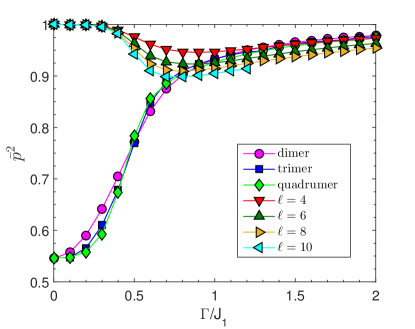
Figure 2: (color online) The condensation probability $\bar{p}^{2}$ for different cluster orderedings of Fig. 1-(c, d, e, f). $\ell$ denotes the cylinder perimeter length considered in COA for a string-ordered background shown in Fig. 1-(f)

The condensation probability $\bar{p}^{2}$ of different cluster orderings shown in Fig. 1-(c, d, e, f) is demonstrated in Fig. 2. We found that for low transverse fields ($\Gamma<0.5$), there is a strong condensation probability (near unity) of the global loops ($\ell=4,6,8,10$) on the lattice, while the condensation probability of dimers, trimers and plaquettes (quadrumers) is weak ($\sim 0.55$). We have also considered the staggered dimer configuration in our calculations not shown here, which gives a result similar to the dimer case. Let us note that a global loop is a closed string, which covers all sites along a horizontal or vertical direction of the periodic square lattice, as shown in Fig. 1-(f). This implies that at low fields the proper conjecture for the ground-state structure is based on the global loops, while finite size clusters fail to condensate properly in the ground state.

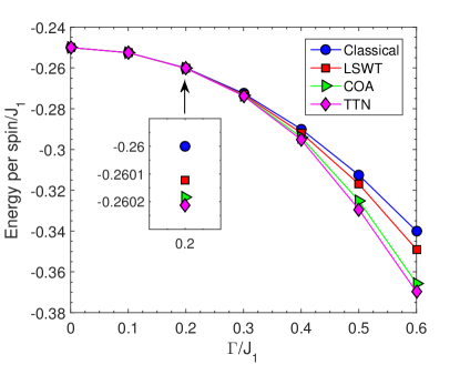
Figure 3: (color online) Ground-state energy per site versus transverse magnetic field. A comparision between classical, linear-spin wave, cluster operator (with string-ordered background on $\ell=10$ cylinder) and tree-tensor network (on a 8 $\times$ 6 lattice) approaches is presented. The inset shows the magnified data for $\Gamma/J_{1}=0.2$.

The results of Fig. 2 suggest a string-VBS phase for the ground state of our model at low fields. It turns out that anharmonic quantum fluctuations, mediated in terms of COA, lift the classical degeneracy at the highly frustrated point, towards a string-VBS phase, which breaks lattice rotational symmetry and leaves the system with a two-fold degenerate ground state. The ground-state energy per site versus transverse magnetic field is illustrated in Fig. 3. We observe that the energy of the string-VBS state obtained from COA is less than the classical and LSWT ones, justifying the existence of string formation in the ground state. The inset of Fig. 3 clearly shows the lower energy value of COA for a low field value $\Gamma/J_{1}=0.2$. We have also shown the ground-state energy obtained from TTN numerical algorithm, as a reference close to the exact diagonalization data. The numerical TTN is a renormalization ansatz to simulate large lattice sizes that is explained in Appendix. D. Accuracy of our data on $\{4\times 6,\,6\times 6,\,6\times 8\}$ lattices is of order, respectively, $\{10^{-8},\,10^{-5},\,10^{-4}\}$ which is not presented here.

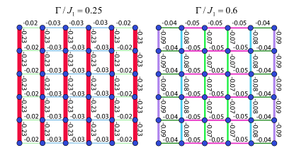
Figure 4: (color online) Nearest-neighbor correlations, $C_{NN}$, obtaind by TTN numerical simulation, which measures the breaking of lattice rotational symmetry in the string-VBS phase. Left panel: low-field regime representing the string-VBS state. Right panel: high-field regime of the quantum paramagentic phase, which preserves rotational symmetry.

The nature of ground state can be represented by the nearest-neighbor (NN) correlation function,

$$C_{NN}=\langle S_{i}^{z}S_{j}^{z}\rangle,\;\;\;i,j:\mbox{NN on the lattice}.$$ (6)

In this respect, we compute $C_{NN}$ on a 6$\times$6 lattice using TTN which is shown in Fig. 4, for two different values of transverse field $\Gamma$. The left panel of Fig. 4 corresponds to low-field regime ($\Gamma/J_{1}=0.25$), while the right panel corresponds to the high-field values ($\Gamma/J_{1}=0.60$). The left panel shows that the correlations along the vertical direction are close to their maximum value of Néel type ordering ($|C_{NN}^{max}|=0.25$), while the correlations on the horizontal direction is very small. This is a clear signature of the string formation as a VBS phase. The emergence of strings could be either in vertical or horizontal direction, breaking the rotational symmetry of the lattice which manifests the two-fold degeneracy. Increasing the magnetic field to the high-field regime drives the model to a quantum paramagnet, which has rotational symmetry and leads to almost equal correlations along the two perpendicular directions as shown in the right panel of Fig. 4. Such symmetry breaking of ground state at low fields is a signature for presence of a quantum phase transition from the string-VBS phase of low fields to the quantum paramagentic phase of high fields, which is investigated with more details in the next section.

IV Quantum phase transition

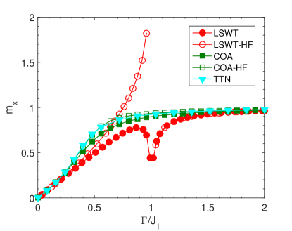
Figure 5: (color online) Transverse magnetization calculated by different methods, LSWT, COA and TTN. The value obtained directly from the expectation value of $S_{x}$ operator, $m_{x}=\frac{1}{S}\langle S^{x}\rangle$ is compared with the one obtained from Hellmann-Feynmann theorem, $m_{x}^{HF}=-\frac{1}{S}\frac{\partial\langle H\rangle}{\partial\Gamma}$.

In this section, we study the behavior of field induced magnetization, $m_{x}=\frac{1}{S}\langle S^{x}\rangle$, by increasing the transverse field from the low-field to high-field regimes. The magnetization as a function of transverse field calculated by different approaches is depicted in Fig. 5. Moreover, the transverse magnetization $m_{x}$, obtained directly from the expectation value of $S_{x}$ operator, is compared with the derivative of effective Hamiltonian expectation value versus $\Gamma$, i.e. $m_{x}^{HF}=-\frac{1}{S}\partial\langle H\rangle/\partial\Gamma$ corresponding to Hellmann-Feynmann theorem. As we mentioned in Sec. III.1, LSWT exhibits a violation of the Hellmann-Feynmann theorem as the magnetic field increases toward the high-field regime. This implies that when increasing the transverse field Γ, quantum fluctuations are beyond the harmonic level of approximation considered in LSWT. However, COA results are in a good agreement with the Hellmann-Feynmann theorem and numerical results obtained from TTN simulation. The COA results further show that the anharmonic quantum fluctuations will render the violated region of the Hellmann-Feynmann theorem to the quantum paramagnet phase, proposing a lower critical value than the LSWT counterpart, between the string-VBS and quantum paramagnet phases.

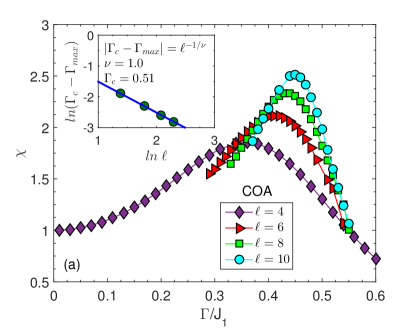
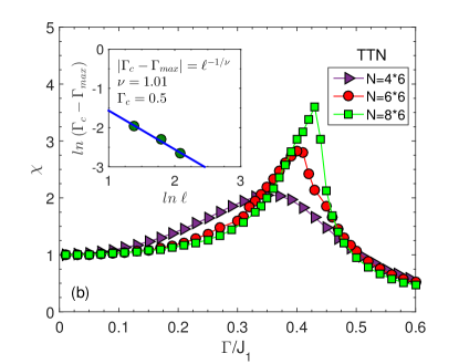
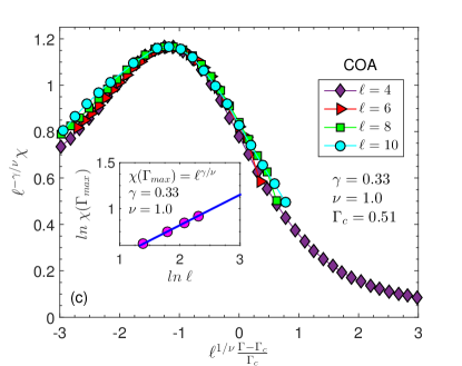
Figure 6: (color online) (a), (b) Magnetic susceptibility obtained from COA and TTN, respectively for different system sizes. They show a sharp peak indicating a phase transition from string-VBS phase of low fields to the quntum paramagnet of high fields, at $({\Gamma/J_{1}})_{c}=0.5\pm 0.01$ with exponent $\nu=1.0\pm 0.01$. (c) Data collapse of magnetic susceptibility obtained from COA, which shows the scale invariance of susceptibility governed by exponent $\gamma=0.33\pm 0.01$.

Quantum phase transition can be traced out by the divergent behavior of magnetic susceptibility, which is the derivative of transverse magnetization with respect to the magnetic field,

$$\chi=\frac{\partial m_{x}}{\partial\Gamma}=-\frac{1}{S}\frac{\partial^{2}E}{\partial\Gamma^{2}}.$$ (7)

The magnetic susceptibility of COA data is plotted in Fig. 6-(a), which shows sharper and stronger divergence as the length ($\ell$) of lattice is increased. Let us note that the COA results with string-ordered background are obtained for lattices defined on an infinite cylinder that has a finite perimeter length $\ell$. Finite-size scaling theory tells us how to estimate the critical exponents for the model Nishimori and Ortiz (2011). The divergent behavior of $\chi$ obeys the following scaling relations

$$|\Gamma_{c}-\Gamma_{max}| \sim \ell^{-1/\nu},$$ (8)

$$\chi(\Gamma_{max}) \sim \ell^{\gamma/\nu},$$ (9)

where $\Gamma_{c}$ is the critical field in the thermodynamic limit, $\Gamma_{max}$ is the position of maximum of finite-lattice susceptibility $\chi$, $\nu$ is the correlation length exponent i.e. $\xi\sim|\Gamma-\Gamma_{c}|^{-\nu}$ and $\gamma$ is an exponent, which governs singularity in the magnetic susceptibility. As shown in the inset of Fig. 6-(a), we find a good scaling for COA data, which gives $\nu=1.0\pm 0.01$ and $\Gamma_{c}=0.51\pm 0.01$. A similar behavior is also observed for $\chi$ versus $\Gamma$ of the TTN numerical computation presented in Fig. 6-(b). Accordingly, the same critical field and exponent $\nu$ are also reported in the inset of Fig. 6-(b). Once we have obtained $\nu$ and $\Gamma_{c}$ from Eq. 8, we can use them to find $\gamma$ from Eq. 9, as well as getting the scale invariant behavior of magnetic susceptibility, which is observed from a good data collapse of different sizes in Fig. 6-(c). It shows the scale invariance of susceptibility with exponent $\gamma=0.33\pm 0.01$. Both COA and TTN imply a continuous phase transition from string-VBS phase (at low fields) to the quantum paramagnet phase (at high fields) at $\Gamma_{c}=0.5\pm 0.01$. The continuous nature of such transition is confirmed by the broken lattice rotational symmetry in the string-VBS phase compared with symmetric quantum paramagnet phase.

We would like to comment on the nature of string-VBS ground state. The formation of loops yields the ground state to inherit partially the one-dimensional (1D) character of TFI model. At zero field, the ground state of 1D TFI model is doubly degenerate, which is given by classical antiferromagnetic state $|\phi\rangle=|+-+-\dots+-\rangle$ and its spin flipped one $|\bar{\phi}\rangle=|-+-+\dots-+\rangle$, where $|+\rangle,|-\rangle$ represent the eigenstates of $S^{z}$ Pauli operator. In the presence of small transverse field, the ground state is a linear superposition of different configurations mostly occupied by $|\phi\rangle$ and $|\bar{\phi}\rangle$. This is actually a macroscopic superposition of quantum states, which has been discussed by Leggett Leggett (1980) to distinguish between macroscopic quantum superposition and quantum entangelement. A recent study in Ref. Abad and Karimipour (2016) verifies that the ground state of 1D TFI model in AFM region is essentially a superposition of the two macroscopic distinct states $|\phi\rangle$ and $|\bar{\phi}\rangle$, i.e. a macroscopic quantum superposition. We therefore conjuncture that the string-VBS state is a witness for two-dimensional version of macroscopic quantum superposition. In other words, we conclude that string-VBS phase consists of a columnar ordering of string-valence bonds each of which in an equal superposition of two possible Néel configurations with no magnetic order in z-direction.

V Summary and Conclusions

We have studied the zero-temperature phase diagram of the transverse field Ising model on the $J_{1}-J_{2}$ square lattice at the highly frustrated point $J_{2}/J_{1}=0.5$, which is known to have an extensive degenerate classical ground state at $\Gamma=0$. The LSWT analysis of the model failed to lift this classical degeneracy implying that harmonic fluctuations, coming from the single-spin flip excitations, are not able to represent the true quantum fluctuations of the system at the highly frustrated region. We therefore, applied the cluster operator approach, which is based on the multi-spin flip type of anharmonic quantum fluctuations above a non-magnetic cluster ordered background. We found that the exponential degeneracy of the classical ground state at $J_{2}/J_{1}=0.5$ is lifted toward a string-VBS phase which breaks rotational symmetry of the lattice with only two-fold degeneracy. This is a manifestation of order-by-disorder transition that is induced by anharmonic quantum fluctuations.

The quantum phase transition between string-VBS phase at low fields and quantum paramagnet phase at high fields occurs at the critical point $(\Gamma/J_{1})_{c}=0.50\pm 0.01$ and is of a continuous type as the rotational symmetry is only broken at the string-VBS phase. The critical exponents have been obtained to be $\nu=1.0\pm 0.01$ and $\gamma=0.33\pm 0.01$. Moreover, we conjuncture that the string-VBS state is an example of macroscopic superposition of distinct quantum states in 2D, where the whole lattice is a direct product of 1D ground states, i.e. $\bigotimes_{j}\big{(}|\phi_{j}\rangle+|\bar{\phi}_{j}\rangle\big{)}$.

Let us discuss the connection of our results to the phase diagram of spin-1/2 $J_{1}-J_{2}$ AFM Heisenberg model on two-dimensional square lattice. The ground state structure of Heisenberg model at $J_{2}/J_{1}=0.5$ is controversial to be either a valence bond solid state or a spin liquid phase Singh et al. (1999); Metavitsiadis et al. (2014); Isaev et al. (2009); Yu and Kao (2012); Doretto (2014); Hu et al. (2013); Wang et al. (2013); Gong et al. (2014); Morita et al. (2015); Jiang et al. (2012); Mezzacapo (2012); Li et al. (2012); Ren et al. (2014). Early studies proposed that anharmonic fluctuations could make a dimer-VBS Chubukov and Jolicoeur (1991) or a plaquatte-VBS Zhitomirsky and Ueda (1996) as stable phases around $J_{2}/J_{1}=0.5$, granting that short-range corrections to the ground-state energy are small. Our COA results on TFI model with dimer-VBS is similar to the case of Ref.Chubukov and Jolicoeur (1991), where dimer-VBS corrections are not small to construct a stabilized dimer-VBS at $J_{2}/J_{1}=0.5$. According to the recent investigations, a quntum spin liquid is more plausible phase for the intermediate region of the Heisenberg model Hu et al. (2013); Wang et al. (2013); Gong et al. (2014); Morita et al. (2015); Jiang et al. (2012); Mezzacapo (2012); Li et al. (2012); Ren et al. (2014). On the other hand, our results on TFI model govern the high anisotropy limit of the Heisenberg model, where the easy-axis coupling is much stronger than the coupling in the fluctuating plane. It suggests that we get the string-VBS ground state by increasing the easy-axis anisotropy of the Heisenberg model. In other words, we conclude that by reduction of symmetry from $SU(2)$ to $Z_{2}$, plausible spin liquid phase of $J_{1}-J_{2}$ Heisenberg model on the square lattice cast to a string-VBS phase at the highly frustrated point $J_{2}/J_{1}=0.5$. Such a novel string-VBS phase can also emerge in the case of reducing quantum fluctuations by increasing the dimensionality or the spin quantum number, as it was predicted in previous literature for a $S=1$ $J_{1}-J_{2}$ Heisenberg model on the square lattice Cai et al. (2007); Jiang et al. (2009).

VI Acknowledgements

S.S.J. and A.L. acknowledge support from the Iran National Science Foundation under Grant No. 93023859 and Sharif University of Technology’s Office of Vice President for Research.

Appendix A Linear Spin Wave Theory

We use the three classical reference states shown in Fig. 7 as a background on which harmonic spin waves are considered. Magnetic unit cell of each background state is shown with a red rectangle in Fig. 7. As a general formalism Henry et al. (2012), we define $S_{l,p}$ as the p-th spin ($p=1,\ldots,n$) of the l-th cell, where $n$ is the number of spins in a magnetic unit cell. In the classical limit, an applied transverse field $\Gamma$ rotates all spins around the $y$ axis by an angle $\theta$. We now introduce a local rotation of spins, as $S_{l,p}\rightarrow\tilde{S}_{l,p}$, in such a way that all three classical states shown in Fig.7 map to a simple ferromagnetic state in $z$ direction, i.e. $\tilde{S}^{z}_{l,p}=S$ everywhere. Accordingly, we define

$$\tilde{S}_{l,p}=\sigma_{p}R_{y}(\sigma_{p}\theta)S_{l,p}$$ (10)

where $\sigma_{p}=\pm 1$ denotes the direction of p-th spin along the $z$ axis, and $R$ is the rotation matrix around $y$ axis by an angle $\sigma_{p}\theta$. Therefore, the following relations between spin components in the rotated and non-rotated representations are obtained

$$S^{z}_{l,p}=\sigma_{p}cos\theta\tilde{S}^{z}_{l,p}-sin\theta\tilde{S}^{x}_{l,p},$$

$$S^{x}_{l,p}=\sigma_{p}cos\theta\tilde{S}^{x}_{l,p}+sin\theta\tilde{S}^{z}_{l,p}.$$ (11)

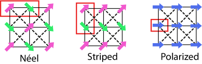
Figure 7: (color online) Schematic representations of the classical magnetically ordered states around which we consider harmonic quantum fluctuations of LSWT. Magnetic unit cells of each classical phase are shown with red rectangles.

After rewriting the Hamiltonian in terms of new spin operators $\tilde{S}^{z}_{l,p}$ and $\tilde{S}^{x}_{l,p}$, we consider small quantum fluctuations around this general ferromagnetic classical reference state by the following linearized Holstein-Primakoff transformations,

$$\tilde{S}^{z}_{l,p}=S-a_{l,p}^{\dagger}a_{l,p},\quad\tilde{S}^{x}_{l,p}\approx\sqrt{\dfrac{S}{2}}\left(a_{l,p}^{\dagger}+a_{l,p}\right),$$ (12)

where $a_{l,p}$ and $a_{l,p}^{\dagger}$ are bosonic operators with well-known commutation relations $[a_{l,p},a_{l,p}^{\dagger}]=1$ and $[a_{l,p}^{(\dagger)},a_{l,p}^{(\dagger)}]=0$. Hamiltonian is expanded up to the quadratic order of bosonic operators,

$$\mathcal{H}_{LSWT} =E_{cl}+\displaystyle\sum_{l,p}{\tilde{h}_{p}a^{\dagger}_{lp}a_{lp}}$$ (13)

$$+\dfrac{1}{8} \sin^{2}\theta\displaystyle\sum_{l,{\bm{\delta}},p,p^{\prime}}{\tilde{J}({\bm{\delta}})_{pp^{\prime}}\left(a^{\dagger}_{l,p}+a_{l,p}\right)\left(a^{\dagger}_{l^{\prime},p^{\prime}}+a_{l^{\prime},p^{\prime}}\right)},$$

where linear terms vanish by construction and $\tilde{J}({\bm{\delta}})$ is an $n\times n$ matrix, containing the couplings between spins $p,p^{\prime}$ of the two unit cells $l,l^{\prime}$ at position ${\bm{\delta}}$ and

$$\tilde{h}_{p} = -\frac{1}{2}\sigma_{p}\cos^{2}(\theta)\displaystyle\sum_{{\bm{\delta}},p^{\prime}}\left[\tilde{J}({\bm{\delta}})\right]_{pp^{\prime}}\sigma_{p^{\prime}}+\Gamma\sin\theta.$$ (14)

The momentum space representation is used with the following transformations,

$$a_{{\bm{k}},p} = \sqrt{\dfrac{n}{N}}\displaystyle\sum_{l}{e^{\mathrm{i}{\bm{k}}.{\bm{r}}_{l}}a_{l,p}},$$

$$\tilde{J}(\bm{k}) = \displaystyle\sum_{\bm{\delta}}{e^{-\mathrm{i}{\bm{k}}.{\bm{\delta}}}\tilde{J}(\bm{\delta})}~{}.$$ (15)

Hence, the quadratic Hamiltonian can be written in the following compact form

$$\mathcal{H}_{LSWT} = E_{cl}-\dfrac{N}{n}\displaystyle\sum_{p}{\left(\frac{\tilde{h}_{p}}{2}\right)}+\dfrac{1}{2}\displaystyle\sum_{\bm{k}}{A_{\bm{k}}^{\dagger}M_{\bm{k}}A_{\bm{k}}},$$

where

$$A_{\bm{k}}^{\dagger} = (a_{{\bm{k}},1}^{\dagger},\ldots,a_{{\bm{k}},n}^{\dagger},a_{-{\bm{k}},1},\ldots,a_{-{\bm{k}},n}),$$

$$M_{\bm{k}} = \begin{pmatrix}\tilde{h}+\Delta_{\bm{k}}&\Delta_{\bm{k}}\\ \Delta_{\bm{k}}&\tilde{h}+\Delta_{\bm{k}}\end{pmatrix},$$

$$[\tilde{h}]_{pp^{\prime}} = \tilde{h}_{p}\delta_{pp^{\prime}},$$

$$\Delta_{\bm{k}} = \dfrac{1}{2}\left(\tilde{J}(\bm{k})+\tilde{J}(-\bm{k})\right).$$ (17)

Finally, performing an n-mode paraunitary Bogoliubov transformation Colpa (1978), we obtain the effective diagonal quadratic Hamiltonian given by

$$\mathcal{H}_{LSWT}=E_{cl}-\dfrac{N}{n}\displaystyle\sum_{p}{\left(\frac{\tilde{h}_{p}}{2}\right)}+\displaystyle\sum_{\textbf{k},p}{\omega_{\textbf{k},p}\left(c_{\textbf{k},p}^{\dagger}c_{\textbf{k},p}+\dfrac{1}{2}\right)},$$ (18)

where k sums over the first Brillouin zone of a lattice constructed from the centers of magnetic unit cells of the classical reference states and $p$ runs over the spins of a magnetic unit cell, $\tilde{h}_{p}$ is a correction term gained from bosonic commutation relations and $\omega_{\textbf{k},p}$ defines the spectrum of quasi-particles with corresponding bosonic creation operators $c_{\textbf{k},p}^{\dagger}$. In fact, the eigenmodes $\omega_{\textbf{k},p}$ are the eigenvalues of $\Xi M_{\bm{k}}$, where $\Xi$ matrix is given by

$$\Xi=\begin{pmatrix}I_{n}&0_{n}\\ 0_{n}&-I_{n}\end{pmatrix}~{}.$$ (19)

Finally, the eigenmodes $\omega_{\textbf{k},p}$ can be expressed in terms of the eigenvalues $\lambda_{\textbf{k},p}$ of matrix $\Delta_{\bm{k}}$ in the form

$$\omega_{\textbf{k},p}=\tilde{h}_{p}\sqrt{1+2\frac{\lambda_{\textbf{k},p}}{\tilde{h}_{p}}}.$$ (20)

Appendix B Excited states in zero field

At the highly frustrated point $J_{2}/J_{1}=0.5$ and zero transverse field, the ground state of Hamiltonian Eq. 1 is highly degenerate. A typical state of this ground space is the Néel state shown in Fig. 8. The lowest-energy excitations might be either a single-spin flip or a joint flip of all spins of a specific cluster, which are shown in Fig. 8. In a Néel configuration all nearest-neighbor bonds $J_{1}$ are satisfied, while the next-nearest neighbor bonds $J_{2}$ are not. Accordingly, flipping one spin will satisfy four $J_{2}$-bonds, while dissatisfy four $J_{1}$-bonds. Hence, the energy cost of a single-spin flip excitation is given by $8(J_{1}-J_{2})$, which is equal to $4J_{1}$ at $J_{2}/J_{1}=0.5$. Similarly, the energy cost of a dimer-flip, trimer-flip, plaquette flip or every finite cluster flip will be $4J_{1}$. However, a joint flip of all spins on a global loop of the lattice (green loop in Fig. 8) costs $4n(J_{1}-2J_{2})$, where $n$ is the number of spins on the global loop. Therefore, it implies a zero energy cost at $J_{2}/J_{1}=0.5$, which corresponds to the transformation of Néel state to another state of the highly degenerate manifold. Therefore, the energy cost of a global loop flip is lower than any other finite cluster flip, at the highly frustrated point $J_{2}/J_{1}=0.5$.

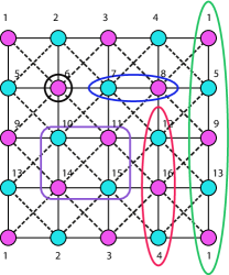
Figure 8: (color online) A classical Néel configuration of Hamiltonian 1 at zero field, with periodic boundary conditions on both sides. All $J_{1}$ bonds are satisfied with this phase while it is not the case for $J_{2}$ bonds. Different kinds of spin excitations corresponding to single-spin flip, dimer-flip, trimer-flip, plaquette-flip and global-loop flip are shown.

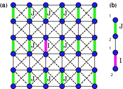
Figure 9: (color online) (a) A columnar ordering of dimers as a ground state background, used in COA. (b) The interaction between two ‘nearest-neighbor’ dimers $I$ and $J$, given by $J_{1}S_{1(I)}^{z}S_{2(J)}^{z}$.

Appendix C Cluster Operator Approach

In cluster operator approach (COA), we first consider a perfect multi-spin cluster ordering as a ground state background, in which all isolated clusters are in their unique ground states. Quantum fluctuations by inter-cluster interactions around such ordered reference state give rise to low-lying excitations above the perfect cluster ordered background, as a result of hybridization of ground state of each cluster to its other excited states, which eventuate the zero-point energy correction. In the following, we first propose two-spin clusters with columnar orderings shown in Fig. 9-(a). The method for other cluster ordered backgrounds will be similar to this.

In order to construct an effective theory for the dimer ordered background, we rewrite the Hamiltonian 1 as $\mathcal{H}=\mathcal{H}_{0}+\mathcal{H}_{int}$, where $\mathcal{H}_{0}=\sum_{C}{\mathcal{H}}_{C}$ denotes the set of shaded isolated dimers shown in Fig. 9 and $\mathcal{H}_{int}$ defines the interaction between them.

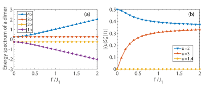
Figure 10: (color online) (a) Energy spectrum (in units of $J_{1}$) of a single dimer versus $\Gamma/J_{1}$. The bottom line ($|1\rangle$) is the unique ground state of the dimer. (b) Transition amplitude $\langle u|S_{\alpha}^{z}|1\rangle$ ($\alpha=1,2$), between the ground state $|1\rangle$ and four eigenstates $|u\rangle$ of a dimer, versus transverse field $\Gamma/J_{1}$.

The Hamiltonian of a single dimer is given by

$$\mathcal{H}_{single-dimer} = J_{1}(S_{1}^{z}S_{2}^{z})-\Gamma(S_{1}^{x}+S_{2}^{x}).$$ (21)

The dimer Hamiltonian is diagonalized exactly. The energy spectrum as a function of $\Gamma/J_{1}$ is shown in Fig. 10-(a). It shows a unique ground state $|1\rangle$ at non-zero transverse field $\Gamma$. In order to develop an effective theory including inter-dimer interactions $\mathcal{H}_{int}$, we first examine the interaction between two neighboring dimers. Accordingly, we deduce which excited states of each dimer participate in the dynamics of the system when imposing quantum fluctuations above the perfect columnar dimer ordered background. Fig. 9-(a) shows that each dimer $I$ interacts with eight neighboring dimers $J$. Let us consider interaction between two dimers $I$ and $J$, via a bond $J_{1}$ between spin 1 of dimer $I$ and spin 2 of dimer $J$, shown in the Fig. 9-(b). The interaction, $\mathcal{H}_{IJ}$, is given by

$$\mathcal{H}_{IJ}=J_{1}S_{1(I)}^{z}S_{2(J)}^{z}.$$ (22)

In the absence of this interaction, both dimers I and J are in their unique ground states $|1\rangle$. Thus, the state of two-dimer system is $|11\rangle$, i.e. a direct product of single-dimer ground states. Now we proceed to turn on the interaction term $\mathcal{H}_{IJ}$ between two dimers, as a perturbation. $\mathcal{H}_{IJ}$ does not commute with the isolated dimer Hamiltonian, Eq. 21, which hybridizes the ground state of each dimer with its excited states. Accordingly, the matrix elements of $\mathcal{H}_{IJ}$ between two direct product states, $|uv\rangle$ and $|11\rangle$, are given by

$$\langle uv|\mathcal{H}_{IJ}|11\rangle=J_{1}\langle u|S_{1(I)}^{z}|1\rangle\times\langle v|S_{2(J)}^{z}|1\rangle,$$ (23)

where $|u\rangle$ and $|v\rangle$ are four possible eigenstates of dimers I and J, respectively. Fig. 10-(b) represents the behavior of transition amplitude $\langle u|S_{\alpha}^{z}|1\rangle$ ($\alpha=1,2$), between the ground state $|1\rangle$ and four eigenstates $|u\rangle$ of a single dimer. It shows clearly that for all values of $\Gamma/J_{1}$, there are two excited states $u=2,3$ which dominantly contribute to the dynamics of the system as quantum fluctuations. Accordingly, in the following section we construct an effective theory for the columnar dimer ordered background via a bosonization formalism including only three eigenstates $|u\rangle$ $(u=1,2,3)$ of each dimer.

We introduce a bosonization formalism (Sachdev and Bhatt, 1990), similar to what has been done in Ref. Ganesh et al., 2013; Sadrzadeh, Marzieh and Langari, Abdollah, 2015 to obtain the effective theory. We associate a boson to each of the three eigenstates $|u\rangle$ of each dimer $(u=1,2,3)$. In this respect, each eigenstate $|u\rangle$ of dimer $I$ is created by a boson creation operator $b_{I,u}^{\dagger}$ acting on the vaccum $|0\rangle$,

$$|u\rangle_{I}=b_{I,u}^{\dagger}|0\rangle,\ u=1,2,3$$ (24)

where $b_{I,u}^{\dagger}$ and $b_{I,u}$ are usual bosonic operators, satisfying $[b_{I,u},b_{I,u}^{\dagger}]=1$ and $[b_{I,u}^{(\dagger)},b_{I,u}^{(\dagger)}]=0$. According to the earlier definition, columnar dimer ordered background is a Bose-condensate of ground state $|u=1\rangle$ bosons, i.e. at a mean field level we write

$$b_{I,1}\equiv b_{I,1}^{\dagger}\equiv\bar{p},\quad\forall I$$ (25)

where $\bar{p}$ is the condensation amplitude and $\bar{p}^{2}$ gives the probability of a single dimer to be in its ground state. In the absence of interaction between dimers, $\bar{p}^{2}$ is equal to unity. However, the existence of inter-dimer interactions reduce $\bar{p}^{2}$ from unity, giving rise to a non-zero occupation of excited bosons on single dimers. Nevertheless, to preserve the Hilbert space of the effective model, the total occupancy of bosons per dimer should be unity, i.e.

$$N_{d}\bar{p}^{2}+\displaystyle\sum_{I,u=2,3}{b_{I,u}^{\dagger}b_{I,u}}=N_{d},$$ (26)

where $N_{d}$ is the total number of dimers in Fig. 9-(a). Having in mind the Bose-condensation of ground bosons, the excited bosons are present in very dilute concentrations, which lead to neglect the interaction between excited bosons. Hence, we only consider the interactions between excited bosons and ground bosons. In the bosonic language, there are two kinds of inter-dimer interactions participating in the effective Hamiltonian. First, a creation (annihilation) term of excited bosons on neighboring dimers,

$$|uv\rangle\langle uv|\mathcal{H}_{IJ}|11\rangle\langle 11| \equiv d_{uv}^{IJ}\>\bar{p}^{2}\>b_{I,u}^{\dagger}b_{J,v}^{\dagger}\,,$$

$$|11\rangle\langle 11|\mathcal{H}_{IJ}|uv\rangle\langle uv| \equiv {d_{uv}^{IJ}}^{\dagger}\>\bar{p}^{2}\>b_{I,u}b_{J,v}\,,$$ (27)

and second, a hopping term of excited bosons between neighboring dimers,

$$|u1\rangle\langle u1|\mathcal{H}_{IJ}|1v\rangle\langle 1v| \equiv h_{uv}^{IJ}\>\bar{p}^{2}\>b_{I,u}^{\dagger}b_{J,v}\,,$$

$$|1v\rangle\langle 1v|\mathcal{H}_{IJ}|u1\rangle\langle u1| \equiv {h_{uv}^{IJ}}^{\dagger}\>\bar{p}^{2}\>b_{I,u}b_{J,v}^{\dagger}\,,$$ (28)

where coefficients $d_{uv}^{IJ}=\langle uv|\mathcal{H}_{IJ}|11\rangle$ and $h_{uv}^{IJ}=\langle u1|\mathcal{H}_{IJ}|1v\rangle$ are creation and hopping amplitudes, respectively. On the other hand, according to Fig. 10-(b), the values of terms like $\langle 1|S_{\alpha}^{z}|1\rangle$ are zero, which rules out $\mathcal{O}(\bar{p}^{3})$ and $\mathcal{O}(\bar{p}^{4})$ terms in the effective Hamiltonian. Those terms independent of $\bar{p}$ and $\mathcal{O}(\bar{p})$ can be ignored due to neglecting interaction between excited bosons.

Based on the above arguments, the effective Hamiltonian for the columnar dimer ordered background can now be written in a quadratic bosonic form,

$$\mathcal{H} = N_{d}\bar{p}^{2}\epsilon_{1}+\sum_{I}\sum_{u}\epsilon_{u}b_{I,u}^{\dagger}b_{I,u}$$

$$-\mu\Big{[}N_{d}\bar{p}^{2}+\sum_{I,u}b_{I,u}^{\dagger}b_{I,u}-N_{d}\Big{]}$$

$$+\bar{p}^{2}\sum_{\langle I,J\rangle}\sum_{u,v}\Big{[}(d_{uv}^{IJ})\>b_{I,u}^{\dagger}b_{J,v}^{\dagger}+(h_{uv}^{IJ})\>b_{I,u}^{\dagger}b_{J,v}+H.c.\Big{]}.$$

The first line includes intra-dimer terms, where the index $I$ sums over all isolated dimers in Fig. 9-(a) and $u$ sums over the two dominant excited states ($u=2,3$) of each dimer with corresponding eigen energies $\epsilon_{u}$. The second line enforces the Hilbert space constraint, Eq. 26, via a chemical potential $\mu$. The third line involves inter-dimer terms, where $u,v=2,3$ are the two excited bosons of neighboring dimers $I$ and $J$, respectively. It is remarkable that the eigenstates of a single dimer Hamiltonian, according to Eq. 21, have Z₂ symmetry. It implies that all of the bosonic states participating in the effective Hamiltonian keep this symmetry. Therefore, the Z₂ symmetry of the original Hamiltonian Eq. 1 is respected in our effective theory of Eq. LABEL:ap-eq21.

In order to diagonalize the effective Hamiltonian, we first go to the momentum space by introducing the Fourier transform of the bosonic operators and interactions,

$$b_{\textbf{k},u}=\frac{1}{\sqrt{N_{D}}}\sum_{\textbf{k}}b_{I,u}e^{-i\textbf{k}.\textbf{r}_{I}},\hskip 10.00002ptH_{\textbf{k}}=\sum_{\textbf{k}}H_{IJ}e^{i\textbf{k}.(\textbf{r}_{J}-\textbf{r}_{I})},$$

(30)

where k sums over the first Brillouin zone of a rectangular lattice formed by the centers of columnar dimers of Fig. 9-(a). Finally, having done a paraunitary Bogoliubov transformation Colpa (1978), the effective Hamiltonian takes the diagonal form

$$\mathcal{H} = N_{D}\mu+N_{D}\bar{p}^{2}(\epsilon_{1}-\mu)-\frac{1}{2}N_{D}\sum_{u=2,3}(\epsilon_{u}-\mu)$$ (31)

$$+\sum_{\textbf{k}}\sum_{\nu=1}^{2}\big{(}\frac{1}{2}+\gamma^{\dagger}_{\nu,\textbf{k}}\gamma_{\nu,\textbf{k}}\big{)}\Omega_{\nu,\textbf{k}}(\mu,\bar{p}),$$

where $\Omega_{\nu,\textbf{k}}$ gives the eigenmodes of the effective model, corresponding to the bosonic excitations $\gamma^{\dagger}_{\nu,\textbf{k}}$ around the columnar dimer ordered background. These excitation modes cause the zero-point energy corrections for the ground state. Two parameters $\bar{p}$ and $\mu$ are specified self consistently, by solving the following equations

$$\frac{\partial\langle\mathcal{H}\rangle}{\partial\mu}=0,\hskip 10.00002pt\frac{\partial\langle\mathcal{H}\rangle}{\partial\bar{p}}=0.$$ (32)

It should be mentioned that the above procedure is essentially a numerical task for clusters larger than four sites. For instance, we have to take 256 states into account for $\ell=10$ cluster to consider non-vanishing transition amplitudes.

Appendix D Tree Tensor Network

In tensor network formalism, we could represent each quantum many-body state in terms of local tensors connected through geometric structures Verstraete et al. (2008). The geometric structures are determined by global properties appeared in the system, such as entanglement and or correlations. In principle, faithful tensor network states should have the ability to reproduce all global features apeared in the system. For instance, low-lying excited states of local Hamiltonians respect area law, stating bipartite entanglement entropy (of subsystem) scales by common boundary of two partitions instead of volume Eisert et al. (2010). Furthermore, two-point correlation function for gapped and gapless phases respectively decay exponentially and algebraically, as distance between two partitions increases. So, the reliable tensor network states are ones that are cleverly designed to fulfill such behavior, specially pattern of entanglement and correlation are of important ones.

TTN is a class of tensor network states inspired by renormalization group methodology, i.e. Wilsona’s and Kadanoff’s earlier works Efrati et al. (2014). TTN states are represented in terms of local isometric tensors (see Fig. 11-(a, b)) forming a tree-like geometric graph. Such tree-like structures have some numerical/conceptual advantages, making TTN as a powerful numerical toolbox: $(i)$ different types of optimization method could be simply applied Gerster et al. (2014); Evenbly and Vidal (2009), $(ii)$ reduces time/memory cost of the algorithm, and $(iii)$ reproduces algebraic behavior of correlation function and so on. However, 2D TTNs are suitable only for small clusters, since it violets area law—as it occurs for matrix product states. In Fig. 11-(a), we have shown a $3$-layer 1D TTN composing of isometric triangular tensors. The triangular tensors play the role of RG steps, mapping 3 spins into a superspin with effective bond-dimension $\chi$. At each layer, they are the same, exploiting translational invariant symmetry. One could easily generalize 1D TTN to 2D cases, as we have shown them for $4\times 4$, $6\times 6$ and $6\times 8$ clusters, respectively, in Fig. 11-(c, d, e). We exactly utilize these 2D TTNs in our simulations.

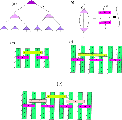
Figure 11: (color online) Graphical representation of TTN. $(a)$ 1D TTN, $(b)$ isometric constraint, 2D TTN for $(c)$ $4\times 4$, $(d)$ $6\times 6$ and $(e)$ $6\times 8$ latices.

We follow Ref. Tagliacozzo et al., 2009 to perform optimization algorithm: the main idea is to take a specific local isomeric tensor—fixing the other tensors—as variational parameters and then obtain variational ground-state energy, so that it becomes minimum. By repeating this process over all other tensors, TTN state would hopefully converge to real ground state. Bond-dimension $\chi$ is our control parameter determining accuracy of algorithm—it is obvious for $\chi\rightarrow\infty$, the result would be exact. Time and memory cost of optimization processing respectively scale by $\mathcal{O}(\chi^{4})$ and $\mathcal{O}(\chi^{3})$. Calculating expectation value of local operators, (nearest neighbor) correlation function and variational energy have also the same cost. In our calculation, we consider clusters up to $8\times 6$ spins, and also do finite-$\chi$ scaling to obtain more accurate result Pollmann et al. (2009). We use the following equation to obtain our final data

$$<\widehat{\mathcal{O}}>_{\chi}=<\widehat{\mathcal{O}}>_{\infty}+\frac{A_{0}}{\chi^{\theta}},$$ (33)

where $<\widehat{\mathcal{O}}>$ stand for expectation value of operators, $A_{0}$ and $\theta$ are two constants—determined by the best fitting methods. Note $<\widehat{\mathcal{O}}>_{\infty}$ is the quantity which is reported throughout the paper. We take $\chi\sim 400$ so that error in variational ground-state energy, in the worst cases (critical point), is of order $10^{-4}$.

References

- Balents Leon (2010) Balents Leon, Nature 464, 199–208 (2010), ISSN 0028-0836.
- Sheckelton J. P. et al. (2012) Sheckelton J. P., Neilson J. R., Soltan D. G., and McQueen T. M., Nat Mater 11, 493–496 (2012), ISSN 1476-1122, URL http://www.nature.com/nmat/journal/v11/n6/abs/nmat3329.html#supplementary-information.
- Doretto and Vojta (2012) R. L. Doretto and M. Vojta, Phys. Rev. B 85, 104416 (2012), URL http://link.aps.org/doi/10.1103/PhysRevB.85.104416.
- Liu et al. (2015) T. Liu, C. Repellin, B. Douçot, N. Regnault, and K. L. Hur, Triplet fflo superconductivity in the doped kitaev-heisenberg honeycomb model (2015), eprint arXiv:1511.03289.
- Harland et al. (2016) M. Harland, M. Katsnelson, and A. Lichtenstein, Plaquette valence bond theory of high-temperature superconductivity (2016), eprint arXiv:1604.01808.
- Nembrini et al. (2016) N. Nembrini, S. Peli, F. Banfi, G. Ferrini, Y. Singh, P. Gegenwart, R. Comin, K. Foyevtsova, A. Damascelli, A. Avella, et al., Tracking local spin-dynamics via high-energy quasi-molecular excitations in a spin-orbit mott insulator (2016), eprint arXiv:1606.01667.
- Xu et al. (2008) C. Xu, M. Müller, and S. Sachdev, Phys. Rev. B 78, 020501 (2008), URL http://link.aps.org/doi/10.1103/PhysRevB.78.020501.
- Singh et al. (1999) R. R. P. Singh, Z. Weihong, C. J. Hamer, and J. Oitmaa, Phys. Rev. B 60, 7278 (1999), URL http://link.aps.org/doi/10.1103/PhysRevB.60.7278.
- Metavitsiadis et al. (2014) A. Metavitsiadis, D. Sellmann, and S. Eggert, Phys. Rev. B 89, 241104 (2014), URL http://link.aps.org/doi/10.1103/PhysRevB.89.241104.
- Isaev et al. (2009) L. Isaev, G. Ortiz, and J. Dukelsky, Phys. Rev. B 79, 024409 (2009), URL http://link.aps.org/doi/10.1103/PhysRevB.79.024409.
- Yu and Kao (2012) J.-F. Yu and Y.-J. Kao, Phys. Rev. B 85, 094407 (2012), URL http://link.aps.org/doi/10.1103/PhysRevB.85.094407.
- Doretto (2014) R. L. Doretto, Phys. Rev. B 89, 104415 (2014), URL http://link.aps.org/doi/10.1103/PhysRevB.89.104415.
- Hu et al. (2013) W.-J. Hu, F. Becca, A. Parola, and S. Sorella, Phys. Rev. B 88, 060402 (2013), URL http://link.aps.org/doi/10.1103/PhysRevB.88.060402.
- Wang et al. (2013) L. Wang, D. Poilblanc, Z.-C. Gu, X.-G. Wen, and F. Verstraete, Phys. Rev. Lett. 111, 037202 (2013), URL http://link.aps.org/doi/10.1103/PhysRevLett.111.037202.
- Gong et al. (2014) S.-S. Gong, W. Zhu, D. N. Sheng, O. I. Motrunich, and M. P. A. Fisher, Phys. Rev. Lett. 113, 027201 (2014), URL http://link.aps.org/doi/10.1103/PhysRevLett.113.027201.
- Morita et al. (2015) S. Morita, R. Kaneko, and M. Imada, Journal of the Physical Society of Japan 84, 024720 (2015), eprint http://dx.doi.org/10.7566/JPSJ.84.024720, URL http://dx.doi.org/10.7566/JPSJ.84.024720.
- Jiang et al. (2012) H.-C. Jiang, H. Yao, and L. Balents, Phys. Rev. B 86, 024424 (2012), URL http://link.aps.org/doi/10.1103/PhysRevB.86.024424.
- Mezzacapo (2012) F. Mezzacapo, Phys. Rev. B 86, 045115 (2012), URL http://link.aps.org/doi/10.1103/PhysRevB.86.045115.
- Li et al. (2012) T. Li, F. Becca, W. Hu, and S. Sorella, Phys. Rev. B 86, 075111 (2012), URL http://link.aps.org/doi/10.1103/PhysRevB.86.075111.
- Ren et al. (2014) Y.-Z. Ren, N.-H. Tong, and X.-C. Xie, Journal of Physics: Condensed Matter 26, 115601 (2014), URL http://stacks.iop.org/0953-8984/26/i=11/a=115601.
- Benyoussef et al. (1998) A. Benyoussef, A. Boubekri, and H. Ez-Zahraouy, Physics Letters A 238, 398 (1998), ISSN 0375-9601, URL http://www.sciencedirect.com/science/article/pii/S0375960197008852.
- Bishop et al. (2008) R. F. Bishop, P. H. Y. Li, R. Darradi, J. Schulenburg, and J. Richter, Phys. Rev. B 78, 054412 (2008), URL http://link.aps.org/doi/10.1103/PhysRevB.78.054412.
- Yamaki et al. (2013) S. Yamaki, K. Seki, and Y. Ohta, Phys. Rev. B 87, 125112 (2013), URL http://link.aps.org/doi/10.1103/PhysRevB.87.125112.
- Higashinaka et al. (2015) R. Higashinaka, T. Asano, T. Nakashima, K. Fushiya, Y. Mizuguchi, O. Miura, T. D. Matsuda, and Y. Aoki, Journal of the Physical Society of Japan 84, 023702 (2015), eprint http://dx.doi.org/10.7566/JPSJ.84.023702, URL http://dx.doi.org/10.7566/JPSJ.84.023702.
- Nisoli et al. (2013) C. Nisoli, R. Moessner, and P. Schiffer, Rev. Mod. Phys. 85, 1473 (2013), URL http://link.aps.org/doi/10.1103/RevModPhys.85.1473.
- Suzuki et al. (2012) S. Suzuki, J. ichi Inoue, and B. K. Chakrabarti, Quantum Ising Phases and Transitions in Transverse Ising Models (Lecture Notes in Physics) (Springer, 2012), ISBN 364233038X, URL http://link.springer.com/book/10.1007%2F978-3-642-33039-1.
- Kalz et al. (2009) A. Kalz, A. Honecker, S. Fuchs, and T. Pruschke, Journal of Physics: Conference Series 145, 012051 (2009), URL http://stacks.iop.org/1742-6596/145/i=1/a=012051.
- Amit Dutta (2010) B. K. C. U. D. T. F. R. D. S. Amit Dutta, Gabriel Aeppli, Quantum phase transitions in transverse field spin models: from statistical physics to quantum information (2010), eprint arXiv:1012.0653.
- Henry et al. (2012) L.-P. Henry, P. C. W. Holdsworth, F. Mila, and T. Roscilde, Phys. Rev. B 85, 134427 (2012), URL http://link.aps.org/doi/10.1103/PhysRevB.85.134427.
- Ganesh et al. (2013) R. Ganesh, S. Nishimoto, and J. van den Brink, Phys. Rev. B 87, 054413 (2013), URL http://link.aps.org/doi/10.1103/PhysRevB.87.054413.
- Sadrzadeh, Marzieh and Langari, Abdollah (2015) Sadrzadeh, Marzieh and Langari, Abdollah, Eur. Phys. J. B 88, 259 (2015), URL http://dx.doi.org/10.1140/epjb/e2015-60142-2.
- Verstraete et al. (2008) F. Verstraete, V. Murg, and J. Cirac, Adv. Phys. 57, 143 (2008), URL http://dx.doi.org/10.1080/14789940801912366.
- Leggett (1980) A. J. Leggett, Progress of Theoretical Physics Supplement 69, 80 (1980), URL http://ptps.oxfordjournals.org/content/69/80.abstract.
- Abad and Karimipour (2016) T. Abad and V. Karimipour, Phys. Rev. B 93, 195127 (2016), URL http://link.aps.org/doi/10.1103/PhysRevB.93.195127.
- Oitmaa (1981) J. Oitmaa, Journal of Physics A: Mathematical and General 14, 1159 (1981), URL http://stacks.iop.org/0305-4470/14/i=5/a=035.
- Morán-López et al. (1993) J. L. Morán-López, F. Aguilera-Granja, and J. M. Sanchez, Phys. Rev. B 48, 3519 (1993), URL http://link.aps.org/doi/10.1103/PhysRevB.48.3519.
- Nishimori and Ortiz (2011) H. Nishimori and G. Ortiz, Elements of Phase Transitions and Critical Phenomena (Oxford University Press, 2011), ISBN 9780199577224, URL https://global.oup.com/academic/product/elements-of-phase-transitions-and-critical-phenomena-9780199577224?cc=us&lang=en&.
- Chubukov and Jolicoeur (1991) A. V. Chubukov and T. Jolicoeur, Phys. Rev. B 44, 12050 (1991), URL http://link.aps.org/doi/10.1103/PhysRevB.44.12050.
- Zhitomirsky and Ueda (1996) M. E. Zhitomirsky and K. Ueda, Phys. Rev. B 54, 9007 (1996), URL http://link.aps.org/doi/10.1103/PhysRevB.54.9007.
- Cai et al. (2007) Z. Cai, S. Chen, S. Kou, and Y. Wang, Phys. Rev. B 76, 054443 (2007), URL http://link.aps.org/doi/10.1103/PhysRevB.76.054443.
- Jiang et al. (2009) H. C. Jiang, F. Krüger, J. E. Moore, D. N. Sheng, J. Zaanen, and Z. Y. Weng, Phys. Rev. B 79, 174409 (2009), URL http://link.aps.org/doi/10.1103/PhysRevB.79.174409.
- Colpa (1978) J. Colpa, Physica A: Statistical Mechanics and its Applications 93, 327 (1978), ISSN 0378-4371, URL http://www.sciencedirect.com/science/article/pii/0378437178901607.
- Sachdev and Bhatt (1990) S. Sachdev and R. N. Bhatt, Phys. Rev. B 41, 9323 (1990), URL http://link.aps.org/doi/10.1103/PhysRevB.41.9323.
- Eisert et al. (2010) J. Eisert, M. Cramer, and M. B. Plenio, Rev. Mod. Phys. 82, 277 (2010), URL http://link.aps.org/doi/10.1103/RevModPhys.82.277.
- Efrati et al. (2014) E. Efrati, Z. Wang, A. Kolan, and L. P. Kadanoff, Rev. Mod. Phys. 86, 647 (2014), URL http://link.aps.org/doi/10.1103/RevModPhys.86.647.
- Gerster et al. (2014) M. Gerster, P. Silvi, M. Rizzi, R. Fazio, T. Calarco, and S. Montangero, Phys. Rev. B 90, 125154 (2014), URL http://link.aps.org/doi/10.1103/PhysRevB.90.125154.
- Evenbly and Vidal (2009) G. Evenbly and G. Vidal, Phys. Rev. B 79, 144108 (2009), URL http://link.aps.org/doi/10.1103/PhysRevB.79.144108.
- Tagliacozzo et al. (2009) L. Tagliacozzo, G. Evenbly, and G. Vidal, Phys. Rev. B 80, 235127 (2009), URL http://link.aps.org/doi/10.1103/PhysRevB.80.235127.
- Pollmann et al. (2009) F. Pollmann, S. Mukerjee, A. M. Turner, and J. E. Moore, Phys. Rev. Lett. 102, 255701 (2009), URL http://link.aps.org/doi/10.1103/PhysRevLett.102.255701.