Multi-flavor string-net models

Abstract

We generalize the string-net construction to multiple flavors of strings, each of which is labeled by the elements of an abelian group $G_{i}$. The same flavor of strings can branch while different flavors of strings can cross one another and thus they form intersecting string-nets. We systematically construct the exactly soluble lattice Hamiltonians and the ground state wave functions for the intersecting string-net condensed phases. We analyze the braiding statistics of the low energy quasiparticle excitations and find that our model can realize all the topological phases as the string-net model with group $G=\prod_{i}G_{i}$. In this respect, our construction suggests several ways of building lattice models which realize topological order $G$. They correspond to intersecting string-net models with various choices of flavors of strings associated with different decomposition of $G$. In fact, our construction concretely demonstrates the Künneth formula by constructing various lattice models with the same topological order. As an example, we construct the $G=\mathbb{Z}_{2}\times\mathbb{Z}_{2}\times\mathbb{Z}_{2}$ string-net model which realizes a non-abelian topological phase by properly intersecting three copies of toric codes.

I Introduction

Topological phases are gapped quantum phases of matter which support quasiparticle excitations with fractional statistics Wen (2007). The classical examples of topological phases include fractional quantum Hall states and spin liquids. These phases can not be understood by the Landau symmetry breaking theory. Thus it requires new approaches to study them. One useful approach is the construction of exactly soluble lattice models that realize these topological phases.

The toric code model of Ref. Kitaev, 2003 is one of the simplest examples of exactly soluble lattice model which realizes $\mathbb{Z}_{2}$ topological order. The model is a spin-1/2 system with spins living on the links of the square lattice. The Hamiltonian is a sum of commuting projectors and thus is exactly soluble. One interesting aspect of toric code model is that its ground state can be thought of as a closed loop condensate. Levin and WenLevin and Wen (2005) generalized this picture and constructed the “string-net” models whose low energy effective degrees of freedom are extended objects called string-nets—a network of strings.

Like the toric code, the string-net modelsLevin and Wen (2005) are also exactly soluble lattice spin models which can realize a large class of topological phases such as phases whose low energy effective theories are finite lattice gauge theories and doubled Chern-Simons theories. Recently, the string-net construction was generalizedLevin and Wen (2005); Lan and Wen (2014); Hu et al. (2013); Mesaros and Ran (2013); Kitaev and Kong (2012); Kong (2014) to realize all topological phases which support a gapped edge.

The string-net models provide a nice physical picture for realizing topological phases–condensation of string-nets. In this paper, we extend the picture to multiple flavors of string-nets. One way to think of different flavors of string-nets is to imagine a multi-layer system where various string-nets sit on different layers. We can then obtain a two-dimensional system with multi-flavor string-nets by letting the layer spacing $d\rightarrow 0$. In this way, string-nets of the same flavor can branch and string-nets of different flavors cross one another. Thus they form intersecting string-nets. We ask the question: what topological phases can be obtained from the intersecting string-nets?

We answer this question for a simpler case where each flavor of string-nets is associated with an abelian group $G_{i}$. Depending on the interactions between different flavors of string-nets, we may obtain various topological phases. In the work, we restrict our attention to the subset of interactions which do not change the string types, namely the interactions are diagonal in the string-net state basis.

Our analysis is based on an explicit construction: we systematically construct all intersecting string-net models with interactions between different flavors of string-nets. For each model, we analyze the quasiparticle braiding statistics. From this analysis, we find that the multi-flavor string-net model can realize all the topological phases as the string-net model with $G=\prod_{i}G_{i}$. In this regard, multi-flavor string-net models associated with $\{G_{i}\}$ can be viewed as an alternative construction of the original string-net models with $G$. Moreover, our construction also provides several ways to build lattice models with topological order $G$ corresponding to various decomposition of $G$ into $G=\prod_{i}G_{i}$ and thus different flavors of string-nets.

Specifically, our construction starts with a set of string-net models with $\{G_{i}\}$ associated with each flavor of string-nets. We then intersect/stack the set of string-net models in a proper way so that the resulting model is exactly soluble. We find that the model realizes all topological phases with topological order $G=\prod_{i}G_{i}$. One can also start with the other set of string-net models with $\{G_{i}^{\prime}\}$ such that $G=\prod_{i}G_{i}^{\prime}$. Our construction then gives a different exactly soluble model which also realizes topological order $G$.

Intuitively, one can imagine that we decompose the string labeled by the elements of $G$ into multiple strings each of which is labeled by the elements of $G_{i}$ such that $G=\prod_{i}G_{i}$. We then put each component string into an individual string-net model. However, these component strings are not independent but satisfy certain constraints. These constraints dictate how different component strings intersect with one another. As a result, the model built from the intersecting string-net models with $\{G_{i}\}$ associated with the component strings gives a “parton” construction of the string-net model with $G=\prod_{i}G_{i}$. Like the usual parton construction of particles, we have various ways of decomposing strings while they all describe the same topological phases.

In contrast to the original string-net models whose input is a set of complex functions $F$ which satisfy 3-cocycle conditions, we encode the information of $F$ into simpler objects, called $F^{(2)},F^{(3)}$, which satisfy 2-cocycle and 1-cocycle conditions respectively. The objects $F^{(2)}$ and $F^{(3)}$ are associated with intersections between two and three flavors of string-nets. It turns out that the underlying mathematical structure of our construction is the Künneth formula.

The advantage of using $F^{(2)}$ and $F^{(3)}$ objects as input is that it provides a simple way to construct models which realize a “twisted” topological phase. For example, one can start with 3 copies of toric codes and then intersect them with properly chosen $F^{(3)}$. The resulting model can realize a twisted $\mathbb{Z}_{2}\times\mathbb{Z}_{2}\times\mathbb{Z}_{2}$ gauge theory. Interestingly, this model supports non-abelian quasiparticle excitations which will be discussed in detail later.

The paper is organized as follows. In Sec. II, we review some basics of string-net models and abelian string-net models. In Sec. III, we warm up by constructing ground state wave functions with one flavor of abelian string-nets. In Sec. IV, V, we generalize to construct ground state wave functions and lattice Hamiltonians for multi-flavor string-net models. We analyze the low energy quasiparticle excitations of these models in Sec. VI. In Sec. VII, we explicitly compute the quasiparticle braiding statistics for general abelian string-net models. We discuss the relation between different constructions associated with different choices of flavors of string-nets in Sec. IX. Finally we illustrate our new construction with concrete examples in Sec. X. The mathematical details can be found in appendices.

II Review of string-net models

In this section, we briefly review the basic structure of string-nets and string-net models. We mainly focus on a special class of string-net models–abelian string-net models. The materials in this section are adapted from Ref. Lin and Levin, 2014.

A string-net is a network of strings. The strings can come in different types and carry orientations. In this paper, we focus on trivalent networks in two-dimensional space, namely, exactly 3 strings meet at each branch point or node in the network. Thus, we can think of string-nets as trivalent graphs with labeled and oriented edges in the plane (in the continuum or on a lattice).

A string-net model is a quantum mechanical model which describe the dynamics of the string-nets. To specify a string-net model, one has to provide several pieces of data. First, one has to specify a finite set of string types $\left\{a,b,c,...\right\}.$ Second, one has to specify the dual string type $a^{\ast}$ of each string type $a.$ A string $a$ with a given orientation corresponds to the same physical state as a string $a^{\ast}$ with the opposite orientation. Finally, one has to specify the branching rules. The branching rules are the set of all triplets of string types $\left\{\left(a,b,c\right),...\right\}$ which are allowed to meet at a point.

It is also convenient to include the null string type into the formalism. The null string type, denoted by $0,$ is equivalent to no string at all. This string type is self-dual: $0^{\ast}=0$ and thus we will neglect the orientation of the null string. The associated branching rule is that $\left(0,a,b\right)$ is allowed if $a=b^{\ast}.$

The abelian string-net models are a special class of string-net models associated with abelian groups. To construct an abelian string-net model associated with a finite abelian group $G,$ we first label the string types by the elements of the group $a\in G$ with null string being the identity element $0.$ Second, we define the dual string $a^{\ast}$ as the group inverse: $a^{\ast}=-a.$ Finally, we define branching rules by

$$\left(a,b,c\right)\text{ is allowed if }a+b+c=0.$$

(Here we use additive notation for the group operation.)

So far we focused on the Hilbert space of the string-net model. We also need to specify the Hamiltonian. A typical string-net Hamiltonian is a sum of a kinetic energy term and a string tension term. The kinetic energy term gives an amplitude for the string-net states to move while the string tension term gives an energy cost to large string-nets. Depending on the relative size of the two terms, we have two quantum phases. When the string tension term dominates, the ground state will contain only a few small strings. When the kinetic energy term dominates, the ground state will be a superposition of many large string-net configuration–a string-net condensed phase.

The string-net condensed phases are known to support excitations with fractional statistics. The wave functions and the corresponding exactly soluble Hamiltonians for these topological phases are constructed systematically in Ref. Levin and Wen, 2005. In this paper, we will generalize their construction to the Hilbert space which consists of multiple flavors of string-nets, each of which is associated with a group $G_{i}$.

III Single-flavor string-net wave functions

In this section, we review the wave functions and Hamiltonian for abelian string-net condensed phases. The materials are adapted from Ref. Lin and Levin, 2014.

We start with the ground state wave functions for string-net condensed phases. The wave functions are defined implicitly using local constraint equations. More specifically, the local constraint equations take the following graphical form:

$$\Phi\left(\raisebox{-11.56346pt}{\includegraphics[height=28.90755pt]{rule0a1.eps}}\right) = \Phi\left(\raisebox{-11.56346pt}{\includegraphics[height=28.90755pt]{rule0b1.eps}}\right),$$ (1)

$$\Phi\left(\raisebox{-11.56346pt}{\includegraphics[height=28.90755pt]{rule1a1.eps}}\right) = d_{a}\Phi\left(\raisebox{-11.56346pt}{\includegraphics[height=28.90755pt]{rule1b1.eps}}\right),$$ (2)

$$\Phi\left(\raisebox{-11.56346pt}{\includegraphics[height=28.90755pt]{rule2a1.eps}}\right) = F(a,b,c)\Phi\left(\raisebox{-11.56346pt}{\includegraphics[height=28.90755pt]{rule2b1.eps}}\right).$$ (3)

Here $a,b,c\,$are arbitrary string types and the shaded regions represent arbitrary string-net configurations which is unchanged. The $d_{a}$ and $F\left(a,b,c\right)$ are complex numbers which satisfy certain algebraic equations we will specify below.

The idea of Eqs. (1–3) is that we can relate the amplitude of any string-net configuration to the amplitude of the vacuum (no-string) configuration by applying the local rules multiple times. We use the convention that

$$\Phi\left(\text{vacuum}\right)=1,$$

and then the amplitude of any configuration is fully determined. Thus, the string-net wave function is fully determined once the parameters $d_{a},\gamma_{a},\alpha(a,b),F(a,b,c)$ are given.

To construct the most general abelian string-net models, we need two additional ingredients $\gamma,\alpha$. First, the $\gamma$ is a $\mathbb{Z}_{2}$ phase factor associated with vertices with one null string and two opposite oriented strings:

$$\left\langle\raisebox{-11.56346pt}{\includegraphics[height=28.90755pt]{rule4a1.eps}}\right| =\gamma_{a}\left\langle\raisebox{-11.56346pt}{\includegraphics[height=28.90755pt]{rule4b1.eps}}\right|,$$ (4)

$$\left\langle\raisebox{-11.56346pt}{\includegraphics[height=28.90755pt]{rule5a1.eps}}\right| =\gamma_{a}\left\langle\raisebox{-11.56346pt}{\includegraphics[height=28.90755pt]{rule5b1.eps}}\right|.$$

Here $\gamma_{a}$ can be chosen to be $\pm 1$ without loss of generality. A pair of null strings with opposite orientations can be erased in pairs according to:

$$\left\langle\raisebox{-11.56346pt}{\includegraphics[height=28.90755pt]{rule6b1.eps}}\right|=\left\langle\raisebox{-11.56346pt}{\includegraphics[height=28.90755pt]{rule6c1.eps}}\right|=\left\langle\raisebox{-11.56346pt}{\includegraphics[height=28.90755pt]{rule6a1.eps}}\right|.$$ (5)

Second, to define $\alpha,$ we absorbed the end of the null strings into vertices by defining:

$$\left\langle\raisebox{-11.56346pt}{\includegraphics[height=28.90755pt]{vertex2a.eps}}\right| =\left\langle\raisebox{-11.56346pt}{\includegraphics[height=28.90755pt]{vertex2.eps}}\right|,$$

$$\left\langle\raisebox{-11.56346pt}{\includegraphics[height=28.90755pt]{vertex3a.eps}}\right| =\left\langle\raisebox{-11.56346pt}{\includegraphics[height=28.90755pt]{vertex3.eps}}\right|,$$

$$\left\langle\raisebox{-11.56346pt}{\includegraphics[height=28.90755pt]{vertex4a.eps}}\right| =\left\langle\raisebox{-11.56346pt}{\includegraphics[height=28.90755pt]{vertex4.eps}}\right|.$$

Here we decorate the vertices that have three incoming or three outgoing legs with dots. The dots can be placed in any of the three positions near the vertex. Then, the $\mathbb{Z}_{3}$ phase factor $\alpha$ is defined by

$$\left\langle\raisebox{-11.56346pt}{\includegraphics[height=28.90755pt]{rule3a1.eps}}\right| =\alpha\left(a,b\right)\left\langle\raisebox{-11.56346pt}{\includegraphics[height=28.90755pt]{rule3b1.eps}}\right|$$

$$\left\langle\raisebox{-11.56346pt}{\includegraphics[height=28.90755pt]{rule3c1.eps}}\right| =\alpha\left(a,b\right)\left\langle\raisebox{-11.56346pt}{\includegraphics[height=28.90755pt]{rule3d1.eps}}\right|.$$

The $\alpha\left(a,b\right)$ can be chosen to be a third root of unity without loss of generality. They are designed to keep track of the orientation of vertices. Note that flipping the null string or moving the position of the dot does not change the physical state, but it can introduce a phase factor $\gamma_{a}$ or $\alpha\left(a,b\right).$ These phases $\gamma_{a},\alpha\left(a,b\right)$ are closely related to so-called $\mathbb{Z}_{2}$ and $\mathbb{Z}_{3}$ Frobenius-Schur indicatorsKitaev (2006)Bonderson (2007).

So far the parameters $\left\{d_{a},F\left(a,b,c\right),\gamma,\alpha\right\}$ are arbitrary. However, these parameters have to satisfy a set of algebraic equations so that they lead to self-consistent local rules and a well-defined wave function $\Phi:$

$$F\left(a+b,c,d\right) F\left(a,b,c+d\right)=$$ (6a)

$$F\left(a,b,c\right)F\left(a,b+c,d\right)F\left(b,c,d\right),$$

$$F\left(a,b,c\right) =1\text{ if }a\text{ or }b\text{ or }c=0,$$ (6b)

$$d_{a}d_{b} =d_{a+b},$$ (6c)

$$\gamma_{a} =F\left(a^{\ast},a,a^{\ast}\right)d_{a},$$ (6d)

$$\alpha\left(a,b\right) =F\left(a,b,\left(a+b\right)^{\ast}\right)\gamma_{a+b}.$$ (6e)

In addition, to construct a consistent string-net model (Hamiltonian), we need one more constraint

$$\left|F\left(a,b,c\right)\right|=1.$$

This constraint ensures the corresponding exactly soluble Hamiltonians to be Hermitian.

For each solution to the above constraints, we can construct a well-defined wave function and an exactly soluble Hamiltonian. However, if two sets of solutions $\left\{F,d,\alpha,\gamma\right\},\left\{\tilde{F},\tilde{d},\tilde{\alpha},\tilde{\gamma}\right\}$ are related by gauge transformations (see Ref. Lin and Levin, 2014 for details), the two solutions are equivalent and the corresponding wave functions $\Phi,\tilde{\Phi}$ and Hamiltonians can be transformed into one another by a local unitary transformation. Thus it implies that $\Phi,\tilde{\Phi}$ describe the same quantum phase. Therefore, one only need to consider one solution within each gauge equivalence class to construct distinct topological phases.

IV Multi-flavor string-net wave functions

In this section, we study the wave functions for multiple flavors of string-nets. For each flavor-$i$ of strings, we label the string types by the elements of the group $G_{i}:\{a_{i},b_{i},c_{i},\dots\}$. The strings of the same flavor-$i$ can branch according to the branching rules $\{(a_{i},b_{i},c_{i}),\dots\}$ and form the string-nets of flavor-$i$. On the other hand, different flavors of strings can intersect/cross one another and thus form the intersecting string-nets of multiple flavors. To describe the wave functions for the intersecting string-nets, we need additional rules to describe how different flavors of string-nets intersect with one another. In two dimensions, it is sufficient to consider two kinds of intersections: intersections between two flavors of string-nets and intersections among three flavors of string-nets. In this section, we introduce new local rules for the multi-flavor string-net wave functions. In section V, we will show that these wave functions are the ground states of the exactly soluble multi-flavor string-net Hamiltonians, defined on a lattice.

IV.1 Local rules ansatz

Let us consider $L$ flavors of string-nets. We label the string types of the $i$-th flavor by $\left\{a_{i},b_{i},...\right\}$ with the flavor index $i=1,...,L$. Like single-flavor string-nets, each flavor of string-nets satisfy the original local rules (1–3) individually. In addition, since different flavors of string-nets can intersect, we require new local rules to describe the wave functions $\Phi$ for the intersecting string-nets. In particular, we consider intersections between two flavors of string-nets with flavor indices $i\neq$ $j$ and intersections among three flavors of string-nets with $i\neq j\neq k$. Once we specify these two kinds of intersections, the whole string-net configuration is uniquely determined.

Specifically, these new local rules for constructing intersecting string-net wave function $\Phi$ can be put in the following graphical forms

$$\Phi\left(\raisebox{-11.56346pt}{\includegraphics[height=28.90755pt]{rule1a.eps}}\right) =F_{a_{i}}^{\left(2\right)}\left(a_{j},b_{j}\right)\Phi\left(\raisebox{-11.56346pt}{\includegraphics[height=28.90755pt]{rule1b.eps}}\right),$$ (7)

$$\Phi\left(\raisebox{-11.56346pt}{\includegraphics[height=28.90755pt]{rule10a.eps}}\right) =\bar{F}_{a_{i}}^{\left(2\right)}\left(a_{j},b_{j}\right)\Phi\left(\raisebox{-11.56346pt}{\includegraphics[height=28.90755pt]{rule10b.eps}}\right)\text{ },$$ (8)

$$\Phi\left(\raisebox{-7.22743pt}{\includegraphics[height=21.68121pt]{rule2a.eps}}\right) =\kappa_{a_{i}}\left(a_{j}\right)\Phi\left(\raisebox{-7.22743pt}{\includegraphics[height=21.68121pt]{rule2b.eps}}\right),$$ (9)

$$\Phi\left(\raisebox{-7.22743pt}{\includegraphics[height=19.5132pt]{rule3a.eps}}\right) =\eta_{a_{i}}\left(a_{j}\right)\Phi\left(\raisebox{-7.22743pt}{\includegraphics[height=19.5132pt]{rule3b.eps}}\right),$$ (10)

$$\Phi\left(\raisebox{-11.56346pt}{\includegraphics[height=28.90755pt]{rule4a.eps}}\right) =F_{a_{i}}^{\left(3\right)}\left(a_{j},a_{k}\right)\Phi\left(\raisebox{-11.56346pt}{\includegraphics[height=28.90755pt]{rule4b.eps}}\right).$$ (11)

Here the subindices $i,j,k$ indicate the three different flavors of string-nets. Note that we only draw the part of configuration which is changed and neglect other part which is unchanged. Namely, the graphs in these rules are understood as being with fixed end points which connect to other unchanged part of the string-net configuration. The $F_{a_{i}}^{\left(2\right)}\left(a_{j},b_{j}\right),$ $\bar{F}_{a_{i}}^{\left(2\right)}\left(a_{j},b_{j}\right),\kappa_{a_{i}}\left(a_{j}\right)$ and $\eta_{a_{i}}\left(a_{j}\right)$ are complex numbers that depend on two flavors of string-nets while the $F_{a_{i}}^{\left(3\right)}\left(a_{j},a_{k}\right)$ are complex numbers that depend on three flavors of string-nets.

The first four rules (7–10)involve two flavors of string-nets while the last rule (11) involves three flavors of string-nets. For these five rules, it is understood that the value of $\Phi$ depends only on the topology of the intersecting string-net configurations. That is, two configurations have the same value of $\Phi$ if one can be smoothly deformed into one another without changing the number of crossings between each two of strings This symmetry will put some constraints on the parameters $F^{\left(2\right)},\bar{F}^{\left(2\right)},\kappa,\eta,F^{\left(3\right)}$ which we will discuss in the next section.

We now discuss the meanings of these new local rules. The first rule (7) says that one can glide a string $a_{i}$ across the vertex of the string-nets of different flavor $\left\{a_{j},b_{j},a_{j}+b_{j}\right\}$ with the amplitude of the final configuration related to the amplitude of the original configuration by a phase $F_{a_{i}}^{\left(2\right)}\left(a_{j},b_{j}\right).$ The second rule (8) is similar to the first rule (7) but with the orientation of $a_{i}$ reversed. Similarly, the third rule (9) dictates that one can glide a string $a_{i}$ across the vertex of the string-nets of different flavor with one null string $\left\{b_{j},b_{j}^{\ast},0\right\}$ with the relative amplitude of two configurations being $\kappa_{a_{i}}\left(a_{j}\right)$. The fourth rule (10) says that the amplitudes of two configurations which are related by deforming one string $a_{i}$ across the other string $a_{j}$ of different flavor differ by a phase $\eta_{a_{i}}\left(a_{j}\right)$. The last rule (11) depicts that one can glide a string $a_{i}$ across the intersection of the other two strings $a_{j},a_{k}$ where three strings are of different flavors. The amplitude of resulting configuration is related to the amplitude of the original configuration by a phase $F_{a_{i}}^{\left(3\right)}\left(a_{j},a_{k}\right).$

By applying these new local rules (7–11) multiple times, one can disentangle all different flavors of string-nets. Then we apply the original local rules (1–3) for each flavor of string-nets and relate the amplitude of any string-net configuration to the amplitude of vacuum. Accordingly, the rules determine the wave functions of intersecting string-nets once the parameters $\left\{d,F,\gamma,\alpha,F^{\left(2\right)},\bar{F}^{\left(2\right)},\eta,\kappa,F^{\left(3\right)}\right\}$ are given.

Before we discuss the constraints which these parameters have to satisfy, we discuss some corollaries of (7–10). First, the rules (5) and (9) imply that

$$\Phi\left(\raisebox{-7.22743pt}{\includegraphics[height=21.68121pt]{rule2c.eps}}\right)=\kappa_{a_{i}}\left(a_{j}\right)^{-1}\Phi\left(\raisebox{-7.22743pt}{\includegraphics[height=21.68121pt]{rule2d.eps}}\right).$$ (12)

We can also flip the null string of (9,12) by applying (4) to both sides of the two equations.

Second, the rules (2) and (10) imply that

$$\Phi\left(\raisebox{-7.22743pt}{\includegraphics[height=19.5132pt]{rule3ai.eps}}\right)=\eta_{a_{i}}\left(a_{j}\right)\Phi\left(\raisebox{-7.22743pt}{\includegraphics[height=19.5132pt]{rule3bi.eps}}\right).$$ (13)

Together with the rules (7,8,10), one can derive the following relations

$$\Phi\left(\raisebox{-11.56346pt}{\includegraphics[height=28.90755pt]{rule11a.eps}}\right)=\frac{F_{a_{i}}^{\left(2\right)}\left(a_{j},b_{j}\right)\eta_{a_{i}}\left(b_{j}\right)}{\eta_{a_{i}}\left(a_{j}+b_{j}\right)}\Phi\left(\raisebox{-11.56346pt}{\includegraphics[height=28.90755pt]{rule11b.eps}}\right),$$ (14)

$$\Phi\left(\raisebox{-11.56346pt}{\includegraphics[height=28.90755pt]{rule12a.eps}}\right)=\frac{\bar{F}_{a_{i}}^{\left(2\right)}\left(a_{j},b_{j}\right)\eta_{a_{i}}\left(b_{j}\right)}{\eta_{a_{i}}\left(a_{j}+b_{j}\right)}\Phi\left(\raisebox{-11.56346pt}{\includegraphics[height=28.90755pt]{rule12b.eps}}\right),$$ (15)

$$\Phi\left(\raisebox{-11.56346pt}{\includegraphics[height=28.90755pt]{rule13a.eps}}\right)=\frac{\bar{F}_{a_{i}}^{\left(2\right)}\left(a_{j},b_{j}\right)\eta_{a_{i}}\left(a_{j}\right)}{\eta_{a_{i}}\left(a_{j}+b_{j}\right)}\Phi\left(\raisebox{-11.56346pt}{\includegraphics[height=28.90755pt]{rule13b.eps}}\right),$$ (16)

$$\Phi\left(\raisebox{-11.56346pt}{\includegraphics[height=28.90755pt]{rule14a.eps}}\right)=\frac{F_{a_{i}}^{\left(2\right)}\left(a_{j},b_{j}\right)\eta_{a_{i}}\left(a_{j}\right)}{\eta_{a_{i}}\left(a_{j}+b_{j}\right)}\Phi\left(\raisebox{-11.56346pt}{\includegraphics[height=28.90755pt]{rule14b.eps}}\right).$$ (17)

These relations allow us to glide a string $a_{i}$ with various orientations across the vertex of the string-nets of different flavor $\left\{a_{j},b_{j},a_{j}+b_{j}\right\}$.

The first equation (14) can be shown by considering

$$\Phi\left(\raisebox{-11.56346pt}{\includegraphics[height=28.90755pt]{rule11a.eps}}\right)=\eta_{a_{i}}\left(b_{j}\right)\Phi\left(\raisebox{-11.56346pt}{\includegraphics[height=28.90755pt]{rule11c.eps}}\right)$$

$$=\eta_{a_{i}}\left(b_{j}\right)F_{a_{i}}\left(a_{j},b_{j}\right)\Phi\left(\raisebox{-11.56346pt}{\includegraphics[height=28.90755pt]{rule11d.eps}}\right)$$

$$=F_{a_{i}}^{\left(2\right)}\left(a_{j},b_{j}\right)\frac{\eta_{a_{i}}\left(b_{j}\right)}{\eta_{a_{i}}\left(a_{j}+b_{j}\right)}\Phi\left(\raisebox{-11.56346pt}{\includegraphics[height=28.90755pt]{rule11b.eps}}\right).$$

This shows (14). Similarly, (15-17) can be shown by the same manner.

Finally, from the rules (9,11) and (5), one can obtain

$$\Phi\left(\raisebox{-11.56346pt}{\includegraphics[height=28.90755pt]{rule14c.eps}}\right)=F^{(3)}_{a_{i}^{*}}(a_{j},a_{k})\Phi\left(\raisebox{-11.56346pt}{\includegraphics[height=28.90755pt]{rule14d.eps}}\right).$$ (18)

IV.2 Self-consistency conditions

To have a well-defined intersecting string-net wave function $\Phi,$ the parameters $\left\{d,F,\gamma,\alpha\right\}$ need to satisfy (6) for each flavor of string-nets and the parameters $\left\{F^{\left(2\right)},\bar{F}^{\left(2\right)},\kappa,\eta,F^{\left(3\right)}\right\}$ have to satisfy the following constraints:

$$F_{a_{i}}^{\left(2\right)}\left(a_{j},b_{j}\right)F_{a_{i}}^{\left(2\right)}\left(a_{j}+b_{j},c_{j}\right)$$ (19a)

$$\quad\ \ \ \ \ \ \ \ \ =F_{a_{i}}^{\left(2\right)}\left(b_{j},c_{j}\right)F_{a_{i}}^{\left(2\right)}\left(a_{j},b_{j}+c_{j}\right),$$

$$\bar{F}_{a_{i}}^{\left(2\right)}\left(a_{j},b_{j}\right)=F_{a_{i}^{\ast}}^{\left(2\right)}\left(a_{j},b_{j}\right)\frac{\kappa_{a_{j}}\left(a_{i}^{\ast}\right)\kappa_{b_{j}}\left(a_{i}^{\ast}\right)}{\kappa_{a_{j}+b_{j}}\left(a_{i}^{\ast}\right)},$$ (19b)

$$\frac{F_{a_{i}}^{\left(2\right)}\left(a_{j},b_{j}\right)F_{b_{i}}^{\left(2\right)}\left(a_{j},b_{j}\right)}{F_{a_{i}+b_{i}}^{\left(2\right)}\left(a_{j},b_{j}\right)}=\frac{\bar{F}_{a_{j}}^{\left(2\right)}\left(a_{i},b_{i}\right)\bar{F}_{b_{j}}^{\left(2\right)}\left(a_{i},b_{i}\right)}{\bar{F}_{a_{j}+b_{j}}^{\left(2\right)}\left(a_{i},b_{i}\right)},$$ (19c)

$$\kappa_{a_{i}}\left(a_{j}\right)\kappa_{a_{i}^{\ast}}\left(a_{j}^{\ast}\right)\kappa_{a_{j}^{\ast}}\left(a_{i}\right)\kappa_{a_{j}}\left(a_{i}^{\ast}\right)=1,$$ (19d)

$$\kappa_{a_{i}}\left(a_{j}\right)=\eta_{a_{i}}\left(a_{j}\right)F_{a_{i}}^{\left(2\right)}\left(a_{j}^{\ast},a_{j}\right),$$ (19e)

$$F_{a_{i}}^{\left(3\right)}\left(a_{j},a_{k}\right)F_{a_{i}}^{\left(3\right)}\left(b_{k}^{\ast},a_{j}\right)=F_{a_{i}}^{\left(3\right)}\left(a_{j},a_{k}+b_{k}\right),$$ (19f)

$$F^{(3)}_{a_{i}}(a_{j},a_{k})F^{(3)}_{b_{i}}(a_{j},a_{k})=F^{(3)}_{a_{i}+b_{i}}(a_{j},a_{k}),$$ (19g)

$$\eta_{a_{i}}\left(a_{j}\right)=\eta_{a_{j}}\left(a_{i}\right),$$ (19h)

$$F_{a_{i}}^{\left(3\right)}\left(a_{j},a_{k}\right)=F_{a_{j}^{\ast}}^{\left(3\right)}\left(a_{k},a_{i}\right)^{-1}=F_{a_{i}^{\ast}}^{\left(3\right)}\left(a_{j}^{\ast},a_{k}^{\ast}\right)^{-1},$$ (19i)

$$F_{a_{i}}^{\left(2\right)}\left(a_{j},b_{j}\right)=F_{a_{i}}^{\left(3\right)}\left(a_{j},a_{k}\right)=1\text{ if }a\text{ or }b=0.$$ (19j)

The first equation (19a) can be understood by considering the sequence of manipulations shown in Fig. 1. The amplitude of (c) can be obtained from (a) in two different ways. For the rule to be consistent, $F^{\left(2\right)}$ must satisfy (19a). The other conditions (19b–19g) can be derived from similar consistency requirement (see appendix A). Eq. (19h) comes from the symmetry of the roles of two strings of different flavors $a_{i},a_{j}$ in the rule (10). Similarly, Eq. (19i) follows from the symmetry of the roles of three strings of different flavors $a_{i},a_{j},a_{k}$ in the rule (11). The last condition (19j) simply says that gliding a null string around the other string gives no phase factor to the amplitude of the final string-net configuration.

We see from (19b), it is sufficient to solve $\left\{F^{\left(2\right)},\kappa,\eta,F^{\left(3\right)}\right\}.$ Once we have solutions to $\left\{F^{\left(2\right)},\kappa,\eta,F^{\left(3\right)}\right\},$ the $\bar{F}^{\left(2\right)}$ can determined by $\left(\ref{fbar}\right).$ Specifically, Eqs. (19a–19d) determine $F^{(2)},\kappa$. With $F^{(2)},\kappa$, Eqs. (19e,19h) then determine $\eta$. Finally, Eqs. (19f,19g,19i) determine $F^{(3)}$. The parameters $F^{(2)},F^{(3)}$ are subject to the normalization conditions (19j). Thus in the following discussion, we will mainly focus on solving for $\left\{F^{\left(2\right)},\kappa,\eta,F^{\left(3\right)}\right\}.$

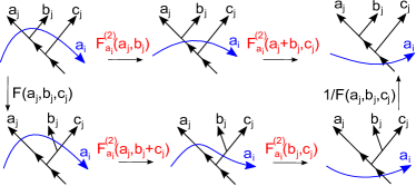
Figure 1: The amplitude of the upper-left configuration can be related to the amplitude of the upper-right configuration in two different ways by the local rule (7). Self-consistency requires the two sequences of operation result in the same linear relations between the amplitudes of the two configurations.

Similarly, to construct a consistent string-net model, we need one more constraint

$$\left|F^{\left(2\right)}\right|=\left|F^{\left(3\right)}\right|=\left|\kappa\right|=1.$$ (20)

This constraint ensures the corresponding exactly soluble Hamiltonians to be Hermitian.

IV.3 Gauge transformation

Like the solution $\{F,d,\alpha,\gamma\}$ to (6), given a solution $\left\{F^{\left(2\right)},\kappa,\eta,F^{\left(3\right)}\right\}$ to the self-consistency conditions (19), we can construct an infinite class of other solutions $\left\{\tilde{F}^{\left(2\right)},\tilde{\kappa},\tilde{\eta},\tilde{F}^{\left(3\right)}\right\}$ by defining

$$\tilde{F}_{a_{i}}^{\left(2\right)}\left(a_{j},b_{j}\right) =F_{a_{i}}^{\left(2\right)}\left(a_{j},b_{j}\right)\frac{f_{a_{i}}\left(a_{j}\right)f_{a_{i}}\left(b_{j}\right)}{f_{a_{i}}\left(a_{j}+b_{j}\right)},$$ (21)

$$\tilde{\kappa}_{a_{i}}\left(a_{j}\right) =\kappa_{a_{i}}\left(a_{j}\right)\frac{f_{a_{i}}\left(a_{j}^{\ast}\right)}{f_{a_{i}}\left(a_{j}\right)},$$

$$\tilde{\eta}_{a_{i}}\left(a_{j}\right) =\eta_{a_{i}}\left(a_{j}\right)\frac{1}{f_{a_{i}}\left(a_{j}\right)^{2}},$$

$$\tilde{F}_{a_{i}}^{\left(3\right)}\left(a_{j},a_{k}\right) =F_{a_{i}}^{\left(3\right)}\left(a_{j},a_{k}\right).$$

Here $f_{a}\left(b\right)$ is any complex function with

$$f_{a}\left(b\right)=f_{b}\left(a\right),\left|f_{a}\left(b\right)\right|=1,f_{a}\left(b\right)=1\text{ if }a\text{ or }b=0.$$

We refer to (21) as the gauge transformations and two sets of solutions $\left\{F^{\left(2\right)},\kappa,\eta,F^{\left(3\right)}\right\}$ and $\left\{\tilde{F}^{\left(2\right)},\tilde{\kappa},\tilde{\eta},\tilde{F}^{\left(3\right)}\right\}$ are called gauge equivalent if they are related by such a transformation. One can show that the gauge transformation can be implemented by a local unitary transformation which can be generated by the time evolution of a local Hamiltonian over a finite period of time. Thus, this implies that if two solutions to the self-consistency conditions (19) are related by a gauge transformation, then the corresponding wave functions $\Phi,\tilde{\Phi}$ describe the same quantum phase. Since we are primarily interested in constructing different topological phases, then we only need to consider one solution to (19) within each gauge equivalence class.

V Intersecting-string-net Hamiltonians

In this section, we will construct a large class of exactly soluble lattice Hamiltonians that have the wave functions $\Phi$ as their ground states. For a given solution $\left\{d,F,\gamma,\alpha\right\}$ and $\left\{F^{\left(2\right)},\kappa,\eta,F^{\left(3\right)}\right\}$ to the self-consistency conditions (6) and (19), we will construct an exactly soluble Hamiltonian whose ground state $\left|\Phi_{latt}\right\rangle$ obeys the local rules (1–3,7–11) on the lattice.

V.1 Definition of the Hamiltonian

Let us first specify the Hilbert space for our model. As the original string-net model is a spin system with the spins located on the links of the honeycomb lattice, the $L$-intersecting string-net model is defined on the $L$ copies of intersecting honeycomb lattices with each flavor of spins living on the links of individual honeycomb lattice. The $L$ honeycomb lattices are arranged in such a way that the $\left(i+1\right)$-th lattice is obtained by shifting the $i$-th lattice by a small constant vector $v$ (see Fig. 2). We assume that the overall shifting between the first and $L$-th honeycomb lattices is smaller than twice the lattice constant $2a$, namely$(L-1)v<2a$ for the sake of ordering the $L$ lattices. The spins of the $i$-th flavor can be $\left|G_{i}\right|$ different states which are labeled by elements of the subgroup $G_{i}:$ $\left\{\left|a_{i}\right\rangle:a_{i}\in G_{i}\right\}$ with $i=1,...,L.$ For the ease of graphical presentation, we replace the honeycomb lattice by a square lattice with the proper lattice splitting at vertices of square lattices in mind (see Fig. 2). As far as the intersections are concerned, intersecting square lattices capture all the intersections on the original intersecting honeycomb lattices and it is more transparent to see the intersections in the square lattices when we consider more intersecting lattices. When a spin of the $i$-th flavor is in state $\left|a_{i}\right\rangle,$ we regard the link as being occupied by a sting of type-$a_{i}$, oriented in a certain direction. If the spin is in state $\left|0\right\rangle,$ the link is occupied by the null string. In this way, each spin state can be equivalently described as an intersecting string-net state.

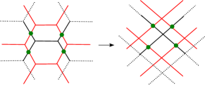
Figure 2: We represent two intersecting honeycomb lattices (on the left) by two intersecting square lattices (on the right) with proper lattice splitting at vertices of square lattices in mind. The green dots denote the intersections between two lattices.

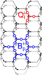
Figure 3: Lattice spin model (22). The $Q_{I}^{i}$ operators act on three spins on the links which meet at vertex $I$ while the $B_{p}^{i}$ operators acts on $12$ spins adjacent to the plaquette $p$ and $4(L-1)$ more spins intersecting $p$ with $L$ being the number of lattices. Here $L=2$ since there are two intersecting honeycomb lattices.

The Hamiltonian is of the form

$$H=-\sum_{i=1}^{L}\left(\sum_{I}Q_{I}^{i}+\sum_{p}B_{p}^{i}\right)$$ (22)

where the first sum runs over all flavors of spins $i=1,...,L$ and the next two sums run over the sites $I$ and the plaquettes $p$ of the $i$-th honeycomb lattice. Here we label the sites and plaquettes of all other lattices according to the ones of the first lattice.

The operator $Q_{I}^{i}$ acts on the 3 spins adjacent to the site $I$ :

$$Q_{I}^{i}\left|\raisebox{-11.56346pt}{\includegraphics[height=28.90755pt]{qi.eps}}\right\rangle=\delta_{a_{i}b_{i}c_{i}}\left|\raisebox{-11.56346pt}{\includegraphics[height=28.90755pt]{qi.eps}}\right\rangle$$

where

$$\delta_{a_{i}b_{i}c_{i}}=\left\{\begin{array}[]{l}1,\text{ if }a_{i}+b_{i}+c_{i}=0\\ 0,\text{ otherwise}\end{array}\right.$$

(see Fig. 3). The $Q_{I}$ terms annihilate the states that do not satisfy the branching rules.

The $B_{p}^{i}$ operator provides dynamics to the string-net configurations. It can be written as a linear combination

$$B_{p}^{i}=\sum_{s_{i}\in G_{i}}a_{s_{i}}B_{p}^{s_{i}},$$

where $B_{p}^{s_{i}}$ describes a $12+4\left(L-1\right)$ spin interaction involving the spins on the $12$ links surrounding the plaquette $p$ and $4$ links of each other $\left(L-1\right)$ honeycomb lattices which intersect of the boundary of the plaquette $p.$ The $B_{p}^{s_{i}}$ operator describes three types of interactions among $L$ flavors of string-nets. First, it contains the 12-spin interaction for each flavor of string-nets. For $L=1$ case, the above Hamiltonian reduces to the original string-net model in Ref. Lin and Levin, 2014. For $L\geq 2,$ it further contains 2-spin interaction at each crossing between any two different flavors of string-nets. The $a_{s_{i}}$ are some complex coefficients satisfying $a_{s_{i}^{\ast}}=a_{s_{i}}^{\ast}.$

The operator $B_{p}^{s_{i}}$ has some special structures. First, it annihilates any state that does not obey the branching rules at 6 vertices surrounding the plaquette $p$. Second, the $B_{p}^{s_{i}}$ acts non-trivially on the 6 inner spins along the boundary of $p$ and it does not affect the outer $6$ spins and other intersecting spins of different flavors. However, its matrix elements depend on the state of outer spins and other intersecting spins of different flavors.

Specifically, the matrix elements are defined by

$$\left\langle\raisebox{-18.06749pt}{\includegraphics[height=43.36243pt]{bp1.eps}}\right|B_{p}^{s_{i}} \left|\raisebox{-18.06749pt}{\includegraphics[height=43.36243pt]{bp2.eps}}\right\rangle$$

$$=B_{p,g_{i}^{\prime}...l_{i}^{\prime}}^{s_{i},g_{i}...l_{i}}\left(a_{i}...f_{i};\sum_{i\neq j}{X_{j}}\right)$$

where

$$B_{p,g_{i}^{{}^{\prime}}...l_{i}^{\prime}}^{s_{i},g_{i}...l_{i}}\left(a_{i}...f_{i};\sum_{i\neq j}\left\{X_{j}\right\}\right)=B_{p,x^{\prime}x}^{s_{i}\left(1\right)}B_{p,x^{\prime}x}^{s_{i}\left(2\right)}B_{p,x^{\prime}x}^{s_{i}\left(3\right)}$$ (23)

with

$$B_{p,x^{\prime}x}^{s_{i}\left(1\right)} =\delta_{g_{i}^{\prime}}^{g_{i}+s_{i}}\delta_{h_{i}^{\prime}}^{h_{i}+s_{i}}\delta_{i_{i}^{\prime}}^{i_{i}+s_{i}}\delta_{j_{i}^{\prime}}^{j_{i}+s_{i}}\delta_{k_{i}^{\prime}}^{k_{i}+s_{i}}\delta_{l_{i}^{\prime}}^{l_{i}+s_{i}}\times$$ (24)

$$F_{s_{i}^{\ast}g_{i}^{\prime}b_{i}}F_{s_{i}^{\ast}h_{i}^{\prime}c_{i}}F_{s_{i}^{\ast}i_{i}^{\prime}d_{i}}F_{s_{i}^{\ast}j_{i}^{\prime}e_{i}}F_{s_{i}^{\ast}k_{i}^{\prime}f_{i}}F_{s_{i}^{\ast}l_{i}^{\prime}a_{i}},$$

$$B_{p,x^{\prime}x}^{s_{i}\left(2\right)} =\prod_{j\neq i}\eta_{s_{i},i_{j}}\frac{F^{(2)}_{g_{j},s_{i}l_{i}}F^{(2)}_{b_{j},s_{i}g_{i}}F^{(2)}_{c_{j},s_{i}i_{i}}\bar{F}^{(2)}_{i_{j},s_{i}j_{i}}}{\bar{F}^{(2)}_{s_{i},g_{j}b_{j}}\bar{F}^{(2)}_{s_{i},(g_{j}+b_{j})c_{j}}},$$ (25)

$$B_{p,x^{\prime}x}^{s_{i}\left(3\right)} =\prod_{j\neq k\neq i}F_{s_{i}}^{\left(3\right)}\left(c_{k}^{*},i_{j}\right)F_{s_{i^{*}}}^{\left(3\right)-1}\left(g_{j},b_{k}\right)$$ (26)

and $F_{abc}\equiv F\left(a,b,c\right),F_{a}^{\left(2\right)}\left(b,c\right)\equiv F_{a,bc}^{\left(2\right)},\eta_{a,b}\equiv\eta_{a}\left(b\right).$ The $g_{i}...l_{i}$ and $a_{i}...f_{i}$ denote $g_{i}h_{i}i_{i}j_{i}k_{i}l_{i}$ and $a_{i}b_{i}c_{i}d_{i}e_{i}f_{i}$ respectively. The $x,x^{\prime}$ denote the spin labels around the plaquette $p$ for the initial and final state configurations, i.e. $x=g_{i}h_{i}\dots$ and $x^{\prime}=g_{i}^{\prime}h_{i}^{\prime}\dots$. Here the action of $B_{p}^{s_{i}}$ is defined to be on the bra state $\left\langle\raisebox{-18.06749pt}{\includegraphics[height=43.36243pt]{bp1.eps}}\right|$ and $\left\{X_{j}\right\}$ in the bra state represents the configuration of other flavors $j\neq i$ of string-nets which intersects the plaquette $p.$ Note that the above expression is only valid if the initial and final states obey the branching rules, i.e. $h_{i}=b_{i}+g_{i},h_{i}^{\prime}=b_{i}+g_{i}^{\prime},$ etc. Otherwise, the matrix element of $B_{p}^{s_{i}}$ vanishes.

The matrix elements of $B_{p}^{s_{i}}$ are the product of three components. The first component $B_{p,x^{\prime}x}^{s_{i}\left(1\right)}$ is the phase factor of creating a closed loop $s_{i}$ on the plaquette $p$ in the absence of other flavors of string-nets. The other two components $B_{p,x^{\prime}x}^{s_{i}\left(2\right)},B_{p,x^{\prime}x}^{s_{i}\left(3\right)}$ are the phase factors associated with the intersections on and inside the plaquette $p$, respectively. They account for the interactions between different flavors of string-nets. The geometry of the intersections of string-nets on and inside the plaquette $p$ is shown in Fig. 4.

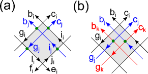
Figure 4: (a) Intersections (green dots) between $i,j$ flavors of strings in the boundary of the plaquette $p$ (the grey region). (b) Intersections between $j,k$ flavors of strings inside the plaquette $p$.

Notice that the above matrix elements are computed for a particular orientation configuration in which the inner links of $i$-th lattice are oriented cyclically and the links of other lattices intersecting the plaquette $p$ are oriented as in Fig. 4. This choice of orientations make the matrix elements simple but however, this orientation configuration can not be extended to the whole lattices while preserving translational symmetry. If we instead choose a translationally invariant orientation configuration as in Fig. 3, the matrix elements are modified as

$$\left\langle\raisebox{-18.06749pt}{\includegraphics[height=43.36243pt]{bp4.eps}}\right|B_{p}^{s_{i}} \left|\raisebox{-18.06749pt}{\includegraphics[height=43.36243pt]{bp5.eps}}\right\rangle$$

$$=\mathbf{B}_{p,g_{i}^{{}^{\prime}}...l_{i}^{\prime}}^{s_{i},g_{i}...l_{i}}\left(a_{i}...f_{i};\sum_{i\neq j}{X_{j}^{t}}\right)$$

with

$$\mathbf{B}_{p,g_{i}^{{}^{\prime}}...l_{i}^{\prime}}^{s_{i},g_{i}...l_{i}} (a_{i}...f_{i};\sum_{i\neq j}\left\{X_{j}^{t}\right\})=B_{p,g_{i}^{{}^{\prime}}...l_{i}^{\prime}}^{s_{i},g_{i}...l_{i}}(a_{i}...f_{i};\sum_{i\neq j}\left\{X_{j}^{t}\right\})$$

$$\times\frac{\alpha_{g_{i}^{*}l_{i}}\alpha_{h_{i}^{\prime}c_{i}}\alpha_{j_{i}^{*}i_{i}}\alpha_{k_{i}^{\prime}f_{i}}\gamma_{g_{i}}\gamma_{i_{i}}\gamma_{k_{i}}}{\alpha_{g_{i}^{\prime*}l_{i}^{\prime}}\alpha_{h_{i}c_{i}}\alpha_{j_{i}^{\prime*}i_{i}^{\prime}}\alpha_{k_{i}f_{i}}\gamma_{g_{i}^{\prime}}\gamma_{i_{i}^{\prime}}\gamma_{k_{i}^{\prime}}}$$

$$\times\frac{\kappa_{l_{i},g_{j}}\kappa_{b_{j},g_{i}^{\prime*}}\kappa_{g_{i}^{\prime*},b_{j}^{*}}\kappa_{c_{j},i_{i}^{\prime*}}\kappa_{s_{i},i_{j}^{*}}\kappa_{j_{i}^{\prime},i_{j}}}{\kappa_{l_{i}^{\prime},g_{j}}\kappa_{b_{j},g_{i}^{*}}\kappa_{g_{i}^{*},b_{j}^{*}}\kappa_{c_{j},i_{i}^{*}}\kappa_{s_{i},i_{j}}\kappa_{j_{i},i_{j}}}.$$ (27)

Here $\{X_{j}^{t}\}$ denotes the translationally invariant orientation configuration of other flavors of string-nets (see Fig. 3). The additional factors come from reversing the orientations on $g_{i},i_{i},k_{i}$ links and gliding $s_{i}$ through vertices involving one null string.

Although the algebraic definition of $B_{p}^{s_{i}}$ is complicated, we provide with an alternative graphical representation for this operator which is much simpler. In the graphical representation, the action of $B_{p}^{s_{i}}$ can be understood as adding a loop of the type-$s_{i}$ string inside the plaquette $p:$

$$\left\langle\raisebox{-18.06749pt}{\includegraphics[height=43.36243pt]{bp1.eps}}\right|B_{p}^{s_{i}}=\left\langle\raisebox{-18.06749pt}{\includegraphics[height=43.36243pt]{bp3.eps}}\right|$$

To obtain matrix elements of $B_{p}^{s_{i}},$ it requires two steps. The first step is to use the local rules (7–11) to glide the string $s_{i}$ to near the boundary of the plaquette. The second step is then to use (1–3) to fuse the string $s_{i}$ onto the links along the boundary of the plaquette. We obtain the phase factors $B_{p,x^{\prime}x}^{s_{i}\left(2\right)}$ and $B_{p,x^{\prime}x}^{s_{i}\left(3\right)}$ in the first step and $B_{p,x^{\prime}x}^{s_{i}\left(1\right)}$ in the second step. In appendix B, we show that this prescription reproduces the formula in equation (23).

V.2 Properties of the Hamiltonian

The Hamiltonian has many nice properties. The first property is that the Hamiltonian is Hermitian if $a_{s_{i}^{\ast}}=a_{s_{i}}^{\ast}.$ This result follow from the identity

$$\left(B_{p}^{s_{i}}\right)^{\dagger}=B_{p}^{s_{i}^{\ast}}.$$

We derive this equality in appendix D.

The second property is that the $Q_{I}^{i}$ and $B_{p}^{s_{i}}$ operators commute with each other:

$$\left[Q_{I_{1}}^{i},Q_{I_{2}}^{j}\right]=0,\quad\left[Q_{I}^{i},B_{p}^{s_{j}}\right]=0,\quad\left[B_{p_{1}}^{s_{i}},B_{p_{2}}^{t_{j}}\right]=0.$$

The first two equalities can be shown easily from the definition of $Q_{I}^{i},B_{p}^{s_{i}}.$ The proof of the third equality is given in appendix C.

Since every term in the Hamiltonian (22) commutes with one another, the model is exactly soluble for any value of the coefficients $a_{s_{i}}.$ In particular, we choose

$$a_{s_{i}}=\frac{d_{s_{i}}}{\left|G_{i}\right|}.$$

With this choice of $a_{s_{i}},$ the $Q_{I}^{i}$ and $B_{p}^{i}$ are projector operators which have eigenvalues $0,1$. It is easy to derive the result for $Q_{I}^{i};$ we show $B_{p}^{i}$ are projector operators in appendix D.

As a result, we can derive the low energy properties of $H$. Let $\left|\left\{q_{I}^{i},b_{p}^{i}\right\}\right\rangle$ denote the simultaneous eigenvalues of $\left\{Q_{I}^{i},B_{p}^{i}\right\}$ with $i=1,..,L:$

$$Q_{I}^{i}\left|\left\{q_{I}^{i},b_{p}^{i}\right\}\right\rangle = q_{I}^{i}\left|\left\{q_{I}^{i},b_{p}^{i}\right\}\right\rangle,$$

$$B_{p}^{i}\left|\left\{q_{I}^{i},b_{p}^{i}\right\}\right\rangle = b_{p}^{i}\left|\left\{q_{I}^{i},b_{p}^{i}\right\}\right\rangle.$$

The corresponding energies are

$$E=-\sum_{i=1}^{L}\left(\sum_{I}q_{I}^{i}+\sum_{p}b_{p}^{i}\right).$$

Since $q_{I}^{i},b_{p}^{i}$ take values in $0$ or $1,$ thus the ground state(s) have $q_{I}^{i}=b_{p}^{i}=1,$ while the excited states have $q_{I}^{i}=0$ or $b_{p}^{i}=0$ for at least one site $I$ or plaquette $p.$ We see that there is a finite energy gap separating the ground states(s) from the excited states. All that remains is to determine the ground state degeneracy. The degeneracy is simply the product of the degeneracy associated with each flavor of string-nets. The degeneracy depends on the global topology of our system. For a disk geometry with open boundary conditions, there is a unique state with $q_{I}^{i}=b_{p}^{i}=1.$ On the other hand, for a periodic torus geometry, the number of degenerate ground states is equal to the number of quasiparticles types (see Ref. Lin and Levin, 2014 for the computation of the ground state degeneracy).

The final property of our model is that the ground state of lattice model in a disk geometry, $|\Phi_{latt}\rangle$, obeys the local rules (1–3) and (7–11). We establish this property in appendix (D). As a result, we conclude that $|\Phi_{latt}\rangle$ is identical to the continuum wave function $\Phi$ restricted to the string-net configurations on the lattice. From now on, we will use $|\Phi\rangle$ to denote both the lattice ground state and the continuum wave function.

VI Quasiparticle excitations

In this section, we discuss the topological properties of the quasiparticle excitations of the string-net Hamiltonian (22). We generalize the analysis in Ref. Lin and Levin, 2014 to multiple flavors of string-nets. We first find all the topologically distinct types of quasiparticles by constructing the string operators which create the quasiparticle excitations. Then we compute their braiding statistics by the commutation algebra of the string operators.

VI.1 String operator picture

For the topological phases, the excitations with nontrivial statistics are generally created by string-like operators. For each topologically distinct quasiparticle excitation $\alpha,$ there is a corresponding string operator $W_{\alpha}\left(P\right)$ where $P$ is the path along which the string operator acts. If $P$ is an open path, then $W_{\alpha}\left(P\right)$ is called an open string operator while if $P$ is a closed path, then $W_{\alpha}\left(P\right)$ is called an closed string operator.

The string operator $W_{\alpha}\left(P\right)$ has several properties. First, an open string operator acting on the ground state $\left|\Phi\right\rangle$ will create an excited state containing a pair of quasiparticle $\alpha$ and its antiparticle at two ends of $P$

$$W_{\alpha}\left(P\right)\left|\Phi\right\rangle=\left|\Phi_{ex}\right\rangle.$$

Furthermore, the excited state does not depend on the path of the string but only on the end points of $P,$ that is

$$W_{\alpha}\left(P\right)\left|\Phi\right\rangle=W_{\alpha}\left(P^{\prime}\right)\left|\Phi\right\rangle$$

for any two paths $P,P^{\prime}$ that have the same end points. Finally, a closed string operator does not create any excitations: $W_{\alpha}\left(P\right)\left|\Phi\right\rangle$ $\propto\left|\Phi\right\rangle$ .

Physically, one may think of an open string operator as describing a process of creating a particle-antiparticle pair out of the ground state and then bringing the two particles to the two ends of the string. Similarly, a closed string operator describes a process of creating a pair of quasiparticles and then moving one of them around the path of the string all the way to its original position, where it annihilates its partner. Throughout the discussion, we assume that the system is defined in a topologically trivial geometry with a unique ground state.

VI.2 Constructing the string operators

We follow the same strategy as Ref. Lin and Levin, 2014 to construct string operators that create each of the distinct quasiparticle excitations of the Hamiltonian (22). We begin with our ansatz for constructing string operators. The string operators are defined by specifying how $W_{\alpha}\left(P\right)$ acts on each string-net configuration. We describe the action of $W_{\alpha}\left(P\right)$ using a graphical representation and we use the convention that $W_{\alpha}\left(P\right)$ acts on a bra $\left\langle X\right|$. Specifically, when $W_{\alpha}\left(P\right)$ is applied to a string-net state $\left\langle X\right|,$ it adds a dashed string along the path $P$ under the preexisting string-nets:

$$\left\langle\raisebox{-11.56346pt}{\includegraphics[height=28.90755pt]{xconfig.eps}}\right|W\left(P\right)=\left\langle\raisebox{-11.56346pt}{\includegraphics[height=28.90755pt]{xconfig1.eps}}\right|.$$

We then replace the dashed string with a type-$s_{i}$ and replace every crossing using the rules:

$$\left\langle\raisebox{-11.56346pt}{\includegraphics[height=28.90755pt]{stringop3a.eps}}\right| =\omega_{s_{i}}\left(a_{i}\right)\left\langle\raisebox{-11.56346pt}{\includegraphics[height=28.90755pt]{stringop3b.eps}}\right|$$ (28)

$$\left\langle\raisebox{-11.56346pt}{\includegraphics[height=28.90755pt]{stringop4a.eps}}\right| =\bar{\omega}_{s_{i}}\left(a_{i}\right)\left\langle\raisebox{-11.56346pt}{\includegraphics[height=28.90755pt]{stringop4b.eps}}\right|$$ (29)

$$\left\langle\raisebox{-11.56346pt}{\includegraphics[height=28.90755pt]{stringop1a.eps}}\right| =\Omega_{s_{i}}\left(a_{j}\right)\left\langle\raisebox{-11.56346pt}{\includegraphics[height=28.90755pt]{stringop1b.eps}}\right|,$$ (30)

$$\left\langle\raisebox{-11.56346pt}{\includegraphics[height=28.90755pt]{stringop2a.eps}}\right| =\bar{\Omega}_{s_{i}}\left(a_{j}\right)\left\langle\raisebox{-11.56346pt}{\includegraphics[height=28.90755pt]{stringop2b.eps}}\right|$$ (31)

Here the first two equations specify the rules for crossings between string-nets of the same flavor while the last two equations are rules for crossings between string-nets of different flavors. The $\omega,\bar{\omega},\Omega,\bar{\Omega}$ are four complex-valued functions defined on the group $G$ with $\omega\left(0\right)=\bar{\omega}\left(0\right)=\Omega\left(0\right)=\bar{\Omega}\left(0\right)=1.$ After making these replacements, the resulting state $\left\langle X^{\prime}\right|$ is multiplied by a product of $\omega,\bar{\omega},\Omega,\bar{\Omega}$ and it is simply the matrix element of the string operator $\left\langle X\left|W\left(P\right)\right|X^{\prime}\right\rangle.$ This defines the string operator $W\left(P\right).$

VI.3 Path independence constraints

The string operators $W\left(P\right)$ must satisfy path independence so that they can create deconfined quasiparticle excitations at two ends of the path. Specifically, $W$ satisfies path independence if and only if

$$\left\langle\raisebox{-11.56346pt}{\includegraphics[height=28.90755pt]{string1a.eps}}\middle|\Phi\right\rangle =\left\langle\raisebox{-11.56346pt}{\includegraphics[height=28.90755pt]{string1b.eps}}\middle|\Phi\right\rangle$$ (32)

$$\left\langle\raisebox{-7.22743pt}{\includegraphics[height=16.62178pt]{string2a.eps}}\middle|\Phi\right\rangle =\left\langle\raisebox{-7.22743pt}{\includegraphics[height=16.62178pt]{string2b.eps}}\middle|\Phi\right\rangle$$ (33)

$$\left\langle\raisebox{-11.56346pt}{\includegraphics[height=28.90755pt]{string3a.eps}}\middle|\Phi\right\rangle =\left\langle\raisebox{-11.56346pt}{\includegraphics[height=28.90755pt]{string3b.eps}}\middle|\Phi\right\rangle$$ (34)

$$\left\langle\raisebox{-4.33601pt}{\includegraphics[height=13.00806pt]{string4a.eps}}\middle|\Phi\right\rangle =\left\langle\raisebox{-4.33601pt}{\includegraphics[height=13.00806pt]{string4b.eps}}\middle|\Phi\right\rangle$$ (35)

$$\left\langle\raisebox{-11.56346pt}{\includegraphics[height=28.90755pt]{string5a.eps}}\middle|\Phi\right\rangle =\left\langle\raisebox{-11.56346pt}{ \includegraphics[height=28.90755pt]{string5b.eps}}\middle|\Phi\right\rangle$$ (36)

Other deformations of the path can be built out of these elementary ones. These graphical relations can be translated into algebraic conditions by using the local rules (1–3,7–11). The result is

$$\mathbf{w}_{s_{i}}\left(a_{i}\right)\mathbf{w}_{s_{i}}\left(b_{i}\right) =c_{s_{i}}\left(a_{i},b_{i}\right)\mathbf{w}_{s_{i}}\left(a_{i}+b_{i}\right),$$ (37a)

$$\mathbf{\bar{w}}_{s_{i}}\left(a_{i}\right) =\mathbf{w}_{s_{i}}\left(a_{i}\right)^{-1},$$ (37b)

$$\Omega_{s_{i}}\left(a_{j}\right)\Omega_{s_{i}}\left(b_{j}\right) =F_{s_{i}}^{\left(2\right)}\left(a_{j},b_{j}\right)\Omega_{s_{i}}\left(a_{j}+b_{j}\right),$$ (37c)

$$\bar{\Omega}_{s_{i}}\left(a_{j}\right) =\Omega_{s_{i}}\left(a_{j}\right)^{-1}\eta_{s_{i}}\left(a_{j}\right),$$ (37d)

$$\Omega_{s_{i}}\left(a_{j}\right)\Omega_{s_{i}}\left(a_{k}\right) =F_{s_{i}}^{\left(3\right)}\left(a_{j},a_{k}\right)\Omega_{s_{i}}\left(a_{k}\right)\Omega_{s_{i}}\left(a_{j}\right).$$ (37e)

Here we define

$$\mathbf{w}_{s_{i}}\left(a_{i}\right) =\omega_{s_{i}}\left(a_{i}\right)F\left(s_{i},a_{i},a_{i}^{\ast}\right),$$

$$\mathbf{\bar{w}}_{s_{i}}\left(a_{i}\right) =\bar{\omega}_{s_{i}}\left(a_{i}\right)F\left(a_{i},s_{i},s_{i}^{\ast}\right),$$

$$c_{s_{i}}\left(a_{i},b_{i}\right) =\frac{F\left(a_{i},b_{i},s_{i}\right)F\left(s_{i},a_{i},b_{i}\right)}{F\left(a_{i},s_{i},b_{i}\right)}.$$ (38)

Notice that (37a,37b), (37c,37d), (37e) involve one, two and three flavors of strings respectively. The string operators constructed by the first two rules (37a,37b) were studied in Ref. Lin and Levin, 2014.

To solve (37a–37e), we note that the self-consistency condition (6) implies that $c_{s_{i}}\left(a_{i},b_{i}\right)$ obey the identity

$$c_{s_{i}}\left(a_{i},b_{i}\right)c_{s_{i}}\left(a_{i}+b_{i},c_{i}\right)=c_{s_{i}}\left(b_{i},c_{i}\right)c_{s_{i}}\left(a_{i},b_{i}+c_{i}\right).$$ (39)

This identity resembles the self-consistency condition (19a) for $F_{s_{i}}^{\left(2\right)}\left(a_{j},b_{j}\right)$. The only difference is that $c_{s_{i}}\left(a_{i},b_{i}\right)$ is associated with one flavor of string-nets while $F_{a_{i}}^{\left(2\right)}\left(a_{j},b_{j}\right)$ is associated with two different flavors of string-nets. Eqs. (38,19a) are also called the 2-cocycle condition. They are the factor systems of a projective representationChen et al. (2013). Thus, solving (37a,37c) is equivalent to finding a projective representation corresponding to the factor systems $c_{s_{i}}\left(a_{i},b_{i}\right)$ and $F_{a_{i}}^{\left(2\right)}\left(a_{j},b_{j}\right)$ respectively. Furthermore, one can see from (37e) that if $F_{s_{i}}^{\left(3\right)}\left(a_{j},a_{k}\right)$ is nontrivial, then $\Omega_{s_{i}}\left(a_{j}\right)$ require to be higher dimensional objects, namely matrices.

VI.4 Unifying different flavors of strings

So far in our construction, different flavors of strings cross but do not branch with one another. With this restriction, we obtain several self-consistency conditions (19) and path independence conditions (37). Some equations are similar except they are associated with different flavors of strings. For the ease of solving this set of equations, we like to first compactify them to a fewer equations.

To this end, we combine different flavors of string labels into a vector $a=(a_{1},\dots,a_{i},\dots,a_{L})$, namely we regard the flavor index $i$ as the $i$-th component of the vector $a$. In this way, we equivalently unify all different flavors of strings $a_{i}\in G_{i}$ into one flavor of strings with multiple components $a\in G=\prod_{i=1}^{L}G_{i}$. We relabel the strings by $L$-component vectors $a$. The strings can branch if each component satisfies the corresponding component-wise branch rules, namely $(a,b,c)$ is allowed if $a_{i}+b_{i}+c_{i}=0$ for all components $i$.

After unifying the flavors of strings, $F,F^{(2)}$ can now take different components of $a$ as inputs, e.g. $F^{(2)}_{a_{i}}(a_{j},a_{k})$. Moreover, all strings can branch. To implement this in our construction, we do the replacement at each crossing:

$$\left\langle\raisebox{-10.11775pt}{\includegraphics[height=25.29494pt]{crossinga.eps}}|\Phi\right\rangle=\left\langle\raisebox{-15.17719pt}{\includegraphics[height=32.52127pt]{crossingb.eps}}|\Phi\right\rangle.$$ (40)

Namely, each crossing is understood as fusing two strings and then splitting it into two with exchanged order. Intuitively, one can think of this replacement as zooming in the crossing where $a_{j},a_{k}$ branch and split. As a consequence of this replacement in the local rules (7–11), one can relate the parameters $F,F^{(2)},\kappa,\eta,F^{(3)}$ and reduce the number of independent parameters.

Specifically, applying (40) to (11) gives the condition

$$F_{s_{i}}^{\left(3\right)}\left(a_{j},a_{k}\right)=\frac{F_{s_{i}}^{\left(2\right)}\left(a_{j},a_{k}\right)}{F_{s_{i}}^{\left(2\right)}\left(a_{k},a_{j}\right)}.$$ (41)

Similarly, by inserting (40) to the local rules (7–10), one can obtain

$$F^{(2)}_{a_{i}}(a_{j},b_{j}) =\frac{F(a_{i},a_{j},a_{j}^{*})F(a_{i},b_{j},b_{j}^{*})}{F(a_{i},a_{j}+b_{j},(a_{j}+b_{j})^{*})c_{a_{i}}(a_{j},b_{j})}$$ (42)

$$\kappa_{a_{i}}(a_{j}) =F(a_{j}^{*},a_{i},a_{j})F(a_{j}^{*},a_{i}+a_{j},a_{i}^{*})$$ (43)

$$\eta_{a_{i}}(a_{j}) =1/(F(a_{i},a_{j},a_{j}^{*})F(a_{j},a_{i},a_{i}^{*})).$$ (44)

Since the parameters $F^{(2)},\kappa,\eta,F^{(3)}$ are functions of $F$, then solving (19) reduces to solve (6) with the strings labeled by the group $G=\prod_{i}G_{i}$.

Furthermore, one can insert (41–42) into (37) and simplify the expressions by (6). We can then combine the conditions (37) into

$$\mathbf{w}_{s}\left(a\right)\mathbf{w}_{s}\left(b\right) =c_{s}\left(a,b\right)\mathbf{w}_{s}\left(a+b\right),$$ (45)

$$\mathbf{\bar{w}}_{s}\left(a\right) =\mathbf{w}_{s}\left(a\right)^{-1},$$

$$c_{s}\left(a,b\right) =\frac{F\left(a,b,s\right)F\left(s,a,b\right)}{F\left(a,s,b\right)},$$ (46)

with

$$\mathbf{w}_{s_{i}}(a_{i})=\mathbf{w}_{s}(a)\text{ with }s=s_{i},a=a_{i},$$

$$\Omega_{s_{i}}(a_{j})=\frac{F(s,a,a^{*})}{\mathbf{w}_{s}(a)}\text{ with }s=s_{i},a=a_{j}.$$

Again, $s,a,b$ are elements of the group $G.$

Thus, by unifying the flavors of strings and applying (40) to each crossing of intersecting string-nets in our construction, we successfully reduce the equations (19) and (37) into the equations (6) and (45) with strings labeled by $G=\prod_{i}G_{i}$. The last two are exactly the equations which determines ground state wave functions and string operators in the original construction in Ref. Lin and Levin, 2014. Therefore, we establish the equivalence between our new construction associated with multiple flavors of strings labeled by $\{G_{i},i=1,\dots,L\}$ and the original construction associated with one flavor of strings labeled by $G=\prod_{i=1}^{L}G_{i}$.

In the rest of the discussion, we stick to the convention that string-nets of different flavors cross one another with the understanding that the crossings are resolved by (40). The convention, namely using $F^{(2)},F^{(3)}$, simplifies the description of the string-net states and models since $F^{(2)},F^{(3)}$ are complicated combinations of $F$ (see Eqs. (42,41)). In the next section, we will analyze the string operators parametrized by $\mathbf{w}_{s}$ in Eq. (45).

VI.5 Solving (45) for the string parameters $\mathbf{w}$

We want to find all complex valued functions $\mathbf{w}$ that satisfy (45). It is sufficient to find $\mathbf{w}$ satisfying (45), $\mathbf{\bar{w}}$ can be obtained immediately from (49). There are two cases to consider: $c_{s}\left(a,b\right)$ is symmetric in $a,b$ or it is non-symmetric. First, if $c_{s}\left(a,b\right)$ is symmetric, Eq. (45) has scalar solutions. It was solved in Ref. Lin and Levin, 2014 in great details so we will not repeat the computation but only cite some relevant results for completeness. The resulting particles in this case are abelian quasiparticles. If $c_{s}\left(a,b\right)$ is non-symmetric, we can see that  Eq. $\left(\ref{string0}\right)$ has no nonzero scalar solutions, since the left-hand side is manifestly symmetric in $a,b$ while the right-hand side is non-symmetric. To build a path independent string operator, we have to allow the parameters $\mathbf{w}$ to be matrices rather than scalars.  Therefore, we need to look for higher dimensional projective representations with factor system $c_{s}\left(a,b\right).$ The resulting particles have non-abelian statistics.

Let’s first review the case with symmetric $c_{s}\left(a,b\right).$ We assume that the group is $G=\prod_{i=1}^{L}\mathbb{Z}_{N_{i}}.$ Let $e_{1},...,e_{L}$ be the generators of $G.$ Once we find the values of $\mathbf{w}_{s}\left(e_{i}\right)$ for each generator $e_{i},$ then $\mathbf{w}_{s}$ is fully determined by Eq. $\left(\ref{string0}\right).$ To find the values of $\mathbf{w}_{s}\left(e_{i}\right),$ we set $a=e_{i}$ and $b=ye_{i}$ with integer $y$ in (45) and take the product of the equation over $y=0,1,...,N_{i}-1.$ By using the fact $N_{i}e_{i}=0,$ we find

$$\mathbf{w}_{s}\left(e_{i}\right)^{N_{i}}=\prod_{y=0}^{N_{i}-1}c_{s}\left(e_{i},ye_{i}\right).$$ (47)

We can see that $\mathbf{w}_{s}\left(e_{i}\right)$ can take $N_{i}$ different values for each $i.$ Thus, there are $\prod_{k}N_{k}=\left|G\right|$ solutions to Eq $\left(\ref{ws}\right)$ for a given $s.$ The parameter $s$ can also take $\left|G\right|$ different values, so altogether we find $\left|G\right|^{2}$ solutions, corresponding to $\left|G\right|^{2}$ path independent string operators. When we apply them to the ground state, they will create quasiparticles at two ends of the string. Thus, the above operators allow us to construct $\left|G\right|^{2}$ different quasiparticle excitations.

Now, we consider the case with non-symmetric $c_{s}\left(a,b\right)$. Again, we fix $s=\left(s_{1},s_{2},...,s_{L}\right)$ and set $a=e_{j},b=e_{k}.$ (Let us remind that $s,a,b$ are $L$-component vectors and the subindex $i$ denotes the $i$-th component.) Once we find the value of $\mathbf{w}_{s}\left(e_{i}\right)$, then $\mathbf{w}_{s}\left(a\right)$ is fully determined by equation (45). To proceed, it is useful to define the ratio

$$C_{s}\left(e_{j},e_{k}\right)=\frac{c_{s}\left(e_{j},e_{k}\right)}{c_{s}\left(e_{k},e_{j}\right)}.$$ (48)

When $C_{s}=1,$ namely $c_{s}\left(a,b\right)$ is symmetric, $\mathbf{w}_{s}$ has one dimensional representation as discussed above. If $C_{s}\neq 1,$ $\mathbf{w}_{s}$ has higher dimensional representation as we now discuss. Thus, we can rewrite $\left(\ref{string0}\right)$ as

$$\mathbf{w}_{s}\left(e_{j}\right)\mathbf{w}_{s}\left(e_{k}\right)=C_{s}\left(e_{j},e_{k}\right)\mathbf{w}_{s}\left(e_{k}\right)\mathbf{w}_{s}\left(e_{j}\right).$$ (49)

By the fact that $C_{s}\left(e_{j},e_{k}\right)$ is antisymmetric in $e_{j},e_{k}$ (see Eq. (48)) and the linearity in $s$, we can further parametrize $C_{s}\left(e_{i},e_{j}\right)$ by

$$C_{s}\left(e_{j},e_{k}\right)=\exp\left(2\pi i\sum_{i}\frac{s_{i}p_{ijk}}{N_{ijk}}\right)$$

where $p_{ijk}$ is an antisymmetric tensor taking values in $0,1,...,N_{ijk}$ with $N_{ijk}$ being the great common divisor of $N_{i},N_{j},N_{k}.$

Next, for a given $s$, we consider a fixed set of $\left\{s_{i}p_{ijk}\text{ with }i,j,k=1,...,L\right\}$. Let $N$ be the least common multiple of the set $\left\{N_{ijk}\text{ with }i,j,k=1,...,L\right\}$. We then rewrite

$$C_{s}\left(e_{j},e_{k}\right)=\exp\left(2\pi i\frac{t_{jk}}{N}\right)$$ (50)

with $t_{jk}=\sum_{i}\frac{N}{N_{ijk}}s_{i}p_{ijk}$ being the elements of the $L\times L$ antisymmetric integer matrix $T=\left[t_{jk}\right].$ We can diagonalize $T$ into a skew-normal form by a unimodular integer matrix $U,$ i.e. $\left|\det U\right|=1:$

$$T=UDU^{T}$$ (51)

with

$$D=\left(\begin{array}[]{cc}0&D_{1}\\ -D_{1}&0\end{array}\right)\oplus...\oplus\left(\begin{array}[]{cc}0&D_{s}\\ -D_{s}&0\end{array}\right)\oplus 0_{L-2s}.$$ (52)

Here $0_{L-2s}$ is an $\left(L-2s\right)\times\left(L-2s\right)$ null matrix.

One nice thing about the skew-normal form (51) is that it allows us to obtain the projective representations associated with the factor set (50) from the ones with the diagonal factor set $exp(2\pi iD_{jk}/N)$ where $D_{jk}$ are the matrix elements of the block-diagonal matrix $D$ in (52)Jagannathan (1985). More specifically, once we find the representation of $\left\{\mathbf{w}_{s}^{\prime}\left(e_{i}\right),i=1,...,L\right\}$ which obeys

$$\mathbf{w}_{s}^{\prime}\left(e_{j}\right)\mathbf{w}_{s}^{\prime}\left(e_{k}\right)=\exp\left(2\pi i\frac{D_{jk}}{N}\right)\mathbf{w}_{s}^{\prime}\left(e_{k}\right)\mathbf{w}_{s}^{\prime}\left(e_{j}\right)$$ (53)

with $D_{jk}$ being the $jk$-th element of $D,$ the representation of $\left\{\mathbf{w}_{s}\left(e_{i}\right),i=1,...,L\right\}$ which obey $\left(\ref{string01}\right)$

$$\mathbf{w}_{s}\left(e_{j}\right)\mathbf{w}_{s}\left(e_{k}\right)=\exp\left(2\pi i\frac{t_{jk}}{N}\right)\mathbf{w}_{s}\left(e_{k}\right)\mathbf{w}_{s}\left(e_{j}\right)$$

can be obtained by taking the product of $\mathbf{w}^{\prime}_{s}$:

$$\mathbf{w}_{s}\left(e_{i}\right)=c_{i}^{{}^{\prime}}\mathbf{w}_{s}^{\prime}\left(e_{1}\right)^{u_{i1}}\mathbf{w}_{s}^{\prime}\left(e_{2}\right)^{u_{i2}}...\mathbf{w}_{s}^{\prime}\left(e_{L}\right)^{u_{iL}},i=1,...,L.$$ (54)

Here $c_{i}$ are proper complex scalars chosen such that $\mathbf{w}_{s}\left(e_{i}\right)^{N_{i}}=I$ and $u_{ij}=\left[U\right]_{ij}.$

All that remains is to determine the representation of $\left\{\mathbf{w}_{s}^{\prime}\left(e_{i}\right),i=1,...,L\right\}$ obeying (53). To this end, let us first look at the pair $\left\{\mathbf{w}_{s}^{\prime}\left(e_{2l-1}\right),\mathbf{w}_{s}^{\prime}\left(e_{2l}\right)\right\}$ with $l=1,...,s$ which obey

$$\mathbf{w}_{s}^{\prime}\left(e_{2l-1}\right)\mathbf{w}_{s}^{\prime}\left(e_{2l}\right)=\exp\left(2\pi i\frac{D_{l}}{N}\right)\mathbf{w}_{s}^{\prime}\left(e_{2l}\right)\mathbf{w}_{s}^{\prime}\left(e_{2l-1}\right).$$

The pair $\left\{\mathbf{w}_{s}^{\prime}\left(e_{2l-1}\right),\mathbf{w}_{s}^{\prime}\left(e_{2l}\right)\right\}$ can be represented by the shift $S_{l}$ and clock $C_{l}$ matrices with dimension

$$d_{l}=\frac{N}{\gcd\left(D_{l},N\right)}.$$

Here the shift $S_{l}$ and clock $C_{l}$ matrices are

$$S_{l}=\left(\begin{array}[]{ccccc}0&1&0&...&0\\ 0&0&1&...&0\\ 0&0&...&1&0\\ ...&...&...&...&...\\ 1&0&0&...&0\end{array}\right),C_{l}=\left(\begin{array}[]{ccccc}1&0&0&...&0\\ 0&\omega&0&...&0\\ 0&0&\omega^{2}&...&0\\ ...&...&...&...&0\\ 0&0&0&...&\omega^{d_{l}-1}\end{array}\right)$$ (55)

with $\omega=\exp\left(\frac{2\pi i}{d_{l}}\right).$ Since the matrix $D$ has the block diagonal form (53), the full representation of $\left\{\mathbf{w}_{s}^{\prime}\left(e_{i}\right),i=1,...,L\right\}$ can be expressed as

$$\mathbf{w}_{s}^{\prime}\left(e_{2l-1}\right)=I_{1}\otimes...\otimes I_{l-1}\otimes C_{l}\otimes I_{l+1}\otimes...\otimes I_{s},$$

$$\qquad\mathbf{w}_{s}^{\prime}\left(e_{2l}\right)=I_{1}\otimes...\otimes I_{l-1}\otimes S_{l}\otimes I_{l+1}\otimes...\otimes I_{s},$$

$$\qquad\qquad\qquad\qquad\qquad\qquad\text{ with }l=1,...,s,$$

$$\mathbf{w}_{s}^{\prime}\left(e_{m}\right)=I_{1}\otimes...\otimes I_{s},\text{ with }m>2s.$$

Here $I_{l}$ is the $d_{l}\times d_{l}$ identity matrix. Thus, the dimension of the representation $\left\{\mathbf{w}_{s}^{\prime}\left(e_{i}\right),i=1,...,L\right\}$ is

$$d_{s}=\prod_{l=1}^{s}d_{l}=\frac{N^{s}}{\prod_{i=1}^{s}\gcd\left(D_{l},N\right)}.$$

Finally, Plugging $\left\{\mathbf{w}_{s}^{\prime}\left(e_{i}\right),i=1,...,L\right\}$ to (54), we then obtain the representation of $\left\{\mathbf{w}_{s}\left(e_{i}\right),i=1,...,L\right\}.$ This completes the solution to the equation (45).

After constructing all the string operators and thus all the quasiparticle excitations, we now discuss the labeling scheme for quasiparticle excitations. We label each type-$s$ solution $\mathbf{w}_{s}$ to Eqs. (45) by an ordered pair $\alpha=\left(s,m\right)$ where $s\in G$ and $m$ is the representation of $G.$ We denote this solution by $\mathbf{w}_{\alpha}$, the corresponding string operator by $W_{\alpha}$ and the quasiparticle excitation created by $W_{\alpha}$ as $\alpha.$ We will also call the $\left(s,0\right)$ excitations “fluxes” and the $\left(0,m\right)$ excitations “charges” (The definition of the pure fluxes $\left(s,0\right)$ is a matter of convention.). Likewise, we think of a general excitation $\left(s,m\right)$ as a composite of a flux and a charge.

VI.6 Braiding statistics of quasiparticles

In the previous section, we constructed string operators $W_{\alpha}$ for each quasiparticle excitation $\alpha=\left(s,m\right)$ where $s\in G$ and $m$ is a representation of $G$. In this section, we will compute the braiding statistics of these quasiparticles. We first review the computation of the exchange statistics $\theta_{\alpha}$ for every particle $\alpha$ and the mutual statistics $\theta_{\alpha\beta}$ for every pair of quasiparticles $\alpha,\beta$ in the abelian topological phases. We then compute the braiding statistics of the non-abelian quasiparticle excitations.

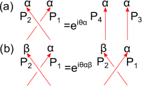
Figure 5: (a) Computation of exchange statistics $e^{i\theta_{\alpha}}$ of quasiparticle $\alpha$ created by $W_{\alpha}.$ (b) Computation of mutual statistics $e^{i\theta_{\alpha\beta}}$ between two quasiparticles created by $W_{\alpha},W_{\beta}.$

To begin, we review the general relationship between braiding statistics and the string operator algebra in the abelian topological phases. Let $\alpha,\beta$ be two abelian quasiparticles and let $W_{\alpha},W_{\beta}$ be the corresponding string operators. Then the exchange statistics $\theta_{\alpha}$ can be extracted from the algebra

$$W_{\alpha}\left(P_{2}\right)W_{\alpha}\left(P_{1}\right)\left|\Phi\right\rangle=e^{i\theta_{\alpha}}W_{\alpha}\left(P_{4}\right)W_{\alpha}\left(P_{3}\right)\left|\Phi\right\rangle$$

for any four paths $P_{1},P_{2},P_{3},P_{4}$ with the geometry of Fig. 5(a) and $\left|\Phi\right\rangle$ denotes the ground state of the system. By the path independence conditions and the local rules, one can show that

$$e^{i\theta_{\alpha}}=\mathbf{w}_{\alpha}\left(s\right).$$ (56)

On the other hand, the mutual statistics between two excitations $\alpha=\left(a,m\right),\beta=\left(t,n\right)$ are encoded in the algebra (see Fig. 5(b))

$$W_{\beta}\left(P_{2}\right)W_{\alpha}\left(P_{1}\right)\left|\Phi\right\rangle=e^{i\theta_{\alpha\beta}}W_{\alpha}\left(P_{1}\right)W_{\beta}\left(P_{2}\right)\left|\Phi\right\rangle.$$

In the same way, one can find that

$$e^{i\theta_{\alpha\beta}}=\mathbf{w}_{\beta}\left(s\right)\mathbf{w}_{\alpha}\left(t\right).$$ (57)

Thus, in the abelian topological phases, $\left(\ref{exstat}\right),\left(\ref{mutualstat1}\right)$ allow us to compute the quasiparticle braiding statistics after we solve $\mathbf{w}_{\alpha}$ in Eq. $\left(\ref{string0}\right).$

Next, we compute the braiding statistics of particles in the non-abelian topological phases. The computation of braiding statistics is similar as in the abelian case. However, in this case, the string parameters $\mathbf{w}_{\alpha}$ are matrices. Thus, in order to extract the statistics phases, we need to consider the whole braiding path (instead of segments of the braiding path for the abelian phases) to contract the matrix indices.

The exchange statistics can be computed by comparing the two braiding processes. In the first process, we create a pair of quasiparticles $\alpha,\bar{\alpha},$ exchange them and then annihilate the pair. In the second process, we create them and annihilate the pair without exchange. The ratio of the amplitudes for the two processes define the exchange statistics:

$$e^{i\theta_{\alpha}}=\frac{Tr\left[\mathbf{w}_{\alpha}\left(s\right)\right]}{\dim\left(\alpha\right)}$$ (58)

with $\dim\left(\alpha\right)$ being the dimension of the representation $\alpha.$

To describe the mutual statistics of two particles $\alpha=\left(s,\alpha\right),\beta=\left(t,\beta\right),$ which is the matrix element $s_{\alpha\beta}$ of the S matrix, we consider the following process: We create two pairs of quasiparticles $\alpha,\bar{\alpha},\beta,\bar{\beta},$ braid $\alpha$ around $\beta$ and then annihilate the two pairs. The amplitude of this process divided by a factor $\left|G\right|$ defines the matrix element $s_{\alpha\beta}$ of the S matrix. More specifically, we have

$$s_{\alpha\beta}=\frac{\left\langle\Phi\left|\raisebox{-11.56346pt}{\includegraphics[height=28.90755pt]{sab.eps}}\right|\Phi\right\rangle}{\left|G\right|}=\frac{Tr\left(\mathbf{w}_{\alpha}\left(t\right)\right)Tr\left(\mathbf{w}_{\beta}\left(s\right)\right)}{\left|G\right|}.$$ (59)

One can see that (58,59) reduce to (56,57) respectively for abelian quasiparticles $\alpha$ with $dim(\alpha)=1$ up to some normalization constants.

VII QUASIPARTICLE STATISTICS OF GENERAL ABELIAN STRING-NET MODELS

After discussing the general framework for constructing multiple flavors of abelian string-net models and computing the quasiparticle braiding statistics, in this section we explicitly compute the braiding statistics of these abelian string-net models. First, we review the string-net models with one flavor of strings labeled by $a\in G=\mathbb{Z}_{N}.$ Then we analyze the general case $G=\mathbb{Z}_{N_{1}}\times...\times\mathbb{Z}_{N_{L}}$ where the models consist of $L$ flavors of strings, each of which is labeled by $a_{i}\in G_{i}=\mathbb{Z}_{N_{i}}.$

VII.1 $\mathbb{Z}_{N}$ string-net models

We begin by reviewing the abelian string-net models with group $G=\mathbb{Z}_{N}.$ In the $\mathbb{Z}_{N}$ models, the string type $a$ has values in $\left\{0,1,...,N-1\right\}.$ The dual string type is defined by $a^{\ast}=-a$ $\left(\text{mod }N\right),$ while the allowed branchings are the triplets $\left(a,b,c\right)$ that satisfy $a+b+c=0$ $\left(\text{mod }N\right).$

There are $N$ distinct solutions to the self-consistency conditions $\left(\ref{sfeqa}\right)$ parametrized by $p=0,...,N-1:$

$$F\left(a,b,c\right) =e^{2\pi i\frac{pa}{N^{2}}\left(b+c-\left[b+c\right]\right)},$$ (60)

$$d_{a} =1,\gamma_{a}=F\left(a^{\ast},a,a^{\ast}\right),$$

$$\alpha\left(a,b\right) =F\left(a,b,\left(a+b\right)^{\ast}\right)\gamma_{a+b}.$$

The arguments $a,b,c$ can take values in the range $0,1,...,N-1$ and the square bracket $\left[b+c\right]$ denotes $b+c\left(\text{mod }N\right)$ with values also taken in the range $0,1,...,N-1.$ For each of the above $N$ solutions, we can construct a corresponding string-net model.

Next, we compute the braiding statistics of the quasiparticle excitations in these models. By inserting the solution (60) to $\left(\ref{string0}\right),$ we find

$$c_{s}\left(a,b\right) =e^{2\pi i\frac{ps}{N^{2}}\left(a+b-\left[a+b\right]\right)},$$

$$\mathbf{w}_{\left(s,m\right)}\left(a\right) =e^{2\pi i\left(\frac{psa}{N^{2}}+\frac{ma}{N}\right)}.$$

Then, the exchange statistics $\left(\ref{exstat}\right)$ of $\alpha=\left(s,m\right)$ is given by

$$\theta_{\left(s,m\right)}=2\pi\left(\frac{ps^{2}}{N^{2}}+\frac{ms}{N}\right)$$

and the mutual statistics $\left(\ref{mutualstat1}\right)$ of $\alpha=\left(s,m\right)$ and $\beta=\left(t,n\right)$ is

$$\theta_{\left(s,m\right)\left(t,n\right)}=2\pi\left(\frac{2pst}{N^{2}}+\frac{ns+mt}{N}\right).$$

VIII $\mathbb{Z}_{N_{1}}\times...\times\mathbb{Z}_{N_{k}}$ string-net models

We now construct the string-net models with $G=\mathbb{Z}_{N_{1}}\times...\times\mathbb{Z}_{N_{L}}$. These models were constructed previously in Ref. Lin and Levin, 2014. Here we construct the models in a different way. We think of the models consisting of $L$ flavors of string-nets. Each flavor of string-nets form a $\mathbb{Z}_{N_{i}}$ string-net model as reviewed in the previous section. The strings of each flavor are labeled by $a_{i}\in\mathbb{Z}_{N_{i}}$ and the dual string is defined by $a_{i}^{\ast}=-a_{i}$ $\left(\text{mod }N_{i}\right).$ Each flavor of string-nets satisfies the branching rules $a_{i}+b_{i}+c_{i}=0$ $\left(\text{mod }N_{i}\right)$ for $i=1,...,L$.

As in the $\mathbb{Z}_{N}$ case discussed above, we have to find distinct solutions to the self-consistency conditions (6,19). This problem is closely related to the problem of computing the cohomology group $H^{3}\left(\prod_{i}\mathbb{Z}_{N_{i}},U\left(1\right)\right).$ This cohomology group has been calculated previouslyPropitius (1995); Chen et al. (2013, 2013) and is given by

$$H^{3}\left(\prod_{i}\mathbb{Z}_{N_{i}},U\left(1\right)\right)=\prod_{i}\mathbb{Z}_{N_{i}}\prod_{i<j}\mathbb{Z}_{N_{ij}}\prod_{i<j<k}\mathbb{Z}_{N_{ijk}}$$ (61)

where $N_{ij}$ denotes the greatest common divisor of $N_{i}$ and $N_{j},$ and similarly for $\mathbb{Z}_{N_{ijk}}.$

In Ref. Lin and Levin, 2014, they focused on realizing the abelian topological phases and only discussed the $\prod_{i}\mathbb{Z}_{N_{i}}\prod_{i<j}\mathbb{Z}_{N_{ij}}$ distinct solutions and constructed the corresponding abelian string-net models. In this paper, we will find all distinct solutions including those realizing the non-abelian topological phases. Before going to the details, it is worth mentioning that our new construction provides a geometric interpretation of these distinct solutions. Specifically, Eq. $\left(\ref{h3}\right)$ can be understood by thinking of the multiple flavors of string-nets, each of which is associated with $G_{i}=\mathbb{Z}_{N_{i}}.$ There are $N_{i}$ distinct string-net models corresponds to $N_{i}$ distinct solutions $F_{i}\left(a_{i},b_{i},c_{i}\right)$ and altogether we have $\prod_{i}N_{i}$ distinct decoupled string-net models. Now we allow these string-net models to intersect with one another. We need additional local rules (7–11) to specify how they intersect. There are two kinds of intersections to consider. One is intersections associated with each two flavors of strings, which we will call 2-intersections and the other is the intersections associated with three flavors of strings, which we will call 3-intersections. As we will show later, there are $\prod_{i<j}N_{ij}$ distinct solutions $F_{a_{i}}^{\left(2\right)}\left(a_{j},b_{j}\right)$ for 2-intersections and $\prod_{i<j<k}N_{ijk}$ distinct solutions $F_{a_{i}}^{3}\left(a_{j},b_{k}\right)$ for 3-intersections. Putting everything together, we find all the solutions to the self-consistency conditions and can be used to construct $\mathcal{N}=\prod_{i}N_{i}$ $\prod_{i<j}N_{ij}\prod_{i<j<k}N_{ijk}$ distinct string-net models which realize $\mathcal{N}$ distinct topological phases.

More explicitly, the solutions to the self-consistency conditions (6,19) are (for a particular gauge choice)

$$F_{i}\left(a_{i},b_{i},c_{i}\right) =e^{2\pi i\frac{p_{i}a_{i}}{N_{i}^{2}}\left(b_{i}+c_{i}-\left[b_{i}+c_{i}\right]_{i}\right)},$$ (62)

$$d_{a_{i}} =1,\gamma_{a_{i}}=F_{i}\left(a_{i}^{\ast},a_{i},a_{i}^{\ast}\right),$$

$$\alpha_{i}\left(a_{i},b_{i}\right) =F\left(a_{i},b_{i},\left(a_{i}+b_{i}\right)^{\ast}\right)\gamma_{a_{i}+b_{i}},$$

$$F_{a_{i}}^{\left(2\right)}\left(b_{j},c_{j}\right) =e^{2\pi ia_{i}\frac{p_{ij}}{N_{i}N_{j}}\left(b_{j}+c_{j}-\left[b_{j}+c_{j}\right]_{j}\right)},$$

$$\kappa_{a_{i}}\left(b_{j}\right) =e^{2\pi ia_{i}\frac{p_{ij}}{N_{i}N_{j}}\left(b_{j}+\left[b_{j}^{*}\right]_{j}\right)},$$

$$\eta_{a_{i}}\left(b_{j}\right) =1,$$

$$F_{a_{i}}^{\left(3\right)}\left(b_{j},c_{k}\right) =e^{2\pi i\frac{p_{ijk}}{N_{ijk}}a_{i}b_{j}c_{k}}.$$

Here $p$ has values in $0,1,..,N_{i}$, $p_{ij}$ has values in $0,1,..,N_{ij}$ if $i<j$ and $p_{ij}=0$ if $i>j$ (Namely, we can gauge away the solutions with $p_{ij},i>j$.) and $p_{ijk}$ is an antisymmetric tensor with the element of $p_{ijk}$ taking values in $0,1,...,N_{ijk}$. The square bracket $\left[b_{i}+c_{i}\right]_{i}$ denotes $\left(b_{i}+c_{i}\right)$ $\left(\text{mod }N_{i}\right).$ As promised, there are $\prod_{i}N_{i}$ distinct $F_{i}\left(a_{i},b_{i},c_{i}\right),$ $\prod_{i<j}N_{ij}$ distinct $F_{a_{i}}^{\left(2\right)}\left(a_{j},b_{j}\right)$ and $\prod_{i<j<k}N_{ijk}$ distinct $F_{a_{i}}^{3}\left(a_{j},b_{k}\right)$ parametrized by $p,p_{ij}$ and $p_{ijk}.$

For comparison, in the original construction, the strings are labeled by elements of $G$ parametrized by $L$-component integer vectors $a=\left(a_{1},a_{2},...,a_{L}\right)$ where $0\leq a_{i}\leq N_{i}-1.$ The solutions to the self-consistency conditions $\left(\ref{sfeqa}\right)$ are

$$F\left(a,b,c\right) =e^{2\pi i\sum_{ij}\frac{P_{ij}a_{i}}{N_{i}N_{j}}\left(b_{j}+c_{j}-\left[b_{j}+c_{j}\right]_{j}\right)+2\pi i\sum_{ijk}\frac{p_{ijk}}{N_{ijk}}a_{i}b_{j}c_{k}}$$ (63)

$$d_{a} =1,\gamma_{a}=F\left(a^{\ast},a,a^{\ast}\right),$$

$$\alpha\left(a,b\right) =F\left(a,b,\left(a+b\right)^{\ast}\right)\gamma_{a+b}.$$

Here $F$ is parametrized by the matrix $P_{ij}$ and the antisymmetric tensor $p_{ijk}.$ The matrix $P_{ij}$ is a $L\times L$ upper-triangular integer matrix with diagonal elements $P_{ii}=p$ and off diagonal elements $P_{ij}=p_{ij}.$There are also $\mathcal{N}$ distinct solutions parametrized by $P_{ij}$ and $p_{ijk}.$

It is now obvious that (62) encodes the same information as (63) as discussed in section VI.4. In this regard, our new model can be viewed as an alternative construction of the original model while the new model provides a clear geometric picture of internal structure of the original construction. In general, our construction provides various ways of building lattice models which realize topological order $G$ by different ways of encoding the information of $F(a,b,c)$ with $a,b,c\in G$, namely different decomposition of $G$.

The $\mathcal{N}$ solutions can be used to construct $\mathcal{N}$ different lattice models (22). Our next task is to determine the braiding statistics of the quasiparticle excitations in these models. To this end, we can insert the solution $\left(\ref{sol3}\right)$ to (45) and find $\mathbf{w}_{s}.$ After obtaining $\mathbf{w}_{s},$ the braiding statistics are given by (58,59). Instead of giving the explicitly expression for the braiding statistics of quasiparticles (we will compute the braiding statistics explicitly in the example section), we want to make connection with the topological invariants defined in Ref. Wang and Levin, 2015. The topological invariants are a set of three gauge invariant quantities $\left\{\Theta_{i},\Theta_{ij},\Theta_{ijk}\right\}$ associated with various braiding processes of excitations with unit flux. Let $e_{i}$ denote the excitation which carries a unit flux $\frac{2\pi}{N_{i}}$ associate $i$-th flavor of string-nets. More explicitly, $\Theta_{i}$ is $N_{i}$ times of exchange statistics of $e_{i};$ $\Theta_{ij}$ is $N^{ij}$ times of mutual statistics of $e_{i},e_{j}$ with $N^{ij}$ being the least common multiple of $N_{i},N_{j}$ and $\Theta_{ijk}$ is the phase associated with braiding $e_{i}$ around $e_{j}$, then around $e_{k},$ then around $e_{j}$ in an opposite direction and finally around $e_{k}$ in an opposite direction. Then, the three topological invariants can be expressed in terms of $c,F^{\left(2\right)}$ and $F^{\left(3\right)}:$

$$e^{i\Theta_{i}} =\prod_{y=0}^{N_{i}-1}c_{e_{i}}\left(e_{i},ye_{i}\right),$$

$$e^{i\Theta_{ij}} =\prod_{y=0}^{N^{ij}-1}F_{e_{i}}^{\left(2\right)}\left(e_{j},ye_{j}\right)F_{e_{j}}^{\left(2\right)}\left(e_{i},ye_{i}\right),$$

$$e^{i\Theta_{ijk}} =F_{e_{i}}^{\left(3\right)}\left(e_{j},e_{k}\right).$$

One can check the quantities on the right hand side are indeed invariant under the gauge transformations. Thus, $\mathcal{N}$ topological phases are characterized by distinct topological invariants and therefore they belong to distinct quantum phases.

IX Relation between different constructions

We have constructed the multi-flavor string-net model by intersecting different flavors of string-net models, each of which is associated with $G_{i}.$ We show that the new model realizes the same topological order as the original model with group $G=\prod_{i}G_{i}$. This suggests that there are many ways of constructing models to realize the same topological phases with $G$ by intersecting string-net models with different choices of subgroups of $G$. In this section, we will discuss the equivalence of these construction from a mathematical point of view.

We recall that in the original string-net models with group $G=\prod_{i}\mathbb{Z}_{N_{i}},$ there are $|H^{3}\left(G,U(1)\right)|$ distinct solutions to the 3-cocycle conditions (6) and thus there are $|H^{3}\left(G,U(1)\right)|$ models which realize distinct topological phases. On the other hand, in the new construction, we construct multiple flavors of intersecting string-net models, each of which belong to a group $G_{i}=\mathbb{Z}_{N_{i}}.$ In this way, we have to solve not only the 3-cocycle conditions $\left(\ref{sfeqa}\right)$ for each flavor of strings but also the 2-cocycle conditions $\left(\ref{sfeq1}\right)$ and 1-cocycle conditions $\left(\ref{sfeq5}\right).$ Correspondingly, there are $\prod_{i}\mathbb{Z}_{N_{i}}$ distinct solutions to $\left(\ref{sfeqa}\right),$ $\prod_{i<j}\mathbb{Z}_{N_{ij}}$ distinct solutions to $\left(\ref{sfeq1}\right)$ and $\prod_{i<j<k}\mathbb{Z}_{N_{ijk}}$ distinct solutions to $\left(\ref{sfeq5}\right)$ as parametrized by $p,p_{ij},p_{ijk}$ in $\left(\ref{sol2}\right),$ respectively. Thus, the two constructions give rises to the same number of distinct topological phases.

It turns out that the relation between the two constructions of string-net models are described by the mathematical relation called the Künneth formula. In $d$ spatial dimension, given a group $G=G_{1}\times G_{2},$ the Künneth formula is given by

$$H^{d+1}\left(G,U(1)\right)=\sum_{k=0}^{d+1}H^{k}\left(G_{1},H^{d+1-k}\left(G_{2},U\left(1\right)\right)\right).$$ (64)

The formula expresses the cohomology group with $G$ in $d+1$ dimension in terms of cohomology groups with its subgroups $G_{1},G_{2}$ in the lower dimensions. Assuming the distinct topological phases with group $G$ in $d$ spatial dimension is classified by $H^{d+1}\left(G,U(1)\right)$ and interpreting $H^{k}$ as dictating various rules for $\left(d-k\right)$-intersections among $\left(d-1\right)$-dimensional objects, then the formula suggests how to construct models which realize $d$ dimensional topological phases with $G$ by intersecting some simpler models which realize topological phases with its subgroups $G_{1},G_{2}$. Notice that $G_{1},G_{2}$ can be arbitrary two subgroups of $G$ such that $G=G_{1}\times G_{2}$. For different choices of $G_{1},G_{2}$, we have different decomposition of $H^{d+1}(G,U(1))$ which corresponds to intersecting models associated with different $G_{1},G_{2}$. All these constructions give rise to the same topological phases classified by $H^{d+1}(G,U(1))$. In this paper, we demonstrate the case with $d=2$ and $G=\prod_{i}G_{i}$ with $G_{i}=\mathbb{Z}_{N_{i}}$.

Let use consider $G=\mathbb{Z}_{N_{1}}\times\mathbb{Z}_{N_{2}}\times\mathbb{Z}_{N_{3}}$ and $d=2$ for example. We can choose $G=G_{1}\times G_{2}$ with $G_{1}=\mathbb{Z}_{N_{1}}$ and $G_{2}=\mathbb{Z}_{N_{2}}\times\mathbb{Z}_{N_{3}}.$ Applying the Künneth formula, we get

$$H^{3}\left(G,U\left(1\right)\right) = H^{3}\left(\mathbb{Z}_{N_{1}},U\left(1\right)\right)+H^{3}\left(\mathbb{Z}_{N_{2}}\times\mathbb{Z}_{N_{3}},U\left(1\right)\right)$$

$$+H^{2}\left(\mathbb{Z}_{N_{1}},\mathbb{Z}_{N_{2}}\times\mathbb{Z}_{N_{3}}\right)+H^{1}\left(\mathbb{Z}_{N_{1}},\mathbb{Z}_{N_{23}}\right).$$

On the left hand side, it corresponds to the original string-net construction with group $G$ and the model realizes $H^{3}\left(G,U\left(1\right)\right)$ distinct phases. On the right hand side, there are four components. The first two terms counts the distinct phases realized by two non-intersecting string-net models, which we call $G_{1}$-model and $G_{2}$-model. The last two terms counts the additional distinct phases which arise from the intersections between the $G_{1}$-model and the $G_{2}$-model. Different rules for 2-intersections give $H^{2}\left(\mathbb{Z}_{N_{1}},\mathbb{Z}_{N_{2}}\times\mathbb{Z}_{N_{3}}\right)=\mathbb{Z}_{N_{12}}+\mathbb{Z}_{N_{13}}$ distinct phases while different rules for the 3-intersections give $H^{1}\left(\mathbb{Z}_{N_{1}},\mathbb{Z}_{N_{23}}\right)=\mathbb{Z}_{N_{123}}$ distinct phases. Totally, the intersecting models gives $|H^{3}(G,U(1))|$ distinct quantum phases. Alternatively, one can choose $G_{1}=\mathbb{Z}_{N_{1}}\times\mathbb{Z}_{N_{2}}$ and $G_{2}=\mathbb{Z}_{N_{3}}$ and get different models which realize these topological phases.

Furthermore, the Künneth formula shows that the information of $F(a,b,c)\in H^{3}(G,U(1))$ with $G=\prod_{i}G_{i}$ can be encoded in some simpler objects $F(a_{i},b_{i},c_{i}),F^{(2)}_{a_{i}}(a_{j},b_{j}),F^{(3)}_{a_{i}}(a_{j},a_{k})$ where $a_{i}\in G_{i}$ and $F^{(2)},F^{(3)}$ satisfy simpler algebraic conditions (19a,19f). This is explicitly shown in Eqs. (41,42). Thus, our construction concretely demonstrates the Künneth formula in building lattice models.

It is worth mentioning the other interesting application of the Künneth formula is the decorated domain wall construction in Ref. Chen et al., 2014 to realize symmetry protected topological (SPT) phases.  In that paper, they consider the case that $G$ of the form $G=\mathbb{Z}_{2}\times G^{\prime}.$ They proposed that SPT phases with symmetry $G$ in $d$ spatial dimensions can be constructed by first decorating the $\mathbb{Z}_{2}$ domain walls with $d-1$ dimensional SPT phases with symmetry $G^{\prime}$ and then condensing these decorated domain walls. This construction corresponds to $k=1$ term in the Künneth formula $\left(\ref{kformula}\right)$ which can realize $H^{1}\left(\mathbb{Z}_{2},H^{d}\left(G^{\prime},U\left(1\right)\right)\right)$ distinct SPT phases. (In general, $\left(\ref{kformula}\right)$ suggests even more ways to construct models for higher dimensional SPT phases. One can construct $d$ dimensional SPT phases with symmetry $G=G_{1}\times G_{2}$ by decorating $d-k$ dimensional SPT phases with symmetry $G_{2}$ onto $d-k$ dimensional $G_{1}$ symmetry defects and then proliferating the $G_{1}$ symmetry defects.)

In addition, by the duality between SPT phases and topological phasesLevin and Gu (2012), we can ungauge our intersecting string-net models with $G=G_{1}\times G_{2}$ and obtain models which realize SPT phases with symmetry $G.$ However, our construction is different from the decorated domain wall construction in Ref. Chen et al., 2014. The physical picture of our construction is to assign $G_{1}$ charges to the vertices of $G_{2}$ domain walls and assign $G_{2}$ charges to the vertices of $G_{1}$ domain walls (see the rule 7) and then proliferate the $G_{1},G_{2}$ domain walls. A similar idea was proposed in Ref. Gu et al., 2016 to realize SPT phases from the field theory perspectives.

Finally, as suggested by the Künneth formula, our construction can be generalized to non-abelian groups and higher dimensions. We leave the generalization for the future work.

X Examples

In this section, we present some illustrative examples of intersecting string-net models, namely $\mathbb{Z}_{2}\times\mathbb{Z}_{2}$ and $\mathbb{Z}_{2}\times\mathbb{Z}_{2}\times\mathbb{Z}_{2}$ string-net models. For each example, we construct the wave functions and the corresponding Hamiltonian and analyze braiding statistics of quasiparticles.

X.1 $\mathbb{Z}_{2}\times\mathbb{Z}_{2}$ string-net model

We consider $\mathbb{Z}_{2}\times\mathbb{Z}_{2}$ string-nets as two flavors of $\mathbb{Z}_{2}$ string-nets intersecting with one another. In this way, the Hilbert space of the $\mathbb{Z}_{2}\times\mathbb{Z}_{2}$ models involves two string types $\left\{0=\left(0,0\right),b=\left(1,0\right)\right\}$ for the first flavor and the other two string types $\left\{0=\left(0,0\right),r=\left(0,1\right)\right\}$ for the second flavor. Each $\mathbb{Z}_{2}$ string-nets obeys $\mathbb{Z}_{2}$ branching rules.

To construct the wave function and Hamiltonian, we solve the self-consistency conditions for $\{F,d,\gamma,\alpha,F^{(2)},\kappa,\eta\}.$ We use the general solution (62):

$$F\left(b,b,b\right)=\left(-1\right)^{p_{1}},d_{b}=\left(-1\right)^{p_{1}},$$

$$F\left(r,r,r\right)=\left(-1\right)^{p_{2}},d_{r}=\left(-1\right)^{p_{2}},$$

$$F_{b}^{\left(2\right)}\left(r,r\right)=\kappa_{b}\left(r\right)=\left(-1\right)^{p_{12}},$$

$$\text{other }F,F^{\left(2\right)},d,\gamma,\alpha,\eta,\kappa=1.$$

Here $p_{1},p_{2},p_{12}=0,1.$ The $p_{i}=0$ solution corresponds to the toric code model while the $p_{i}=1$ solution corresponds to the double semion model for the $i$-th flavor of string-nets with $i=1,2$. The $p_{12}=0,1$ solutions indicate if two flavors of string-nets are decoupled or coupled. Altogether there are $8$ distinct phases for $\mathbb{Z}_{2}\times\mathbb{Z}_{2}$ string-net models: each flavor of string-nets realizes two distinct phases and two different ways of intersections between them realize two more phases.

The toric code and double semion models are well studied in Ref. Levin and Wen, 2005. Here we will focus on the new phases from the intersections. For simplicity, we consider the model with $p_{1}=p_{2}=0,$ namely two intersecting toric code models. Then the $p_{12}=0$ solution corresponds to two decoupled Toric code models while the $p_{12}=1$ solution gives the other interesting model as we will construct.

The nontrivial local rules for the $p_{12}=1$ case are given by

$$\Phi\left(\raisebox{-11.56346pt}{\includegraphics[height=28.90755pt]{ex1rule1a.eps}}\right)=-\Phi\left(\raisebox{-11.56346pt}{\includegraphics[height=28.90755pt]{ex1rule1b.eps}}\right),$$

$$\Phi\left(\raisebox{-7.22743pt}{\includegraphics[height=23.12692pt]{ex1rule2a.eps}}\right)=-\Phi\left(\raisebox{-7.22743pt}{\includegraphics[height=23.12692pt]{ex1rule2b.eps}}\right).$$

The ground state consists of closed blue and red loops and their intersections. The wave function, namely the solution for the local rules, is

$$\Phi\left(X\right)=\left(-1\right)^{N_{ij}\left(X\right)}.$$

Here $N_{ij}$ is the total number of red null strings inside the blue loops.

The model is made up of two species of spins: blue spins $\sigma_{i}$ and red spins $\tau_{i}.$ The blue spins $\sigma_{i}$ live on the links $i$ of square lattice while the red spins $\tau_{i}$ live on the link $i$ of the shifted square lattice. We regard a link with $\sigma_{i}^{x}=-1$ as being occupied by a blue string and the state $\sigma_{i}^{x}=1$ as being unoccupied. Similarly, if $\tau_{i}^{x}=-1$ then $i$ is occupied by a red string while if $\tau_{i}^{x}=1$, then $i$ is empty. The Hamiltonian is of the form

$$H=-\sum_{I}Q_{I}^{b}-\sum_{I}Q_{I}^{r}-\sum_{p}B_{p}^{b}-\sum_{p}B_{p}^{r}$$ (65)

with

$$Q_{I}^{b} =\frac{1}{2}\left(1+\prod_{i\in I}\sigma_{i}^{x}\right),Q_{I}^{r}=\frac{1}{2}\left(1+\prod_{i\in I}\tau_{i}^{x}\right),$$

$$B_{p}^{b} =\frac{1}{2}\left(1+\prod_{i\in\{1,2,5,6\}}\sigma_{i}^{z}\left(-1\right)^{\frac{1-\tau_{1}^{x}}{2}\frac{1-\tau_{5}^{x}}{2}+\frac{1-\tau_{2}^{x}}{2}\frac{1-\tau_{6}^{x}}{2}}\right),$$

$$B_{p}^{r} =\frac{1}{2}\left(1+\prod_{i\in\{1,2,3,4\}}\tau_{i}^{z}\left(-1\right)^{\sum_{i\in\left\{1,2,3,4\right\}}\frac{1-\sigma_{i}^{x}}{2}\frac{1-\tau_{i}^{x}}{2}}\right).$$

The link indices are labeled as in Fig. 6.

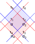
Figure 6: The schematic lattice for the model (65). The lattice contains two intersecting square lattices with blue $\sigma$ and red $\tau$ spins sitting on the links of each lattice.

Next we compute the quasiparticle excitations for the above Hamiltonian. Each flavor of spins realize a toric code model which has four distinct quasiparticles: $\left\{1_{i},e_{i},m_{i},e_{i}m_{i}\right\}$ with $i=b,r$ where $1_{i}$ is trivial quasiparticle, $e_{i}$ is the charge excitation, $m_{i}$ is the magnetic flux excitation and $e_{i}m_{i}$ is the bound state of $e_{i}$ and $m_{i}$. The $e_{i}m_{i}$ particle is a fermion and any two distinct nontrivial quasiparticles have semionic mutual braiding statistics. What is left is to determine the mutual statistics between quasiparticles of different flavors. By (57), we find that

$$\theta_{e_{1}e_{2}} =0,\quad\theta_{e_{1}m_{2}}=0,\quad\theta_{m_{1}e_{2}}=0,$$

$$\theta_{e_{1}m_{1}} =\pi,\quad\theta_{e_{2}m_{2}}=\pi,\quad\theta_{m_{1}m_{2}}=\frac{\pi}{2}.$$

Other mutual statistics can be determined by linearity of the statistical phases.

The 8 distinct $\mathbb{Z}_{2}\times\mathbb{Z}_{2}$ string-net models are parametrized by $p_{1},p_{2},p_{12}=0,1.$ Each of the models has $4\times 4=16$ quasiparticles, which can be labeled by ordered pairs $\left(s_{1},s_{2},m_{1},m_{2}\right)$ with $s_{i},m_{i}=0,1.$ These quasiparticle statistics can be described by four component $U\left(1\right)$ Chern-Simons theory with $K$ matrix

$$K=\left(\begin{array}[]{cccc}0&0&2&0\\ 0&0&0&2\\ 2&0&-2p_{1}&-p_{12}\\ 0&2&-p_{12}&-2p_{2}\end{array}\right).$$

X.2 $\mathbb{Z}_{2}\times\mathbb{Z}_{2}\times\mathbb{Z}_{2}$ string-net model

Our next example is the $\mathbb{Z}_{2}\times\mathbb{Z}_{2}\times\mathbb{Z}_{2}$ string-net model. The corresponding Chern-Simons theory with $G=\mathbb{Z}_{2}\times\mathbb{Z}_{2}\times\mathbb{Z}_{2}$ was studied in Ref. Propitius, 1995 and He et al., 2016. In this section, we will construct the ground state wave function and the lattice model. Then we analyze the quasiparticle braiding statistics. The model is interesting because they can realize the topological phase with non-abelian quasiparticles.

The Hilbert space for the $\mathbb{Z}_{2}\times\mathbb{Z}_{2}\times\mathbb{Z}_{2}$ string-net models involves three flavors of strings, each of which has two string types labeled by $\left\{0_{i},1_{i}\right\}$ with flavor index $i=1,2,3$. These strings are self-dual and obey $\mathbb{Z}_{2}$ branching rules.

To construct the Hamiltonians and wave functions for the $\mathbb{Z}_{2}\times\mathbb{Z}_{2}\times\mathbb{Z}_{2}$ string-net models, we solve the self-consistency conditions (6,19) for $\left\{F,d,\gamma,\alpha,F^{\left(2\right)},F^{\left(3\right)},...\right\}.$ The general solution (62) tells us that there are $2^{3}\times 2^{3}\times 2=128$ solutions labeled by $p_{i},p_{ij},p_{ijk}=0,1.$ The first factor $2^{3}$ means that each flavor of string-nets can be in toric code or double semion models. The second factor $2^{3}$ means that there can be nontrivial intersections among any two flavors of string-nets which give new topological phases as discussed in the previous example. The last factor $2$ indicates that there is one additional new phase which results from a nontrivial intersections among three flavors of string-nets.

In this example, we will mainly focus on the last new phase, namely the phase corresponding to $p_{i}=p_{ij}=0$ and $p_{ijk}=1.$ In this case, the only nontrivial local rule is given by

$$\Phi\left(\raisebox{-11.56346pt}{\includegraphics[height=28.90755pt]{ex2rule1a.eps}}\right)=-\Phi\left(\raisebox{-11.56346pt}{\includegraphics[height=28.90755pt]{ex2rule1b.eps}}\right).$$

The ground state wave function is

$$\Phi\left(X\right)=\left(-1\right)^{N_{ijk}\left(X\right)}$$

for any closed string-net configuration $X$. Here $N_{ijk}\left(X\right)$ is the number of crossings between two of the three flavors $i,j$ of strings inside the loops of the third flavor $k$. Notice that $N_{ijk},N_{jki},N_{kij}$ have the same parity. Thus, to count $N_{ijk}(X)$, we can choose any one flavor of loops and count the number of crossings of the other two flavors of strings inside the loops. For example, let $X=\left(\raisebox{-11.56346pt}{\includegraphics[height=28.90755pt]{nijk.eps}}\right)$. Then $N_{123}(X)=3$ because there are 3 1-2-crossings in the 3-loop. Similarly, one can see $N_{231}(X)=N_{312}(X)=1$. Thus they have the same parity.

Next, we want to construct the Hamiltonian. The model is made up of three flavors of spins: 1-spins $\sigma_{i}$, 2-spins $\tau_{i}$ and 3-spins $\mu_{i}.$ The three kinds of spins live on the links $i$ of three square lattices as shown in Fig. 7. Again, if $\sigma_{i}^{x}=-1,$ then $i$ is occupied by a 1-string while if $\sigma_{i}^{x}=1$, then $i$ is empty. Similarly for the 2-spins $\tau_{i}$ and 3-spin $\mu_{i}.$ The Hamiltonian is of the form

$$H=\sum_{i=1,2,3}\left(-\sum_{I}Q_{I}^{i}-\sum_{p}B_{p}^{i}\right)$$ (66)

with

$$Q_{I}^{1} =\frac{1}{2}\left(1+\prod_{i\in I}\sigma_{i}^{x}\right),Q_{I}^{2}=\frac{1}{2}\left(1+\prod_{i\in I}\tau_{i}^{x}\right),$$

$$Q_{I}^{3} =\frac{1}{2}\left(1+\prod_{i\in I}\mu_{i}^{x}\right),$$

$$B_{p}^{1} =\frac{1}{2}\left(1+\prod_{i\in p}\sigma_{i}^{z}\left(-1\right)^{f\left(\tau_{3}^{x},\mu_{4}^{x}\right)+f\left(\tau_{4}^{x},\mu_{3}^{x}\right)}\right),$$

$$B_{p}^{2} =\frac{1}{2}\left(1+\prod_{i\in p}\tau_{i}^{z}\left(-1\right)^{f\left(\sigma_{2}^{x},\mu_{3}^{x}\right)+f\left(\sigma_{1}^{x},\mu_{4}^{x}\right)}\right),$$

$$B_{p}^{3} =\frac{1}{2}\left(1+\prod_{i\in p}\mu_{i}^{z}\left(-1\right)^{f\left(\sigma_{1}^{x},\tau_{2}^{x}\right)+f\left(\sigma_{2}^{x},\tau_{1}^{x}\right)}\right).$$

Here we define

$$f\left(a,b\right)=\frac{1-a}{2}\frac{1-b}{2}.$$

The phase factors associated with $B_{p}^{i}$ terms count the number of crossings of the two $j,k$ flavors of strings inside the plaquette $p$ of the $i$-lattice with $i\neq j\neq k$ (see Fig. 7).

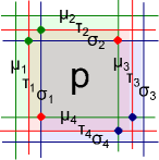
Figure 7: The schematic lattice for the model (66). The lattice contains three intersecting square lattices with three types of spins sitting on the links of each lattice.

Now, we compute the braiding statistics of quasiparticles. Recall that we label the quasiparticles by $\alpha=\left(s,m\right)$ where $s$ is the group element of $G=\mathbb{Z}_{2}\times\mathbb{Z}_{2}\times\mathbb{Z}_{2}$ and $m$ is the representation of $\mathbf{w}.$ We will label $s=\left(s_{1},s_{2},s_{3}\right)\equiv s_{1}s_{2}s_{3}$ with $s_{1},s_{2},s_{3}=0,1.$

To proceed, we use the general solution

$$F\left(a,b,c\right) =\exp\left(i\pi\left(\begin{array}[]{c}a_{1}b_{2}c_{3}+b_{1}c_{2}a_{3}+c_{1}a_{2}b_{3}\\ -a_{1}c_{2}b_{3}-b_{1}a_{2}c_{3}-c_{1}b_{2}a_{3}\end{array}\right)\right),$$

$$c_{s}\left(a,b\right) =\exp\left(i\pi\left(\begin{array}[]{c}s_{1}a_{2}b_{3}+a_{1}b_{2}s_{3}+b_{1}s_{2}a_{3}\\ -s_{1}b_{2}a_{3}-a_{1}s_{2}b_{3}-b_{1}a_{2}s_{3}\end{array}\right)\right).\text{ }$$

Inserting the solution to (45), we can then solve the string parameters $\mathbf{w}_{s}\left(a\right).$ Let $e_{1}=100,e_{2}=010,e_{3}=001$ be the generators of $G.$ To find $\mathbf{w}_{s}\left(a\right),$ it is sufficient to solve $\mathbf{w}_{s}\left(e_{1}\right),\mathbf{w}_{s}\left(e_{2}\right),\mathbf{w}_{s}\left(e_{3}\right)$ and $\mathbf{w}_{s}\left(a\right)$ can be obtained from $\left(\ref{string0}\right).$

There are four cases to consider. First, when $s=000,$ $c_{0}\left(a,b\right)=1$ and thus the string parameter is one dimensional representation of $G$ parametrized by integer $m_{1},m_{2},m_{3}=0,1:\mathbf{w}_{\left(0,m_{1}m_{2}m_{3}\right)}\left(a\right)=\exp\left(\pi i\left(m_{1}a_{1}+m_{2}a_{2}+m_{3}a_{3}\right)\right)$. The corresponding particles are charges which are bosons.

The second case is when $s\in\left\{100,010,001\right\}.$ In particular, $\mathbf{w}_{100}$ satisfies

$$\mathbf{w}_{100}\left(e_{1}\right)^{2}=\mathbf{w}_{100}\left(e_{2}\right)^{2}=\mathbf{w}_{100}\left(e_{3}\right)^{2}=I,$$

$$\left[\mathbf{w}_{100}\left(e_{2}\right),\mathbf{w}_{100}\left(e_{3}\right)\right]_{+}=0,$$

$$\left[\mathbf{w}_{100}\left(e_{2}\right),\mathbf{w}_{100}\left(e_{1}\right)\right]_{-}=0,$$

$$\left[\mathbf{w}_{100}\left(e_{3}\right),\mathbf{w}_{100}\left(e_{1}\right)\right]_{-}=0,$$

Here $I$ is a $2\times 2$ identity matrix and $\left[\mathbf{w}_{s}\left(a\right),\mathbf{w}_{s}\left(b\right)\right]_{\pm}=\mathbf{w}_{s}\left(a\right)\mathbf{w}_{s}\left(b\right)\pm\mathbf{w}_{s}\left(b\right)\mathbf{w}_{s}\left(a\right)$. One can find two inequivalent two dimensional representations for $\mathbf{w}_{\left(100,\pm\right)}$ labeled by $\pm$:

$$\mathbf{w}_{\left(100,\pm\right)}\left(e_{1}\right)=\pm I,\mathbf{w}_{\left(100,\pm\right)}\left(e_{2}\right)=\sigma_{x},\mathbf{w}_{\left(100,\pm\right)}\left(e_{3}\right)=\sigma_{z}.$$

Similarly, for $s=010,001,$ one can find

$$\mathbf{w}_{\left(010,\pm\right)}\left(e_{1}\right) =\sigma_{z},\mathbf{w}_{\left(010,\pm\right)}\left(e_{2}\right)=\pm I,\mathbf{w}_{\left(010,\pm\right)}\left(e_{3}\right)=\sigma_{x},$$

$$\mathbf{w}_{\left(001,\pm\right)}\left(e_{1}\right) =\sigma_{x},\mathbf{w}_{\left(001,\pm\right)}\left(e_{2}\right)=\sigma_{z},\mathbf{w}_{\left(001,\pm\right)}\left(e_{3}\right)=\pm I.$$

The third case is when $s\in\left\{110,101,011\right\}.$ Let’s first consider $\mathbf{w}_{110}$ which satisfies

$$\mathbf{w}_{110}\left(e_{1}\right)^{2}=\mathbf{w}_{110}\left(e_{2}\right)^{2}=\mathbf{w}_{110}\left(e_{3}\right)^{2}=I,$$

$$\left[\mathbf{w}_{110}\left(e_{2}\right),\mathbf{w}_{110}\left(e_{3}\right)\right]_{+}=0,$$

$$\left[\mathbf{w}_{110}\left(e_{1}\right)\mathbf{w}_{110}\left(e_{3}\right)\right]_{+}=0,$$

$$\left[\mathbf{w}_{110}\left(e_{1}\right),\mathbf{w}_{110}\left(e_{2}\right)\right]_{-}=0.$$

Then $\mathbf{w}_{\left(110,\pm\right)}$ can be represented by

$$\mathbf{w}_{\left(110,\pm\right)}\left(e_{1}\right)=\sigma_{x},\mathbf{w}_{\left(110,\pm\right)}\left(e_{2}\right)=\pm\sigma_{x},\mathbf{w}_{\left(110,\pm\right)}\left(e_{3}\right)=\sigma_{z}.$$

In the same manner, we can find

$$\mathbf{w}_{\left(101,\pm\right)}\left(e_{1}\right) =\pm\sigma_{x},\mathbf{w}_{\left(101,\pm\right)}\left(e_{2}\right)=\sigma_{z},\mathbf{w}_{\left(101,\pm\right)}\left(e_{3}\right)=\sigma_{x},$$

$$\mathbf{w}_{\left(011,\pm\right)}\left(e_{1}\right) =\sigma_{z},\mathbf{w}_{\left(011,\pm\right)}\left(e_{2}\right)=\sigma_{x},\mathbf{w}_{\left(011,\pm\right)}\left(e_{3}\right)=\pm\sigma_{x}.$$

Finally, when $s=111,\mathbf{w}_{111}$ satisfies

$$\mathbf{w}_{111}\left(e_{1}\right)^{2}=I,\mathbf{w}_{111}\left(e_{2}\right)^{2}=I,\mathbf{w}_{111}\left(e_{3}\right)^{2}=I,$$

$$\left[\mathbf{w}_{111}\left(e_{1}\right),\mathbf{w}_{111}\left(e_{2}\right)\right]_{+}=0,$$

$$\left[\mathbf{w}_{111}\left(e_{1}\right),\mathbf{w}_{111}\left(e_{3}\right)\right]_{+}=0,$$

$$\left[\mathbf{w}_{111}\left(e_{2}\right),\mathbf{w}_{111}\left(e_{3}\right)\right]_{+}=0.$$

Then $\mathbf{w}_{\left(111,\pm\right)}$ can be represented by

$$\mathbf{w}_{\left(111,\pm\right)}\left(e_{1}\right)=\pm\sigma_{x},\mathbf{w}_{\left(111,\pm\right)}\left(e_{2}\right)=\pm\sigma_{y},\mathbf{w}_{\left(111,\pm\right)}\left(e_{3}\right)=\pm\sigma_{z}.$$

Thus, we find 8 one dimensional particles labeled by $\left(0,m_{1}m_{2}m_{3}\right)$ and 14 two dimensional particles labeled by $\left(s,\pm\right)$ with $s\in G.$

We are ready to compute the braiding statistics of quasiparticles. We begin with the exchange statistics. By use of $\left(\ref{exstat1}\right),$ we find that

$$e^{i\theta_{\alpha=\left(s,\pm\right)}}=\left\{\begin{array}[]{l}1,\text{ for }s=000\\ \pm 1,\text{ for }s\in\left\{100,010,001\right\}\\ \pm 1,\text{ for }s\in\left\{110,101,011\right\}\\ \mp i,\text{ for }s=111\end{array}\right..$$

On the other hand, the S matrix can be computed by $\left(\ref{mutualstat1}\right)$ which is a $22\times 22$ matrix.

XI Conclusion

In this paper, we generalize the string-net construction to multiple flavors of strings, each of which is labeled by the elements of an abelian group $G_{i}$. Strings of the same flavor can branch while strings of different flavors can cross one another and thus they form intersecting string-nets. We systematically construct the exactly soluble lattice models and the ground state wave functions for the intersecting string-net condensed phases. We analyze the braiding statistics of the low energy quasiparticle excitations. We find that our model realizes the all the topological phases as the string-net model with group $G=\prod_{i}G_{i}$.

In this regard, our intersecting string-net model with $\{G_{i}\}$ can be viewed as an alternative construction of the original string-net model with $G$. Furthermore, our construction also provides different ways of constructing lattice models with topological order $G$, which correspond to different decomposition of $G=\prod_{i}G_{i}$ or equivalently different choices of flavors of string-nets. In fact, the equivalence between these different models concretely demonstrates the Künneth formula.

One important feature of our construction is that we encode the information of $F(a,b,c)$ with $a,b,c\in G$ in the original construction into a set of objects $\{F^{(2)}_{a_{i}}(a_{j},b_{j}),F^{(3)}_{a_{i}}(a_{j},b_{j})\}$ with $a_{i},b_{i},c_{i}\in G_{i}$ which satisfy simpler conditions (19a,19f). This property allows us to construct the models associated with a complicated group $G$ in two steps. First, we stack/intersect a set of simpler models associated with the subgroups of $G$. Then we turn on the interactions $F^{(2)},F^{(3)}$ between these simpler models and obtain models which can realize the topological phases with group $G=\prod_{i}G_{i}$.

As an application, our models can be easily modified to realize symmetry enriched topological phasesMesaros and Ran (2013); Heinrich et al. (2016); Cheng et al. (2016); Barkeshli et al. (2014). For example, if we want to have a model which has symmetry $G_{1}$ and topological order $G_{2}$, we can first construct the intersecting string-net model with $G=G_{1}\times G_{2}$. Next, we ungauge the subgroup $G_{1}.$ The resulting model will have symmetry $G_{1}$ and maintain the $G_{2}$ topological order. In addition, we can further ungauge $G_{2}$ and obtain models which realize symmetry protected topological phases by $G_{1}\times G_{2}$. The protection comes from the fact that we assign $G_{1}$ charges to the vertices of $G_{2}$ domain walls and vice versa which is implemented in the local rule (7).

In this work, we only focus on the multi-flavor string-net models associated with abelian groups. It would be interesting to extend our construction to the non-abelian case.

Appendix A Derivation of self-consistency conditions

In this section, we show that the local rules (19) are self-consistent if and only if the parameters $\left\{F^{\left(2\right)},\bar{F}^{\left(2\right)},\kappa,\eta,F^{\left(3\right)}\right\}$ satisfy the following conditions

$$F_{a_{i}}^{\left(2\right)}\left(a_{j},b_{j}\right)F_{a_{i}}^{\left(2\right)}\left(a_{j}+b_{j},c_{j}\right)=F_{a_{i}}^{\left(2\right)}\left(b_{j},c_{j}\right)F_{a_{i}}^{\left(2\right)}\left(a_{j},b_{j}+c_{j}\right),$$ (67)

$$\bar{F}_{a_{i}}^{\left(2\right)}\left(a_{j},b_{j}\right)=F_{a_{i}^{\ast}}^{\left(2\right)}\left(a_{j},b_{j}\right)\frac{\kappa_{a_{j}}\left(a_{i}^{\ast}\right)\kappa_{b_{j}}\left(a_{i}^{\ast}\right)}{\kappa_{a_{j}+b_{j}}\left(a_{i}^{\ast}\right)},$$ (68)

$$\frac{F_{a_{i}}^{\left(2\right)}\left(a_{j},b_{j}\right)F_{b_{i}}^{\left(2\right)}\left(a_{j},b_{j}\right)}{F_{a_{i}+b_{i}}^{\left(2\right)}\left(a_{j},b_{j}\right)}=\frac{\bar{F}_{a_{j}}^{\left(2\right)}\left(a_{i},b_{i}\right)\bar{F}_{b_{j}}^{\left(2\right)}\left(a_{i},b_{i}\right)}{\bar{F}_{a_{j}+b_{j}}^{\left(2\right)}\left(a_{i},b_{i}\right)},$$ (69)

$$\kappa_{a_{i}}\left(a_{j}\right)\kappa_{a_{i}^{\ast}}\left(a_{j}^{\ast}\right)\kappa_{a_{j}^{\ast}}\left(a_{i}\right)\kappa_{a_{j}}\left(a_{i}^{\ast}\right)=1,$$ (70)

$$\kappa_{a_{i}}\left(a_{j}\right)=\eta_{a_{i}}\left(a_{j}\right)F_{a_{i}}^{\left(2\right)}\left(a_{j}^{\ast},a_{j}\right),$$ (71)

$$F_{a_{i}}^{\left(3\right)}\left(a_{j},a_{k}\right)F_{a_{i}}^{\left(3\right)}\left(b_{k}^{\ast},a_{j}\right)=F_{a_{i}}^{\left(3\right)}\left(a_{j},a_{k}+b_{k}\right),$$ (72)

$$F^{(3)}_{a_{i}}(a_{j},a_{k})F^{(3)}_{b_{i}}(a_{j},a_{k})=F^{(3)}_{a_{i}+b_{i}}(a_{j},a_{k}),$$ (73)

$$\eta_{a_{i}}\left(a_{j}\right)=\eta_{a_{j}}\left(a_{i}\right),$$ (74)

$$F_{a_{i}}^{\left(3\right)}\left(a_{j},a_{k}\right)=F_{a_{j}^{\ast}}^{\left(3\right)}\left(a_{k},a_{i}\right)^{-1}=F_{a_{i}^{\ast}}^{\left(3\right)}\left(a_{j}^{\ast},a_{k}^{\ast}\right)^{-1},$$ (75)

$$F_{a_{i}}^{\left(2\right)}\left(a_{j},b_{j}\right)=F_{a_{i}}^{\left(3\right)}\left(a_{j},a_{k}\right)=1\text{ if }a\text{ or }b=0.$$ (76)

First, we show the above conditions are necessary for self-consistency. The first condition (67) was derived in the text (see Sec IV). The second equation (68) can can shown by

$$\Phi\left(\raisebox{-11.56346pt}{\includegraphics[height=28.90755pt]{rule10a.eps}}\right)=\Phi\left(\raisebox{-11.56346pt}{\includegraphics[height=28.90755pt]{rule10c.eps}}\right)$$

$$=\kappa_{a_{j}}\left(a_{i}^{\ast}\right)\kappa_{b_{j}}\left(a_{i}^{\ast}\right)\Phi\left(\raisebox{-11.56346pt}{\includegraphics[height=28.90755pt]{rule10d.eps}}\right)$$

$$=\kappa_{a_{j}}\left(a_{i}^{\ast}\right)\kappa_{b_{j}}\left(a_{i}^{\ast}\right)F_{a_{i}^{\ast}}^{\left(2\right)}\left(a_{j},b_{j}\right)\Phi\left(\raisebox{-11.56346pt}{\includegraphics[height=28.90755pt]{rule10e.eps}}\right)$$

$$=F_{a_{i}^{\ast}}^{\left(2\right)}\left(a_{j},b_{j}\right)\frac{\kappa_{a_{j}}\left(a_{i}^{\ast}\right)\kappa_{b_{j}}\left(a_{i}^{\ast}\right)}{\kappa_{a_{j}+b_{j}}\left(a_{i}^{\ast}\right)}\Phi\left(\raisebox{-11.56346pt}{\includegraphics[height=28.90755pt]{rule10b.eps}}\right).$$

The third condition (69) can be understood by considering the two sequences in Fig. 8. Eq. (69) must be satisfied in order for the rules (7,8) to be consistent. Similarly, the conditions (70–73) follow from considering the string-net configurations shown in Figs. 9–11 and demanding consistency between the two sequences of moves shown there. The conditions (74,75) come from the symmetry in the roles of strings of different flavors in the rules (10) and (11). Finally, (76) is the normalization condition for $F^{(2)},F^{(3)}$.

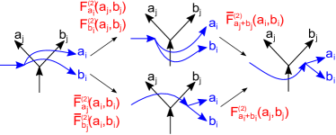
Figure 8: Self-consistency in sequences requires the condition (69).

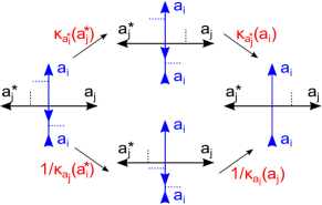
Figure 9: Self-consistency in sequences requires the condition (70).

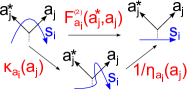
Figure 10: Self-consistency in sequences requires the condition (71).

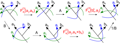
Figure 11: Self-consistency in sequences requires the condition (72). Here $A=\frac{\eta_{a_{i}}\left(a_{k}+b_{k}\right)}{\eta_{a_{i}}\left(b_{k}\right)\bar{F}_{a_{i}}^{\left(2\right)}\left(a_{k},b_{k}\right)}$ and $B=\bar{F}_{a_{j}}^{\left(2\right)}\left(a_{k},b_{k}\right).$

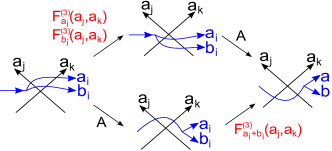
Figure 12: Self-consistency in sequences requires the condition (73). Here $A=\bar{F}^{(2)}_{a_{j}}(a_{i},b_{i})\bar{F}^{(2)}_{a_{k}}(a_{i},b_{i}).$

We have shown that Eqs. (67–76) are necessary conditions for the rules to be self-consistent. To show that they are sufficient, one can follow the same argument in Ref. Lin and Levin, 2014. Suppose that $\{F^{(2)},\kappa,\eta,F^{(3)}\}$ satisfy Eqs. (67–76) and use them to construct an exactly soluble lattice Hamiltonian $H$ $\left(\ref{ham}\right).$ Then the ground state of $H$ satisfies the local rules $\left(\ref{rule2a}\text{--\ref{rule2d}}\right)$ on the lattice. By using this fact, we can prove that the rules are self-consistent. Suppose, on the contrary, that the rules $\left(\ref{rule2a}\text{--\ref{rule2d}}\right)$ are not self-consistent. Then there exists two sequences of moves which relate the same initial and final continuum string-net states $X_{1},X_{2}$ but with different proportionality constants. These two sequences of moves can be adapted from the continuum to the lattice if we make the lattice sufficiently fine. However, this leads to a contradiction since the ground state wave function $\Phi_{latt}$ of $H$ obeys the rules on the lattice (see section V.2). Thus, our assumption is false. We conclude that the rules must be self-consistent.

Appendix B Graphical representation of the Hamiltonian

In this section, we demonstrate the graphical representation of $B_{p}^{s_{i}}$ leads to the matrix elements in equation (23).

By the graphical representation, the action of the operator $B_{p}^{s_{i}}$ on a string-net state is to add a loop of type-$s_{i}$ string. We can fuse the string $s_{i}$ onto the links along the boundary of the plaquette by using the local rules (1–3,7–11). This allows us to obtain the matrix elements of $B_{p}^{s_{i}}.$ Specifically, there are two steps in this fusion process. The first step is to glide the string $s_{i}$ over all other string-nets with different flavors inside the plaquette $p$. This gives the factors $B_{p,x^{\prime}x}^{s_{i}\left(2\right)}$ and $B_{p,x^{\prime}x}^{s_{i}\left(3\right)}$. Then, the second step is to fuse $s_{i}$ to the boundary links of $p$ as in the original construction which gives the factor $B_{p,x^{\prime}x}^{s_{i}\left(1\right)}$. The computation of $B_{p,x^{\prime}x}^{s_{i}(1)}$ is exactly the same as in the Appendix D of Ref. Lin and Levin, 2014 by neglecting string-nets of all other different flavors and thus we will not repeat here. We will present the graphical representation of computing $B_{p,x^{\prime}x}^{s_{i}(2)}$ and $B_{p,x^{\prime}x}^{s_{i}(3)}$.

Let us start with computing $B_{p,x^{\prime}x}^{s_{i}(2)}$. Since we focus on the phase factors from gliding the string $s_{i}$, we represent the honeycomb lattices by square lattices with proper splitting at vertices in mind (see Fig. 2). It is sufficient to consider gliding the string $s_{i}$ over the $j$-favor of string-nets, namely the 2-intersection between the $i$- and $j$-flavor of string-nets. Let $B_{ij}^{\left(2\right)}$ be the phase associated with gliding $s_{i}$ to the boundary of $p$. We first compute

$$\left\langle\raisebox{-16.62178pt}{\includegraphics[height=50.58878pt]{b20.eps}}\right|B_{p}^{s_{i}} =\left\langle\raisebox{-16.62178pt}{\includegraphics[height=50.58878pt]{b2a.eps}}\right|=\eta_{s_{i},g_{j}}\eta_{s_{i},b_{j}}\eta_{s_{i},c_{j}}F_{s_{i},g_{j}b_{j}}^{\left(2\right)}F_{s_{i},\left(g_{j}+b_{j}\right)c_{j}}^{\left(2\right)}\left\langle\raisebox{-16.62178pt}{\includegraphics[height=50.58878pt]{b2b.eps}}\right|$$

$$\sim\eta_{s_{i},g_{j}}\eta_{s_{i},b_{j}}\eta_{s_{i},c_{j}}F_{s_{i},g_{j}b_{j}}^{\left(2\right)}F_{s_{i},\left(g_{j}+b_{j}\right)c_{j}}^{\left(2\right)}\left\langle\raisebox{-16.62178pt}{\includegraphics[height=50.58878pt]{b2c.eps}}\right|$$

$$\sim\eta_{s_{i},g_{j}}\eta_{s_{i},b_{j}}\eta_{s_{i},c_{j}}F_{s_{i},g_{j}b_{j}}^{\left(2\right)}F_{s_{i},\left(g_{j}+b_{j}\right)c_{j}}^{\left(2\right)}F_{g_{j},s_{i}l_{i}}^{\left(2\right)}F_{b_{j},s_{i}g_{i}}^{\left(2\right)}F_{c_{j},s_{i}i_{i}}^{\left(2\right)}\tilde{F}_{i_{j},s_{i}j_{i}}^{\left(2\right)}\left\langle\raisebox{-16.62178pt}{\includegraphics[height=50.58878pt]{b2d.eps}}\right|\sim B_{ij}^{\left(2\right)}\left\langle\raisebox{-16.62178pt}{\includegraphics[height=50.58878pt]{b2e.eps}}\right|$$

with

$$B_{ij}^{\left(2\right)}=\eta_{s_{i},g_{j}}\eta_{s_{i},b_{j}}\eta_{s_{i},c_{j}}F_{s_{i},g_{j}b_{j}}^{\left(2\right)}F_{s_{i},\left(g_{j}+b_{j}\right)c_{j}}^{\left(2\right)}F_{g_{j},s_{i}l_{i}}^{\left(2\right)}F_{b_{j},s_{i}g_{i}}^{\left(2\right)}F_{c_{j},s_{i}i_{i}}^{\left(2\right)}\tilde{F}_{i_{j},s_{i}j_{i}}^{\left(2\right)}=\eta_{s_{i},i_{j}}\frac{F^{(2)}_{g_{j},s_{i}l_{i}}F^{(2)}_{b_{j},s_{i}g_{i}}F^{(2)}_{c_{j},s_{i}i_{i}}\bar{F}^{(2)}_{i_{j},s_{i}j_{i}}}{\bar{F}^{(2)}_{s_{i},g_{j}b_{j}}\bar{F}^{(2)}_{s_{i},(g_{j}+b_{j})c_{j}}}.$$

Here the symbol $\sim$ means equality up to phases in $B_{p,x^{\prime}x}^{s_{i}(1)}$ associated with fusing $s_{i}$ to the boundary links of $p$ and $x_{i}^{\prime}=x_{i}+s_{i}$ in the last two states. The last equality follows from the identity (94). The $B_{p,x^{\prime}x}^{s_{i}(2)}$ is then obtained by taking into account all types of 2-intersections inside the plaquette $p$, namely, $B_{p,x^{\prime}x}^{s_{i}(2)}=\prod_{j\neq i}B_{ij}^{\left(2\right)}$ as in Eq. (25).

Similarly, to obtain $B_{p,x^{\prime}x}^{s_{i}(3)}$, it suffices to consider gliding the string $s_{i}$ over the $j$- and $k$-flavor of string-nets, namely the 3-intersection among these three flavors of string-nets. Let $B_{ijk}^{\left(3\right)}$ be the phase factor associated with gliding $s_{i}$ over the intersections between $j$- and $k$-flavors of string-nets:

$$\left\langle\raisebox{-20.95781pt}{\includegraphics[height=50.58878pt]{b30.eps}}\right|B_{p}^{s_{i}}=\left\langle\raisebox{-20.95781pt}{\includegraphics[height=50.58878pt]{b3a.eps}}\right|\sim\left\langle\raisebox{-20.95781pt}{\includegraphics[height=50.58878pt]{b3b.eps}}\right|$$

$$\sim B_{ijk}^{(3)}\left\langle\raisebox{-20.95781pt}{\includegraphics[height=50.58878pt]{b3c.eps}}\right|\sim B_{ijk}^{(3)}\left\langle\raisebox{-20.95781pt}{\includegraphics[height=50.58878pt]{b3d.eps}}\right|$$

with

$$B_{ijk}^{(3)}=F^{(3)}_{s_{i}}(c_{k}^{*},i_{j})F^{(3)-1}_{s_{i}^{*}}(g_{j},b_{k}).$$ (77)

Here the symbol $\sim$ indicates equality up to phases in $B_{p,x^{\prime}x}^{s_{i}(2)}$ and $B_{p,x^{\prime}x}^{s_{i}(1)}$ associated with gliding $s_{i}$ over 2-intersections in $p$ and fusing $s_{i}$ to the boundary links of $p$. Therefore, $B_{p,x^{\prime}x}^{s_{i}(3)}$ is obtained by taking into account all kinds of 3-intersections inside $p$, namely, $B_{p,x^{\prime}x}^{s_{i}(3)}=\prod_{j\neq k\neq i}B_{ijk}^{\left(3\right)}$ as in Eq. (26). This completes our derivation of the Hamiltonian.

Appendix C Showing $B_{p_{1}}^{s_{i}}$ and $B_{p_{2}}^{s_{j}}$ commute

In this section, we will show that the operators $B_{p_{1}}^{s_{i}}$ and $B_{p_{2}}^{s_{j}}$ commute with one another. We only have to consider three cases. The first two cases are when $i,j$ are of the same flavor and $p_{1}=p_{2}=p$ or $p_{1},p_{2}$ are adjacent. The third case is when $i,j$ are of different flavors and $p_{1}=p_{2}=p$. In last case, the two plaquettes at $p$ on different lattices are overlapped as shown in Fig. 13. When $p_{1},p_{2}$ are further apart, the two operators will commute.

The first case is when $i=j$ and $p_{1}=p_{2}=p$. To prove $[B_{p}^{s_{i}},B_{p}^{t_{i}}]=0$, it is sufficient to show that

$$B_{p,x^{\prime}y}^{s_{i}(m)}B_{p,yx}^{t_{i}(m)}=B_{p,x^{\prime}z}^{t_{i}(m)}B_{p,zx}^{s_{i}(m)}$$ (78)

holds for each component $m=1,2,3$. Here $x,x^{\prime}$ denote a set of spin labels for initial and final state configurations and $y,z$ denote a set of spin labels for the intermediate state configurations after acting $B_{p}^{t_{i}}$ and $B_{p}^{s_{i}}$ to the initial state, respectively. For the $m=1$ component, the proof is identical to the one given in Ref. Lin and Levin, 2014. They showed that

$$B_{p,x^{\prime}y}^{s_{i}(1)}B_{p,yx}^{t_{i}(1)}=B_{p,x^{\prime}z}^{t_{i}(1)}B_{p,zx}^{s_{i}(1)}=B_{p,x^{\prime}x}^{s_{i}+t_{i}(1)}$$ (79)

Similarly, for the $m=2$ component, one can show that

$$B_{p,x^{\prime}y}^{s_{i}(2)}B_{p,yx}^{t_{i}(2)}=B_{p,x^{\prime}z}^{t_{i}(2)}B_{p,zx}^{s_{i}(2)}=B_{p,x^{\prime}x}^{s_{i}+t_{i}(2)}.$$ (80)

To see this, one can write down the expression of $B_{p,x^{\prime}y}^{s_{i}(2)}B_{p,yx}^{t_{i}(2)}$:

$$B_{p,x^{\prime}y}^{s_{i}(2)}B_{p,yx}^{t_{i}(2)}= \eta_{t_{i},i_{j}}\frac{F^{(2)}_{g_{j},t_{i}l_{i}}F^{(2)}_{b_{j},t_{i}g_{i}}F^{(2)}_{c_{j},t_{i}i_{i}}\bar{F}^{(2)}_{i_{j},t_{i}j_{i}}}{\bar{F}^{(2)}_{t_{i},g_{j}b_{j}}\bar{F}^{(2)}_{t_{i},(g_{j}+b_{j})c_{j}}}\times$$

$$\eta_{s_{i},i_{j}}\frac{F^{(2)}_{g_{j},t_{i}l_{i}^{\prime}}F^{(2)}_{b_{j},t_{i}g_{i}^{\prime}}F^{(2)}_{c_{j},t_{i}i_{i}^{\prime}}\bar{F}^{(2)}_{i_{j},t_{i}j_{i}^{\prime}}}{\bar{F}^{(2)}_{s_{i},g_{j}b_{j}}\bar{F}^{(2)}_{s_{i},(g_{j}+b_{j})c_{j}}}$$

where $a_{i}^{\prime}=a_{i}+t_{i}$ with $a_{i}\in\{l_{i},g_{i},i_{i},j_{i}\}$. By using (19a) $F^{(2)}_{a_{j},t_{i}a_{i}}F^{(2)}_{a_{j},s_{i}a_{i}^{\prime}}=F^{(2)}_{a_{j},(s_{i}+t_{i})a_{i}}F^{(2)}_{a_{j},s_{i}t_{i}}$ and (19b) $\bar{F}^{(2)}_{t_{i},a_{j}b_{j}}\bar{F}^{(2)}_{s_{i},a_{j}b_{j}}=\bar{F}^{(2)}_{(s_{i}+t_{i}),a_{j}b_{j}}F^{(2)}_{a_{j},s_{i}t_{i}}F^{(2)}_{b_{j},s_{i}t_{i}}/F^{(2)}_{(a_{j}+b_{j}),s_{i}t_{i}}$ and (94) $\bar{F}^{(2)}_{a_{j},s_{i}t_{i}}F^{(2)}_{a_{j},s_{i}t_{i}}=\eta_{i_{j},{s_{i}+t_{i}}}/\eta_{i_{j},s_{i}}\eta_{i_{j},t_{i}}$, the above expression can be rewritten as

$$B_{p,x^{\prime}y}^{s_{i}(2)}B_{p,yx}^{t_{i}(2)} =\eta_{u_{i},i_{j}}\frac{F^{(2)}_{g_{j},u_{i}l_{i}}F^{(2)}_{b_{j},u_{i}g_{i}}F^{(2)}_{c_{j},u_{i}i_{i}}\bar{F}^{(2)}_{i_{j},u_{i}j_{i}}}{\bar{F}^{(2)}_{u_{i},g_{j}b_{j}}\bar{F}^{(2)}_{u_{i},(g_{j}+b_{j})c_{j}}}=B_{p,x^{\prime}x}^{u_{i}(2)}$$

with $u_{i}=s_{i}+t_{i}$. This shows (80).

Finally, it is easy to see from (26) and (19g) that (78) also holds for $m=3$. Thus, putting everything together, we conclude that

$$B_{p}^{s_{i}}B_{p}^{t_{i}}=B_{p}^{t_{i}}B_{p}^{s_{i}}=B_{p}^{s_{i}+t_{i}}$$ (81)

showing the commutativity when $i=j$ and $p_{1}=p_{2}=p$.

The second case is when $i=j$ and $p_{1},p_{2}$ are adjacent plaquettes. We want to show $[B_{p_{1}}^{s_{i}},B_{p_{2}}^{t_{i}}]=0$. To prove this, it is sufficient to show that

$$B_{p_{1},x^{\prime}y}^{s_{i}(m)}B_{p_{2},yx}^{t_{i}(m)}=B_{p_{2},x^{\prime}z}^{t_{i}(m)}B_{p_{1},zx}^{s_{i}(m)}$$ (82)

holds for $m=1,2,3$. The proof for $m=1$ is identical to the one in the appendix E of Ref. Lin and Levin, 2014. It is also easy to see that (82) holds for $m=2,3$ since the intersections between different flavors of strings are away from the link shared by two plaquettes $p_{1},p_{2}$. This establishes $[B_{p_{1}}^{s_{i}},B_{p_{2}}^{t_{i}}]=0$.

Finally, we consider the case where $i\neq j$ and $p_{1}=p_{2}=p$. We want to show $[B_{p}^{s_{i}},B_{p}^{s_{j}}]=0$ with $B_{p}^{s_{i}},B_{p}^{s_{j}}$ acting on two overlapping plaquettes shown in Fig. 13. To prove $[B_{p}^{s_{i}},B_{p}^{s_{j}}]=0$, it is sufficient to show that

$$B_{p,x^{\prime}y}^{s_{i}(m)}B_{p,yx}^{s_{j}(m)}=B_{p,x^{\prime}z}^{s_{j}(m)}B_{p,zx}^{s_{i}(m)}$$ (83)

for $m=1,2,3$. Again, $x,x^{\prime}$ denote a set of spin labels for the initial and final state configurations while $y,z$ denote a set of spin labels for the intermediate state configurations after acting $B_{p}^{s_{j}}$ and $B_{p}^{s_{i}}$ to the initial state. In this case, it is easy to see that (83) holds for $m=1,3$ by writing down the phase factors on each side using (24,26). Thus all that remains is to show that (83) holds for $m=2$.

We can write down each side of (83) for $m=2$ by (25):

$$LHS =\bar{F}_{i_{j},s_{i}j_{i}}^{\left(2\right)}F_{g_{j},s_{i}l_{i}}^{\left(2\right)}F_{s_{i},g_{j}b_{j}}^{\left(2\right)}F_{s_{i},\left(g_{j}+b_{j}\right)c_{j}}^{\left(2\right)}\eta_{s_{i},g_{j}}\times$$

$$F_{j_{i}^{\prime},s_{j}i_{j}}^{\left(2\right)}\bar{F}_{l_{i}^{\prime},s_{j}g_{j}}^{\left(2\right)}F_{s_{j},j_{i}^{\prime}e_{i}}^{\left(2\right)}F_{s_{j},\left(j_{i}^{\prime}+e_{i}\right)f_{i}}^{\left(2\right)}\eta_{s_{j},j_{i}^{\prime}}$$ (84)

$$RHS =F_{j_{i},s_{j}i_{j}}^{\left(2\right)}\bar{F}_{l_{i},s_{j}g_{j}}^{\left(2\right)}F_{s_{j},j_{i}e_{i}}^{\left(2\right)}F_{s_{j},\left(j_{i}+e_{i}\right)f_{i}}^{\left(2\right)}\eta_{s_{j},j_{i}}\times$$

$$\bar{F}_{i_{j}^{\prime},s_{i}j_{i}}^{\left(2\right)}F_{g_{j}^{\prime},s_{i}l_{i}}^{\left(2\right)}F_{s_{i},g_{j}^{\prime}b_{j}}^{\left(2\right)}F_{s_{i},\left(g_{j}^{\prime}+b_{j}\right)c_{j}}^{\left(2\right)}\eta_{s_{i},g_{j}^{\prime}}.$$ (85)

where $a_{i}^{\prime}=a_{i}+s_{i}$ with $a_{i}\in\{j_{i},l_{i}\}$ and $a_{j}^{\prime}=a_{j}+s_{j}$ with $a_{j}\in\{i_{j},g_{j}\}$. Here we only keep the relevant factors which involve $i_{j},g_{j},l_{i},j_{i}$ strings. To show $\left(\ref{e1}\right)=\left(\ref{e2}\right),$ we first use $\left(\ref{3f}\right)$ to simplify both sides so that all phase factors have subindices $s_{i}$ or $s_{j}.$ Then to show the equality is equivalent to show $C_{L}=C_{R}$ with

$$C_{L}=\frac{F_{s_{i},g_{j}b_{j}}^{\left(2\right)}F_{s_{i},\left(g_{j}+b_{j}\right)c_{j}}^{\left(2\right)}F_{s_{i},s_{j}i_{j}}^{\left(2\right)}\bar{F}_{s_{i},s_{j}g_{j}}^{\left(2\right)}\eta_{s_{i},g_{j}}}{F_{s_{i},g_{j}^{\prime}b_{j}}^{\left(2\right)}F_{s_{i},\left(g_{j}^{\prime}+b_{j}\right)c_{j}}^{\left(2\right)}\eta_{s_{i},g_{j}^{\prime}}}$$

and

$$C_{R}=\frac{F_{s_{j},j_{i}e_{i}}^{\left(2\right)}F_{s_{j},\left(j_{i}+e_{i}\right)f_{i}}^{\left(2\right)}F_{s_{j},s_{i}l_{i}}^{\left(2\right)}\bar{F}_{s_{j,}s_{i}j_{i}}^{\left(2\right)}\eta_{s_{j},j_{i}}}{F_{s_{j},j_{i}^{\prime}e_{i}}^{\left(2\right)}F_{s_{j},\left(j_{i}^{\prime}+e_{i}\right)f_{i}}^{\left(2\right)}\eta_{s_{j},j_{i}^{\prime}}}.$$

To proceed, we use $\left(\ref{sfeq1}\right)$ and the facts $j_{i}+e_{i}+f_{i}=l_{i}$ and $g_{j}+b_{j}+c_{j}=i_{j}$ to obtain

$$C_{L} =F_{s_{i},s_{j}g_{j}}^{\left(2\right)}\bar{F}_{s_{i},s_{j}g_{j}}^{\left(2\right)}\frac{\eta_{s_{i},g_{j}}}{\eta_{s_{i},g_{j}^{\prime}}},$$

$$C_{R} =F_{s_{j},s_{i}j_{i}}^{\left(2\right)}\bar{F}_{s_{j},s_{i}j_{i}}^{\left(2\right)}\frac{\eta_{s_{j},j_{i}}}{\eta_{s_{j},j_{i}^{\prime}}}.$$

Furthermore, we use (94) to rewrite

$$C_{L}=\frac{1}{\eta_{s_{i},s_{j}}},\quad C_{R}=\frac{1}{\eta_{s_{j},s_{i}}}.$$ (86)

Finally, by (19h), we show $C_{L}=C_{R}$. This completes the proof that $B_{p}^{s_{i}},B_{p}^{s_{j}}$ commute with one another.

Figure 13: Two plaquette operators $B_{p}^{s_{i}}$ and $B_{p}^{s_{j}}$ act on two overlapped (red and blue shaded) plaquettes.

Appendix D Properties of the Hamiltonian (22)

In this section, we establish the following properties of the Hamiltonian (22):

1. $(B_{p}^{s_{i}})^{\dagger}=B_{p}^{s_{i}}$.

2. $B_{p}^{i}$ is a projection operator, namely, $B_{p}^{i2}=B_{p}^{i}$.

3. The ground state wave function on the honeycomb lattice satisfies the local rules (1–2,7–11).

Let us show them in order. To show the first equality, we need to show the matrix elements on both sides are equal, namely $(B_{p,xx^{\prime}}^{s_{i}})^{*}=B_{p,x^{\prime}x}^{s^{*}_{i}}$ with $x,x^{\prime}$ being the spin labels for the initial and final states after the action of $B_{p}^{s_{i}}$ on the initial state. By (20), we can rewrite the equality as $B_{p,xx^{\prime}}^{s^{*}_{i}-1}=B_{p,x^{\prime}x}^{s_{i}}$. Since $B_{p,xx^{\prime}}^{s_{i}}$ can be written as a product of three components $B_{p,xx^{\prime}}^{s_{i}(1)}B_{p,xx^{\prime}}^{s_{i}(2)}B_{p,xx^{\prime}}^{s_{i}(3)}$ (see Eq. (23), thus it is sufficient to show the equality to hold for each component.

Ref. Lin and Levin, 2014 showed that $B_{p,xx^{\prime}}^{s_{i}^{*}(1)-1}=B_{p,x^{\prime}x}^{s_{i}(1)}$ (see Appendix F therein). It is also easy to see $B_{p,xx^{\prime}}^{s_{i}^{*}(3)-1}=B_{p,x^{\prime}x}^{s_{i}(3)}$ by using $F^{(3)}_{a_{i},a_{j}a_{k}}=F^{(3)-1}_{a^{*}_{i},a_{j}a_{k}}$ (Eq. (19g) with $b_{i}=a_{i}^{*}$) to simplify $B_{p,xx^{\prime}}^{s_{i}^{*}(3)-1}$. All that remains is to show that $B_{p,xx^{\prime}}^{s_{i}^{*}(2)-1}=B_{p,x^{\prime}x}^{s_{i}(2)}$. To this end, we write down $B_{p,xx^{\prime}}^{s_{i}^{*}(2)-1}$ explicitly

$$B_{p,xx^{\prime}}^{s_{i}^{*}(2)-1}=\eta_{s^{*}_{i},i_{j}}\frac{F^{(2)}_{g_{j},s_{i}^{*}l_{i}^{\prime}}F^{(2)}_{b_{j},s_{i}^{*}g_{i}^{\prime}}F^{(2)}_{c_{j},s_{i}^{*}i_{i}^{\prime}}\bar{F}^{(2)}_{i_{j},s_{i}^{*}j_{i}^{\prime}}}{\bar{F}^{(2)}_{s_{i}^{*},g_{j}b_{j}}\bar{F}^{(2)}_{s_{i}^{*},(g_{j}+b_{j})c_{j}}}$$ (87)

where $a_{i}^{\prime}=a_{i}+s_{i}$ with $a_{i}\in\{g_{i},l_{i},j_{i}\}$. To proceed, we use the identity $F^{(2)}_{a_{j},s_{i}^{*}a_{i}^{\prime}}=F^{(2)}_{a_{j},s_{i}^{*}s_{i}}/F^{(2)}_{a_{j},s_{i}a_{i}}$ (which can be obtained from (19a)) and a similar identity for $\bar{F}^{(2)}$ to reexpress $F^{(2)},\bar{F}^{(2)}$ in the numerator of (87) while we use (19b) to rewrite $\bar{F}^{(2)}$ in the denominator. Next, we use (19e,93) to express $F^{(2)}_{a_{j},s_{i}^{*}s_{i}},\bar{F}^{(2)}_{a_{j},s_{i}^{*}s_{i}}$ in terms of $\eta,\kappa$. Finally, we use (92) and (94) to simplify the expression to $B_{p,x^{\prime}x}^{s_{i}(2)}$. This establishes the first property.

To prove the second result, we use the identity (81) to derive

$$B_{p}^{i2}=\sum_{s_{i},t_{i}}\frac{d_{s_{i}}d_{t_{i}}}{|G|^{2}}B_{p}^{s_{i}}B_{p}^{t_{i}}=\sum_{s_{i},t_{i}}\frac{d_{s_{i}}d_{t_{i}}}{|G|^{2}}B_{p}^{s_{i}+t_{i}}.$$ (88)

We then use (6) to write $d_{s_{i}}d_{t_{i}}=d_{s_{i}+t_{i}}$. After changing variables to $u_{i}=s_{i}+t_{i}$, we derive

$$B_{p}^{i2}=\sum_{u_{i}}\frac{d_{u_{i}}}{|G|}B_{p}^{u_{i}}=B_{p}^{i}.$$ (89)

Finally, we show that the ground state $\Phi_{latt}$ of $H$ obeys the local rules (1–3) and (7–11). The proof that $\Phi_{latt}$ obeys (1–3) is identical to the one in appendix F of Ref. Lin and Levin, 2014. Here we only show that $\Phi_{latt}$ obeys (7–11). To see this, we use the fact that $B_{p}^{i}|\Psi_{latt}\rangle=|\Phi_{latt}\rangle$ together with the following relations:

$$\left\langle\raisebox{-18.06749pt}{\includegraphics[height=46.97505pt]{state1a.eps}}\right|B_{p}^{i} =F^{(2)}_{a_{i}}(a_{j},b_{j})\left\langle\raisebox{-18.06749pt}{\includegraphics[height=46.97505pt]{state1b.eps}}\right|B_{p}^{i},$$ (90)

$$\left\langle\raisebox{-18.06749pt}{\includegraphics[height=46.97505pt]{state2a.eps}}\right|B_{p}^{i} =\bar{F}^{(2)}_{a_{i}}(a_{j},b_{j})\left\langle\raisebox{-18.06749pt}{\includegraphics[height=46.97505pt]{state2b.eps}}\right|B_{p}^{i},$$

$$\left\langle\raisebox{-18.06749pt}{\includegraphics[height=46.97505pt]{state3a.eps}}\right|B_{p}^{i} =\kappa_{a_{i}}(a_{j})\left\langle\raisebox{-18.06749pt}{\includegraphics[height=46.97505pt]{state3b.eps}}\right|B_{p}^{i},$$

$$\left\langle\raisebox{-18.06749pt}{\includegraphics[height=46.97505pt]{state4a.eps}}\right|B_{p}^{i} =\eta_{a_{i}}(a_{j})\left\langle\raisebox{-18.06749pt}{\includegraphics[height=46.97505pt]{state4b.eps}}\right|B_{p}^{i},$$

$$\left\langle\raisebox{-18.06749pt}{\includegraphics[height=46.97505pt]{state5a.eps}}\right|B_{p}^{i} =F^{(3)}_{a_{i}}(a_{j},a_{k})\left\langle\raisebox{-18.06749pt}{\includegraphics[height=46.97505pt]{state5b.eps}}\right|B_{p}^{i}.$$

Multiplying the above equations by the ground state $|\Phi_{latt}\rangle$, one can immediately see that the ground state wave function $\Phi_{latt}(X)=\langle X|\Phi_{latt}\rangle$ satisfies the local rules (7–11).

The relations (90) can be shown by using the expression for the matrix elements of $B_{p}^{s_{i}}$ in (23) together with (19a–19j). Here we prove the first equation for example. First, we expand the left hand side as

$$\left\langle\raisebox{-18.06749pt}{\includegraphics[height=46.97505pt]{state1a.eps}}\right|B_{p}^{i}=\sum_{s_{i}}\frac{d_{s_{i}}}{|G|}\left\langle\raisebox{-18.06749pt}{\includegraphics[height=46.97505pt]{state1a1.eps}}\right|$$

$$=\sum_{s_{i}}\frac{d_{s_{i}}}{|G|}B^{(1),a_{i}^{*}a_{i}^{*}a_{i}^{*}000}_{a_{i}^{*\prime}a_{i}^{*\prime}a_{i}^{*\prime}s_{i}s_{i}s_{i}}(a_{i}^{*}00a_{i}00)\times$$

$$\eta_{s_{i},a_{j}+b_{j}}\frac{F^{(2)_{a_{j},s_{i}a_{i}*}}F^{(2)}_{b_{j},s_{i}a_{i}^{*}}}{\bar{F}^{(2)}_{s_{i},a_{j}b_{j}}}\kappa_{a_{j},a_{i}}\kappa_{b_{j},a_{i}}\left\langle\raisebox{-18.06749pt}{\includegraphics[height=46.97505pt]{state1a2.eps}}\right|.$$

Here $B_{p}^{(1)}$ is defined in (24) and $a^{\prime}_{i}=a_{i}+s_{i}$. Similarly, the right hand side is given by

$$\left\langle\raisebox{-18.06749pt}{\includegraphics[height=46.97505pt]{state1b.eps}}\right|B_{p}^{i}=\sum_{s_{i}}\frac{d_{s_{i}}}{|G|}\left\langle\raisebox{-18.06749pt}{\includegraphics[height=46.97505pt]{state1b1.eps}}\right|$$

$$=\sum_{s_{i}}\frac{d_{s_{i}}}{|G|}B^{(1),000a_{i}a_{i}a_{i}}_{s_{i}s_{i}s_{i}a_{i}^{\prime}a_{i}^{\prime}a_{i}^{\prime}}(a_{i}^{*}00a_{i}00)\times$$

$$\eta_{s_{i},a_{j}+b_{j}}\frac{\bar{F}^{(2)_{a_{j}+b_{j},s_{i}a_{i}}}}{\bar{F}^{(2)}_{s_{i},a_{j}b_{j}}}\left\langle\raisebox{-18.06749pt}{\includegraphics[height=46.97505pt]{state1b2.eps}}\right|.$$

By changing the dummy variables $s_{i}$ to $s_{i}+a_{i}$ in the first expression, we can see the final states for the two expressions are the same. We then compute the ratio of the two corresponding amplitudes. By using (19a–19c), this ratio can be simplified to $F^{(2)}_{a_{i}}(a_{j},b_{j})$. This justifies the first equation in (90). The other equations can be shown in the same manner.

Appendix E Some useful identities

In this section, we collect some useful identities which are used in previous appendices.

First, let $b_{j}=a_{j}^{\ast}=c_{j}^{\ast}$ in (19a) and get

$$F_{a_{i}}^{\left(2\right)}\left(a_{j},a_{j}^{\ast}\right)=F_{a_{i}}^{\left(2\right)}\left(a_{j}^{\ast},a_{j}\right).$$ (91)

Second, from (19e) and (91), we get

$$\frac{\eta_{x}\left(a^{\ast}\right)}{\eta_{x}\left(a\right)}=\frac{\kappa_{x}\left(a^{\ast}\right)}{\kappa_{x}\left(a\right)}.$$ (92)

Third, let $b_{j}=a_{j}^{*}$ in (19b), use (19e) to express $F^{(2)}$ in terms of $\eta,\kappa$ and finally use (19d) to simplify the expression. We get the analog of (19e) for $\bar{F}^{(2)}$:

$$\kappa_{a_{i}}^{-1}\left(a_{j}^{\ast}\right) =\bar{F}_{a_{i}}^{\left(2\right)}\left(a_{j}^{\ast},a_{j}\right)\eta_{a_{i}}\left(a_{j}\right).$$ (93)

Finally, let $b_{i}=a_{i}^{*}$ in (19c) and use (93) to express $\bar{F}^{(2)}$ in terms of $\eta,\kappa$ and finally use (19d) to simplify the expression. We get an alternative expression for $\bar{F}^{(2)}$ (c.f. Eq. (19b)):

$$\bar{F}_{a_{i}}^{\left(2\right)}\left(a_{j},b_{j}\right)=F_{a_{i}}^{\left(2\right)-1}\left(a_{j},b_{j}\right)\frac{\eta_{a_{i}}\left(a_{j}+b_{j}\right)}{\eta_{a_{i}}\left(a_{j}\right)\eta_{a_{i}}\left(b_{j}\right)}.$$ (94)

References

- Wen (2007) Xiao-Gang Wen, Quantum Field Theory of Many-body Systems: From the Origin of Sound to an Origin of Light and Electrons (Oxford University Press, 2007).
- Kitaev (2003) Alexei Yu Kitaev, “Fault-tolerant quantum computation by anyons,” Annals of Physics 303, 2–30 (2003).
- Levin and Wen (2005) Michael A. Levin and Xiao-Gang Wen, “String-net condensation: A physical mechanism for topological phases,” Phys. Rev. B 71, 045110 (2005).
- Lan and Wen (2014) Tian Lan and Xiao-Gang Wen, “Topological quasiparticles and the holographic bulk-edge relation in -dimensional string-net models,” Phys. Rev. B 90, 115119 (2014).
- Hu et al. (2013) Yuting Hu, Yidun Wan, and Yong-Shi Wu, “Twisted quantum double model of topological phases in two–dimension,” Phys. Rev. B 87, 125114 (2013).
- Mesaros and Ran (2013) Andrej Mesaros and Ying Ran, “A classification of symmetry enriched topological phases with exactly solvable models,” Phys. Rev. B 87, 155115 (2013).
- Kitaev and Kong (2012) Alexei Kitaev and Liang Kong, “Models for gapped boundaries and domain walls,” Commun. Math. Phys. 313, 351 (2012).
- Kong (2014) Liang Kong, “Some universal properties of levin-wen models,” in Proceedings of XVIITH International Congress of Mathematical Physics (2014) p. 444.
- Lin and Levin (2014) Chien-Hung Lin and Michael Levin, “Generalizations and limitations of string-net models,” Phys. Rev. B 89, 195130 (2014).
- Kitaev (2006) Alexei Kitaev, “Anyons in an exactly solved model and beyond,” Ann. Phys. 321, 2 (2006).
- Bonderson (2007) Parsa Hassan Bonderson, Non-abelian anyons and interferometry, Ph.D. thesis, California Institute of Technology (2007).
- Chen et al. (2013) Xie Chen, Zheng-Cheng Gu, Zheng-Xin Liu, and Xiao-Gang Wen, “Symmetry-protected topological orders and the cohomology class of their symmetry group,” Phys. Rev. B 87, 155114 (2013).
- Jagannathan (1985) R. Jagannathan, “On projective representations of finite abelian groups,” in Number Theory: Proceedings of the 4th Matscience Conference held at Ootacamund, India, January 5–10, 1984, edited by Krishnaswami Alladi (Springer Berlin Heidelberg, Berlin, Heidelberg, 1985) pp. 130–139.
- Propitius (1995) Mark de Wild Propitius, Topological interactions in broken gauge theories, Ph.D. thesis, University of Amsterdam (1995).
- Wang and Levin (2015) Chenjie Wang and Michael Levin, “Topological invariants for gauge theories and symmetry-protected topological phases,” Phys. Rev. B 91, 165119 (2015).
- Chen et al. (2014) Xie Chen, Yuan-Ming Lu, and Ashvin Vishwanath, “Symmetry-protected topological phases from decorated domain walls,” Nature Communications 5, 3507 (2014).
- Levin and Gu (2012) Michael Levin and Zheng-Cheng Gu, “Braiding statistics approach to symmetry-protected topological phases,” Phys. Rev. B 86, 115109 (2012).
- Gu et al. (2016) Zheng-Cheng Gu, Juven C. Wang, and Xiao-Gang Wen, “Multikink topological terms and charge-binding domain-wall condensation induced symmetry-protected topological states: Beyond chern-simons/bf field theories,” Phys. Rev. B 93, 115136 (2016).
- He et al. (2016) Huan He, Yunqin Zheng, and Curt von Keyserlingk, “Field theories for gauged symmetry protected topological phases: Abelian gauge theories with non-abelian quasiparticles,” arxiv:1105.4351 (2016).
- Heinrich et al. (2016) Chris Heinrich, Fiona Burnell, Lukasz Fidkowski, and Michael Levin, “Symmetry enriched string-nets: Exactly solvable models for set phases,” arXiv:1606.07816 (2016).
- Cheng et al. (2016) Meng Cheng, Zheng-Cheng Gu, Shenghan Jiang, and Yang Qi, “Exactly solvable models for symmetry-enriched topological phases,” arXiv:1606.08482 (2016).
- Barkeshli et al. (2014) Maissam Barkeshli, Parsa Bonderson, Meng Cheng, and Zhenghan Wang, “Symmetry, defects, and gauging of topological phases,” arxiv:1410.4540 (2014).