Zonostrophic instability driven by discrete particle noise

Abstract

The consequences of discrete particle noise for a system possessing a possibly unstable collective mode are discussed. It is argued that a zonostrophic instability (of homogeneous turbulence to the formation of zonal flows) occurs just below the threshold for linear instability. The scenario provides a new interpretation of the random forcing that is ubiquitously invoked in stochastic models such as the second-order cumulant expansion (CE2) or stochastic structural instability theory (SSST); neither intrinsic turbulence nor coupling to extrinsic turbulence is required. A representative calculation of the zonostrophic neutral curve is made for a simple two-field model of toroidal ion-temperature-gradient-driven modes. To the extent that the damping of zonal flows is controlled by the ion–ion collision rate, the point of zonostrophic instability is independent of that rate.

I Introduction

The zonostrophic instabilitySrinivasan and Young (2012) of a statistically homogeneous steady state to inhomogeneous zonal flows figures importantly in current research on the physics of zonal-flow generation and the interaction of zonal flows with turbulence. The general framework, called statistical state dynamics by Farrell and Ioannou,Farrell and Ioannou (2015) is intrinsically a statistical formalism — perturbations are made to a statistical ensemble, not a particular realization. Analytical treatment must therefore involve some sort of stochastic model. Considerable attention has been given to low-order cumulant truncations, in particular the CE2 (second-order cumulant expansion) studied by Tobias and MarstonTobias, Dagon, and Marston (2011); Tobias and Marston (2013); Marston, Qi, and Tobias (2016) and the closely related (in some cases mathematically identical) SSST or S3T (stochastic structural stability theory) introduced earlier by Farrell and Ioannou.Farrell and Ioannou (2003, 2009) A brief introduction to these topics is given in Sec. 6.3 of reference Krommes, 2015. In CE2 the so-called eddy–eddy nonlinearities are neglected; only the interactions between the turbulence and the zonal flows are retained. Generally the turbulence is driven by a white-noise stochastic forcing ${\widetilde{f}}$, for which various interpretations have been given. Sometimes, especially in S3T papers, it is taken to represent the effects of the missing eddy–eddy interactions. In strict CE2, it is instead taken to represent the effects of extrinsic fluctuations — e.g., baroclinic instabilities — whose dynamics are not described by the partial differential equation under study. In the present paper we introduce a variant of this latter interpretation; we attribute ${\widetilde{f}}$ to the discrete particle noise of a weakly coupled many-body plasma. We describe the relationship of this viewpoint to Kadomtsev’s classic discussion of the transition from stable to unstable collective modes, and we illustrate with a calculation of the neutral curve for the zonostrophic instability of a simple model of the toroidal ion-temperature-gradient (ITG) instability. New insights about the onset of the Dimits shift follow.

In Kadomtsev’s famous review/monograph,Kadomtsev (1965) he considered the following equation for fluctuation intensity $I$ (we have altered his notation slightly):

$$\frac{dI}{dt}=2\gamma I-2\alpha I^{2}+2F.$$ (1)

Here $\gamma$ is the linear growth rate of a collective mode, $\alpha$ is a positive mode-coupling coefficient, the $I^{2}$ term describes the possibility of nonlinear saturation of the linear instability, and $F$ describes the (small) level of noise due to discrete particles. (This equation and many other facets of Kadomtsev’s book are discussed in a lengthy tutorial article by Krommes.Krommes (2015)) In thermal equilibrium, $\gamma$ can be interpreted as the negative of the Landau-damping rate of a typical fluctuation with $k\lambda_{D}\ll 1$, where $\lambda_{D}$ is the Debye length [$\lambda_{D}^{-2}=\sum_{s}k_{{D}s}^{2}$, with $k_{{D}s}\doteq(4\pi n_{s}q_{s}^{2}/T)^{1/2}$ being the Debye wave number for species $s$]. Out of thermal equilibrium, it is assumed that $F$ remains unchanged while $\gamma$ changes as an order parameter (e.g., the temperature gradient $\kappa$) is varied. For stable plasma ($\gamma<0$), the steady-state balance is

$$I\approx F/|\gamma|.$$ (2)

As $\gamma\to 0_{-}$, that approximate level diverges. However, as the fluctuations become sufficiently large, the mode-coupling term takes over and permits a smooth transition through the point $\gamma=0$; for large $\gamma$, the nonlinear saturation level is $I\approx\gamma/\alpha$. Of course, the steady-state solution of the quadratic equation (1) can be found exactly; it is graphed in Fig. 1.

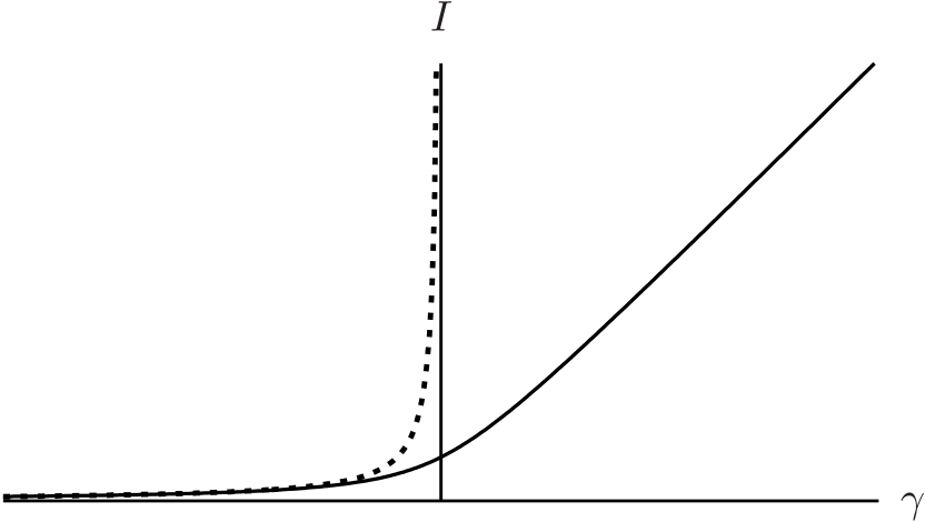
Figure 1: Solid curve: Steady-state solution of Eq. (1). Dashed curve: Approximate solution when the quadratic mode-coupling term is neglected.

The mode-coupling term $\propto I^{2}$ in Eq. (1) implicitly assumes turbulence; it represents the net effect of the statistical closureKrommes (2002, 2015) of a quadratic nonlinearity. Thus it does not capture the Dimits-shift phenomenon. The Dimits shift was first observed in the computer simulations described in LABEL:Dimits_shift. It refers to the fact that as the background temperature gradient $\kappa$ is varied from below to above the linear threshold $\kappa_{\rm c}$ for instability (the focus of Dimits et al. was on the ITG instability), the ion heat flux $Q(\kappa)$ turns on not for $\kappa>\kappa_{\rm c}$ but only for a larger value $\kappa>\kappa_{\mathchoice{*}{\displaystyle*}{\textstyle*}{\scriptstyle*}}>\kappa_{\rm c}$. The difference $\kappa_{\mathchoice{*}{\displaystyle*}{\textstyle*}{\scriptstyle*}}-\kappa_{\rm c}$ is called the Dimits shift. It is understood that the suppression of heat flux in the Dimits-shift regime is due to the excitation of zonal flows.Dimits et al. (2000); Rogers, Dorland, and Kotschenreuther (2000) In that regime, there is no turbulence, so conventional statistical closure does not apply. It is of interest to understand how the transition to turbulence is modified when the physics of the Dimits shift is included.

In the parlance of CE2 or S3T, the mode-coupling considered by Kadomtsev describes only the effect of the eddy–eddy interactions. Those stochastic models, which although quite simple have been surprisingly successful in various contexts, neglect the eddy–eddy interactions altogether, but do consider the interaction of zonal modes with turbulence. They are also tractable, so they provide a good starting point for further investigations. However, in the regimes of linear stability and the Dimits shift, there is no turbulence (we exclude the possibility of subcritical turbulence in this discussion), so the S3T interpretation of ${\widetilde{f}}$ as representing the effects of turbulent eddy–eddy interactions is not viable. Instead, we shall use CE2 and interpret ${\widetilde{f}}$ as being due to discrete particle noise, which is an extrinsic forcing from the point of view of the collective ITG dynamics. We assume that zonal modes are not driven directly by the particle noise (a very weak effect), but only by the Reynolds stress due to collective modes. The following scenario then pertains. In the absence of zonal flows, the balance (2) between particle noise and modal damping creates a statistically homogeneous steady state (in agreement with Kadomtsev’s interpretation). For sufficiently large Landau damping or sufficiently small $\kappa$, the homogeneous fluctuation level is small and the homogeneous state is stable against the formation of inhomogeneous zonal modes (which suffer a small but finite amount of collisional damping). Now imagine increasing $\kappa$, thereby driving the collective modes toward the threshold for linear instability. If zonal modes would never form, then the fluctuation intensity would diverge as $\gamma\to 0_{-}$, as does the dashed curve in Fig. 1. However, as $\gamma\to 0_{-}$ the forcing represented by the right-hand side of Eq. (2) becomes relatively large and, on the average, overcomes the damping on the zonal modes; a zonostrophic instabilitySrinivasan and Young (2012) (a supercritical bifurcation) occurs somewhere to the left of the linear threshold $\gamma=0$ ($\kappa=\kappa_{\rm c}$). These two thresholds are clearly distinct, with the zonostrophic one involving nonlinear effects. In the context of the ITG problem, the latter threshold defines the left-hand boundary of the Dimits-shift regime.Dimits et al. (2000) This interpretation of that boundary, as being related to a zonostrophic instability driven by discrete particle noise, is new.

To the extent that the particle noise is very small (as it is in hot, magnetically confined fusion plasmas), it might be thought that the zonostrophic threshold is very close to the linear one and that in the collisionless limit where the noise approaches zero the two thresholds should become coincident. Thus in neither the discussion by Dimits et al. in LABEL:Dimits_shift of collisionless simulations nor the earlier work on the ITG Dimits shift by Kolesnikov and KrommesKolesnikov and Krommes (2005a, b) is there any mention of particle noise. In fact, however, a basic scaling with the discreteness parameter $\epsilon_{p}\doteq(n\lambda_{D}^{3})^{-1}$ cancels out in the competition between the forcing and the zonal damping that defines the zonostrophic transition because the zonal damping rate is proportional to the ion–ion collision rate $\nu_{ii}$, which of course scales with the discrete-ion noise period, However, in gyrokinetics the equilibrium fluctuation levelKrommes, Lee, and Oberman (1986); Nevins et al. (2005) also scales with the inverse of the large perpendicular dielectric function ${\mathcal{D}}_{\perp}\doteq\omega_{{p}i}^{2}/\omega_{{c}i}^{2}=\rho_{\textrm{s}}^{2}/\lambda_{{D}e}^{2}\gg 1$. [Here $\omega_{{p}i}\doteq(4\pi n_{i}q_{i}^{2}/m_{i})^{1/2}$ is the ion plasma frequency, $\omega_{{c}i}\doteq q_{i}B/m_{i}c$ is the ion gyrofrequency, $\lambda_{{D}e}\doteq k_{{D}e}^{-1}$, and $\rho_{\textrm{s}}\doteq c_{\rm s}/\omega_{{c}i}$ is the sound radius, where $c_{\rm s}\doteq(ZT_{e}/m_{i})^{1/2}$ is the sound speed.] (${\mathcal{D}}_{\perp}$ arises because of the shielding effect due to ion polarization.) Because $\nu_{ii}$ does not involve ${\mathcal{D}}_{\perp}$, the distance of the zonostrophic threshold to the linear threshold scales with ${\mathcal{D}}_{\perp}^{-1}$. That is also small, but not nearly as small as the typical discreteness parameter $\epsilon_{p}$.

In the remainder of this paper we shall make this idea quantitative by showing how to calculate the neutral curve (the marginality condition for the onset of zonostrophic instability as a function of zonal wave number $q$) associated with an ultra-simple two-field fluid model of the toroidal ITG mode. The purpose of the analysis is primarily to illustrate conceptual principles and to establish the consistency of the interpretation. We do not attempt to incorporate all details of the noise sources in the equations for fluctuating potential and temperature (a proper calculation should be kinetic, whereas we use a fluid description), so we cannot be fully quantitative — and of course the model itself lacks many details of importance in practice. Nevertheless, the calculation demonstrates the basic concept of the onset of the noise-driven zonostrophic instability, it shows how to extend to a two-field model the earlier one-field analyses of Srinivasan and YoungSrinivasan and Young (2012) and Parker and Krommes,Parker and Krommes (2013, 2014, 2016) and it makes a prediction for the wave number of the first zonal mode $q_{\mathchoice{*}{\displaystyle*}{\textstyle*}{\scriptstyle*}}$ that is driven unstable.

II Two-field model of the ion-temperature-gradient-driven mode

The ion-temperature-gradient-driven (ITG) mode is believed to be responsible for the anomalously large ion heat losses in the cores of modern tokamaks. It has both a slab branch and a toroidal branch,Chen and Cheng (1980) and it has been extensively studied both numericallyOttaviani et al. (1990); Hammett et al. (1993); Candy and Waltz (2003) and analytically.Biglari, Diamond, and Rosenbluth (1989); Romanelli and Briguglio (1990); Ottaviani et al. (1997); Rogers, Dorland, and Kotschenreuther (2000) In this paper we adopt the simplest possible model that possesses a toroidal ITG mode. Thus we consider a two-dimensional two-field gyrofluid model that retains only the curvature drift, an ion temperature gradient (with a flat density profile), and the advective ${\bm{E}}\boldsymbol{\times}{\bm{B}}$ nonlinearity. We use the usual plasma slab coordinates in which $x$ and $y$ correspond to the radial and poloidal directions, respectively; we neglect all parallel ($z$) dynamics. With time and space being scaled to $a/c_{\rm s}$ and $\rho_{\textrm{s}}$, respectively ($a$ is the minor radius), the equations areOttaviani et al. (1997)

$$\partial_{t}\widetilde{\zeta}+\widetilde{{\bm{V}}}_{{\bm{E}}}\cdot{\bm{\nabla}}\widetilde{\zeta}+\epsilon\,\partial_{y}\widetilde{T} =-\nu_{\zeta}\widetilde{\zeta}+{\widetilde{f}}_{\zeta},$$ (3a)

$$\partial_{t}\widetilde{T}+\widetilde{{\bm{V}}}_{{\bm{E}}}\cdot{\bm{\nabla}}\widetilde{T}+\kappa\,\partial_{y}\widetilde{\varphi} =-\nu_{T}\widetilde{T}+{\widetilde{f}}_{T}.$$ (3b)

Here tilde denotes a random variable; $\varphi\doteq(e\phi/T_{e})(a/\rho_{\textrm{s}})$ is the dimensionless electrostatic potential; the definition and properties of the ${\bm{E}}\boldsymbol{\times}{\bm{B}}$ velocity are

$$\widetilde{{\bm{V}}}_{{\bm{E}}}\doteq{\widehat{{\bm{b}}}}\boldsymbol{\times}{\bm{\nabla}}\widetilde{\varphi}=-\partial_{y}\widetilde{\varphi}\,{\widehat{{\bm{x}}}}+\partial_{x}\widetilde{\varphi}\,{\widehat{{\bm{y}}}}\equiv\widetilde{U}\,{\widehat{{\bm{x}}}}+\widetilde{V}\,{\widehat{{\bm{y}}}},$$ (4a)

$${\bm{V}}_{E}\cdot{\bm{\nabla}}A=\{\varphi,A\}\equiv(\partial_{x}\varphi)(\partial_{y}A)-(\partial_{y}\varphi)(\partial_{x}A)\hbox to0.0pt{;\hss}$$ (4b)

the generalized vorticity is

$$\zeta\doteq(\nabla_{\!\perp}^{2}-{\widehat{\alpha}})\varphi\equiv\overline{\nabla}^{2}\varphi,$$ (5)

where ${\widehat{\alpha}}$ is an operator that vanishes when acting on zonal modes and is unity otherwise; $\epsilon\doteq 2a/R$ describes the curvature drive; $\kappa\doteq a/L_{T}$, where $L_{T}\doteq-d\ln T_{i}/d\ln x$ is taken to be constant; $\widetilde{T}\doteq(\widetilde{T}_{i}/T_{e})(a/\rho_{\textrm{s}})$ ($T_{e}$ is taken to be constant) describes the deviation of the ion temperature profile from one with constant $\kappa$; $\nu_{\zeta}$ and $\nu_{T}$ represent damping operators that in Fourier space are assumed to be even in both $k_{x}$ and $k_{y}$; and the ${\widetilde{f}}$’s represent the random particle noise. A significant approximation is to neglect finite-Larmor-radius (FLR) effects; this precludes detailed comparisons with the equations and results of LABEL:Rogers00. In the absence of forcing, damping, and zonal modes, the linearized system

$$\partial_{t}\Delta\zeta+\epsilon\,\partial_{y}\Delta T=0,\quad\partial_{t}\Delta T+\kappa\,\partial_{y}\Delta\varphi=0$$ (6)

implies the dispersion relation

$$\lambda^{2}=\Gamma_{0}^{2}$$ (7)

(time variations $e^{\lambda t}$ are assumed), where

$$\Gamma_{0}\doteq k_{y}\sqrt{\kappa\epsilon}/{\overline{k}}$$ (8)

and

$${\overline{k}}^{2}\doteq 1+k_{\perp}^{2}.$$ (9)

The eigenvalue $\lambda_{+}\approx\Gamma_{0}$, with unnormalized eigenvector ${\bm{e}}\doteq(1,\,-i\sqrt{\kappa/\epsilon}/{\overline{k}})^{T}$, is the unstable toroidal ITG mode. With small dissipation added, the eigenvalues are

$$\lambda_{\pm}=\pm[\Gamma_{0}^{2}+(\nu_{\zeta}-\nu_{T})^{2}/4]^{1/2}-\overline{\nu}\approx\pm\Gamma_{0}-\overline{\nu},$$ (10)

where

$$\overline{\nu}\doteq\frac{1}{2}(\nu_{\zeta}+\nu_{T})$$ (11)

and the approximation holds for $\Gamma_{0}\gg\overline{\nu}$. With

$$\xi\doteq\Gamma_{0}^{2}-\nu_{\zeta}\nu_{T},$$ (12)

the transition point $\lambda=0$ corresponds to $\xi=0$, with $\xi>0$ defining the regime of linear instability.

It will be shown in Sec. IV.2.3 that consistency of the model requires that $\nu_{\zeta}=\nu_{T}=\overline{\nu}=\nu$, where $\nu$ can be interpreted as the Landau-damping rate of the electrostatic potential. Let quantities normalized to $\nu$ be denoted by a hat, e.g.,

$$\widehat{\kappa}\doteq\kappa/\nu,\quad\widehat{\Gamma}_{0}\doteq k_{y}\sqrt{\widehat{\kappa}\widehat{\epsilon}}/{\overline{k}},\quad\widehat{\xi}\doteq\xi/\nu^{2},\quad\hbox{etc.};$$ (13)

then the regime of linear stability is $-1\leq\widehat{\xi}\leq 0$. For now, however, we shall keep $\nu_{\zeta}$ and $\nu_{T}$ distinct in order to help keep track of the origin of various terms.

III The second-order cumulant expansion (CE2)

III.1 General strategy

We shall treat Eqs. (3) by means of the stochastic model known as the CE2 (second-order cumulant expansion).Tobias, Dagon, and Marston (2011); Tobias and Marston (2013); Marston, Qi, and Tobias (2016) The basic strategy is to decompose the fields into mean and fluctuating parts, e.g., $\widetilde{T}={\overline{T}}+\delta T$, where the overline denotes a zonal average, then to ignore products of fluctuating terms (the “eddy–eddy” interactions). An ergodicity assumption is also made, so the barring operating is taken to be equivalent to the ensemble average $\langle\dots\rangle$ over the microscopic state; we assume that $\langle{\widetilde{f}}\rangle=0$. The resulting system that couples the mean and fluctuating fields is known as the quasilinear approximation. Without further approximation, it can be closed exactly by constructing equations for the two-point space-time correlation functions. Because the statistics are constructed from primitive amplitude equations, they are guaranteed to be realizable, i.e., to be compatible with a legitimate probability density functional. For example, the solution of the equations for the two-point correlation matrix is guaranteed to be a positive-semidefinite form. For an introduction to realizability and statistical closure in this context, see LABEL:JAK-Parker_Jets.

Although it is possible to close at the level of two-time-point correlation functions, generally closure is done at the level of one-time correlation functions by assuming that the ${\widetilde{f}}$’s are white noise (delta correlated in time). The resulting equations, which define the standard CE2 approximation and will be written below, are also realizable.

Use of a white-noise approximation may be questionable, since clearly the physical fluctuations are not white. However, this method has a successful track record, not only in the present CE2 context but also in the general theory of statistical closures.Krommes (2002) Thus the direct-interaction approximation (DIA),Kraichnan (1959) which is nonlocal in time and has a nontrivial representation in frequency space,Kadomtsev (1965) has a Langevin representationLeith (1971); Kraichnan (1970) in which the forcing is not white. However, a related Markovian approximationKraichnan (1971); Krommes and Parker (2015) does use white forcing. While such an approximation cannot do complete justice to the details of two-time correlations, it has been shown to be reasonably successful at predicting single-time wave-number spectra. We view the CE2 in the same light.

III.2 CE2 equations for the ITG model

For the 2D ITG model, we define the zonal mean of an arbitrary quantity $A({\bm{x}})$ as

$$\overline{A}(x)\doteq\frac{1}{L_{y}}\int_{0}^{L_{y}}\!dy\,A(x,y).$$ (14)

Upon dropping the overlines on the zonally averaged fields, the equations for the mean fields are

$$\partial_{t}U(x,t) =-\partial_{x}(\overline{\delta u\,\delta v})-\nu_{\zeta}^{\rm Z}U,$$ (15a)

$$\partial_{t}T(x,t) =-\partial_{x}(\overline{\delta u\,\delta T})-\nu_{T}^{\rm Z}T$$ (15b)

where $U(x,t)\doteq\partial_{x}{\overline{\varphi}}$ is the $y$-directed zonal velocity. In arriving at Eq. (15a), we integrated the equation for $\overline{\zeta}$ once in $x$. The fluctuations obey

$$\partial_{t}\delta\zeta =-U\,\partial_{y}\delta\zeta+(\partial_{x}^{2}U)\partial_{y}\delta\varphi-\epsilon\,\partial_{y}\delta T-\nu_{\zeta}\,\delta\zeta+\delta f_{\zeta},$$ (16a)

$$\partial_{t}\delta T =-U\,\partial_{y}\delta T-(\kappa-\partial_{x}T)\partial_{y}\delta\varphi-\nu_{T}\,\delta T+\delta f_{T}.$$ (16b)

To construct the CE2 equations, we define the two-space-point covariance tensor

$$C_{AB}(x_{1},x_{2},t;k_{y})$$

$$\ \doteq\int_{-\infty}^{\infty}\!dr\,e^{-ik_{y}r}\langle\delta A(x_{1},y_{2}+r,t)\delta B(x_{2},y_{2},t)\rangle;$$ (17)

this quantity is independent of $y_{2}$ by virtue of statistical homogeneity (translational invariance) in $y$. We shall drop the $k_{y}$ argument when there is no possibility of confusion. Similarly, we assume that the forcing is stationary, homogeneous white noise and write

$$\int_{-\infty}^{\infty}\!dr\,e^{-ik_{y}r}\langle\delta\!f_{A}({\bm{x}}_{1},t)\delta\!f_{B}({\bm{x}}_{2},t^{\prime})\rangle$$

$$\qquad\doteq F_{AB}(x_{1},t;x_{2},t^{\prime};k_{y})$$

$$\qquad=2D_{AB}(x_{1}-x_{2};k_{y})\delta(t-t^{\prime}).$$ (18a)

In terms of $U_{i}\doteq U(x_{i})$, $T_{i}\doteq T(x_{i})$, $\overline{\nabla}_{i}^{2}\doteq\partial_{x_{i}}^{2}-k_{y}^{2}-1$, and $\Delta_{i}\doteq\kappa-\partial_{x_{i}}T_{i}$, one then finds

$$\partial_{t}\overline{\nabla}_{1}^{2}\overline{\nabla}_{2}^{2}C_{\varphi\varphi} =-ik_{y}(U_{1}-U_{2})\overline{\nabla}_{1}^{2}\overline{\nabla}_{2}^{2}C_{\varphi\varphi}+ik_{y}(U_{1}^{\prime\prime}\overline{\nabla}_{2}^{2}-U_{2}^{\prime\prime}\overline{\nabla}_{1}^{2})C_{\varphi\varphi}-ik_{y}\epsilon(\overline{\nabla}_{2}^{2}C_{T\varphi}-\overline{\nabla}_{1}^{2}C_{\varphi T})$$

$$\quad-2\nu_{\zeta}\overline{\nabla}_{1}^{2}\overline{\nabla}_{2}^{2}C_{\varphi\varphi}+2D_{\zeta\zeta},$$ (19a)

$$\partial_{t}\overline{\nabla}_{1}^{2}C_{\varphi T} =-ik_{y}[(U_{1}-U_{2})\overline{\nabla}_{1}^{2}-(\partial_{x_{1}}^{2}U_{1})]C_{\varphi T}+ik_{y}\Delta_{2}\overline{\nabla}_{1}^{2}C_{\varphi\varphi}-ik_{y}\epsilon C_{TT}-2\overline{\nu}\overline{\nabla}_{1}^{2}C_{\varphi T}+2D_{\zeta T},$$ (19b)

$$\partial_{t}C_{TT} =-ik_{y}(U_{1}-U_{2})C_{TT}-ik_{y}(\Delta_{1}C_{\varphi T}-\Delta_{2}C_{T\varphi})-2\nu_{T}C_{TT}+2D_{TT},$$ (19c)

together with $C_{T\varphi}(x_{1},x_{2})=C_{\varphi T}^{\mathchoice{*}{\displaystyle*}{\textstyle*}{\scriptstyle*}}(x_{2},x_{1})$.

More informative coordinates are the sum and difference variables

$${\overline{x}}\doteq\frac{1}{2}(x_{1}+x_{2}),\quad x\doteq x_{1}-x_{2},$$ (20)

which isolate any dependence on statistical inhomogeneity in ${\overline{x}}$. The inverse transformation is

$$x_{1}={\overline{x}}+\frac{1}{2}x,\quad x_{2}={\overline{x}}-\frac{1}{2}x.$$ (21)

The use of $x$ and ${\overline{x}}$ enable one to make contact with the theory of Wigner–Moyal transforms.Ruiz et al. Also define the modified Laplacian

$$\overline{\nabla}_{\pm}^{2}\doteq\overline{\nabla}_{x}^{2}\pm\partial_{x}\partial_{{\overline{x}}}+\frac{1}{4}\partial_{\overline{x}}^{2},$$ (22)

where $\overline{\nabla}_{x}^{2}\doteq\partial_{x}^{2}-k_{y}^{2}-1$, as well as

$$U_{\pm}\doteq U\left({\overline{x}}\pm\mathchoice{{\textstyle\frac{1}{2}}}{{\textstyle\frac{1}{2}}}{{\scriptstyle\frac{1}{2}}}{{\scriptscriptstyle\frac{1}{2}}}x\right),$$ (23)

and write $C(x_{1},x_{2},k_{y},t)\equiv C(x,k_{y}\mid{\overline{x}},t)$. The transcription of Eqs. (19) is then immediate:

$$\partial_{t}\overline{\nabla}_{+}^{2}\overline{\nabla}_{-}^{2}C_{\varphi\varphi} =-ik_{y}(U_{+}-U_{-})\overline{\nabla}_{+}^{2}\overline{\nabla}_{-}^{2}C_{\varphi\varphi}+ik_{y}(U_{+}^{\prime\prime}\overline{\nabla}_{-}^{2}-U_{-}^{\prime\prime}\overline{\nabla}_{+}^{2})C_{\varphi\varphi}-ik_{y}\epsilon(\overline{\nabla}_{-}^{2}C_{T\varphi}-\overline{\nabla}_{+}^{2}C_{\varphi T})$$

$$\quad-2\nu_{\zeta}\overline{\nabla}_{+}^{2}\overline{\nabla}_{-}^{2}C_{\varphi\varphi}+2D_{\zeta\zeta},$$ (24a)

$$\partial_{t}\overline{\nabla}_{+}^{2}C_{\varphi T} =-ik_{y}[(U_{+}-U_{-})\overline{\nabla}_{+}^{2}-U_{+}^{\prime\prime}]C_{\varphi T}+ik_{y}\Delta_{-}\overline{\nabla}_{+}^{2}C_{\varphi\varphi}-ik_{y}\epsilon C_{TT}-2\overline{\nu}\overline{\nabla}_{+}^{2}C_{\varphi T}+2D_{\zeta T},$$ (24b)

$$\partial_{t}C_{TT} =-ik_{y}(U_{+}-U_{-})C_{TT}-ik_{y}(\Delta_{+}C_{\varphi T}-\Delta_{-}C_{T\varphi})-2\nu_{T}C_{TT}+2D_{TT},$$ (24c)

together with $C_{T\varphi}(x\mid{\overline{x}})=C_{\varphi T}^{\mathchoice{*}{\displaystyle*}{\textstyle*}{\scriptstyle*}}(-x\mid{\overline{x}})=C_{\varphi T}(x\mid-{\overline{x}})$. The mean equations are

$$\left(\frac{\partial}{\partial t}+\nu_{\zeta}\right)U({\overline{x}},t) =-i\frac{\partial}{\partial{\overline{x}}}\int\!\frac{dk_{y}}{2\pi}\,k_{y}(\partial_{x}C_{\varphi\varphi})_{|x=0},$$ (25a)

$$\left(\frac{\partial}{\partial t}+\nu_{T}\right)T({\overline{x}},t) =\frac{1}{2}i\frac{\partial}{\partial{\overline{x}}}\int\!\frac{dk_{y}}{2\pi}\,k_{y}(C_{\varphi T}-C_{T\varphi})_{|x=0}.$$ (25b)

In the derivation of Eq. (25a), a term $\propto k_{y}\partial_{{\overline{x}}}C_{\varphi\varphi}(0,k_{y}\mid{\overline{x}},t)$ vanished by symmetry under the $k_{y}$ integration. The result (25b) has been written in a convenient symmetrized form.

IV CE2 analysis of the ITG model

IV.1 Homogeneous steady states of the ITG model

We denote statistically steady ($\partial_{t}=0$) and homogeneous ($\partial_{\overline{x}}=0$) solutions by a superscript (0). One obtains $U^{(0)}=T^{(0)}=0$, which permits a ready Fourier transformation in $x$. Thus $\overline{\nabla}_{\pm}^{2}\to-{\overline{k}}^{2}$, where ${\overline{k}}^{2}\doteq 1+k_{\perp}^{2}$, and the components of the equilibrium covariance matrix $\textsf{C}^{(0)}$ obey

$$0 =2k_{y}\epsilon{\overline{k}}^{2}\mathop{\hbox{\rm Im}}\nolimits C_{\varphi T}^{(0)}-2\nu_{\zeta}{\overline{k}}^{4}C_{\varphi\varphi}^{(0)}+2D_{\zeta\zeta},$$ (26a)

$$0 =-ik_{y}\kappa{\overline{k}}^{2}C_{\varphi\varphi}^{(0)}-ik_{y}\epsilon C_{TT}^{(0)}$$

$$\quad+2\overline{\nu}{\overline{k}}^{2}C_{\varphi T}^{(0)}+2D_{\zeta T},$$ (26b)

$$0 =2k_{y}\kappa\mathop{\hbox{\rm Im}}\nolimits C_{\varphi T}^{(0)}-2\nu_{T}C_{TT}^{(0)}+2D_{TT},$$ (26c)

The real part of $C_{\varphi T}^{(0)}$ follows from the real part of Eq. (26b):

$$\mathop{\hbox{\rm Re}}\nolimits C_{\varphi T}^{(0)}\equiv C_{\varphi T}^{(0)}{}^{\prime}=-D_{\zeta T}^{\prime}/\overline{\nu}{\overline{k}}^{2},$$ (27)

Equations (26a), (26c), and the imaginary part of Eq. (26b) then define a 3D linear algebraic system that can be solved for $C_{\varphi\varphi}^{(0)}$, $\mathop{\hbox{\rm Im}}\nolimits C_{\varphi T}^{(0)}\equiv C_{\varphi T}^{(0)}{}^{\prime\prime}$, and $C_{TT}^{(0)}$ in terms of the as-yet-unspecified noise sources. The algebra is tractable by hand; one finds

$$\begin{pmatrix}C_{\varphi\varphi}^{(0)}\\ C_{\varphi T}^{(0)}{}^{\prime\prime}\\ C_{TT}^{(0)}\end{pmatrix}=\frac{1}{2\overline{\nu}{\overline{k}}^{4}\xi}\begin{pmatrix}\xi-\nu_{T}^{2}&k_{y}\epsilon\nu_{T}&-k_{y}^{2}\epsilon^{2}\\ -k_{y}\kappa\nu_{T}&{\overline{k}}^{2}\nu_{\zeta}\nu_{T}&-k_{y}{\overline{k}}^{2}\epsilon\nu_{\zeta}\\ -k_{y}^{2}\kappa^{2}&k_{y}\kappa{\overline{k}}^{2}\nu_{\zeta}&{\overline{k}}^{4}(\xi-\nu_{\zeta}^{2})\end{pmatrix}\begin{pmatrix}D_{\zeta\zeta}\\ 2D_{\zeta T}^{\prime\prime}\\ D_{TT}\end{pmatrix}\to\frac{1}{2{\overline{k}}^{4}\widehat{\xi}}\begin{pmatrix}\widehat{\xi}-1&k_{y}\widehat{\epsilon}&-k_{y}^{2}\widehat{\epsilon}^{2}\\ -k_{y}\widehat{\kappa}&{\overline{k}}^{2}&-k_{y}{\overline{k}}^{2}\widehat{\epsilon}\\ -k_{y}^{2}\widehat{\kappa}^{2}&k_{y}\widehat{\kappa}{\overline{k}}^{2}&{\overline{k}}^{4}(\widehat{\xi}-1)\end{pmatrix}\frac{1}{\overline{\nu}}\begin{pmatrix}D_{\zeta\zeta}\\ 2D_{\zeta T}^{\prime\prime}\\ D_{TT}\end{pmatrix},$$ (28)

where the last result follows by setting all of the $\nu$’s equal. We shall show in Sec. IV.2.3 that for discrete particle noise $\widehat{\textsf{D}}=\overline{\nu}\textsf{C}^{(\rm eq)}$ [Eq. (57)], so Eq. (28) describes the amplification of the equilibrium fluctuations by the factor $|\widehat{\xi}|^{-1}$, where $\widehat{\xi}\to 0_{-}$ as the linear threshold is approached. As a check, when $\widehat{\kappa}=\widehat{\epsilon}=0$ ($\widehat{\xi}=-1$), the matrix in Eq. (28) becomes diagonal and correctly recovers the equilibrium $C$’s (with the ${\overline{k}}^{2}$ converting between $\varphi$ and $\zeta$).

We should verify that our formula for $\textsf{C}^{(0)}$ is realizable. We shall be interested in forcing such that $D_{\zeta T}^{\prime\prime}=0$. Then, since $\xi<0$ defines the regime of linear stability, one can see that the diagonal elements $C_{\varphi\varphi}^{(0)}$ and $C_{TT}^{(0)}$ are realizable (positive) up to the linear threshold where $\xi=0$. At that point all of quantities on the left-hand side of Eq. (28) diverge to infinity. One must also check that C is a positive-definite form for all realizable forcings. This is shown in Sec. A to be true up to the linear threshold.

IV.2 Zonostrophic instability of the ITG model

IV.2.1 The general dispersion relation

To determine the stability of the homogeneous equilibrium, we add to each equilibrium quantity $Q^{(0)}$ a perturbation of the form $\delta Qe^{\widehat{\lambda}t}e^{iq{\overline{x}}}$, linearize Eqs. (24) and (the already linear) Eqs. (25), Fourier transform in the difference variable $x$, and ultimately derive a dispersion relation. Define

$$\overline{h}_{\pm}^{2}\doteq\left(k_{x}\pm\frac{1}{2}q\right)^{2}+k_{y}^{2}+1={\overline{k}}^{2}\pm k_{x}q+\frac{1}{4}q^{2}>0.$$ (29)

Then upon defining $C^{(\pm)}\doteq C^{(0)}(k_{x}\pm\mathchoice{{\textstyle\frac{1}{2}}}{{\textstyle\frac{1}{2}}}{{\scriptstyle\frac{1}{2}}}{{\scriptscriptstyle\frac{1}{2}}}q,k_{y})$, the perturbed equations become

$$(\lambda+2\nu_{\zeta})\overline{h}_{+}^{2}\overline{h}_{-}^{2}\Delta C_{\varphi\varphi} =-ik_{y}[\overline{h}_{-}^{2}(\overline{h}_{-}^{2}-q^{2})C_{\varphi\varphi}^{(-)}-\overline{h}_{+}^{2}(\overline{h}_{+}^{2}-q^{2})C_{\varphi\varphi}^{(+)}]\Delta U-ik_{y}\epsilon(\overline{h}_{+}^{2}\Delta C_{\varphi T}-\overline{h}_{-}^{2}\Delta C_{T\varphi}),$$ (30a)

$$-(\lambda+2\overline{\nu})\overline{h}_{+}^{2}\Delta C_{\varphi T} =ik_{y}[(\overline{h}_{-}^{2}-q^{2})C_{\varphi T}^{(-)}-\overline{h}_{+}^{2}C_{\varphi T}^{(+)}]\Delta U-ik_{y}\kappa\overline{h}_{+}^{2}\Delta C_{\varphi\varphi}-k_{y}q\overline{h}_{+}^{2}C_{\varphi\varphi}^{(+)}\Delta T-ik_{y}\epsilon\,\Delta C_{TT},$$ (30b)

$$-(\lambda+2\overline{\nu})\overline{h}_{-}^{2}\Delta C_{T\varphi} =-ik_{y}[(\overline{h}_{+}^{2}-q^{2})C_{T\varphi}^{(+)}-\overline{h}_{-}^{2}C_{T\varphi}^{(-)}]\Delta U+ik_{y}\kappa\overline{h}_{-}^{2}\Delta C_{\varphi\varphi}+k_{y}q\overline{h}_{-}^{2}C_{\varphi\varphi}^{(-)}\Delta T+ik_{y}\epsilon\,\Delta C_{TT},$$ (30c)

$$(\lambda+2\nu_{T})\Delta C_{TT} =-ik_{y}(C_{TT}^{(-)}-C_{TT}^{(+)})\Delta U-ik_{y}\kappa(\Delta C_{\varphi T}-\Delta C_{T\varphi})-k_{y}q(C_{\varphi T}^{(-)}-C_{T\varphi}^{(+)})\Delta T.$$ (30d)

If the perturbed variances are arranged as the column vector $\Delta{\bm{C}}\doteq(\Delta C_{\varphi\varphi},\,\Delta C_{\varphi T},\,\Delta C_{T\varphi},\,\Delta C_{TT})^{T}$, then after dividing each of Eqs. (30) by $\overline{\nu}$ one can write the system (30) as

$$\widehat{\textsf{M}}\cdot\Delta{\bm{C}}=\widehat{{\bm{s}}}_{U}\Delta U+\widehat{{\bm{s}}}_{T}\Delta T,$$ (31)

where the elements of $\widehat{\textsf{M}}$, $\widehat{{\bm{s}}}_{U}$, and $\widehat{{\bm{s}}}_{T}$ are easily identified from Eqs. (30). (Again, the hats denote normalization with respect to $\overline{\nu}$.) The solution of Eq. (31),

$$\Delta{\bm{C}}=(\widehat{\textsf{M}}^{-1}\cdot\widehat{{\bm{s}}}_{U})\Delta U+(\widehat{\textsf{M}}^{-1}\cdot\widehat{{\bm{s}}}_{T})\Delta T,$$ (32)

then provides the components needed to evaluate the Reynolds stresses in the perturbed Eqs. (25), which can be written as

$$(\lambda+\nu_{\zeta}^{\rm Z})\Delta U =iq\int\!\frac{d{\bm{k}}}{(2\pi)^{2}}\,k_{x}k_{y}\Delta C_{\varphi\varphi},$$ (33a)

$$(\lambda+\nu_{T}^{\rm Z})\Delta T =-\frac{1}{2}q\int\!\frac{d{\bm{k}}}{(2\pi)^{2}}\,k_{y}(\Delta C_{\varphi T}-\Delta C_{T\varphi}).$$ (33b)

From Eq. (31), the right-hand sides of Eqs. (33) can be written as the negative of a $2\times 2$ matrix m operating on $(\Delta U,\,\Delta T)^{T}$. The dispersion relation is then

$$\det(\textsf{A})=0,$$ (34)

where

$$\textsf{A}\doteq\lambda\textsf{I}+\mathsf{\nu}^{\rm Z}+\textsf{m}(\lambda)$$ (35)

and $\mathsf{\nu}^{\rm Z}=\mathop{\hbox{\rm diag}}\nolimits(\nu_{\zeta}^{\rm Z},\,\nu_{T}^{\rm Z})$. The details of m are recorded in Appendix B.

We now introduce the concept of the neutral curve, which for fixed zonal damping describes the forcing strength for which the zonostrophic growth rate vanishes. In the simpler contexts of the barotropic vorticity equationSrinivasan and Young (2012) and the generalized Hasegawa–Mima equation,Parker and Krommes (2013, 2014, 2016) the bifurcation is known to be of Type I_s in the language of pattern formation,Cross and Greenside (2009) meaning that the onset of instability occurs at nonzero $q$ and $\mathop{\hbox{\rm Im}}\nolimits\widehat{\lambda}=0$. The same type of bifurcation can be shown to obtain in the present problem, and a cartoon of such a neutral curve is shown in Fig. 2. Note that in those earlier calculations with a scalar field, a single dimensionless parameter describes the effective forcing. Here we have multiple zonal dampings, but one can introduce a common scaling parameter $\eta$ that multiplies both $\nu_{\zeta}^{\rm Z}$ and $\nu_{T}^{\rm Z}$ and sets their nominal sizes. Furthermore, the forcing matrix has a common scaling with the level $\varepsilon$ of particle noise. We hold that level fixed (the relationship between the various elements of D will be discussed below). Then the effective forcing is controlled by the modal instability parameter $\xi$ [Eq. (12)]. Because the level of the homogeneous equilibrium diverges to $\infty$ as $\xi\to 0_{-}$, it is intuitively clear, and will be made more precise below, that the zonostrophic bifurcation will occur just to the left of the linear stability threshold. Given the crude nature of the model, quantitative precision is unimportant, although the calculation can certainly be done numerically and we shall display a representative neutral curve in Sec. IV.3. More importantly, it is of interest to understand in principle how to calculate the bifurcation point and the value of the zonal wave number at onset.

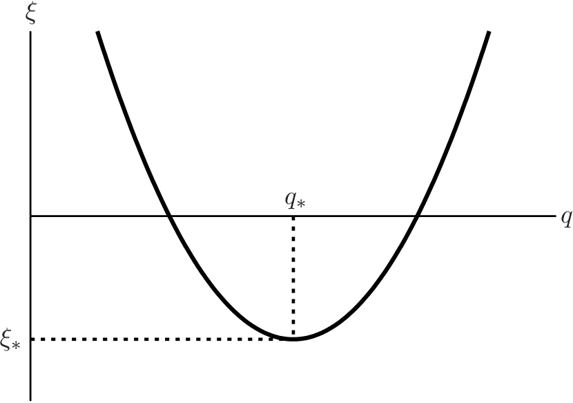
Figure 2: A cartoon of a typical neutral curve, showing the bifurcation point $(q_{\mathchoice{*}{\displaystyle*}{\textstyle*}{\scriptstyle*}},\,\xi_{\mathchoice{*}{\displaystyle*}{\textstyle*}{\scriptstyle*}})$. For the ITG model, $\xi=\Gamma^{2}$ [Eq. (12)], where $\xi=0$ is the linear threshold. For gyrokinetic particle noise, $\widehat{\xi}_{\mathchoice{*}{\displaystyle*}{\textstyle*}{\scriptstyle*}}<0$ with $|\widehat{\xi}_{\mathchoice{*}{\displaystyle*}{\textstyle*}{\scriptstyle*}}|=O({\mathcal{D}}_{\perp}^{-1})\ll 1$.

To be more precise, observe from Fig. 2 that at the point of bifurcation the neutral curve N has a minimum at a point $(q_{\mathchoice{*}{\displaystyle*}{\textstyle*}{\scriptstyle*}},\xi_{\mathchoice{*}{\displaystyle*}{\textstyle*}{\scriptstyle*}})$. By definition, N obeys

$$\widehat{\lambda}(q,\xi)=0,$$ (36)

which defines N as a function $\xi(q)$. From

$$\left(\frac{\partial\widehat{\lambda}}{\partial q\smash{\hbox to0.0pt{\;\;\;$\xi$\hss}}}\right)\phantom{\xi}\,dq+\left(\frac{\partial\widehat{\lambda}}{\partial\xi\smash{\hbox to0.0pt{\;\;\;$q$\hss}}}\right)\phantom{q}\,d\xi=0,$$ (37)

one finds that on N one has

$$\frac{d\xi}{dq}=-\frac{(\partial\widehat{\lambda}/\partial q)_{|\xi}}{(\partial\widehat{\lambda}/\partial\xi)_{|q}},$$ (38)

so at the bifurcation point where $N$ has a minimum one has

$$\left(\frac{\partial\widehat{\lambda}}{\partial q\smash{\hbox to0.0pt{\;\;\;$\xi$\hss}}}\right)\phantom{\xi}=0.$$ (39)

This condition and Eq. (36) provide two simultaneous equations to be solved for $q_{\mathchoice{*}{\displaystyle*}{\textstyle*}{\scriptstyle*}}$ and $\xi_{\mathchoice{*}{\displaystyle*}{\textstyle*}{\scriptstyle*}}$. Equation (36) is just

$$\det[\mathsf{\nu}^{\rm Z}+\textsf{m}(0)]=0,$$ (40)

where $\textsf{m}(0)\equiv\textsf{m}(\widehat{\lambda}{=}0,q,\xi)$. To simplify the condition (39), one can appeal to the Jacobi formula for the derivative of the determinant of a matrix A:

$$d\det(\textsf{A})=\mathop{\hbox{\rm tr}}\nolimits[\mathop{\hbox{\rm adj}}\nolimits(\textsf{A})\cdot d\textsf{A}],$$ (41)

where $\mathop{\hbox{\rm tr}}\nolimits$ denotes the trace and $\mathop{\hbox{\rm adj}}\nolimits$ denotes the adjugate, i.e., the transpose of the cofactor matrix. Upon differentiating Eq. (34) and enforcing Eq. (39), one obtains

$$0=\mathop{\hbox{\rm tr}}\nolimits\{\mathop{\hbox{\rm adj}}\nolimits[\mathsf{\nu}^{\rm Z}+\textsf{m}(0)]\cdot\partial q\,\textsf{m}(0)\}.$$ (42)

Solution of the simultaneous nonlinear equations Eq. (40) and (42) determine the bifurcation point $(q_{\mathchoice{*}{\displaystyle*}{\textstyle*}{\scriptstyle*}},\,\xi_{\mathchoice{*}{\displaystyle*}{\textstyle*}{\scriptstyle*}})$.

The elements of m are linear functions of the elements of C, and each of those elements is a linear function of the elements of the noise matrix D, which we take to scale with the common level parameter $\varepsilon$: $\textsf{D}=\varepsilon\overline{\nu}\widehat{\textsf{D}}$, where $\widehat{\textsf{D}}=O(1)$. Also let $\mathsf{\nu}^{\rm Z}=\eta\overline{\nu}\widehat{\mathsf{\nu}}^{\rm Z}$, where $\eta$ sets the common size of $\nu_{\zeta}^{\rm Z}$ and $\nu_{T}^{\rm Z}$ such that $\widehat{\mathsf{\nu}}^{\rm Z}=O(1)$. Since the elements of m are linearly proportional to those of D, it can be seen that the solution will depend only on the ratio $\overline{\varepsilon}\doteq\varepsilon/\eta$. Upon factoring $\eta^{n}$ from each of Eqs. (40) and (42), where $n=2$ for the ITG model, those equations become

$$0 =\det[\widehat{\mathsf{\nu}}^{\rm Z}+\textsf{m}(0,q_{\mathchoice{*}{\displaystyle*}{\textstyle*}{\scriptstyle*}},\widehat{\xi}_{\mathchoice{*}{\displaystyle*}{\textstyle*}{\scriptstyle*}};\overline{\varepsilon},\widehat{\textsf{D}})],$$ (43a)

$$0 =\mathop{\hbox{\rm tr}}\nolimits\{\mathop{\hbox{\rm adj}}\nolimits[\widehat{\mathsf{\nu}}^{\rm Z}+\textsf{m}(0,q_{\mathchoice{*}{\displaystyle*}{\textstyle*}{\scriptstyle*}},\widehat{\xi}_{\mathchoice{*}{\displaystyle*}{\textstyle*}{\scriptstyle*}};\overline{\varepsilon},\widehat{\textsf{D}})]\cdot\partial_{q_{\mathchoice{*}{\displaystyle*}{\textstyle*}{\scriptstyle*}}}\textsf{m}(0,q_{\mathchoice{*}{\displaystyle*}{\textstyle*}{\scriptstyle*}},\widehat{\xi}_{\mathchoice{*}{\displaystyle*}{\textstyle*}{\scriptstyle*}};\overline{\varepsilon},\widehat{\textsf{D}}).$$ (43b)

From Eq. (28), we see that near linear threshold the divergent elements of $\textsf{C}^{(0)}$ scale as $\textsf{D}/\overline{\nu}\widehat{\xi}=\eta(\overline{\varepsilon}/\widehat{\xi})\widehat{\textsf{D}}$. Therefore, one has

$$\textsf{m}(0,q_{\mathchoice{*}{\displaystyle*}{\textstyle*}{\scriptstyle*}},\widehat{\xi}_{\mathchoice{*}{\displaystyle*}{\textstyle*}{\scriptstyle*}};\overline{\varepsilon},\widehat{\textsf{D}})\approx\textsf{m}(0,q_{\mathchoice{*}{\displaystyle*}{\textstyle*}{\scriptstyle*}},\widehat{\xi}_{\mathchoice{*}{\displaystyle*}{\textstyle*}{\scriptstyle*}}/\overline{\varepsilon};\widehat{\textsf{D}}).$$ (44)

In the absence of additional small parameters in m, it is then clear that the solution for $(q_{\mathchoice{*}{\displaystyle*}{\textstyle*}{\scriptstyle*}},\,\widehat{\xi}_{\mathchoice{*}{\displaystyle*}{\textstyle*}{\scriptstyle*}}/\overline{\varepsilon})$ is $O(1)$, from which it follows that $\widehat{\xi}_{\mathchoice{*}{\displaystyle*}{\textstyle*}{\scriptstyle*}}=O(\overline{\varepsilon})$. In cases in which the forcing is due to turbulence and the zonal damping is weak, $\overline{\varepsilon}$ is large. Some analytical progress can be made by using isotropic ring forcing,Srinivasan and Young (2012) $\widehat{\textsf{D}}(k_{x},k_{y})\propto\delta(k-k_{\rm f})$. (ParkerParker and Krommes (2016) has used such forcing to show how the zonostrophic instability is a generalization of the modulational instability.) However, the situation is different when the forcing is due to discrete particle noise, as discussed next.

IV.2.2 Forcing due to particle discreteness

In a tokamak, the zonal damping rates are expected to be proportional to the ion–ion collision rateRosenbluth and Hinton (1998): $\eta\sim\nu_{ii}$. Built into that rate is the noise level $\epsilon$ due to ion discreteness. Therefore $\overline{\varepsilon}$ is independent of the basic noise level, specifically the plasma parameter $\epsilon_{p}$. However, it has been shownKrommes, Lee, and Oberman (1986); Nevins et al. (2005) that in magnetized, gyrokinetic plasma the thermal fluctuation level is reduced by the strong shielding effect of ion polarization, i.e., that level scales with the inverse of the perpendicular dielectric constant ${\mathcal{D}}_{\perp}$. Thus $\overline{\varepsilon}=O({\mathcal{D}}_{\perp}^{-1})\ll 1$. The particle-noise-driven zonostrophic bifurcation therefore occurs at

$$\widehat{\Gamma}_{0}^{2}=\widehat{\nu}_{\zeta}\widehat{\nu}_{T}-a\overline{\varepsilon},$$ (45)

where $a$ is a constant. Recall that all of $\widehat{\Gamma}_{0}^{2}$, $\widehat{\nu}_{\zeta}$, and $\widehat{\nu}_{T}$ are positive. To the extent that $\overline{\varepsilon}\ll\widehat{\nu}_{\zeta}\widehat{\nu}_{T}$, the bifurcation occurs essentially at the linear threshold. We understand this to define the onset of the Dimits-shift regime. For $\overline{\varepsilon}\gg\widehat{\nu}_{\zeta}\widehat{\nu}_{T}$, no zonostrophic instability occurs to the left of the linear threshold.

For a quantitative calculation, we recall the theory of gyrokinetic noise.Krommes, Lee, and Oberman (1986); Nevins et al. (2005) The general theory of statistical fluctuations in the presence of both particle discreteness and turbulence is complicatedRose (1979); some discussion is given in LABEL:JAK_noise. There are at least two qualitative issues. Most fundamentally, common statistical closures such as the DIA are incorrect because they make an assumption about Gaussian initial statistics that is incorrect in the presence of particle discretenessRose (1979) (this can easily be seen from the form of the thermal-equilibrium Gibbs distribution). Also, the details of discrete particle noise depend on the shape of the one-particle distribution function $f$. Fluid descriptions of the kind pursued in the present article assume that $f$ is a local Maxwellian. That is not unreasonable for the level of description to which we aspire here, particularly since there is no turbulence in the regimes of either linear stability or the Dimits shift, but it should be revisited in the regime where the particle noise is strongly amplified close to linear threshold. That is left for future work.

Thus we shall proceed as follows.

(i) For $\kappa=0$, we determine the equilibrium gyrokinetic noise level using the noise calculations of KrommesKrommes, Lee, and Oberman (1986) and Nevins et al.,Nevins et al. (2005) based on the Rostoker superposition principle. The latter calculations are more appropriate for the present case since they were done using the assumption of adiabatic electron response.

(ii) We infer the forcing functions by balancing the forcing against the Landau damping rates assumed in the basic ITG fluid mode, for given noise level. Thus, if a scalar random variable $\widetilde{\psi}$ obeys

$$\frac{d\widetilde{\psi}}{dt}+\nu\widetilde{\psi}={\widetilde{f}}(t),$$ (46)

where ${\widetilde{f}}(t)$ is Gaussian white noise with covariance $\langle\delta\!f(t)\delta\!f(t^{\prime})\rangle=2D\delta(t-t^{\prime})$, the steady-state solution for the second-order statistics of the Langevin equation (46) is

$$\langle\delta\psi^{2}\rangle=D/\nu.$$ (47)

Given $\langle\delta\widetilde{\psi}^{2}\rangle$, $D$ is determined as $\nu\langle\delta\widetilde{\psi}^{2}\rangle$. The determination of the $n$-dimensional forcing matrix D is a simple generalization of this result, as we shall explicate below.

(iii) Finally, now knowing D, we turn on $\kappa$ and proceed as in the earlier part of this article to calculate the noise-drive, $\kappa$-dependent fluctuation level and then the onset of the zonostrophic instability.

IV.2.3 Constraints on the damping coefficients; the forcing matrix

To carry out the above program, we first calculate the equilibrium correlation matrix $\textsf{C}^{(\rm eq)}\doteq\langle\delta{\bm{\psi}}\,\delta{\bm{\psi}}^{\dagger}\rangle^{(\rm eq)}$, where $\widetilde{{\bm{\psi}}}\doteq(\widetilde{\zeta},\,\widetilde{T})^{T}$. (We omit the dependence on ${\bm{k}}$ of this and the other quantities in the following discussion.) Because we work in the electrostatic approximation, both components of $\delta{\bm{\psi}}$ are driven by the random potential $\delta\varphi$. The vorticity is linearly related to $\delta\varphi$: $\delta\zeta={\mathcal{Z}}\delta\varphi$, where ${\mathcal{Z}}\doteq 1+{\overline{k}}^{2}$. The fluctuating temperature could in principle contain nonlinear contributions, but since we restrict ourselves to weak coupling, the linear approximation is adequate: $\delta T={\mathcal{T}}\delta\varphi$, where we shall calculate ${\mathcal{T}}$ from the equilibrium gyrokinetic equation below.

The fact that the vector $\delta{\bm{\psi}}$ is linearly proportional to the scalar $\delta\varphi$ has important consequences for the properties of the equilibrium correlation matrix. Let $\delta{\bm{\psi}}=\boldsymbol{{\mathcal{S}}}\,\delta\varphi$, where $\boldsymbol{{\mathcal{S}}}$ is an $n$-dimensional, non-zero scaling vector. [For our specific problem, we have $\boldsymbol{{\mathcal{S}}}=({\mathcal{Z}},\,{\mathcal{T}})^{T}$.] Thus $\textsf{C}^{(\rm eq)}=\boldsymbol{{\mathcal{S}}}\,\boldsymbol{{\mathcal{S}}}^{T}C_{\varphi\varphi}^{(\rm eq)}$. This matrix has one positive eigenvalue, $\lambda_{+}=\mathopen{\parallel}\boldsymbol{{\mathcal{S}}}\mathclose{\parallel}^{2}\doteq\boldsymbol{{\mathcal{S}}}^{\dagger}\cdot\boldsymbol{{\mathcal{S}}}$, with associated eigenvector ${\bm{e}}_{+}=\widehat{\boldsymbol{{\mathcal{S}}}}\doteq\boldsymbol{{\mathcal{S}}}/\mathopen{\parallel}\boldsymbol{{\mathcal{S}}}\mathclose{\parallel}$. The remaining $n-1$ eigenvalues vanish. This follows since $\widehat{\boldsymbol{{\mathcal{S}}}}$ can be taken to define the normal to an $(n-1)$-dimensional hyperplane; thus one can find $n-1$ vectors $\widehat{{\bm{q}}}_{i}$ ($i=2,\dots,n$) such that $\widehat{\boldsymbol{{\mathcal{S}}}}^{\dagger}\cdot\widehat{{\bm{q}}}_{i}=0$. It follows that $\textsf{C}^{(\rm eq)}$ is diagonalized by the unitary matrix $\textsf{U}\doteq({\bm{e}}_{+},\,\widehat{{\bm{q}}}_{2},\dots,\widehat{{\bm{q}}}_{n})$ according to

$$\overline{\textsf{C}}\doteq\textsf{U}^{\dagger}\cdot\textsf{C}\cdot\textsf{U}=\mathopen{\parallel}\boldsymbol{{\mathcal{S}}}\mathclose{\parallel}^{2}\begin{pmatrix}1&0&\dots&0\\ 0&0&\dots&0\\ \vdots&\vdots&\ddots&0\\ 0&0&\dots&0\end{pmatrix}C_{\varphi\varphi}^{(\rm eq)}.$$ (48)

We now want to work backwards and determine the associated forcing matrix D. The equilibrium Langevin equation

$$\frac{d\delta\widetilde{{\bm{\psi}}}}{dt}+\textsf{V}\cdot\delta\widetilde{{\bm{\psi}}}=\delta{\bm{f}},$$ (49)

where V contains the linear dissipation, transforms to

$$\frac{d\delta\overline{{\bm{\psi}}}}{dt}+\overline{\textsf{V}}\cdot\delta\overline{{\bm{\psi}}}=\delta\overline{{\bm{f}}},$$ (50)

where

$$\delta\overline{{\bm{\psi}}}\doteq\mathopen{\parallel}\boldsymbol{{\mathcal{S}}}\mathclose{\parallel}\begin{pmatrix}1\\ 0\\ \vdots\\ 0\end{pmatrix}\delta\varphi,\quad\delta\overline{{\bm{f}}}\doteq\mathopen{\parallel}\boldsymbol{{\mathcal{S}}}\mathclose{\parallel}\begin{pmatrix}1\\ 0\\ \vdots\\ 0\end{pmatrix}\delta\!f_{\varphi}$$ (51)

and $\overline{\textsf{V}}\doteq\textsf{U}^{\dagger}\cdot\textsf{V}\cdot\textsf{U}$. The fact that the time derivative and forcing appear only in the first component of Eq. (50) places restrictions on the form of the transformed dissipation matrix $\overline{\textsf{V}}$, and thus on the original V. Specifically, if V is taken to be diagonal, as we did in writing the model system Eq. (3), then one can show that the diagonal elements must be equal. To see this explicitly for $n=2$, suppose that

$$\overline{\textsf{V}}=\begin{pmatrix}a&b\\ c&d\end{pmatrix}.$$ (52)

The unitary transformation matrix (whose columns are the eigenvectors) can be chosen to be

$$\textsf{U}=\frac{1}{\Delta^{1/2}}\begin{pmatrix}{\mathcal{Z}}&-{\mathcal{T}}^{\mathchoice{*}{\displaystyle*}{\textstyle*}{\scriptstyle*}}\\ {\mathcal{T}}&{\mathcal{Z}}^{\mathchoice{*}{\displaystyle*}{\textstyle*}{\scriptstyle*}}\end{pmatrix},$$ (53)

where $\Delta\doteq|{\mathcal{Z}}|^{2}+|{\mathcal{T}}|^{2}=\mathopen{\parallel}\boldsymbol{{\mathcal{S}}}\mathclose{\parallel}^{2}$. With $\delta\overline{{\bm{\psi}}}=\textsf{U}^{\dagger}\cdot\delta{\bm{\psi}}$, this leads to the transformed Langevin equations

$$\frac{d\delta\varphi}{dt}+a\,\delta\varphi =\delta\!f_{\varphi},$$ (54a)

$$0+c\,\delta\varphi =0.$$ (54b)

Thus $c=0$, with $b$ and $d$ being arbitrary at this point. Upon transforming back, one finds

$$\textsf{V}=\begin{pmatrix}|{\mathcal{Z}}|^{2}a-{\mathcal{Z}}{\mathcal{T}}b+|{\mathcal{T}}|^{2}d&{\mathcal{Z}}{\mathcal{T}}^{\mathchoice{*}{\displaystyle*}{\textstyle*}{\scriptstyle*}}(a-d)+{\mathcal{Z}}^{2}b\\ {\mathcal{Z}}^{\mathchoice{*}{\displaystyle*}{\textstyle*}{\scriptstyle*}}{\mathcal{T}}(a-d)-{\mathcal{T}}^{2}b&|{\mathcal{T}}|^{2}a+{\mathcal{Z}}{\mathcal{T}}b+|{\mathcal{Z}}|^{2}d\end{pmatrix}.$$ (55)

The requirement that the off-diagonal elements vanish is easily seen to imply $b=0$ and $d=a$; thus $\textsf{V}=\overline{\textsf{V}}=a\textsf{I}$.

Upon replacing $a$ by the common damping rate $\nu=\widehat{\nu}_{\zeta}=\widehat{\nu}_{T}=\overline{\nu}$ and applying the result (47) to Eq. (54a), one determines

$$D_{\zeta\zeta}^{(\rm eq)}=\nu\langle|\delta\varphi|^{2}\rangle^{(\rm eq)}.$$ (56)

The back transformation $\delta{\bm{f}}=\textsf{U}\cdot\delta\overline{{\bm{f}}}$ leads to

$$\textsf{D}^{(\rm eq)}=\nu\textsf{C}^{(\rm eq)},$$ (57)

where

$$\textsf{C}^{(\rm eq)}=\begin{pmatrix}|{\mathcal{Z}}|^{2}&{\mathcal{Z}}{\mathcal{T}}^{\mathchoice{*}{\displaystyle*}{\textstyle*}{\scriptstyle*}}\\ {\mathcal{Z}}^{\mathchoice{*}{\displaystyle*}{\textstyle*}{\scriptstyle*}}{\mathcal{T}}&|{\mathcal{T}}|^{2}\end{pmatrix}C_{\varphi\varphi}^{(\rm eq)}.$$ (58)

IV.2.4 The scaling coefficients

To determine the scaling coefficient ${\mathcal{T}}$, we solve the gyrokinetic equation linearized (denoted by $\Delta$) around thermal equilibrium,

$$\frac{\partial\Delta F}{\partial t}+v_{\parallel}\nabla_{\parallel}\Delta F+\frac{q}{m}\Delta E_{\parallel}\frac{\partial F_{\rm M}}{\partial v_{\parallel}}=0$$ (59)

to find

$$\Delta F_{i}({{\bm{k}},\omega})=Z\tau^{-1}\left(\frac{k_{\parallel}v_{\parallel}}{\omega-k_{\parallel}v_{\parallel}+i\epsilon}\right)\Delta\varphi({{\bm{k}},\omega})F_{{\rm M}i},$$ (60)

where $Z$ is the atomic number and $\tau\doteq T_{i}/T_{e}$. The fluctuating temperature is then

$$\Delta T_{i}=\int\!d{\bm{v}}\,\left(\frac{1}{2}m_{i}v^{2}-\frac{3}{2}T_{i}\right)\Delta F_{i}.$$ (61)

Since we ignore FLR effects, the perpendicular part of $\mathchoice{{\textstyle\frac{1}{2}}}{{\textstyle\frac{1}{2}}}{{\scriptstyle\frac{1}{2}}}{{\scriptscriptstyle\frac{1}{2}}}v^{2}-\frac{3}{2}=(\mathchoice{{\textstyle\frac{1}{2}}}{{\textstyle\frac{1}{2}}}{{\scriptstyle\frac{1}{2}}}{{\scriptscriptstyle\frac{1}{2}}}v_{\parallel}^{2}-\mathchoice{{\textstyle\frac{1}{2}}}{{\textstyle\frac{1}{2}}}{{\scriptstyle\frac{1}{2}}}{{\scriptscriptstyle\frac{1}{2}}})+(\mathchoice{{\textstyle\frac{1}{2}}}{{\textstyle\frac{1}{2}}}{{\scriptstyle\frac{1}{2}}}{{\scriptscriptstyle\frac{1}{2}}}v_{\perp}^{2}-1)$ integrates away. For the parallel part, it is conventional in standard drift-wave theory to look for modes with $\omega\gg k_{\parallel}v_{{t}i}$. Upon expanding the denominator for small $k_{\parallel}v_{\parallel}/\omega$, one finds

$${\mathcal{T}}({{\bm{k}},\omega})\doteq\Delta\varphi^{-1}({{\bm{k}},\omega})\left(\frac{\Delta T_{i}({{\bm{k}},\omega})}{T_{i}}\right)\approx Z\tau^{-1}\frac{k_{\parallel}^{2}v_{{t}i}^{2}}{\omega^{2}}\ll 1.$$ (62)

Unfortunately, this expansion is not well justified for the ITG mode. However, one can already see another issue, which is that any such ${\mathcal{T}}$, calculated with or without expansion, will depend on $\omega$. This goes beyond the level of detail assumed in the above white-noise calculations, which assume that the scaling coefficients depended only on ${\bm{k}}$. In problems for which the linear eigenfrequency is dominantly real, this difficulty can be justifiably surmounted by replacing $\omega$ by the real mode frequency $\Omega_{\bm{k}}$. When $\omega$ is purely imaginary, this procedure is less justified, and to properly deal with the fact that $|\omega|\sim k_{\parallel}v_{{t}i}$, one should do a kinetic analysis. Alternatively, qualitatively correct results should obtain by ignoring ${\mathcal{T}}$ altogether, thus forcing only the vorticity.

IV.2.5 The gyrokinetic noise level

As a trivial modification of the work of Nevins et al.,Nevins et al. (2005) one finds for the case of ITG modes with adiabatic electrons Krommes (2007) the fluctuating noise level

$$\frac{\langle\delta\phi\,\delta\phi\rangle({\bm{k}})}{8\pi}=\frac{T_{\mathrm{i0}}/2}{\epsilon_{\rm GV}({\bm{k}})}\left(\frac{k_{{D}i}^{2}\Gamma(k_{\perp}^{2}\rho_{i}^{2})/k_{D}^{2}}{k^{2}(1+\epsilon_{\rm GV}^{-1}k_{{D}e}^{2}/k^{2})(1+k^{2}\lambda_{D}^{2})}\right).$$ (63)

Here $k_{{D}s}$ is the Debye length for species $s$, $k_{D}^{2}\doteq k_{{D}e}^{2}+k_{{D}i}^{2}$, $\Gamma(b)\doteq I_{0}(b)e^{-b}$, and the dielectric permittivity of the gyrokinetic vacuum $\epsilon_{\rm GV}$ is given by

$$\epsilon_{\rm GV}\approx 1+\left(\frac{k_{{D}i}^{2}}{k^{2}}\right)(1-\Gamma).$$ (64)

In our normalized variables we have

$$\mathsf{C}^{(\mathrm{eq})}_{\varphi\varphi}(k_{x},k_{y})=\int\frac{dk_{z}}{2\pi}\frac{1}{n_{i}}\left(\frac{\tau{\mathcal{D}}_{\perp}}{\epsilon_{\rm GV}}\right)$$

$$\quad\times\left(\frac{\Gamma(\tau k_{\perp}^{2})}{\rho_{*}^{2}k^{2}(1+\epsilon_{\rm GV}^{-1}{\mathcal{D}}_{\perp}/k^{2})(1+\tau+\tau k^{2}/{\mathcal{D}}_{\perp})}\right)$$ (65)

with

$$\epsilon_{\rm GV}\approx 1+\left(\frac{{\mathcal{D}}_{\perp}}{\tau k^{2}}\right)[1-\Gamma(\tau k^{2})].$$ (66)

Here, $\rho_{*}\doteq\rho_{\textrm{s}}/a$, $\tau\doteq T_{\mathrm{i0}}/T_{\mathrm{e0}}$, ${\mathcal{D}}_{\perp}\doteq\omega_{{p}i}^{2}/\omega_{{c}i}^{2}$, and $n_{i}$ denotes the ion density scaled by $\rho_{\textrm{s}}^{3}$. The zonostrophic instability problem is thus specified in terms of the parameters $n_{i}$, $\rho_{*}$, $\tau$ and ${\mathcal{D}}_{\perp}$. In the gyrokinetic regimeKrommes, Lee, and Oberman (1986) ${\mathcal{D}}_{\perp}\gg 1$, so in the cold-ion limit one has $\lim_{\tau\to 0}\epsilon_{\rm GV}\approx{\mathcal{D}}_{\perp}$.

IV.3 Solution of the neutral curve equation

A representative, numerically calculated neutral curve is displayed in Fig. 3. It displays the expected qualitative features, including a critical zonal wave number $q_{{\mathchoice{*}{\displaystyle*}{\textstyle*}{\scriptstyle*}}}$, a supercritical bifurcation, and a parabolic shape near onset. Notice that the zonostrophic instability sets in for $q_{{\mathchoice{*}{\displaystyle*}{\textstyle*}{\scriptstyle*}}}\rho_{\textrm{s}}=O(1)$, not $q_{{\mathchoice{*}{\displaystyle*}{\textstyle*}{\scriptstyle*}}}/k\ll 1$.

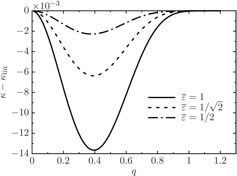
Figure 3: A a series of representative neutral curves for various values of $\overline{\varepsilon}$, calculated numerically for the gyrokinetic noise spectrum given by Nevins et al.Nevins et al. (2005) for $\tau=1$, $\rho_{*}=0.3$, $n_{i}=1$, ${\mathcal{D}}_{\perp}=100$, ${\mathcal{T}}=0$ and $\nu=|k_{y}|$ represents damping in a Landau-fluid closure. Curves are quantitatively similar for ${\mathcal{T}}=-0.25$.

Our principal purpose in displaying a numerically calculated neutral curve is to demonstrate that our analytically derived dispersion relation is robust and that no unexpected pathologies arise. Clearly the entire model is extremely crude, so our results cannot be quantitatively compared with experiments or fully kinetic simulations.

Missing from Fig. 3 is an inner, secondary stability curve for the steady zonal solutions that emerge above the point of zonostrophic instability. The existence of that boundary is known from previous work, including most recently that of Parker and Krommes,Parker and Krommes (2013, 2014) who calculated it numerically for the case of the modified Hasegawa–Mima equation. Calculation of that curve for the present model requires numerical work and is beyond the scope of this paper.

V Discussion

In summary, we have used the CE2 stochastic model to derive the dispersion relation of the noise-driven zonostrophic instability for a simple two-field model of the ion-temperature-gradient-driven mode, and we have numerically calculated the neutral curve and found the first unstable zonal mode for a representative noise spectrum.

The principal goal of this work is to present a new interpretation of the zonostrophic instability as being driven by discrete particle noise instead of the more conventional interpretation as being due to coupling to extrinsic turbulence. While it is obvious that in realistic tokamak microturbulence there is a plethora of modes in addition to the ITG mode, coupling to those modes should not be necessary for a self-consistent description of the behavior of the ITG mode itself as $\kappa$ (the normalized magnitude of the temperature gradient) is increased. We have shown that such a self-consistent description is possible when discrete particle noise is included. By introducing that noise, one is able to “open up” the zonostrophic bifurcation that introduces the onset of the Dimits-shift regime, which we have shown occurs just slightly below the linear threshold.

Left undone is the extension of these results through the right-hand boundary of the Dimits shift. This requires addressing the secondary stability boundary of the steady zonal flows that emerge from the zonostrophic bifurcation. If our interpretation is to be consistent with the known behavior observed in the simulations, that stability curve must close off for sufficiently large $\kappa$. Such behavior — the so-called Busse balloon — is known to occur for the closely analogous problem of Rayleigh–Benard thermal convection.Busse (1967); Busse and Whitehead (1971) Pursuing this investigation would augment current understanding of the Dimits shift and would provide a bridge between the sometimes arcane specialty of plasma physics and a large and broad literature on bifurcation phenomena in physical systems.

Appendix A Realizability of the homogeneous solution

The CE2 closure deals only with first- and second-order statistics. Assuming Gaussian forcing, the multivariate PDF of $\widetilde{\varphi}$ and $\widetilde{T}$ is a 2D Gaussian. Realizability of the steady-state solution for a nonsingular PDF requires that

$$\textsf{C}^{(0)}\doteq\begin{pmatrix}C_{\varphi\varphi}^{(0)}&C_{\varphi T}^{(0)}\\ C_{\varphi T}^{(0)}{}^{\mathchoice{*}{\displaystyle*}{\textstyle*}{\scriptstyle*}}&C_{TT}^{(0)}\end{pmatrix}$$ (67)

is positive definite for all realizable forcings. For a matrix to be positive definite, Sylvester’s criterion states that its leading principal minor determinants must be positive. Thus in the absence of any constraints on the forcing, one must satisfy

$$C_{\varphi\varphi}>0,\quad\Delta\doteq C_{\varphi\varphi}^{(0)}C_{TT}^{(0)}-|C_{\varphi T}^{(0)}|^{2}>0.$$ (68)

If no mistakes have been made, realizability is guaranteed up to the linear threshold because the covariance matrix has been derived from a set of primitive amplitude equations driven by realizable random forcings; above threshold, a homogeneous steady state does not exist. As a partial check, we consider the case with $D_{\zeta T}^{\prime\prime}=0$. Then from Eq. (28) one finds that

$$C_{\varphi\varphi}^{(0)}=(2\overline{\nu}{\overline{k}}^{4}\widehat{\xi})^{-1}[(\widehat{\xi}^{2}-\widehat{\nu}_{T}^{2})D_{\zeta\zeta}-k_{y}^{2}\widehat{\epsilon}^{2}D_{TT}].$$ (69)

For $\xi<0$ (linear stability), this is easily seen to be positive.

In terms of the real vector ${\bm{D}}\doteq(D_{\zeta\zeta},\,D_{TT},\,D_{\zeta T}^{\prime})^{T}$, the evaluation of $\Delta$ for $D_{\zeta T}^{\prime\prime}=0$ leads to the quadratic form $F_{3}={\bm{D}}^{T}\cdot\textsf{S}_{3}\cdot{\bm{D}}$, where for this case

$$\textsf{S}_{3}=\begin{pmatrix}a&b&0\\ b&d&0\\ 0&0&f\end{pmatrix};$$ (70)

thus $F_{3}=aD_{\zeta\zeta}^{2}+2bD_{\zeta\zeta}D_{TT}+d\,D_{TT}^{2}+fD_{\zeta T}^{\prime 2}$ and the coefficients $a$, $b$, $d$, and $f$ can be obtained from Eqs. (27) and (28). After some algebra, one finds

$$a =C(\overline{\nu}|\xi|)^{-1}(-k_{y}^{2}\kappa^{2}\xi),$$ (71a)

$$b =C(\overline{\nu}|\xi|)^{-1}{\overline{k}}^{4}\left[\xi-\mathchoice{{\textstyle\frac{1}{2}}}{{\textstyle\frac{1}{2}}}{{\scriptstyle\frac{1}{2}}}{{\scriptscriptstyle\frac{1}{2}}}(\widehat{\nu}_{\zeta}^{2}+\widehat{\nu}_{T}^{2})\right]\xi,$$ (71b)

$$d =C(\overline{\nu}|\xi|)^{-1}{\overline{k}}^{4}(-k_{y}^{2}\epsilon^{2}\xi),$$ (71c)

$$f =-(\overline{\nu}{\overline{k}}^{2})^{-1},$$ (71d)

where $C\doteq(2{\overline{k}}^{4})^{-1}$. In the region of linear stability ($\xi<0$), we observe that $a$, $b$, and $d$ are positive, while $f<0$. The criteria that $F_{3}$ be positive definite are

$$a>0,\quad\Delta_{2}\doteq ad-b^{2}>0,\quad\Delta_{3}\doteq\Delta_{2}f>0.$$ (72)

After more algebra, one finds

$$\Delta_{2}=C^{2}[\widehat{\xi}-(\widehat{\nu}_{\zeta}-\widehat{\nu}_{T})^{2}]<0,$$ (73)

and then $\Delta_{3}>0$. Thus the submatrix related to $D_{\zeta\zeta}$ and $D_{TT}$ violates unconstrained positive definiteness. However, realizabiity constrains $D_{\zeta\zeta}$ and $D_{TT}$ to be positive. Since all of $a$, $b$ and $d$ are positive, the subform $F_{2}$ is positive. We have thus verified that C is realizable for realizable forcing (for the special case $D_{\zeta T}^{\prime\prime}=0$).

To interpret the fact that $\Delta_{2}<0$, note that the eigenvalues of $\textsf{S}_{2}$ are $\lambda=\Sigma\pm(\Sigma^{2}-4\Delta_{2})^{1/2}$, where $\Sigma\doteq a+d>0$. Thus one eigenvalue is negative. The associated eigenvector satisfies $D_{TT}=-b^{-1}(a-\lambda_{-})D_{\zeta\zeta}<0$. Such an unrealizable forcing would violate the condition that the cross-correlation coefficient between $\delta\varphi$ and $\delta T$ must be less than 1 in absolute value.

Appendix B Details of the dispersion relation

For all $\nu$’s equal, the matrix $\widehat{\textsf{M}}$ and source vectors introduced in Eq. (31) have the form

$$\widehat{\textsf{M}}\doteq\begin{pmatrix}-(\widehat{\lambda}+2)\overline{h}_{+}^{2}\overline{h}_{-}^{2}&-ik_{y}\widehat{\epsilon}\overline{h}_{+}^{2}&ik_{y}\widehat{\epsilon}\overline{h}_{-}^{2}&0\\ -ik_{y}\widehat{\kappa}\overline{h}_{+}^{2}&(\widehat{\lambda}+2)\overline{h}_{+}^{2}&0&-ik_{y}\widehat{\epsilon}\\ ik_{y}\widehat{\kappa}\overline{h}_{-}^{2}&0&(\widehat{\lambda}+2\overline{\nu})\overline{h}_{-}^{2}&ik_{y}\widehat{\epsilon}\\ 0&-ik_{y}\widehat{\kappa}&ik_{y}\widehat{\kappa}&-(\widehat{\lambda}+2)\end{pmatrix},$$ (74)

$$\widehat{{\bm{s}}}_{U}\doteq\frac{ik_{y}}{\nu}\begin{pmatrix}\overline{h}_{+}^{2}(\overline{h}_{+}^{2}-q^{2})C_{\varphi\varphi}^{(+)}-\overline{h}_{-}^{2}(\overline{h}_{-}^{2}-q^{2})C_{\varphi\varphi}^{(-)}\\ -\overline{h}_{+}^{2}C_{\varphi T}^{(+)}+(\overline{h}_{-}^{2}-q^{2})C_{\varphi T}^{(-)}\\ -[-\overline{h}_{-}^{2}C_{T\varphi}^{(-)}+(\overline{h}_{+}^{2}-q^{2})C_{T\varphi}^{(+)}]\\ C_{TT}^{(+)}-C_{TT}^{(-)}\end{pmatrix},\quad\widehat{{\bm{s}}}_{T}\doteq\frac{k_{y}q}{\nu}\begin{pmatrix}0\\ -\overline{h}_{+}^{2}C_{\varphi\varphi}^{(+)}\\ \overline{h}_{-}^{2}C_{\varphi\varphi}^{(-)}\\ -(C_{\varphi T}^{(-)}-C_{T\varphi}^{(+)})\end{pmatrix}.$$ (75)

For the formalism to make sense, $\widehat{\textsf{M}}$ must be invertible, i.e., its determinant must not vanish. One finds

$$\Delta\doteq\det{\widehat{\textsf{M}}}=\overline{h}_{+}^{4}\overline{h}_{-}^{4}(\widehat{\lambda}+2)^{4}-2\overline{h}_{+}^{2}\overline{h}_{-}^{2}(\overline{h}_{+}^{2}+\overline{h}_{-}^{2})(\widehat{\xi}+1)(\widehat{\lambda}+2)^{2}+(\overline{h}_{+}^{2}-\overline{h}_{-}^{2})^{2}(\widehat{\xi}+1)^{2}.$$ (76)

There is no requirement that $\Delta$ be positive definite; one needs only that it not vanish at the point of zonostrophic bifurcation $\widehat{\lambda}=0$. This is not expected since $\widehat{\xi}_{\mathchoice{*}{\displaystyle*}{\textstyle*}{\scriptstyle*}}$ depends on the zonal-flow damping rates, which do not appear in $\widehat{\textsf{D}}$. Some general properties of $\Delta(\widehat{\xi},q)\equiv\Delta(\widehat{\lambda}=0,\widehat{\xi},q)$ are easy to determine. It can be shown to depend only on $q^{2}$. For $\widehat{\xi}=-1$, one has

$$\Delta(-1,q)=16\overline{h}_{+}^{4}\overline{h}_{-}^{4}>0.$$ (77)

$\Delta$ has a minimum with respect to $\widehat{\xi}$ at

$$\widehat{\xi}=\frac{4\overline{h}_{+}^{2}+\overline{h}_{-}^{2}(\overline{h}_{+}^{2}+\overline{h}_{-}^{2})}{{\overline{k}}^{2}(\overline{h}_{+}^{2}-\overline{h}_{-}^{2})^{4}}>0.$$ (78)

Its derivative at the linear threshold $\widehat{\xi}=0$ is

$$\frac{\partial\Delta(\widehat{\xi},q)}{\partial\widehat{\xi}}{}_{\big{|}\widehat{\xi}=0}=-i{\overline{k}}^{2}\overline{h}_{+}^{2}\overline{h}_{-}^{2}(\overline{h}_{+}^{2}+\overline{h}_{-}^{2})<0$$ (79)

and its second derivative is

$$\frac{\partial^{2}\Delta}{\partial\widehat{\xi}^{2}}=2{\overline{k}}^{4}(\overline{h}_{+}^{2}-\overline{h}_{-}^{2})^{2}>0.$$ (80)

$\Delta(0,q)$ vanishes for $q=0$ ($\overline{h}_{+}^{2}=\overline{h}_{-}^{2}={\overline{k}}^{2}$), and its derivative with respect to $q^{2}$ is

$$\frac{\partial\Delta(0,q)}{\partial q^{2}}=-12k_{x}^{2}{\overline{k}}^{4}<0.$$ (81)

Thus except for $q=0$ the determinant is negative at the linear threshold. Given that the second $\widehat{\xi}$ derivative is uniformly positive, one concludes that $\Delta$ must change sign somewhere in the stable region.

The dispersion relation can be simplified by using the transformation $C_{ij}^{(\pm)}(k_{x},k_{y})=C_{ji}^{(\mp)}(-k_{x},-k_{y})$. Once all equilibria are expressed at a single point $(k_{x}-q/2,k_{y})$, the transformation $k_{x}\rightarrow k_{x}+q/2$ is then performed. After defining

$$\overline{h} \doteq{\overline{k}}^{2}+2k_{x}q+q^{2},$$

$$\Omega \doteq k_{y}^{2}\epsilon\kappa(\overline{k}^{2}+\overline{h}^{2})-(\lambda+2\nu)^{2}\overline{k}^{2}\overline{h}^{2},$$

$$\Gamma_{k} \doteq\Omega-2k_{y}^{2}\kappa\epsilon\overline{k}^{2},$$

$$\Gamma_{h} \doteq\Omega-2k_{y}^{2}\kappa\epsilon\overline{h}^{2},$$

one finds that the determinant can be written as

$$\Delta^{\prime}\doteq\Omega^{2}-4k_{y}^{2}\epsilon^{2}\kappa^{2}\overline{k}^{2}\overline{h}^{2}$$ (82)

and the dispersion relation becomes

$$(\lambda+\nu_{\zeta}^{\mathrm{Z}}-iqB)(\lambda+\nu_{T}^{\mathrm{Z}}-qD)-iq^{2}AC=0,$$ (83)

where

$$A \doteq iq\epsilon\int\frac{dk_{x}\,dk_{y}}{(2\pi)^{2}}\,(k_{x}+q/2)k_{y}^{3}\overline{k}^{2}\Delta^{\prime}[\Gamma_{h}C_{\varphi\varphi}^{(0)}+2i\epsilon k_{y}\overline{h}^{2}(\lambda+2\nu)C_{\varphi T}^{(0)}],$$

$$B \doteq 2i\int\frac{dk_{x}\,dk_{y}}{(2\pi)^{2}}\,(k_{x}+q/2)k_{y}^{2}\Delta^{\prime}[\Omega(\lambda+2\nu)\overline{k}^{2}(\overline{k}^{2}-q^{2})C_{\varphi\varphi}^{(0)}-2k_{y}^{2}\epsilon^{2}(\lambda+2\nu)\overline{k}^{2}\overline{h}^{2}C_{TT}^{(0)}$$

$$\qquad\qquad-ik_{y}\epsilon\Gamma_{k}(\overline{k}^{2}-q^{2})C_{\varphi T}^{(0)}+ik_{y}\epsilon\overline{k}^{2}\Gamma_{h}C_{T\varphi}^{(0)}],$$

$$C \doteq 2\int\frac{dk_{x}\,dk_{y}}{(2\pi)^{2}}\,k_{y}^{2}\Delta^{\prime}[-2\kappa(\lambda+2\nu)^{2}k_{y}\overline{k}^{4}\overline{h}^{2}(\overline{k}^{2}-q^{2})C_{\varphi\varphi}^{(0)}+k_{y}\epsilon(\overline{h}^{2}\Gamma_{k}+\overline{k}^{2}\Gamma_{h})C_{TT}^{(0)}$$

$$\qquad\qquad+i(\lambda+2\nu)\overline{k}^{2}\overline{h}^{2}\Gamma_{k}C_{T\varphi}^{(0)}-i(\lambda+2\nu)\overline{k}^{2}(\overline{k}^{2}-q^{2})\Gamma_{h}C_{\varphi T}^{(0)}],$$

$$D \doteq q\int\frac{dk_{x}\,dk_{y}}{(2\pi)^{2}}\,k_{y}^{2}\Delta^{\prime}[(\lambda+2\nu)\overline{k}^{2}\overline{h}^{2}\Gamma_{k}C_{\varphi\varphi}^{(0)}-ik_{y}\epsilon(\overline{h}^{2}\Gamma_{k}+\overline{k}^{2}\Gamma_{h})C_{\varphi T}^{(0)}].$$

For $\mathcal{Z}\mathcal{T}^{*}=\pm\mathcal{Z}^{*}\mathcal{T}$ and $D_{ij}(k_{x},k_{y})=D_{ji}(k_{x},-k_{y})$, the dispersion relation is real-valued. If either $\mathcal{Z}$ or $\mathcal{T}$ are set to zero, then $A=C=0$ identically. In order for the dispersion relation to be satisfied, one must then solve

$$(\lambda+\nu_{\zeta}^{\mathrm{Z}}-iqB)(\lambda+\nu_{T}^{\mathrm{Z}}-qD)=0.$$ (84)

One can recover the dispersion relation found by Parker Parker and Krommes (2014) in the flat-density limit ($\beta=0$ in that reference) by forcing only the vorticity ($\mathcal{T}$ = 0), turning off the linear coupling terms ($\kappa=\epsilon=0$), and solving for the first branch $\lambda+\nu_{\zeta}^{\mathrm{Z}}-iqB=0$.

References

- Srinivasan and Young (2012) K. Srinivasan and W. R. Young, J. Atmos. Sci. 69, 1633 aggaa } (2012).
- Farrell and Ioannou (2015) B. F. Farrell and P. J. Ioannou, in Zonal Jets, edited by B. Galperin and P. Read (Cambridge University Press, Cambridge, 2015) Chap. V.2.2, in press.
- Tobias, Dagon, and Marston (2011) S. M. Tobias, K. Dagon, and J. B. Marston, Astrophys. J. 727, 127 aggaa } (2011).
- Tobias and Marston (2013) S. M. Tobias and J. B. Marston, Phys. Rev. Lett. 110, 104502 (2013).
- Marston, Qi, and Tobias (2016) J. B. Marston, W. Qi, and S. M. Tobias, in Zonal Jets, edited by B. Galperin and P. Read (Cambridge University Press, Cambridge, 2016) Chap. V.1.2, in press.
- Farrell and Ioannou (2003) B. F. Farrell and P. J. Ioannou, J. Atmos. Sci. 60, 2101 aggaa } (2003).
- Farrell and Ioannou (2009) B. F. Farrell and P. J. Ioannou, Phys. Plasmas 16, 112903 (2009).
- Krommes (2015) J. A. Krommes, J. Plasma Phys. 81, 1 aggaa } (2015).
- Kadomtsev (1965) B. B. Kadomtsev, Plasma Turbulence (Academic, New York, 1965) translated by L. C. Ronson from Problems in Plasma Theory, Vol. 4, edited by M. A. Leontovich (Atomizdat, Moscow, 1964) pp. 188–339. Translation edited by M. C. Rusbridge.
- Krommes (2002) J. A. Krommes, Phys. Rep. 360, 1 aggaa } (2002).
- Dimits et al. (2000) A. M. Dimits, G. Bateman, M. A. Beer, B. I. Cohen, W. Dorland, G. W. Hammett, C. Kim, J. E. Kinsey, M. Kotschenreuther, A. H. Kritz, L. L. Lao, J. Mandrekas, W. M. Nevins, S. E. Parker, A. J. Redd, D. E. Shumaker, R. Sydora, and J. Weiland, Phys. Plasmas 7, 969 aggaa } (2000).
- Rogers, Dorland, and Kotschenreuther (2000) B. N. Rogers, W. Dorland, and M. Kotschenreuther, Phys. Rev. Lett. 85, 5336 aggaa } (2000).
- Kolesnikov and Krommes (2005a) R. A. Kolesnikov and J. A. Krommes, Phys. Rev. Lett. 94, 235002 (2005a).
- Kolesnikov and Krommes (2005b) R. A. Kolesnikov and J. A. Krommes, Phys. Plasmas 12, 122302 (2005b).
- Note (1) An introductory review article on gyrokinetics that contains references to more specialized reviews and original papers is by J. A. Krommes, Annu. Ref. Fluid Mech.44, 175 (2012).
- Krommes, Lee, and Oberman (1986) J. A. Krommes, W. W. Lee, and C. Oberman, Phys. Fluids 29, 2421 aggaa } (1986).
- Nevins et al. (2005) W. M. Nevins, G. W. Hammett, A. M. Dimits, W. Dorland, and D. E. Shumaker, Phys. Plasmas 12, 122305 (2005).
- Parker and Krommes (2013) J. B. Parker and J. A. Krommes, Phys. Plasmas 20, 100703 (2013).
- Parker and Krommes (2014) J. B. Parker and J. A. Krommes, New J. Phys. 16, 035006 (2014).
- Parker and Krommes (2016) J. B. Parker and J. A. Krommes, in Zonal Jets, edited by B. Galperin and P. Read (Cambridge University Press, Cambridge, 2016) Chap. V.2.4, in press.
- Chen and Cheng (1980) L. Chen and C. Z. Cheng, Phys. Fluids 23, 2242 aggaa } (1980).
- Ottaviani et al. (1990) M. Ottaviani, F. Romanelli, R. Benzi, M. Briscolini, P. Santangelo, and S. Succi, Phys. Fluids B 2, 67 (1990).
- Hammett et al. (1993) G. W. Hammett, M. A. Beer, W. Dorland, S. C. Cowley, and S. A. Smith, Plasma Phys. Control. Fusion 35, 973 aggaa } (1993).
- Candy and Waltz (2003) J. Candy and R. E. Waltz, Phys. Rev. Lett. 91, 045001 (4 pages) (2003).
- Biglari, Diamond, and Rosenbluth (1989) H. Biglari, P. H. Diamond, and M. N. Rosenbluth, Phys. Fluids B 1, 109 (1989).
- Romanelli and Briguglio (1990) F. Romanelli and S. Briguglio, Phys. Fluids B 2, 754 (1990).
- Ottaviani et al. (1997) M. Ottaviani, M. Beer, S. Cowley, W. Horton, and J. Krommes, Phys. Rep. 283, 121 aggaa } (1997).
- Krommes and Parker (2015) J. A. Krommes and J. B. Parker, in Zonal Jets, edited by B. Galperin and P. Read (Cambridge University Press, Cambridge, 2015) Chap. V.1.1, in press.
- Kraichnan (1959) R. H. Kraichnan, J. Fluid Mech. 5, 497 aggaa } (1959).
- Leith (1971) C. E. Leith, J. Atmos. Sci. 28, 145 aggaa } (1971).
- Kraichnan (1970) R. H. Kraichnan, J. Fluid Mech. 41, 189 aggaa } (1970).
- Kraichnan (1971) R. H. Kraichnan, J. Fluid Mech. 47, 513 aggaa } (1971).
- Note (2) In this paper we use the standard plasma-physics slab coordinate system in which represents the direction of inhomogeneity (the radial coordinate in a tokamak) and represents the zonal direction (the poloidal direction in a tokamak). (In detail, in an actual tokamak the zonal flows are in the direction perpendicular to both and , i.e., mostly in the poloidal direction for large aspect ratio.) In geophysics, the roles of and are interchanged.
- (34) D. E. Ruiz, J. B. Parker, E. L. Shi, and I. Y. Dodin, “Two corrections to the drift-wave kinetic equation in the context of zonal-flow physics,” submitted.
- Cross and Greenside (2009) M. Cross and H. S. Greenside, Pattern Formation and Dynamics in Nonlinear Systems (Cambridge University Press, Cambridge, 2009).
- Rosenbluth and Hinton (1998) M. N. Rosenbluth and F. L. Hinton, Phys. Rev. Lett. 80, 724 aggaa } (1998).
- Rose (1979) H. A. Rose, J. Stat. Phys. 20, 415 aggaa } (1979).
- Krommes (2007) J. A. Krommes, Phys. Plasmas 14, 090501 (2007).
- Note (3) For many references to the DIA, see the review article (Ref. \rev@citealpnumJAK_PR) and tutorial article (Ref. \rev@citealpnumJAK_tutorial) by the second author.
- Note (4) When is the random velocity of a Brownian test particle of mass in a thermal bath of temperature , Eq. (47) leads to the Einstein relation , where is the velocity-space diffusion coefficient.
- Busse (1967) F. H. Busse, J. Math. Phys. 46, 146 aggaa } (1967).
- Busse and Whitehead (1971) F. H. Busse and J. A. Whitehead, J. Fluid Mech. 47, 305 aggaa } (1971).
- Note (5) Strictly speaking, realizability only requires positive semidefiniteness. Sylvester’s criterion is then that all of the principal minor determinants must be non-negative.