Latitude and power characteristics
of solar activity
in the end of the Maunder minimum

Abstract

Two important sources of information about sunspots in the Maunder minimum are the Spörer catalog [1] and observations of the Paris observatory [2], which cover in total the last quarter of the 17th and the first two decades of the 18th century.

These data, in particular, contain information about sunspot latitudes. As we showed in [3, 4], dispersions of sunspot latitude distributions are tightly related to sunspot indices, so we can estimate the level of solar activity in this epoch by a method which is not based on direct calculation of sunspots and is weakly affected by loss of observational data.

The latitude distributions of sunspots in the time of transition from the Maunder minimum to the common regime of solar activity proved to be wide enough. It gives evidences in favor of, first, not very low cycle No. $-3$ (1712–1723) with the Wolf number in maximum $\mbox{W}=100\pm 50$, and, second, nonzero activity in the maximum of cycle No. $-4$ (1700–1711) $\mbox{W}=60\pm 45$.

Therefore, the latitude distributions in the end of the Maunder minimum are in better agreement with the traditional Wolf number and new revisited indices of activity SN and GN [5, 6] than with the GSN [7]; the latter provide much lower level of activity in this epoch.

1 Introduction

The epoch of the Maunder minimum (MM) [8] lasted, as it is traditionally believed, since the middle of the 17th to the beginning of the third decade of the 18th century. It was very special in a low level of solar activity as well as its eminent hemisphere asymmetry. Now nobody doubts that the activity of the Sun in this epoch was low; however, it is still discussed how low it was (see, e.g., [9, 10]). The related question is when the solar activity turned back to its normal regime. The answers of these questions are tangled by the fact that the observations of sunspots in this epoch are incomplete. That is why the problem of valid estimations of solar activity indices on the base of fragmentary observational data is of special importance.

Two important sources of information about sunspot group during the MM are the Spörer catalog of sunspots [1] and the observations of the Paris observatory [2], which in total cover the most part of the epoch of grand minimum (1672–1719). These sources include information not only on numbers, but also on heliolatitudes of sunspots. As we showed in [3, 4], there is a high correlation between the latitude dispersions of sunspots and power of solar activity. Therefore, we can made independent estimates of the activity level in this epoch.

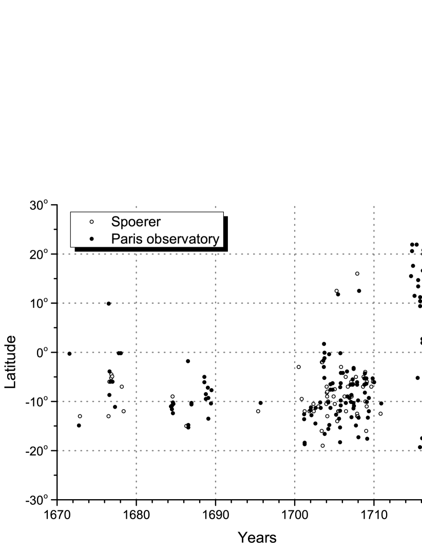
Figure 1: The “Maunder butterflies” for the Spörer catalog [1] (empty circles) and the observations of the Paris observatory[2] (filled circles).

2 Data and method

We used latitudes of sunspots from the paper of Spörer [1] (64 observations) and observations of the Paris observatory (213 observations), which were digitized and compiled to a single catalog in [11]. The “Maunder butterflies” diagram for these catalogs are plotted in Fig. 1. For these data we calculated the “index of sunspot groups” G, which is equal to yearly averaged number of daily observed groups, and yearly dispersions of absolute values of heliographic latitudes of sunspots $\sigma_{\phi}^{2}$.

In these data it is usually unclear whether a single sunspot or a sunspot group was observed, and we will treat all observations as groups. Treating them in opposite way, i.e. as individual sunspot, would affect G but not $\sigma_{\phi}$, and it is the latter values that are of primary importance for us.

We also calculated indices G and $\sigma_{\phi}^{2}$ for the extended Greenwich/NOAA catalog (GC) (1875–2015) [12].

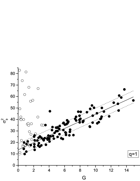
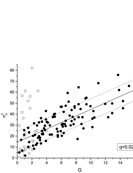
Figure 2: The regressions G — $\sigma_{\phi}^{2}$ (1) for GC: $q=1$ (top) and $q=0.02$ (bottom). The empty circles correspond to years of minimums and adjacent years, which are not taken into account in building of the regressions. The dash lines are for $a+b\,\mbox{G}\pm\Delta$, where $\Delta$ is the rms of regression residuals (2)

In Fig. 2 the dependence G — $\sigma_{\phi}^{2}$ for GC is presented. We do not take into account years of cyclic minimums and adjacent years (the empty circles in Fig. 1), because in that times wings of the “Maunder butterflies” tend to overlap, and, therefore, $\sigma_{\phi}$ can be overestimated. The rest of data (the filled circles) are described well (with the correlation coefficient $r=0.88$) by the linear regression

$$\sigma_{\phi}^{2}=a+b\,\mbox{G}\,,$$ (1)

where $a=13.6\pm 1.0\;{\rm deg}^{2}$ and $b=3.09\pm 0.16\;{\rm deg}^{2}$.

This relation is quite stable to loss of data. For example, if to choose randomly only 2% of sunspot groups observations from GC (hereafter we will refer to the ratio of the number of the residuary observations of sunspot groups to their total number as “the loss ratio” $q$; in this case $q=0.02$), the errors raise, but the coefficients of the regression, within the error limits, do not change: $a=14.5\pm 1.9\;{\rm deg}^{2}$ and $b=2.98\pm 0.26\;{\rm deg}^{2}$ ($r=0.75$) (Fig. 2b). (The dependence of the coefficients on $q$ was in more details discussed in [4].) One can use regression (1) to obtain estimates of G by $\sigma_{\phi}^{2}$. The standard errors of the obtained G can be estimated as $\delta\mbox{G}=\Delta/b$, where

$$\Delta=\sqrt{\frac{1}{N}\sum_{i=1}^{N}\left((\sigma_{\phi}^{2})_{i}-a-b\,\mbox{G}_{i}\right)^{2}}$$ (2)

is the rms of the regression residuals (here the subscripts $i$ is the number of the year for which indices are calculated). Strictly speaking, one should calculate the residuals in (2) for a given interval of G, but they are weakly dependent on G (see Fig. 2) and we can look for the estimate of errors summing over the total set of indices $i$. The dependence of $\delta\mbox{G}$ on the loss ratio $q$ is shown in Fig. 3, where each point for the given $q$ was calculated as a mean of 12 random runs.

Figure 3: The dependence of the standard errors $\delta\mbox{G}$ on the loss ratio $q$ for GC.

Having reconstructed G by known $\sigma_{\phi}$, we can estimate the loss ratio $q$ as $\mbox{G}_{0}/\mbox{G}$, where $\mbox{G}_{0}$ is (generally speaking, underestimated) “index of sunspot groups”, calculated by a fragmentary observational data. After that we can find the error of reconstruction $\delta\mbox{G}$ for the given $q$ using the empirical dependence shown in Fig. 3.

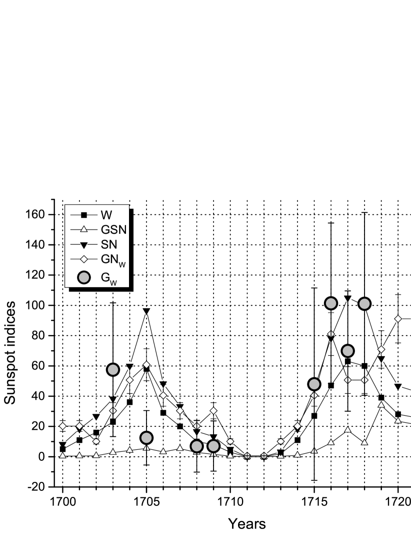
Figure 4: The sunspot indices (scaled to the Wolf number) in the end of the Maunder minimum.

3 Results and discussion

Until the beginning of the 18th century the number of observation in the catalog under investigation is too small to estimate the latitude dispersion correctly. Therefore, we apply the described method to the data starting from 1700. The estimates are made only for years with four or more observations and for the cases when it leads to positive values. Besides, in the first cycle we have taken into account that sunspots existed in the south hemisphere only and the estimate evaluated by the regression must be divided by 2.

We will compare the estimates with other indices of activity known for this epoch: W, GSN and their recently revised versions SN and GN [5, 6, 13]. To make the comparison more transparent it is convenient to renormalize the obtained G, introducing $\mbox{G}_{\mbox{w}}=11.9\,\mbox{G}$, where the coefficient is selected to minimize the rms difference between W and $\mbox{G}_{\mbox{w}}$ for the epoch 1875–1976. The same procedure is made for GN, leading to $\mbox{GN}_{\mbox{w}}=13.2\,\mbox{GN}$.

The correlation coefficient of yearly indices W, $\mbox{G}_{\mbox{w}}$, GSN and $\mbox{GN}_{\mbox{w}}$ for the Greenwich epoch 1875–1976 is higher than 0.98 and their rms difference is less than 10 units. Therefore, for rough estimates of activity in MM we do not make difference between these four indices, expecting them to give approximately the same, by the order of magnitude, level of activity.

In Fig. 4 we compare these indices and our estimates $\mbox{G}_{\mbox{w}}$ for years 1700–1719 (cycles Nos. $-3$ and $-4$ in Wolf’s numeration). Comparison of amplitudes and moments of maxima of cycles is made in Table 1 (the asterisk marks the year of the first of two maximums of $\mbox{GN}_{\mbox{w}}$ in cycle $-3$).

Table 1: Amplitudes and moments (in brackets) of the 11-year cycles of solar activity Nos. $-4$ and $-3$ in different sunspot indices.

No.	Amplitudes of cycles and years of maximums
of cycle	$\mbox{G}_{\mbox{w}}$	W	GSN	SN	$\mbox{GN}_{\mbox{w}}$
$-4$	$58\pm 44$ (1703)	58 (1706)	5.5 (1705)	97 (1705)	$70\pm 12$ (1705)
$-3$	$101\pm 53$ (1716)	63 (1717)	34 (1719)	105 (1717)	$93\pm 16$ (1716)*

One can see that our estimates of amplitudes are, in spite of large uncertainties, in fair agreement with three indices (W, SN, $\mbox{GN}_{\mbox{w}}$) and in significantly less agreement with GSN. The latter index is lower for both cycles and its difference from $\mbox{G}_{\mbox{w}}$ is more than 1.2 standard deviations; it means that $\mbox{G}_{\mbox{w}}>\mbox{GSN}$ with probability about 90%. The moment of the sunspot latitude dispersion maximum in cycle $-3$ also agrees with other data. For cycle $-4$ it is shifted three years to the past, which can be a result of loss of data in years 1704–1706.

Of course, the obtained estimates are correct under assumptions that a) the latitudes of sunspots in the catalogs do not contain systematic errors, and b) the linear regression (1) found for “common” epoch was the same in epochs of grand minimums. Under these assumptions the latitude distribution of sunspots, in agreement with the Wolf number and new revisited indices of activity SN and GN, gives independent evidences in favor of not extremely low cycles $-3$ and $-4$. Thus, the classical Wolf numbers, evidently, describe solar activity in the end of the Maunder minimum more correct than GSN do. The latitudinal data also confirm the conclusion (see [6]) that the MM ended in the very beginning of the 18th century rather than in 1720s.

4 Acknowledgements

The work was supported by the RFBR grant No. 16-02-00090 and the programs of the Presidium of the Russian Academy of Sciences Nos. 21 and 22.

References

- [1] Spörer G, Über die periodicität der Sonnenflecken seit dem Jahr 1618, Nova Acta der Ksl. Leop.-Carol. Deutschen Akademie der Naturforscher, 1889, vol. 53, No. 2, pp. 281–324.
- [2] Ribes J.C. and Nesme-Ribes E., The solar sunspot cycle in the Maunder minimum AD1645 to AD1715, Astron. Astrophys., 1993, vol. 276, pp. 549–563.
- [3] Ivanov V.G., Miletsky E.V., and Nagovitsyn Yu.A., Form of the Latitude Distribution of Sunspot Activity, Astronomy Reports, 2011, vol. 55, No. 10, pp. 911–917.
- [4] Ivanov V.G. and Miletsky E.V., Characteristics of Sunspot Longitudinal Distribution and their Correlation with Solar Activity in Pre-Greenwich Data, Geomagnetism and Aeronomy, 2016, vol. 56, No. 7, pp. 848–852.
- [5] Clette F., Svalgaard L., Vaquero J.M., and Cliver E.W., Revisiting the Sunspot Number. A 400-Year Perspective on the Solar Cycle, Space Science Reviews, 2014, vol. 186, iss. 1–4, pp. 35–103.
- [6] Svalgaard L. and Schatten K.H., Reconstruction of the Sunspot Group Number: The Backbone Method, Sol. Phys., 2016, vol. 291(9), pp. 2653–2684.
- [7] Hoyt D.V. and Schatten K.H., Group sunspot numbers: a new solar activity reconstruction, Solar Phys., 1998, vol. 181(2), pp. 491–512.
- [8] Eddy J.A., The Maunder minimum. Science, 1976, vol. 192, pp. 1189–1202.
- [9] Usoskin I.G. et al. The Maunder minimum (1645–1715) was indeed a grand minimum: A reassessment of multiple datasets, Astron. Astrophys., 2015, vol. 581, p. A95.
- [10] Zolotova N.V. and Ponyavin D.I., How Deep Was the Maunder Minimum? Sol. Phys., 2016, vol. 291(9), pp. 2869–2890.
- [11] Vaquero J.M., Nogales J.M., and Sánchez-Bajo F., Sunspot latitudes during the Maunder Minimum: A machine-readable catalogue from previous studies, Advances in Space Research, 2015, vol. 55(6), pp. 1546–1552.
- [12] http://solarscience.msfc.nasa.gov/greenwch.shtml
- [13] http://www.sidc.be/silso/groupnumber