11institutetext: Department of Applied Mathematics, School of Physical Sciences, Babasaheb Bhimrao Ambedkar University, Lucknow 226025 Uttar Pradesh INDIA 11email: bksingh0584@gmail.com

Algorithms based on DQM with new sets of base functions for solving parabolic partial differential equations in (2+1)21(2+1) dimension

Brajesh Kumar Singh Address for Correspondence: Department of Applied Mathematics, School of Physical Sciences, Babasaheb Bhimrao Ambedkar University, Lucknow 226025 Uttar Pradesh INDIA    Pramod Kumar
Abstract

This paper deals with the numerical computations of two space dimensional time dependent parabolic partial differential equations by adopting adopting an optimal five stage fourth-order strong stability preserving Runge - Kutta (SSP-RK54) scheme for time discretization, and three methods of differential quadrature with different sets of modified B-splines as base functions, for space discretization: namely- i)i) mECDQM: (DQM with modified extended cubic B-splines); ii)ii) mExp-DQM: DQM with modified exponential cubic B-splines, and iii)iii) MTB-DQM: DQM with modified trigonometric cubic B–splines. Specially, we implement these methods on convection-diffusion equation to convert them into a system of first order ordinary differential equations (ODEs), in time. The resulting system of ODEs can be solved using any time integration method, while we prefer SSP-RK54 scheme. All the three methods are found stable for two space convection-diffusion equation by employing matrix stability analysis method. The accuracy and validity of the methods are confirmed by three test problems of two dimensional convection-diffusion equation, which shows that the proposed approximate solutions by any of the method are in good agreement with the exact solutions.

Keywords: Convection-diffusion equation, modified trigonometric cubic-B-splines, modified exponential cubic-B-splines, modified extended cubic-B-splines, differential quadrature method, SSP-RK54 scheme, Thomas algorithm

1 Introduction

The convection-diffusion model can be expressed mathematically, which is a semi linear parabolic partial differential equation. Specially, we consider an initial value system of convection-diffusion equation in 222 dimension as:

utαx2ux2αy2uy2+βxux+βyuy=0,u(x,y,0)=u0(x,y),}inΩ×(0,T],\left.\begin{split}&\frac{\partial u}{\partial t}-\alpha_{x}\frac{\partial^{2}u}{\partial x^{2}}-\alpha_{y}\frac{\partial^{2}u}{\partial y^{2}}+\beta_{x}\frac{\partial u}{\partial x}+\beta_{y}\frac{\partial u}{\partial y}=0,\\ &u(x,y,0)=u^{0}(x,y),\\ \end{split}\right\}in\quad\Omega\times(0,T], (1)

together with the Dirichlet boundary conditions:

u(a,y,t)=f1(y,t),u(b,y,t)=f2(y,t),u(x,c,t)=f3(x,t),u(x,d,t)=f4(x,t),}onΩ×(0,T],\left.\begin{split}&u(a,y,t)=f_{1}(y,t),\quad u(b,y,t)=f_{2}(y,t),\\ &u(x,c,t)=f_{3}(x,t),\quad u(x,d,t)=f_{4}(x,t),\end{split}\right\}on\quad\partial\Omega\times(0,T], (2)

or Neumann boundary conditions:

ux|x=a,y=g1(y,t),ux|x=b,y=g2(y,t),uy|x,y=c=g3(x,t),uy|x,y=d=g4(x,t),}onΩ×(0,T].\left.\begin{split}&\left.\frac{\partial u}{\partial x}\right|_{x=a,y}=g_{1}(y,t),\quad\left.\frac{\partial u}{\partial x}\right|_{x=b,y}=g_{2}(y,t),\\ &\left.\frac{\partial u}{\partial y}\right|_{x,y=c}=g_{3}(x,t),\quad\left.\frac{\partial u}{\partial y}\right|_{x,y=d}=g_{4}(x,t),\end{split}\right\}on\quad\partial\Omega\times(0,T]. (3)

where ΩΩ\partial\Omega is the boundary of computational domain Ω=[a,b]×[c,d]2Ω𝑎𝑏𝑐𝑑superscript2\Omega=[a,b]\times[c,d]\subset\mathbb{R}^{2}, (0,T]0𝑇(0,T] is time interval, and fi,gisubscript𝑓𝑖subscript𝑔𝑖f_{i},g_{i} (i=1,2,3,4)𝑖1234(i=1,2,3,4) and u0subscript𝑢0u_{0} are known smooth functions, and u(x,y,t)𝑢𝑥𝑦𝑡u(x,y,t) denote heat or vorticity. The parameters: βxsubscript𝛽𝑥\beta_{x} and βysubscript𝛽𝑦\beta_{y} are constant convective velocities while the constants αx>0,αy>0formulae-sequencesubscript𝛼𝑥0subscript𝛼𝑦0\alpha_{x}>0,\alpha_{y}>0 are diffusion coefficients in the direction of x𝑥x and y𝑦y, respectively.

The convection-diffusion models have remarkable applications in various branches of science and engineering, for instance, fluid motion, heat transfer, astrophysics, oceanography, meteorology, semiconductors, hydraulics, pollutant and sediment transport, and chemical engineering. Specially, in computational hydraulics and fluid dynamics to model convection-diffusion of quantities such as mass, heat, energy, vorticity [26]. Many researchers have paid their attention to develop some schemes which could produce accurate, stable and efficient solutions behavior of convection-diffusion problems, see [36, 38, 39, 40, 41, 42] and the references therein.

In the last years, the convection-diffusion equation (1) has been solved numerically using various techniques: namely- finite element method [13], Lattice Boltzmann method [9], finite-difference scheme and higher-order compact finite difference schemes [15, 21, 23, 31, 34]. A nine-point high-order compact implicit scheme proposed by Noye and Tan [22] is third-order accurate in space and second-order accurate in time, and has a large zone of stability. An extension of higher order compact difference techniques for steady-state [23] to the time-dependent problems have been presented by Spotz and Carey [29], are fourth-order accurate in space and second or lower order accurate in time but conditionally stable. The fourth-order compact finite difference unconditionally stable scheme due to Dehghan and Mohebbi [12] have the accuracy of order O(h4,t4)𝑂superscript4superscript𝑡4O(h^{4},t^{4}). A family of unconditionally stable finite difference schemes presented in [7] have the accuracy of order O(h3,t2)𝑂superscript3superscript𝑡2O(h^{3},t^{2}). The schemes presented in [17] are based on high-order compact scheme and weighted time discretization, are second or lower order accurate in time and fourth-order accurate in space. The high-order alternating direction implicit (ADI) scheme with accuracy of order O(h4,t2)𝑂superscript4superscript𝑡2O(h^{4},t^{2}) proposed by Karaa and Zhang [18], is unconditionally stable. A high-order unconditionally stable exponential scheme for unsteady 111D convection-diffusion equation by Tian and Yua [32] have the accuracy of order O(h4,t2)𝑂superscript4superscript𝑡2O(h^{4},t^{2}). A rational high-order compact alternating direction implicit (ADI) method have been developed for solving 222D unsteady convection-diffusion problems [30] is unconditionally stable and have the accuracy of order O(h4,t2)𝑂superscript4superscript𝑡2O(h^{4},t^{2}). A unconditionally stable fourth-order compact finite difference approximation for discretizing spatial derivatives and the cubic C1subscript𝐶1C_{1}- spline collocation method in time, proposed by Mohebbi and Dehghan [20], have the accuracy of order O(h4,t4)𝑂superscript4superscript𝑡4O(h^{4},t^{4}). An unconditionally stable, semi-discrete based on Pade approximation, by Ding and Zhang [14], is fourth-order accurate in space and in time both. The most of schemes are based on the two-level finite difference approximations with Dirichlet conditions, and very few schemes have been developed to solve the convection-diffusion equation with Neumann’s boundary conditions, see [6, 33] and references therein. The fourth-order compact finite difference scheme by Cao et al. [6] is of 555th-order accurate in time and 4th-order in the space. A high-order alternating direction implicit scheme based on fourth-order Pade approximation developed by You [33] is unconditionally stable with the accuracy of order O(h4,t2)𝑂superscript4superscript𝑡2O(h^{4},t^{2}).

The differential quadrature method (DQM) dates back to Bellman et al. [5]. After the seminal paper of Bellman, various test functions have been proposed, among others, spline functions, sinc function, Lagrange interpolation polynomials, radial base functions, modified cubic B-splines, see [19, 24, 25, 27, 28, 1, 2, 3, 4], etc. Shu and Richards [27] have generalized approach of DQM for numerical simulation of incompressible Navier-Stokes equation. The main goal of this paper is to find numerical solution of initial value system of 222D convection-diffusion equation with both kinds of boundary conditions (Dirichlet boundary conditions and Neumann boundary conditions), approximated by DQM with new sets of modified cubic B-splines (modified extended cubic B-splines, modified exponential cubic B-splines, modified trigonometric cubic B-splines) as base functions, and so called modified trigonometric cubic-B-spline differential quadrature method (MTB-DQM), modified exponential cubic-B-spline differential quadrature method (mExp-DQM) and third modified extended cubic-B-spline differential quadrature method (mECDQ). These methods are used to transform the convection diffusion problem into a system of first order ODEs, in time. The resulting system of ODEs can be solved by using various time integration algorithm, among them, we prefer SSP-RK54 scheme [45, 46] due to its reduce storage space, which results in less accumulation errors. The accuracy and adaptability of the method is illustrated by three test problems of two dimensional convection diffusion equations.

The rest of the paper is organized into five more sections, which follow this introduction. Specifically, Section 2 deals with the description of the methods: namely- MTB-DQM, mExp-DQM and mECDQ. Section 3 is devoted to the procedure for the implementation of describe above these methods for the system (1) together with the boundary conditions as in (2) and (3). Section 4 deals with the stability analysis of the methods. Section 5 deals with the main goal of the paper is the numerical computation of three test problems. Finally, Section 6 concludes the results.

2 Description of the methods

The differential quadrature method is an approximation to derivatives of a function is the weighted sum of the functional values at certain nodes [5]. The weighting coefficients of the derivatives is depend only on grids [27]. This is the reason for taking the partitions P[Ω]𝑃delimited-[]ΩP[\Omega] of the problem domain Ω={(x,y)R2:0x,y1}Ωconditional-set𝑥𝑦superscript𝑅2formulae-sequence0𝑥𝑦1\Omega=\{(x,y)\in R^{2}:0\leq x,y\leq 1\} distributed uniformly as follows:

P[Ω]={(xi,yj)Ω:hx=xi+1xi,hy=yj+1yj,iΔx,jΔy},𝑃delimited-[]Ωconditional-setsubscript𝑥𝑖subscript𝑦𝑗Ωformulae-sequencesubscript𝑥subscript𝑥𝑖1subscript𝑥𝑖formulae-sequencesubscript𝑦subscript𝑦𝑗1subscript𝑦𝑗formulae-sequence𝑖subscriptΔ𝑥𝑗subscriptΔ𝑦P[\Omega]=\{(x_{i},y_{j})\in\Omega:h_{x}=x_{i+1}-x_{i},h_{y}=y_{j+1}-y_{j},i\in\Delta_{x},j\in\Delta_{y}\},

where Δx={1,2,,Nx},Δy={1,2,,Ny}formulae-sequencesubscriptΔ𝑥12subscript𝑁𝑥subscriptΔ𝑦12subscript𝑁𝑦\Delta_{x}=\{1,2,\ldots,N_{x}\},\Delta_{y}=\{1,2,\ldots,N_{y}\}, and hx=1Nx1 and hy=1Ny1subscript𝑥1subscript𝑁𝑥1 and subscript𝑦1subscript𝑁𝑦1h_{x}=\frac{1}{N_{x}-1}\mbox{ and }h_{y}=\frac{1}{N_{y}-1} are the discretization steps in both x𝑥x and y𝑦y directions, respectively. That is, a uniform partition in each x,y𝑥𝑦x,y-direction with the following grid points:

0=x1<x2<<xi<<xNx1<xNx=1,0subscript𝑥1subscript𝑥2subscript𝑥𝑖subscript𝑥subscript𝑁𝑥1subscript𝑥subscript𝑁𝑥10=x_{1}<x_{2}<\ldots<x_{i}<\ldots<x_{N_{x}-1}<x_{N_{x}}=1,
0=y1<y2<<yj<<yNy1<yNy=1.0subscript𝑦1subscript𝑦2subscript𝑦𝑗subscript𝑦subscript𝑁𝑦1subscript𝑦subscript𝑁𝑦10=y_{1}<y_{2}<\ldots<y_{j}<\ldots<y_{N_{y}-1}<y_{N_{y}}=1.

Let (xi,yj)subscript𝑥𝑖subscript𝑦𝑗(x_{i},y_{j}) be the generic grid point and

uijuij(t)u(xi,yj,t),iΔx,jΔy.formulae-sequencesubscript𝑢𝑖𝑗subscript𝑢𝑖𝑗𝑡𝑢subscript𝑥𝑖subscript𝑦𝑗𝑡formulae-sequence𝑖subscriptΔ𝑥𝑗subscriptΔ𝑦u_{ij}\equiv u_{ij}(t)\equiv u(x_{i},y_{j},t),~{}~{}i\in\Delta_{x},j\in\Delta_{y}.

The r𝑟r-th order derivative of u(x,y,t)𝑢𝑥𝑦𝑡u(x,y,t), for r{1,2}𝑟12r\in\{1,2\}, with respect to x,y𝑥𝑦x,y at (xi,yj)subscript𝑥𝑖subscript𝑦𝑗(x_{i},y_{j}) for iΔx,jΔyformulae-sequence𝑖subscriptΔ𝑥𝑗subscriptΔ𝑦i\in\Delta_{x},j\in\Delta_{y} is approximated as follows:

ruxr)ij==1Nxai(r)uj,iΔx,i=1,2,Nruyr)ij==1Nybj(r)ui,jΔy,i=1,2,M\begin{split}&\left.\frac{\partial^{r}u}{\partial x^{r}}\right)_{ij}=\sum_{\ell=1}^{N_{x}}a_{i\ell}^{(r)}u_{\ell j},\qquad i\in\Delta_{x},\quad i=1,2,\ldots N\\ &\left.\frac{\partial^{r}u}{\partial y^{r}}\right)_{ij}=\sum_{\ell=1}^{N_{y}}b_{j\ell}^{(r)}u_{i\ell},\qquad j\in\Delta_{y},\quad i=1,2,\ldots M\end{split} (4)

where the coefficients aip(r)superscriptsubscript𝑎𝑖𝑝𝑟a_{ip}^{(r)} and bjp(r)superscriptsubscript𝑏𝑗𝑝𝑟b_{jp}^{(r)}, the time dependent unknown quantities, are termed as the weighting functions of the r𝑟rth-order derivative, to be computed using various type of base functions.

2.1 The MTB-DQM

The trigonometric cubic B-spline function Ti=Ti(x)subscript𝑇𝑖subscript𝑇𝑖𝑥T_{i}=T_{i}(x) at node i𝑖i in x𝑥x direction, read as [35, 43]:

Ti=1ω{p3(xi),x[xi,xi+1)p(xi){p(xi)q(xi+2)+p(xi+1)q(xi+3)}+p2(xi+1)q(xi+4),x[xi+1,xi+2)q(xi+4){p(xi+1q(xi+3)+p(xi+2)q(xi+4)}+p(xi)q2(xi+3),x[xi+2,xi+3)q3(xi+4),x[xi+3,xi+4)\displaystyle T_{i}=\frac{1}{\omega}\left\{\begin{array}[]{ll}p^{3}(x_{i}),&x\in[x_{i},x_{i+1})\\ p(x_{i})\{p(x_{i})q(x_{i+2})+p(x_{i+1})q(x_{i+3})\}+p^{2}(x_{i+1})q(x_{i+4}),&x\in[x_{i+1},x_{i+2})\\ q(x_{i+4})\{p(x_{i+1}q(x_{i+3})+p(x_{i+2})q(x_{i+4})\}+p(x_{i})q^{2}(x_{i+3}),&x\in[x_{i+2},x_{i+3})\\ q^{3}(x_{i+4}),&x\in[x_{i+3},x_{i+4})\end{array}\right. (9)

where p(xi)=sin(xxi2);q(xi)=sin(xix2)formulae-sequence𝑝subscript𝑥𝑖𝑥subscript𝑥𝑖2𝑞subscript𝑥𝑖subscript𝑥𝑖𝑥2p(x_{i})=\sin(\frac{x-x_{i}}{2});~{}~{}q(x_{i})=\sin(\frac{x_{i}-x}{2}), ω=sin(hx2)sin(hx)sin(3hx2)𝜔subscript𝑥2subscript𝑥3subscript𝑥2\omega=\sin\left(\frac{h_{x}}{2}\right)\sin\left(h_{x}\right)\sin\left(\frac{3h_{x}}{2}\right). Then the set {T0,,TNx,TNx+1}subscript𝑇0subscript𝑇subscript𝑁𝑥subscript𝑇subscript𝑁𝑥1\{T_{0},\ldots,T_{N_{x}},T_{N_{x}+1}\} forms a base over the interval [a,b]𝑎𝑏[a,b]. Setting

a1=sin2(hx2)sin(hx)sin(3hx2);a2=21+2cos(hx);a4=34sin(3hx2)=a3;a5=3+9cos(hx)16sin2(hx2)(2cos(hx2)+cos(3hx2));a6=3cos2(hx2)sin2(hx2)(2+4cos(hx)).\begin{split}&a_{1}=\frac{\sin^{2}\left(\frac{h_{x}}{2}\right)}{\sin(h_{x})\sin\left(\frac{3h_{x}}{2}\right)};\quad a_{2}=\frac{2}{1+2\cos(h_{x})};\quad a_{4}=\frac{3}{4\sin\left(\frac{3h_{x}}{2}\right)}=-a_{3};\\ &a_{5}=\frac{3+9\cos(h_{x})}{16\sin^{2}\left(\frac{h_{x}}{2}\right)\left(2\cos\left(\frac{h_{x}}{2}\right)+\cos\left(\frac{3h_{x}}{2}\right)\right)};\quad a_{6}=\frac{3\cos^{2}(\frac{h_{x}}{2})}{\sin^{2}\left(\frac{h_{x}}{2}\right)\left(2+4\cos\left(h_{x}\right)\right)}.\end{split}

The values of Tisubscript𝑇𝑖T_{i} and its first and second derivatives in the grid point xjsubscript𝑥𝑗x_{j}, denoted by Tij:=Ti(xj)assignsubscript𝑇𝑖𝑗subscript𝑇𝑖subscript𝑥𝑗T_{ij}:=T_{i}(x_{j}), Tij:=Ti(xj)assignsubscriptsuperscript𝑇𝑖𝑗subscriptsuperscript𝑇𝑖subscript𝑥𝑗T^{\prime}_{ij}:=T^{\prime}_{i}(x_{j}) and Tij′′:=Ti′′(xj)assignsubscriptsuperscript𝑇′′𝑖𝑗subscriptsuperscript𝑇′′𝑖subscript𝑥𝑗T^{\prime\prime}_{ij}:=T^{\prime\prime}_{i}(x_{j}), respectively, read:

Tij={a2, if ij=0a1, if ij=±10,otherwise;Tij={a4, if ij=1a3, if ij=10,otherwise; Tij′′={a6, if ij=0a5, if ij=±10otherwiseformulae-sequencesubscript𝑇𝑖𝑗casessubscript𝑎2 if 𝑖𝑗0subscript𝑎1 if 𝑖𝑗plus-or-minus10otherwiseformulae-sequencesubscriptsuperscript𝑇𝑖𝑗casessubscript𝑎4 if 𝑖𝑗1subscript𝑎3 if 𝑖𝑗10otherwise subscriptsuperscript𝑇′′𝑖𝑗casessubscript𝑎6 if 𝑖𝑗0subscript𝑎5 if 𝑖𝑗plus-or-minus10otherwise\displaystyle T_{ij}=\left\{\begin{array}[]{ll}a_{2},&\mbox{ if }i-j=0\\ a_{1},&\mbox{ if }i-j=\pm 1\\ 0,&\mbox{otherwise}\end{array}\right.;\quad T^{\prime}_{ij}=\left\{\begin{array}[]{ll}a_{4},&\mbox{ if }i-j=1\\ a_{3},&\mbox{ if }i-j=-1\\ 0,&\mbox{otherwise}\end{array}\right.;\mbox{\quad}T^{\prime\prime}_{ij}=\left\{\begin{array}[]{ll}a_{6},&\mbox{ if }i-j=0\\ a_{5},&\mbox{ if }i-j=\pm 1\\ 0&\mbox{otherwise}\end{array}\right. (19)

The modified trigonometric cubic B-splines base functions are defined as follows [1, 4]:

{τ1(x)=T1(x)+2T0(x)τ2(x)=T2(x)T0(x)τj(x)=Tj(x), for j=3,4,,Nx2τNx1(x)=TNx1(x)TNx+1(x)τNx(x)=TNx(x)+2TNx+1(x)\left\{\begin{split}&\tau_{1}(x)=T_{1}(x)+2T_{0}(x)\\ &\tau_{2}(x)=T_{2}(x)-T_{0}(x)\\ &\vdots\\ &\tau_{j}(x)=T_{j}(x),\mbox{ for }j=3,4,\ldots,N_{x}-2\\ &\vdots\\ &\tau_{N_{x}-1}(x)=T_{N_{x}-1}(x)-T_{N_{x}+1}(x)\\ &\tau_{N_{x}}(x)=T_{N_{x}}(x)+2T_{N_{x}+1}(x)\end{split}\right. (20)

Now, the set {τ1,τ2,,τNx}subscript𝜏1subscript𝜏2subscript𝜏subscript𝑁𝑥\{\tau_{1},\tau_{2},\ldots,\tau_{N_{x}}\} is the base over [a,b]𝑎𝑏[a,b]. The procedure to define modified trigonometric cubic B-splines in y𝑦y direction, is followed analogously.

2.1.1 The evaluation of the weighting coefficients aij(r)superscriptsubscript𝑎𝑖𝑗𝑟a_{ij}^{(r)} and bij(r)(r=1,2)superscriptsubscript𝑏𝑖𝑗𝑟𝑟12b_{ij}^{(r)}(r=1,2)

In order to evaluate the weighting coefficients aip(1)superscriptsubscript𝑎𝑖𝑝1a_{ip}^{(1)} of first order partial derivative in Eq. (4), we use the modified trigonometric cubic B-spline τp(x)subscript𝜏𝑝𝑥\tau_{p}(x), pΔx𝑝subscriptΔ𝑥p\in\Delta_{x} in DQ method as base functions. Setting τpi:=τp(xi)assignsubscriptsuperscript𝜏𝑝𝑖superscriptsubscript𝜏𝑝subscript𝑥𝑖\tau^{\prime}_{pi}:=\tau_{p}^{\prime}(x_{i}) and τp:=τp(x)assignsubscript𝜏𝑝subscript𝜏𝑝subscript𝑥\tau_{p\ell}:=\tau_{p}(x_{\ell}). Using MTB-DQM, the approximate values of first order derivative is obtained as follows:

τpi==1Nxai(1)τp,p,iΔx.formulae-sequencesubscriptsuperscript𝜏𝑝𝑖superscriptsubscript1subscript𝑁𝑥superscriptsubscript𝑎𝑖1subscript𝜏𝑝𝑝𝑖subscriptΔ𝑥\tau^{\prime}_{pi}=\sum_{\ell=1}^{N_{x}}a_{i\ell}^{(1)}\tau_{p\ell},\qquad p,i\in\Delta_{x}. (21)

Setting =[τp]delimited-[]subscript𝜏𝑝\Im=[\tau_{p\ell}], A=[ai(1)]𝐴delimited-[]superscriptsubscript𝑎𝑖1A=[a_{i\ell}^{(1)}], and =[τp]superscriptdelimited-[]subscriptsuperscript𝜏𝑝\Im^{\prime}=[\tau^{\prime}_{p\ell}]. Eq. (21) reduced to compact matrix form:

AT=.superscript𝐴𝑇superscript\Im A^{T}=\Im^{\prime}. (22)

The coefficient matrix \Im of order Nxsubscript𝑁𝑥N_{x} can be read from (19) and (20) as:

=[a2+2a1 a1     a2 a1     a1 a2 a1            a1 a2 a1     a1 a2 0     a1 a2+2a1]delimited-[]subscript𝑎22subscript𝑎1 subscript𝑎1     missing-subexpressionmissing-subexpressionsubscript𝑎2 subscript𝑎1    missing-subexpressionmissing-subexpression subscript𝑎1 subscript𝑎2 subscript𝑎1   missing-subexpressionmissing-subexpression      missing-subexpressionmissing-subexpression   subscript𝑎1 subscript𝑎2 subscript𝑎1 missing-subexpressionmissing-subexpression    subscript𝑎1 subscript𝑎2 0missing-subexpression     subscript𝑎1 subscript𝑎22subscript𝑎1missing-subexpression\Im=\left[\begin{array}[]{cccccccc}a_{2}+2a_{1}$\quad$&a_{1}$\quad$&$\quad$&$\quad$&$\quad$&$\quad$&\\ $0 \quad$&a_{2}$\quad$&a_{1}$\quad$&$\quad$&$\quad$&$\quad$&\\ $\quad$&a_{1}$\quad$&a_{2}$\quad$&a_{1}$\quad$&$\quad$&$\quad$&\\ $\quad$&$\quad$&\ddots$\quad$&\ddots$\quad$&\ddots$\quad$&$\quad$&\\ $\quad$&$\quad$&$\quad$&a_{1}$\quad$&a_{2}$\quad$&a_{1}$\quad$&\\ $\quad$&$\quad$&$\quad$&$\quad$&a_{1}$\quad$&a_{2}$\quad$&$0$\\ $\quad$&$\quad$&$\quad$&$\quad$&$\quad$&a_{1}$\quad$&a_{2}+2a_{1}\\ \end{array}\right]

and the columns of the matrix superscript\Im^{\prime} read as:

[1]=[2a4a3a4000],[2]=[a40a300],,[Nx1]=[00a40a3], and [Nx]=[002a4a3a4].formulae-sequencesuperscript1delimited-[]2subscript𝑎4subscript𝑎3subscript𝑎40missing-subexpression00formulae-sequencesuperscript2delimited-[]subscript𝑎40subscript𝑎30missing-subexpression0formulae-sequencesuperscriptsubscript𝑁𝑥1delimited-[]0missing-subexpression0subscript𝑎40subscript𝑎3 and superscriptsubscript𝑁𝑥delimited-[]0missing-subexpressionmissing-subexpression02subscript𝑎4subscript𝑎3subscript𝑎4\Im^{\prime}[1]=\left[\begin{array}[]{c}2a_{4}\\ a_{3}-a_{4}\\ 0\\ \vdots\\ \\ 0\\ 0\\ \end{array}\right],\Im^{\prime}[2]=\left[\begin{array}[]{c}a_{4}\\ $0$\\ a_{3}\\ $0$\\ \vdots\\ \\ $0$\\ \end{array}\right],\ldots,\Im^{\prime}[N_{x}-1]=\left[\begin{array}[]{c}$0$\\ \vdots\\ \\ $0$\\ a_{4}\\ $0$\\ a_{3}\\ \end{array}\right],\mbox{ and }\Im^{\prime}[N_{x}]=\left[\begin{array}[]{c}$0$\\ \\ \vdots\\ \\ $0$\\ 2a_{4}\\ a_{3}-a_{4}\\ \end{array}\right].

2.2 The mExp-DQM

The exponential cubic B-splines function ζi=ζi(x)subscript𝜁𝑖subscript𝜁𝑖𝑥\zeta_{i}=\zeta_{i}(x) at node i𝑖i in x𝑥x direction, reads [40, 41]:

ζi=1hx3{b2{(xi2x)1psinh(p(xi2x))},x[xi2,xi1)a1+b1(xix)+c1exp(p(xix))+d1exp(p(xix)),x[xi1,xi)a1+b1(xxi)+c1exp(p(xxi))+d1exp(p(xxi)),x[xi,xi+1)b2{(xxi+2)1psinh(p(xxi+2))},x[xi+1,xi+2)0,otherwisesubscript𝜁𝑖1superscriptsubscript𝑥3casessubscript𝑏2subscript𝑥𝑖2𝑥1𝑝𝑝subscript𝑥𝑖2𝑥𝑥subscript𝑥𝑖2subscript𝑥𝑖1subscript𝑎1subscript𝑏1subscript𝑥𝑖𝑥subscript𝑐1𝑝subscript𝑥𝑖𝑥subscript𝑑1𝑝subscript𝑥𝑖𝑥𝑥subscript𝑥𝑖1subscript𝑥𝑖subscript𝑎1subscript𝑏1𝑥subscript𝑥𝑖subscript𝑐1𝑝𝑥subscript𝑥𝑖subscript𝑑1𝑝𝑥subscript𝑥𝑖𝑥subscript𝑥𝑖subscript𝑥𝑖1subscript𝑏2𝑥subscript𝑥𝑖21𝑝𝑝𝑥subscript𝑥𝑖2𝑥subscript𝑥𝑖1subscript𝑥𝑖20otherwise\displaystyle\zeta_{i}=\frac{1}{h_{x}^{3}}\left\{\begin{array}[]{ll}b_{2}\{(x_{i-2}-x)-\frac{1}{p}\sinh(p(x_{i-2}-x))\},&x\in[x_{i-2},x_{i-1})\\ a_{1}+b_{1}(x_{i}-x)+c_{1}\exp(p(x_{i}-x))+d_{1}\exp(p(x_{i}-x)),&x\in[x_{i-1},x_{i})\\ a_{1}+b_{1}(x-x_{i})+c_{1}\exp(p(x-x_{i}))+d_{1}\exp(p(x-x_{i})),&x\in[x_{i},x_{i+1})\\ b_{2}\{(x-x_{i+2})-\frac{1}{p}\sinh(p(x-x_{i+2}))\},&x\in[x_{i+1},x_{i+2})\\ 0,&\mbox{otherwise}\end{array}\right. (28)

where

a1=pchxpchxs;b1=p2(s2c(1c)(pchxs)(1c)),b2=p2(pchxs),c=cosh(phx),s=sinh(phx),c1=14{exp(phx)(1c)+s(exp(phx)1)(pchxs)(1c)},d1=14{exp(phx)(c1)+s(exp(phx)1)(pchxs)(1c)}.formulae-sequencesubscript𝑎1𝑝𝑐subscript𝑥𝑝𝑐subscript𝑥𝑠formulae-sequencesubscript𝑏1𝑝2superscript𝑠2𝑐1𝑐𝑝𝑐subscript𝑥𝑠1𝑐formulae-sequencesubscript𝑏2𝑝2𝑝𝑐subscript𝑥𝑠formulae-sequence𝑐𝑝subscript𝑥formulae-sequence𝑠𝑝subscript𝑥formulae-sequencesubscript𝑐114𝑝subscript𝑥1𝑐𝑠𝑝subscript𝑥1𝑝𝑐subscript𝑥𝑠1𝑐subscript𝑑114𝑝subscript𝑥𝑐1𝑠𝑝subscript𝑥1𝑝𝑐subscript𝑥𝑠1𝑐\begin{split}&a_{1}=\frac{pch_{x}}{pch_{x}-s};b_{1}=\frac{p}{2}\left(\frac{s^{2}-c(1-c)}{(pch_{x}-s)(1-c)}\right),b_{2}=\frac{p}{2(pch_{x}-s)},c=\cosh(ph_{x}),s=\sinh(ph_{x}),\\ &c_{1}=\frac{1}{4}\left\{\frac{\exp(-ph_{x})(1-c)+s(\exp(-ph_{x})-1)}{(pch_{x}-s)(1-c)}\right\},d_{1}=\frac{1}{4}\left\{\frac{\exp(ph_{x})(c-1)+s(\exp(ph_{x})-1)}{(pch_{x}-s)(1-c)}\right\}.\end{split}

The set {ζ0,ζ1,ζ2,,ζNx,ζNx+1}subscript𝜁0subscript𝜁1subscript𝜁2subscript𝜁subscript𝑁𝑥subscript𝜁subscript𝑁𝑥1\{\zeta_{0},\zeta_{1},\zeta_{2},\ldots,\zeta_{N_{x}},\zeta_{N_{x}+1}\} forms a base over [a,b]𝑎𝑏[a,b]. Setting the values of ζisubscript𝜁𝑖\zeta_{i} and its first and second derivatives at xjsubscript𝑥𝑗x_{j} by ζij:=ζi(xj)assignsubscript𝜁𝑖𝑗subscript𝜁𝑖subscript𝑥𝑗\zeta_{ij}:=\zeta_{i}(x_{j}), ζij:=ζi(xj)assignsubscriptsuperscript𝜁𝑖𝑗subscriptsuperscript𝜁𝑖subscript𝑥𝑗\zeta^{\prime}_{ij}:=\zeta^{\prime}_{i}(x_{j}) and ζij′′:=ζi′′(xj)assignsubscriptsuperscript𝜁′′𝑖𝑗subscriptsuperscript𝜁′′𝑖subscript𝑥𝑗\zeta^{\prime\prime}_{ij}:=\zeta^{\prime\prime}_{i}(x_{j}), respectively. Then

ζij={1, if ij=0sph2(pchxs), if ij=±10,otherwise;ζij={p(1c)2(pchxs), if ij=1p(1c)2(pchxs), if ij=10,otherwise;ζij={p2s(pchxs), if ij=0p2s2(pchxs), if ij=±10otherwiseformulae-sequencesubscript𝜁𝑖𝑗cases1 if 𝑖𝑗0𝑠𝑝2𝑝𝑐subscript𝑥𝑠 if 𝑖𝑗plus-or-minus10otherwiseformulae-sequencesubscript𝜁𝑖𝑗cases𝑝1𝑐2𝑝𝑐subscript𝑥𝑠 if 𝑖𝑗1𝑝1𝑐2𝑝𝑐subscript𝑥𝑠 if 𝑖𝑗10otherwisesubscript𝜁𝑖𝑗casessuperscript𝑝2𝑠𝑝𝑐subscript𝑥𝑠 if 𝑖𝑗0superscript𝑝2𝑠2𝑝𝑐subscript𝑥𝑠 if 𝑖𝑗plus-or-minus10otherwise\displaystyle\zeta_{ij}=\left\{\begin{array}[]{ll}1,&\mbox{ if }i-j=0\\ \frac{s-ph}{2(pch_{x}-s)},&\mbox{ if }i-j=\pm 1\\ 0,&\mbox{otherwise}\end{array}\right.;~{}~{}\zeta_{ij}=\left\{\begin{array}[]{ll}-\frac{p(1-c)}{2(pch_{x}-s)},&\mbox{ if }i-j=1\\ \frac{p(1-c)}{2(pch_{x}-s)},&\mbox{ if }i-j=-1\\ 0,&\mbox{otherwise}\end{array}\right.;~{}~{}\zeta_{ij}=\left\{\begin{array}[]{ll}-\frac{p^{2}s}{(pch_{x}-s)},&\mbox{ if }i-j=0\\ \frac{p^{2}s}{2(pch_{x}-s)},&\mbox{ if }i-j=\pm 1\\ 0&\mbox{otherwise}\end{array}\right. (38)

The modified exponential cubic B-splines base functions are read as:

{ς1(x)=ζ1(x)+2ζ0(x)ς2(x)=ζ2(x)ζ0(x)ςj(x)=ζj(x), for j=3,4,,Nx2ςNx1(x)=ζNx1(x)ζNx+1(x)ςNx(x)=ζNx(x)+2ζNx+1(x)\left\{\begin{split}&\varsigma_{1}(x)=\zeta_{1}(x)+2\zeta_{0}(x)\\ &\varsigma_{2}(x)=\zeta_{2}(x)-\zeta_{0}(x)\\ &\vdots\\ &\varsigma_{j}(x)=\zeta_{j}(x),\mbox{ for }j=3,4,\ldots,N_{x}-2\\ &\vdots\\ &\varsigma_{N_{x}-1}(x)=\zeta_{N_{x}-1}(x)-\zeta_{N_{x}+1}(x)\\ &\varsigma_{N_{x}}(x)=\zeta_{N_{x}}(x)+2\zeta_{N_{x}+1}(x)\end{split}\right. (39)

The set {ς1,ς2,,ςNx}subscript𝜍1subscript𝜍2subscript𝜍subscript𝑁𝑥\{\varsigma_{1},\varsigma_{2},\ldots,\varsigma_{N_{x}}\} is a base over [a,b]𝑎𝑏[a,b]. The procedure to define modified trigonometric cubic B-splines in y𝑦y direction, is followed analogously.

2.2.1 The evaluation of the weighting coefficients aij(r)superscriptsubscript𝑎𝑖𝑗𝑟a_{ij}^{(r)} and bij(r)(r=1,2)superscriptsubscript𝑏𝑖𝑗𝑟𝑟12b_{ij}^{(r)}(r=1,2)

Setting ςpi:=ςp(xi)assignsubscriptsuperscript𝜍𝑝𝑖superscriptsubscript𝜍𝑝subscript𝑥𝑖\varsigma^{\prime}_{pi}:=\varsigma_{p}^{\prime}(x_{i}) and ςp:=ςp(x)assignsubscript𝜍𝑝subscript𝜍𝑝subscript𝑥\varsigma_{p\ell}:=\varsigma_{p}(x_{\ell}) for all p,Δx𝑝subscriptΔ𝑥p,\ell\Delta_{x}. Using mExp-DQM, the approximate values of the first-order derivative is given by

ςpi==1Nxai(1)ςp,p,iΔx.formulae-sequencesubscriptsuperscript𝜍𝑝𝑖superscriptsubscript1subscript𝑁𝑥superscriptsubscript𝑎𝑖1subscript𝜍𝑝𝑝𝑖subscriptΔ𝑥\varsigma^{\prime}_{pi}=\sum_{\ell=1}^{N_{x}}a_{i\ell}^{(1)}\varsigma_{p\ell},\qquad p,i\in\Delta_{x}. (40)

Setting =[ςp]delimited-[]subscript𝜍𝑝\beth=[\varsigma_{p\ell}], A=[ai(1)]𝐴delimited-[]superscriptsubscript𝑎𝑖1A=[a_{i\ell}^{(1)}], and =[ςp]superscriptdelimited-[]subscriptsuperscript𝜍𝑝\beth^{\prime}=[\varsigma^{\prime}_{p\ell}], then Eq. (40) can be reduced to compact matrix form:

AT=.superscript𝐴𝑇superscript\beth A^{T}=\beth^{\prime}. (41)

Let ω=p(1c)hxpchxs𝜔𝑝1𝑐subscript𝑥𝑝𝑐subscript𝑥𝑠\omega=\frac{p(1-c)h_{x}}{pch_{x}-s} and θ=sphx2(pchxs)𝜃𝑠𝑝subscript𝑥2𝑝𝑐subscript𝑥𝑠\theta=\frac{s-ph_{x}}{2(pch_{x}-s)}. Using Eqns. (38) and (39), the coefficient matrix \beth of order Nxsubscript𝑁𝑥N_{x}, read as:

=[ω θ     1 θ     θ 1 θ            θ 1 θ     θ 1 0     θ ω]delimited-[]𝜔 𝜃     missing-subexpressionmissing-subexpression1 𝜃    missing-subexpressionmissing-subexpression 𝜃 1 𝜃   missing-subexpressionmissing-subexpression      missing-subexpressionmissing-subexpression   𝜃 1 𝜃 missing-subexpressionmissing-subexpression    𝜃 1 0missing-subexpression     𝜃 𝜔missing-subexpression\beth=\left[\begin{array}[]{cccccccc}\omega$\quad$&\theta$\quad$&$\quad$&$\quad$&$\quad$&$\quad$&\\ $0 \quad$&1$\quad$&\theta$\quad$&$\quad$&$\quad$&$\quad$&\\ $\quad$&\theta$\quad$&1$\quad$&\theta$\quad$&$\quad$&$\quad$&\\ $\quad$&$\quad$&\ddots$\quad$&\ddots$\quad$&\ddots$\quad$&$\quad$&\\ $\quad$&$\quad$&$\quad$&\theta$\quad$&1$\quad$&\theta$\quad$&\\ $\quad$&$\quad$&$\quad$&$\quad$&\theta$\quad$&1$\quad$&$0$\\ $\quad$&$\quad$&$\quad$&$\quad$&$\quad$&\theta$\quad$&\omega\\ \end{array}\right]

and the columns of the matrix superscript\beth^{\prime} read:

[1]=[ω/hxω/hx000],[2]=[ω/2hx0ω/2hx00],,[Nx1]=[00ω/2hx0ω/2hx], and [Nx]=[00ω/hxω/hx].formulae-sequencesuperscriptdelimited-[]1delimited-[]𝜔subscript𝑥𝜔subscript𝑥0missing-subexpression00formulae-sequencesuperscriptdelimited-[]2delimited-[]𝜔2subscript𝑥0𝜔2subscript𝑥0missing-subexpression0formulae-sequencesuperscriptdelimited-[]subscript𝑁𝑥1delimited-[]0missing-subexpression0𝜔2subscript𝑥0𝜔2subscript𝑥 and superscriptdelimited-[]subscript𝑁𝑥delimited-[]0missing-subexpressionmissing-subexpression0𝜔subscript𝑥𝜔subscript𝑥\beth^{\prime}[1]=\left[\begin{array}[]{c}\omega/h_{x}\\ -\omega/h_{x}\\ 0\\ \vdots\\ \\ 0\\ 0\\ \end{array}\right],\beth^{\prime}[2]=\left[\begin{array}[]{c}\omega/2h_{x}\\ $0$\\ -\omega/2h_{x}\\ $0$\\ \vdots\\ \\ $0$\\ \end{array}\right],\ldots,\beth^{\prime}[N_{x}-1]=\left[\begin{array}[]{c}$0$\\ \vdots\\ \\ $0$\\ \omega/2h_{x}\\ $0$\\ -\omega/2h_{x}\\ \end{array}\right],\mbox{ and }\beth^{\prime}[N_{x}]=\left[\begin{array}[]{c}$0$\\ \\ \vdots\\ \\ $0$\\ \omega/h_{x}\\ -\omega/h_{x}\\ \end{array}\right].

2.3 The mECDQ method

The extended cubic B-splines function φi=φi(x)subscript𝜑𝑖subscript𝜑𝑖𝑥\varphi_{i}=\varphi_{i}(x), in the x𝑥x direction and at the knots, reads [42, 36, 37]:

φi=124{4(1λ)Pi23(x)+3λPi24(x),x[xi2,xi1)24p+12Pi1(x)+6(2+λ)Pi12(x)12Pi13(x)3λPi14(x),x[xi1,xi)24p12Pi+1(x)+6(2+λ)Pi+12(x)+12Pi+13(x)3λPi+14(x),x[xi,xi+1)4(λ1)Pi+23(x)+3λPi+24(x),x[xi+1,xi+2)0,otherwisesubscript𝜑𝑖124cases41𝜆superscriptsubscript𝑃𝑖23𝑥3𝜆superscriptsubscript𝑃𝑖24𝑥𝑥subscript𝑥𝑖2subscript𝑥𝑖124𝑝12subscript𝑃𝑖1𝑥62𝜆superscriptsubscript𝑃𝑖12𝑥12superscriptsubscript𝑃𝑖13𝑥3𝜆superscriptsubscript𝑃𝑖14𝑥𝑥subscript𝑥𝑖1subscript𝑥𝑖24𝑝12subscript𝑃𝑖1𝑥62𝜆superscriptsubscript𝑃𝑖12𝑥12superscriptsubscript𝑃𝑖13𝑥3𝜆superscriptsubscript𝑃𝑖14𝑥𝑥subscript𝑥𝑖subscript𝑥𝑖14𝜆1superscriptsubscript𝑃𝑖23𝑥3𝜆superscriptsubscript𝑃𝑖24𝑥𝑥subscript𝑥𝑖1subscript𝑥𝑖20otherwise\displaystyle\varphi_{i}=\frac{1}{24}\left\{\begin{array}[]{ll}4(1-\lambda)P_{i-2}^{3}(x)+3\lambda P_{i-2}^{4}(x),&x\in[x_{i-2},x_{i-1})\\ 24p+12P_{i-1}(x)+6(2+\lambda)P_{i-1}^{2}(x)-12P_{i-1}^{3}(x)-3\lambda P_{i-1}^{4}(x),&x\in[x_{i-1},x_{i})\\ 24p-12P_{i+1}(x)+6(2+\lambda)P_{i+1}^{2}(x)+12P_{i+1}^{3}(x)-3\lambda P_{i+1}^{4}(x),&x\in[x_{i},x_{i+1})\\ 4(\lambda-1)P_{i+2}^{3}(x)+3\lambda P_{i+2}^{4}(x),&x\in[x_{i+1},x_{i+2})\\ 0,&\mbox{otherwise}\end{array}\right. (47)

where hxPi(x)=(xxi)subscript𝑥subscript𝑃𝑖𝑥𝑥subscript𝑥𝑖h_{x}P_{i}(x)=(x-x_{i}) and 24=4λ24Weierstrass-p4𝜆24\wp=4-\lambda, and λ𝜆\lambda is a free parameter [36]. The set {φ0,φ1,φ2,,φNx,φNx+1}subscript𝜑0subscript𝜑1subscript𝜑2subscript𝜑subscript𝑁𝑥subscript𝜑subscript𝑁𝑥1\{\varphi_{0},\varphi_{1},\varphi_{2},\ldots,\varphi_{N_{x}},\varphi_{N_{x}+1}\} forms a base over [a,b]𝑎𝑏[a,b]. Let 12hxθ=8+λ12subscript𝑥𝜃8𝜆12h_{x}\theta=8+\lambda and 2hx2ω=2+λ2superscriptsubscript𝑥2𝜔2𝜆2h_{x}^{2}\omega=2+\lambda, then the values of φisubscript𝜑𝑖\varphi_{i} and its first and second derivatives in the grid point xjsubscript𝑥𝑗x_{j}, denoted by φij:=φi(xj)assignsubscript𝜑𝑖𝑗subscript𝜑𝑖subscript𝑥𝑗\varphi_{ij}:=\varphi_{i}(x_{j}), φij:=φi(xj)assignsubscriptsuperscript𝜑𝑖𝑗subscriptsuperscript𝜑𝑖subscript𝑥𝑗\varphi^{\prime}_{ij}:=\varphi^{\prime}_{i}(x_{j}) and φij′′:=φi′′(xj)assignsubscriptsuperscript𝜑′′𝑖𝑗subscriptsuperscript𝜑′′𝑖subscript𝑥𝑗\varphi^{\prime\prime}_{ij}:=\varphi^{\prime\prime}_{i}(x_{j}), respectively, read:

φij={θ, if ij=0, if ij=±10,otherwise;2hxφij={1, if ij=11, if ij=10,otherwise; φij′′={2ω, if ij=0ω, if ij=±10otherwiseformulae-sequencesubscript𝜑𝑖𝑗cases𝜃 if 𝑖𝑗0Weierstrass-p if 𝑖𝑗plus-or-minus10otherwiseformulae-sequence2subscript𝑥subscriptsuperscript𝜑𝑖𝑗cases1 if 𝑖𝑗11 if 𝑖𝑗10otherwise subscriptsuperscript𝜑′′𝑖𝑗cases2𝜔 if 𝑖𝑗0𝜔 if 𝑖𝑗plus-or-minus10otherwise\displaystyle\varphi_{ij}=\left\{\begin{array}[]{ll}\theta,&\mbox{ if }i-j=0\\ \wp,&\mbox{ if }i-j=\pm 1\\ 0,&\mbox{otherwise}\end{array}\right.;\quad 2h_{x}\varphi^{\prime}_{ij}=\left\{\begin{array}[]{ll}1,&\mbox{ if }i-j=1\\ -1,&\mbox{ if }i-j=-1\\ 0,&\mbox{otherwise}\end{array}\right.;\mbox{\quad}\varphi^{\prime\prime}_{ij}=\left\{\begin{array}[]{ll}-2\omega,&\mbox{ if }i-j=0\\ \omega,&\mbox{ if }i-j=\pm 1\\ 0&\mbox{otherwise}\end{array}\right. (57)

The modified extended cubic B-splines base functions are defined as follows [36]:

{ϕ1(x)=φ1(x)+2φ0(x)ϕ2(x)=φ2(x)φ0(x)ϕj(x)=φj(x), for j=3,4,,Nx2ϕNx1(x)=φNx1(x)φNx+1(x)ϕNx(x)=φNx(x)+2φNx+1(x)\left\{\begin{split}&\phi_{1}(x)=\varphi_{1}(x)+2\varphi_{0}(x)\\ &\phi_{2}(x)=\varphi_{2}(x)-\varphi_{0}(x)\\ &\vdots\\ &\phi_{j}(x)=\varphi_{j}(x),\mbox{ for }j=3,4,\ldots,N_{x}-2\\ &\vdots\\ &\phi_{N_{x}-1}(x)=\varphi_{N_{x}-1}(x)-\varphi_{N_{x}+1}(x)\\ &\phi_{N_{x}}(x)=\varphi_{N_{x}}(x)+2\varphi_{N_{x}+1}(x)\end{split}\right. (58)

The set {ϕ1,ϕ2,,ϕNx}subscriptitalic-ϕ1subscriptitalic-ϕ2subscriptitalic-ϕsubscript𝑁𝑥\{\phi_{1},\phi_{2},\ldots,\phi_{N_{x}}\} is a base over [a,b]𝑎𝑏[a,b].

2.3.1 The evaluation of the weighting coefficients aij(r)superscriptsubscript𝑎𝑖𝑗𝑟a_{ij}^{(r)} and bij(r)(r=1,2)superscriptsubscript𝑏𝑖𝑗𝑟𝑟12b_{ij}^{(r)}(r=1,2)

Setting ϕpi:=ϕp(xi)assignsubscriptsuperscriptitalic-ϕ𝑝𝑖superscriptsubscriptitalic-ϕ𝑝subscript𝑥𝑖\phi^{\prime}_{pi}:=\phi_{p}^{\prime}(x_{i}) and ϕp:=ϕp(x)assignsubscriptitalic-ϕ𝑝subscriptitalic-ϕ𝑝subscript𝑥\phi_{p\ell}:=\phi_{p}(x_{\ell}). Using mECDQ method, the approximate values of the first-order derivative is given by

ϕpi==1Nxai(1)ϕp,p,iΔx.formulae-sequencesubscriptsuperscriptitalic-ϕ𝑝𝑖superscriptsubscript1subscript𝑁𝑥superscriptsubscript𝑎𝑖1subscriptitalic-ϕ𝑝𝑝𝑖subscriptΔ𝑥\phi^{\prime}_{pi}=\sum_{\ell=1}^{N_{x}}a_{i\ell}^{(1)}\phi_{p\ell},\qquad p,i\in\Delta_{x}. (59)

Setting Φ=[ϕp]Φdelimited-[]subscriptitalic-ϕ𝑝\Phi=[\phi_{p\ell}], A=[ai(1)]𝐴delimited-[]superscriptsubscript𝑎𝑖1A=[a_{i\ell}^{(1)}], and Φ=[ϕpi]superscriptΦdelimited-[]subscriptsuperscriptitalic-ϕ𝑝𝑖\Phi^{\prime}=[\phi^{\prime}_{pi}]. Eq. (59) can be re-written in compact matrix form as:

ΦAT=Φ.Φsuperscript𝐴𝑇superscriptΦ\Phi A^{T}=\Phi^{\prime}. (60)

Using Eqns. (57) and (58), the matrix ΦΦ\Phi of order Nxsubscript𝑁𝑥N_{x} read as:

Φ=[1      0 θ       θ              θ       θ       1]Φdelimited-[]1 Weierstrass-p     missing-subexpressionmissing-subexpression0 𝜃 Weierstrass-p    missing-subexpressionmissing-subexpression Weierstrass-p 𝜃 Weierstrass-p   missing-subexpressionmissing-subexpression      missing-subexpressionmissing-subexpression   Weierstrass-p 𝜃 Weierstrass-p missing-subexpressionmissing-subexpression    Weierstrass-p 𝜃 Weierstrass-pmissing-subexpression     Weierstrass-p 1missing-subexpression\Phi=\left[\begin{array}[]{cccccccc}$1$$\quad$&\wp$\quad$&$\quad$&$\quad$&$\quad$&$\quad$&\\ $0$$\quad$&\theta$\quad$&\wp$\quad$&$\quad$&$\quad$&$\quad$&\\ $\quad$&\wp$\quad$&\theta$\quad$&\wp$\quad$&$\quad$&$\quad$&\\ $\quad$&$\quad$&\ddots$\quad$&\ddots$\quad$&\ddots$\quad$&$\quad$&\\ $\quad$&$\quad$&$\quad$&\wp$\quad$&\theta$\quad$&\wp$\quad$&\\ $\quad$&$\quad$&$\quad$&$\quad$&\wp$\quad$&\theta$\quad$&\wp\\ $\quad$&$\quad$&$\quad$&$\quad$&$\quad$&\wp$\quad$&$1$\\ \end{array}\right]

and the columns of the matrix ΦsuperscriptΦ\Phi^{\prime} read:

Φ[1]=[1/hx1/hx000],Φ[2]=[1/2hx01/2hx00],,Φ[Nx1]=[001/2hx01/2hx], and Φ[Nx]=[001/hx1/hx].formulae-sequencesuperscriptΦdelimited-[]1delimited-[]1subscript𝑥1subscript𝑥0missing-subexpression00formulae-sequencesuperscriptΦdelimited-[]2delimited-[]12subscript𝑥012subscript𝑥0missing-subexpression0formulae-sequencesuperscriptΦdelimited-[]subscript𝑁𝑥1delimited-[]0missing-subexpression012subscript𝑥012subscript𝑥 and superscriptΦdelimited-[]subscript𝑁𝑥delimited-[]0missing-subexpressionmissing-subexpression01subscript𝑥1subscript𝑥\Phi^{\prime}[1]=\left[\begin{array}[]{c}-1/h_{x}\\ 1/h_{x}\\ 0\\ \vdots\\ \\ 0\\ 0\\ \end{array}\right],\Phi^{\prime}[2]=\left[\begin{array}[]{c}-1/2h_{x}\\ $0$\\ 1/2h_{x}\\ $0$\\ \vdots\\ \\ $0$\\ \end{array}\right],\ldots,\Phi^{\prime}[N_{x}-1]=\left[\begin{array}[]{c}$0$\\ \vdots\\ \\ $0$\\ -1/2h_{x}\\ $0$\\ 1/2h_{x}\\ \end{array}\right],\mbox{ and }\Phi^{\prime}[N_{x}]=\left[\begin{array}[]{c}$0$\\ \\ \vdots\\ \\ $0$\\ -1/h_{x}\\ 1/h_{x}\\ \end{array}\right].

Using “Thomas algorithm” the system (22), (41) and (60) have been solved for the weighting coefficients ai1(1),ai2(1),,aiNx(1)superscriptsubscript𝑎𝑖11superscriptsubscript𝑎𝑖21superscriptsubscript𝑎𝑖subscript𝑁𝑥1a_{i1}^{(1)},a_{i2}^{(1)},\ldots,a_{iN_{x}}^{(1)}, for all iΔx𝑖subscriptΔ𝑥i\in\Delta_{x}.

Similarly, the weighting coefficients bij(1)superscriptsubscript𝑏𝑖𝑗1b_{ij}^{(1)}, in either case, can be computed by employing these modified cubic B-splines in the y𝑦y direction.

Using aij(1)superscriptsubscript𝑎𝑖𝑗1a_{ij}^{(1)} and bij(1)superscriptsubscript𝑏𝑖𝑗1b_{ij}^{(1)}, the weighting coefficients, aij(r)superscriptsubscript𝑎𝑖𝑗𝑟a_{ij}^{(r)} and bij(r)superscriptsubscript𝑏𝑖𝑗𝑟b_{ij}^{(r)} (for r2𝑟2r\geq 2) can be computed using the Shu’s recursive formulae [28]:

{aij(r)=r(aij(1)aii(r1)aij(r1)xixj),ij:i,jΔx,aii(r)=i=1,ijNxaij(r),i=j:i,jΔx.bij(r)=r(bij(1)bii(r1)bij(r1)yiyj),ij:i,jΔybii(r)=i=1,ijNybij(r),i=j:i,jΔy.\left\{\begin{split}&a_{ij}^{(r)}=r\left(a_{ij}^{(1)}a_{ii}^{(r-1)}-\frac{a_{ij}^{(r-1)}}{x_{i}-x_{j}}\right),i\neq j:i,j\in\Delta_{x},\\ &a_{ii}^{(r)}=-\sum_{i=1,i\neq j}^{N_{x}}a_{ij}^{(r)},i=j:i,j\in\Delta_{x}.\\ &b_{ij}^{(r)}=r\left(b_{ij}^{(1)}b_{ii}^{(r-1)}-\frac{b_{ij}^{(r-1)}}{y_{i}-y_{j}}\right),i\neq j:i,j\in\Delta_{y}\\ &b_{ii}^{(r)}=-\sum_{i=1,i\neq j}^{N_{y}}b_{ij}^{(r)},i=j:i,j\in\Delta_{y}.\\ \end{split}\right. (61)

where r𝑟r denote r𝑟r-th order spatial derivative. In particular, the weighting coefficients aij(2),bij(2)superscriptsubscript𝑎𝑖𝑗2superscriptsubscript𝑏𝑖𝑗2a_{ij}^{(2)},b_{ij}^{(2)} of order 222 can be obtained by taking r=2𝑟2r=2 in (61).

3 Implementation of the method for 222D convection-diffusion equation

After computing the approximate values of first and second order spatial partial derivatives from one of the above three methods, one can re-write Eq (1) as follows:

{duijdt=αxk=1Nxaik(2)ukj+αyk=1Nybjk(2)uikβxk=1Nxaik(1)ukjβyk=1Nybjk(1)uik,uij(t=0)=uij0.\left\{\begin{split}&\frac{du_{ij}}{dt}=\alpha_{x}\sum_{k=1}^{N_{x}}a_{ik}^{(2)}u_{kj}+\alpha_{y}\sum_{k=1}^{N_{y}}b_{jk}^{(2)}u_{ik}-\beta_{x}\sum_{k=1}^{N_{x}}a_{ik}^{(1)}u_{kj}-\beta_{y}\sum_{k=1}^{N_{y}}b_{jk}^{(1)}u_{ik},\\ &u_{ij}(t=0)=u^{0}_{ij}.\end{split}\right. (62)

In case of the Dirichlet conditions, the solutions on boundaries can directly read from (2) as:

u1j=f1(yj,t);uNxj=f2(yj,t);ui1=f3(xi,t);uiNy=f4(xi,t),iΔx,jΔy,t(0,T].formulae-sequencesubscript𝑢1𝑗subscript𝑓1subscript𝑦𝑗𝑡formulae-sequencesubscript𝑢subscript𝑁𝑥𝑗subscript𝑓2subscript𝑦𝑗𝑡formulae-sequencesubscript𝑢𝑖1subscript𝑓3subscript𝑥𝑖𝑡formulae-sequencesubscript𝑢𝑖subscript𝑁𝑦subscript𝑓4subscript𝑥𝑖𝑡formulae-sequencefor-all𝑖subscriptΔ𝑥formulae-sequence𝑗subscriptΔ𝑦𝑡0𝑇u_{1j}=f_{1}(y_{j},t);~{}~{}u_{N_{x}j}=f_{2}(y_{j},t);~{}~{}u_{i1}=f_{3}(x_{i},t);u_{iN_{y}}=f_{4}(x_{i},t),\forall~{}~{}i\in\Delta_{x},j\in\Delta_{y},t\in(0,T]. (63)

On the other hand, if the boundary conditions are Neumann or mixed type, then the solutions at the boundary are obtained by using any above methods (MTB-DQM, mExp-DQM or mECDQ method) on the boundary, which gives a system of two equations. On solving it we get the desired solution on the boundary as follows:

From Eq. (4) with r=1𝑟1r=1 and the Neumann boundary conditions (3) at x=a𝑥𝑎x=a and x=b𝑥𝑏x=b, we get

k=1Nxa1k(1)ukj=g1(yj,t),k=1NxaNk(1)ukj=g2(yj,t),}jΔy.\left.\begin{split}&\sum_{k=1}^{N_{x}}a_{1k}^{(1)}u_{kj}=g_{1}(y_{j},t),\\ &\sum_{k=1}^{N_{x}}a_{Nk}^{(1)}u_{kj}=g_{2}(y_{j},t),\end{split}\right\}\quad j\in\Delta_{y}. (64)

In terms of matrix system for u1j,uNxjsubscript𝑢1𝑗subscript𝑢subscript𝑁𝑥𝑗u_{1j},u_{N_{x}j}, the above equation can be rewritten as

[a11(1)a1Nx(1)aNx1(1)aNxNy(1)][u1juNxj]=[SjaSjb],delimited-[]superscriptsubscript𝑎111superscriptsubscript𝑎1subscript𝑁𝑥1superscriptsubscript𝑎subscript𝑁𝑥11superscriptsubscript𝑎subscript𝑁𝑥subscript𝑁𝑦1delimited-[]subscript𝑢1𝑗subscript𝑢subscript𝑁𝑥𝑗delimited-[]superscriptsubscript𝑆𝑗𝑎superscriptsubscript𝑆𝑗𝑏\left[\begin{array}[]{cc}a_{11}^{(1)}&a_{1N_{x}}^{(1)}\\ a_{N_{x}1}^{(1)}&a_{N_{x}N_{y}}^{(1)}\\ \end{array}\right]\left[\begin{array}[]{c}u_{1j}\\ u_{N_{x}j}\\ \end{array}\right]=\left[\begin{array}[]{c}S_{j}^{a}\\ S_{j}^{b}\\ \end{array}\right], (65)

where Sja=g1(yj,t)k=2Nx1a1k(1)ukjsuperscriptsubscript𝑆𝑗𝑎subscript𝑔1subscript𝑦𝑗𝑡superscriptsubscript𝑘2subscript𝑁𝑥1superscriptsubscript𝑎1𝑘1subscript𝑢𝑘𝑗S_{j}^{a}=g_{1}(y_{j},t)-\sum_{k=2}^{N_{x}-1}a_{1k}^{(1)}u_{kj} and Sjb=g2(yj,t)k=2Nx1aNxk(1)ukjsuperscriptsubscript𝑆𝑗𝑏subscript𝑔2subscript𝑦𝑗𝑡superscriptsubscript𝑘2subscript𝑁𝑥1superscriptsubscript𝑎subscript𝑁𝑥𝑘1subscript𝑢𝑘𝑗S_{j}^{b}=g_{2}(y_{j},t)-\sum_{k=2}^{N_{x}-1}a_{N_{x}k}^{(1)}u_{kj}. On solving (65), for the boundary values u1jsubscript𝑢1𝑗u_{1j} and uNxj,jΔysubscript𝑢subscript𝑁𝑥𝑗𝑗subscriptΔ𝑦u_{N_{x}j},j\in\Delta_{y}, we get

u1j=SjaaNxNx(1)Sjba1Nx(1)a11(1)aNxNx(1)aNx1(1)a1Nx(1),uNxj=Sjba11(1)SjaaNx1(1)a11(1)aNxNx(1)aNx1(1)a1Nx(1).formulae-sequencesubscript𝑢1𝑗superscriptsubscript𝑆𝑗𝑎superscriptsubscript𝑎subscript𝑁𝑥subscript𝑁𝑥1superscriptsubscript𝑆𝑗𝑏superscriptsubscript𝑎1subscript𝑁𝑥1superscriptsubscript𝑎111superscriptsubscript𝑎subscript𝑁𝑥subscript𝑁𝑥1superscriptsubscript𝑎subscript𝑁𝑥11superscriptsubscript𝑎1subscript𝑁𝑥1subscript𝑢subscript𝑁𝑥𝑗superscriptsubscript𝑆𝑗𝑏superscriptsubscript𝑎111superscriptsubscript𝑆𝑗𝑎superscriptsubscript𝑎subscript𝑁𝑥11superscriptsubscript𝑎111superscriptsubscript𝑎subscript𝑁𝑥subscript𝑁𝑥1superscriptsubscript𝑎subscript𝑁𝑥11superscriptsubscript𝑎1subscript𝑁𝑥1u_{1j}=\frac{S_{j}^{a}a_{N_{x}N_{x}}^{(1)}-S_{j}^{b}a_{1N_{x}}^{(1)}}{a_{11}^{(1)}a_{N_{x}N_{x}}^{(1)}-a_{N_{x}1}^{(1)}a_{1N_{x}}^{(1)}},\qquad u_{N_{x}j}=\frac{S_{j}^{b}a_{11}^{(1)}-S_{j}^{a}a_{N_{x}1}^{(1)}}{a_{11}^{(1)}a_{N_{x}N_{x}}^{(1)}-a_{N_{x}1}^{(1)}a_{1N_{x}}^{(1)}}. (66)

Analogously, for the Neumann boundary conditions (3) at y=c𝑦𝑐y=c and y=d𝑦𝑑y=d, the solutions for the boundary values ui1subscript𝑢𝑖1u_{i1} and uiNy,iΔxsubscript𝑢𝑖subscript𝑁𝑦𝑖subscriptΔ𝑥u_{iN_{y}},i\in\Delta_{x} can be obtained as:

ui1=SicbNyNy(1)Sidb1Ny(1)b11(1)bNyNy(1)bNy1(1)b1Ny(1),uiNy=Sidb11(1)SicbNy1(1)b11(1)bNyNy(1)bNy1(1)b1Ny(1),\begin{split}&u_{i1}=\frac{S_{i}^{c}b_{N_{y}N_{y}}^{(1)}-S_{i}^{d}b_{1N_{y}}^{(1)}}{b_{11}^{(1)}b_{N_{y}N_{y}}^{(1)}-b_{N_{y}1}^{(1)}b_{1N_{y}}^{(1)}},\qquad u_{iN_{y}}=\frac{S_{i}^{d}b_{11}^{(1)}-S_{i}^{c}b_{N_{y}1}^{(1)}}{b_{11}^{(1)}b_{N_{y}N_{y}}^{(1)}-b_{N_{y}1}^{(1)}b_{1N_{y}}^{(1)}},\end{split} (67)

where Sic=g3(xi,t)k=2Ny1b1k(1)uiksuperscriptsubscript𝑆𝑖𝑐subscript𝑔3subscript𝑥𝑖𝑡superscriptsubscript𝑘2subscript𝑁𝑦1superscriptsubscript𝑏1𝑘1subscript𝑢𝑖𝑘S_{i}^{c}=g_{3}(x_{i},t)-\sum_{k=2}^{N_{y}-1}b_{1k}^{(1)}u_{ik} and Sid=g4(xi,t)k=2Ny1bNyk(1)uiksuperscriptsubscript𝑆𝑖𝑑subscript𝑔4subscript𝑥𝑖𝑡superscriptsubscript𝑘2subscript𝑁𝑦1superscriptsubscript𝑏subscript𝑁𝑦𝑘1subscript𝑢𝑖𝑘S_{i}^{d}=g_{4}(x_{i},t)-\sum_{k=2}^{N_{y}-1}b_{N_{y}k}^{(1)}u_{ik}.

After implementing the boundary values, Eq (62) can be written in compact matrix form as follows:

{dUdt=BU+F,U(0)=U0,\left\{\begin{split}&\frac{dU}{dt}=BU+F,\\ &U(0)=U^{0},\end{split}\right. (68)

where

  1. a)a)

    U=[Uij]𝑈delimited-[]subscript𝑈𝑖𝑗U=[U_{ij}] is the solution vector:

    U=(u22,u23,u2(Ny1),u32,u33,u3(Ny1),u(Ny1)2,u(Ny1)3,u(Ny1)(Ny1))𝑈subscript𝑢22subscript𝑢23subscript𝑢2subscript𝑁𝑦1subscript𝑢32subscript𝑢33subscript𝑢3subscript𝑁𝑦1subscript𝑢subscript𝑁𝑦12subscript𝑢subscript𝑁𝑦13subscript𝑢subscript𝑁𝑦1subscript𝑁𝑦1U=(u_{22},u_{23},\ldots u_{2(N_{y}-1)},u_{32},u_{33},\ldots u_{3(N_{y}-1)},\ldots u_{(N_{y}-1)2},u_{(N_{y}-1)3},\ldots u_{(N_{y}-1)(N_{y}-1)}), and U0superscript𝑈0U^{0} represents the initial solution vector.

  2. b)b)

    F=[Fij]𝐹delimited-[]subscript𝐹𝑖𝑗F=[F_{ij}] is the vector of order (Ny2)(Ny2)subscript𝑁𝑦2subscript𝑁𝑦2(N_{y}-2)(N_{y}-2) containing the boundary values, i.e.,

    Fij=αx(ai1(2)u1j+uNxj)+αy(bj1(2)ui1+bjNy(2)uiNy)βx(ai1(1)u1j+aiNx(1)uNxj)βy(bj1(1)ui1+bjNy(1)uiNy).subscript𝐹𝑖𝑗subscript𝛼𝑥superscriptsubscript𝑎𝑖12subscript𝑢1𝑗subscript𝑢subscript𝑁𝑥𝑗subscript𝛼𝑦superscriptsubscript𝑏𝑗12subscript𝑢𝑖1superscriptsubscript𝑏𝑗subscript𝑁𝑦2subscript𝑢𝑖subscript𝑁𝑦subscript𝛽𝑥superscriptsubscript𝑎𝑖11subscript𝑢1𝑗superscriptsubscript𝑎𝑖subscript𝑁𝑥1subscript𝑢subscript𝑁𝑥𝑗subscript𝛽𝑦superscriptsubscript𝑏𝑗11subscript𝑢𝑖1superscriptsubscript𝑏𝑗subscript𝑁𝑦1subscript𝑢𝑖subscript𝑁𝑦F_{ij}=\alpha_{x}\left(a_{i1}^{(2)}u_{1j}+u_{N_{x}j}\right)+\alpha_{y}\left(b_{j1}^{(2)}u_{i1}+b_{jN_{y}}^{(2)}u_{iN_{y}}\right)-\beta_{x}\left(a_{i1}^{(1)}u_{1j}+a_{iN_{x}}^{(1)}u_{N_{x}j}\right)-\beta_{y}\left(b_{j1}^{(1)}u_{i1}+b_{jN_{y}}^{(1)}u_{iN_{y}}\right).

  3. c)c)

    B𝐵B be a square matrix of order (Nx2)(Ny2)subscript𝑁𝑥2subscript𝑁𝑦2(N_{x}-2)(N_{y}-2) given as

    B=αxA2+αyB2βxA1βyB1,𝐵subscript𝛼𝑥subscript𝐴2subscript𝛼𝑦subscript𝐵2subscript𝛽𝑥subscript𝐴1subscript𝛽𝑦subscript𝐵1B=\alpha_{x}A_{2}+\alpha_{y}B_{2}-\beta_{x}A_{1}-\beta_{y}B_{1}, (69)

    where Arsubscript𝐴𝑟A_{r} and Brsubscript𝐵𝑟B_{r} (r=1,2)𝑟12(r=1,2) are the block diagonal matrices of the weighting coefficients aij(r)superscriptsubscript𝑎𝑖𝑗𝑟a_{ij}^{(r)} and bij(r)superscriptsubscript𝑏𝑖𝑗𝑟b_{ij}^{(r)}, respectively as given below

    Ar=[a22(r)Ia23(r)Ia2(Nx1)(r)Ia32(r)Ia33(r)Ia3(Nx1)(r)Ia(Nx1)2(r)Ia(Nx2)3(r)Ia(Nx1)(Nx1)(r)I], and Br=[MrOOOMrOOOMr],subscript𝐴𝑟delimited-[]superscriptsubscript𝑎22𝑟𝐼superscriptsubscript𝑎23𝑟𝐼superscriptsubscript𝑎2subscript𝑁𝑥1𝑟𝐼superscriptsubscript𝑎32𝑟𝐼superscriptsubscript𝑎33𝑟𝐼superscriptsubscript𝑎3subscript𝑁𝑥1𝑟𝐼superscriptsubscript𝑎subscript𝑁𝑥12𝑟𝐼superscriptsubscript𝑎subscript𝑁𝑥23𝑟𝐼superscriptsubscript𝑎subscript𝑁𝑥1subscript𝑁𝑥1𝑟𝐼 and subscript𝐵𝑟delimited-[]subscript𝑀𝑟𝑂𝑂𝑂subscript𝑀𝑟𝑂𝑂𝑂subscript𝑀𝑟\begin{array}[]{cc}A_{r}=\left[\begin{array}[]{cccc}a_{22}^{(r)}I&a_{23}^{(r)}I&\ldots&a_{2(N_{x}-1)}^{(r)}I\\ a_{32}^{(r)}I&a_{33}^{(r)}I&\ldots&a_{3(N_{x}-1)}^{(r)}I\\ \vdots&\vdots&\ddots&\vdots\\ a_{(N_{x}-1)2}^{(r)}I&a_{(N_{x}-2)3}^{(r)}I&\ldots&a_{(N_{x}-1)(N_{x}-1)}^{(r)}I\\ \end{array}\right],\mbox{ and }&~{}B_{r}=\left[\begin{array}[]{cccc}M_{r}&O&\ldots&O\\ O&M_{r}&\ldots&O\\ \vdots&\vdots&\ddots&\vdots\\ O&O&\ldots&M_{r}\\ \end{array}\right],\end{array} (70)

    where I𝐼I and O𝑂O are the matrices of order Ny2subscript𝑁𝑦2N_{y}-2, and the sub-matrix Mrsubscript𝑀𝑟M_{r} of the block diagonal matrix Brsubscript𝐵𝑟B_{r} is given by

    Mr=[b22(r)b23(r)b2(Ny1)(r)b32(r)b33(r)b3(Ny1)(r)b(Ny1)2(r)b(Ny1)3(r)b(Ny1)(Ny1)(r)].subscript𝑀𝑟delimited-[]superscriptsubscript𝑏22𝑟superscriptsubscript𝑏23𝑟superscriptsubscript𝑏2subscript𝑁𝑦1𝑟superscriptsubscript𝑏32𝑟superscriptsubscript𝑏33𝑟superscriptsubscript𝑏3subscript𝑁𝑦1𝑟superscriptsubscript𝑏subscript𝑁𝑦12𝑟superscriptsubscript𝑏subscript𝑁𝑦13𝑟superscriptsubscript𝑏subscript𝑁𝑦1subscript𝑁𝑦1𝑟missing-subexpression\begin{array}[]{cc}M_{r}=\left[\begin{array}[]{cccc}b_{22}^{(r)}&b_{23}^{(r)}&\ldots&b_{2(N_{y}-1)}^{(r)}\\ b_{32}^{(r)}&b_{33}^{(r)}&\ldots&b_{3(N_{y}-1)}^{(r)}\\ \vdots&\vdots&\ddots&\vdots\\ b_{(N_{y}-1)2}^{(r)}&b_{(N_{y}-1)3}^{(r)}&\ldots&b_{(N_{y}-1)(N_{y}-1)}^{(r)}\end{array}\right].\end{array} (71)

Finally, we adopted SSP-RK54 scheme [46] to solve the initial value system (68) as:

U(1)=Um+0.391752226571890tL(Um)U(2)=0.444370493651235Um+0.555629506348765U(1)+0.368410593050371tL(U(1))U(3)=0.620101851488403Um+0.379898148511597U(2)+0.251891774271694tL(U(2))U(4)=0.178079954393132Um+0.821920045606868U(3)+0.544974750228521tL(U(3))Um+1=0.517231671970585U(2)+0.096059710526147U(3)+0.063692468666290tL(U(3))+0.386708617503269U(4)+0.226007483236906tL(U(4)),formulae-sequencesuperscript𝑈1superscript𝑈𝑚0.391752226571890𝑡𝐿superscript𝑈𝑚superscript𝑈20.444370493651235superscript𝑈𝑚0.555629506348765superscript𝑈10.368410593050371𝑡𝐿superscript𝑈1superscript𝑈30.620101851488403superscript𝑈𝑚0.379898148511597superscript𝑈20.251891774271694𝑡𝐿superscript𝑈2superscript𝑈40.178079954393132superscript𝑈𝑚0.821920045606868superscript𝑈30.544974750228521𝑡𝐿superscript𝑈3superscript𝑈𝑚10.517231671970585superscript𝑈20.096059710526147superscript𝑈30.063692468666290𝑡𝐿superscript𝑈30.386708617503269superscript𝑈40.226007483236906𝑡𝐿superscript𝑈4\begin{split}&U^{(1)}=U^{m}+0.391752226571890\triangle tL(U^{m})\\ &U^{(2)}=0.444370493651235U^{m}+0.555629506348765U^{(1)}+0.368410593050371\triangle tL(U^{(1)})\\ &U^{(3)}=0.620101851488403U^{m}+0.379898148511597U^{(2)}+0.251891774271694\triangle tL(U^{(2)})\\ &U^{(4)}=0.178079954393132U^{m}+0.821920045606868U^{(3)}+0.544974750228521\triangle tL(U^{(3)})\\ &U^{m+1}=0.517231671970585U^{(2)}+0.096059710526147U^{(3)}+0.063692468666290\triangle tL(U^{(3)})\\ &\qquad\quad+0.386708617503269U^{(4)}+0.226007483236906\triangle tL(U^{(4)}),\end{split}

where LU=BU+F.𝐿𝑈𝐵𝑈𝐹LU=BU+F.

4 Stability of the methods for 222D convection-diffusion equation

The stability of the method MTB-DQM for 222D convection-diffusion equation (1) depends on the stability of the initial value system of ODEs as defined in (68). Noticed that whenever the system of ODEs (68) is unstable, the proposed method for temporal discretization may not converge to the exact solution. Moreover, being the exact solution can directly obtained by means of the eigenvalues method, the stability of (68) depends on the eigenvalues of the coefficient matrix B𝐵B [44]. In fact, the stability region is the set 𝒮={zC:R(z)1,z=λBt}𝒮conditional-set𝑧𝐶formulae-sequencedelimited-∣∣𝑅𝑧1𝑧subscript𝜆𝐵𝑡\mathcal{S}=\{z\in C:\mid R(z)\mid\leq 1,z=\lambda_{B}\triangle t\}, where R(.)R(.) is the stability function and λBsubscript𝜆𝐵\lambda_{B} is the eigenvalue of the coefficient matrix B𝐵B. The stability region for SSP-RK54 scheme is depicted in [36, Fig.1], from which one can clam that for the stability of the system (68) it is sufficient that λBt𝒮subscript𝜆𝐵𝑡𝒮\lambda_{B}\triangle t\in\mathcal{S} for each eigenvalue λBsubscript𝜆𝐵\lambda_{B} of the coefficient matrix B. Hence, the real part of each eigenvalue is necessarily either zero or negative.

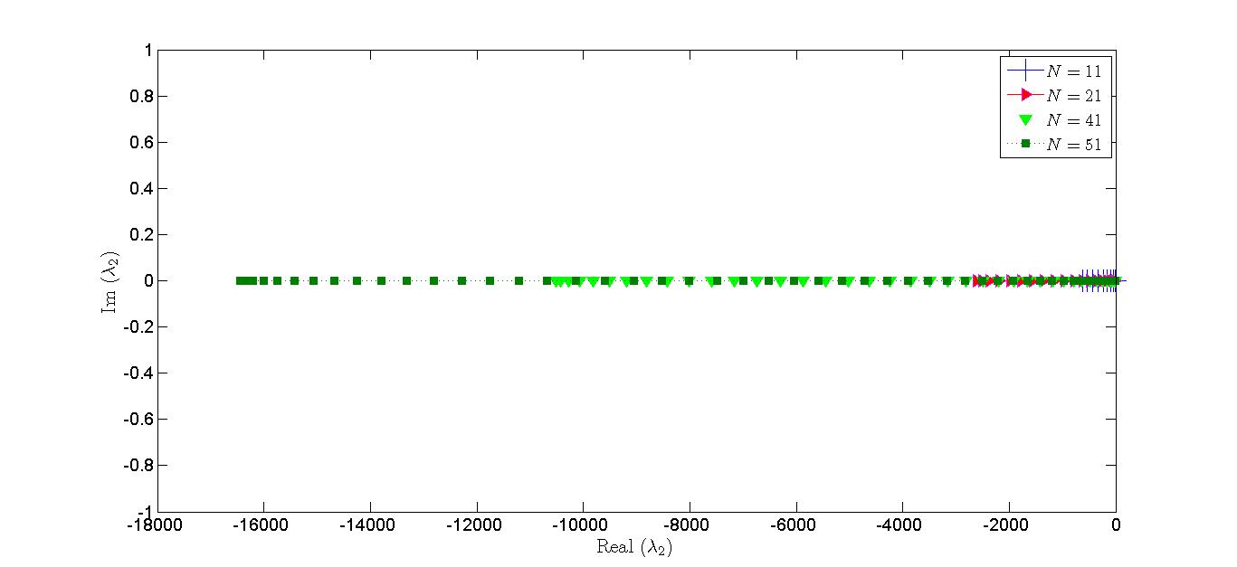
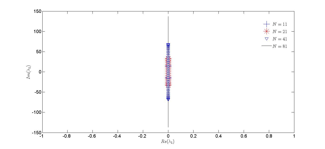
It is seen that the eigenvalues of the matrices Arsubscript𝐴𝑟A_{r} and Brsubscript𝐵𝑟B_{r} (r=1,2)𝑟12(r=1,2) have identical nature. Therefore, it is sufficient to compute the eigenvalues, λ1subscript𝜆1\lambda_{1} and λ2subscript𝜆2\lambda_{2}, of the matrices A1subscript𝐴1A_{1} and A2subscript𝐴2A_{2} for different values of grid sizes (Nx×Ny)subscript𝑁𝑥subscript𝑁𝑦(N_{x}\times N_{y}). The eigenvalues λ1subscript𝜆1\lambda_{1} and λ2subscript𝜆2\lambda_{2} for Nx=Ny=11,21,31,41formulae-sequencesubscript𝑁𝑥subscript𝑁𝑦11213141N_{x}=N_{y}=11,21,31,41 has been depicted in Figure 4. Analogously, one can compute the eigenvalues λ1subscript𝜆1\lambda_{1} and λ2subscript𝜆2\lambda_{2} using mECDQ method [36] or mExp-DQM. It is seen that in either case, λ1subscript𝜆1\lambda_{1} and λ2subscript𝜆2\lambda_{2} have same nature as in Figure 4. Further, we can get from Figure 4 that each eigenvalue λBsubscript𝜆𝐵\lambda_{B} of the matrix B𝐵B as defined in Eq. (69) is real and negative. This confirms that the proposed methods produces stable solutions for two dimensional convection-diffusion equations.

5 Numerical results and discussions

This section deals with the main goal, the numerical study of three test problems of the initial value system of convection-diffusion equations with both kinds of the boundary conditions has been done by adopting the methods MTB-DQM, mExp-DQM and mECDQ method along with the integration SSP-RK54 scheme. The accuracy and the efficiency of the methods have been measured in terms of the discrete error norms: namely- average |error|error|\mbox{error}| norm (L2superscript𝐿2L^{2}-error norm) and the maximum error (Lsubscript𝐿L_{\infty} error norm).

Problem 1

Consider the initial value system of 222D convection-diffusion equation (1) with u0(x,y)=exp{(xx0)2αx(yy0)2αy}subscript𝑢0𝑥𝑦superscript𝑥subscript𝑥02subscript𝛼𝑥superscript𝑦subscript𝑦02subscript𝛼𝑦u_{0}(x,y)=\exp\left\{-\frac{(x-x_{0})^{2}}{\alpha_{x}}-\frac{(y-y_{0})^{2}}{\alpha_{y}}\right\}, while values of fisubscript𝑓𝑖f_{i} for 1i41𝑖41\leq i\leq 4 can be extracted from the exact solution

u(x,y,t)=11+4texp{(xx0βxt)2αx(1+4t)(yy0βyt)2αy(1+4t)},𝑢𝑥𝑦𝑡114𝑡superscript𝑥subscript𝑥0subscript𝛽𝑥𝑡2subscript𝛼𝑥14𝑡superscript𝑦subscript𝑦0subscript𝛽𝑦𝑡2subscript𝛼𝑦14𝑡u(x,y,t)=\frac{1}{{1+4t}}\exp\left\{-\frac{(x-x_{0}-\beta_{x}t)^{2}}{\alpha_{x}(1+4t)}-\frac{(y-y_{0}-\beta_{y}t)^{2}}{\alpha_{y}(1+4t)}\right\},

where initial condition is a Gaussian pulse with unit hight centered at (x0,y0)=(0.5,0.5)subscript𝑥0subscript𝑦00.50.5(x_{0},y_{0})=(0.5,0.5).

We have computed the numerical solution of Problem 1 for βx=βy=0.8subscript𝛽𝑥subscript𝛽𝑦0.8\beta_{x}=\beta_{y}=0.8 and different values of αx,αysubscript𝛼𝑥subscript𝛼𝑦\alpha_{x},\alpha_{y}.

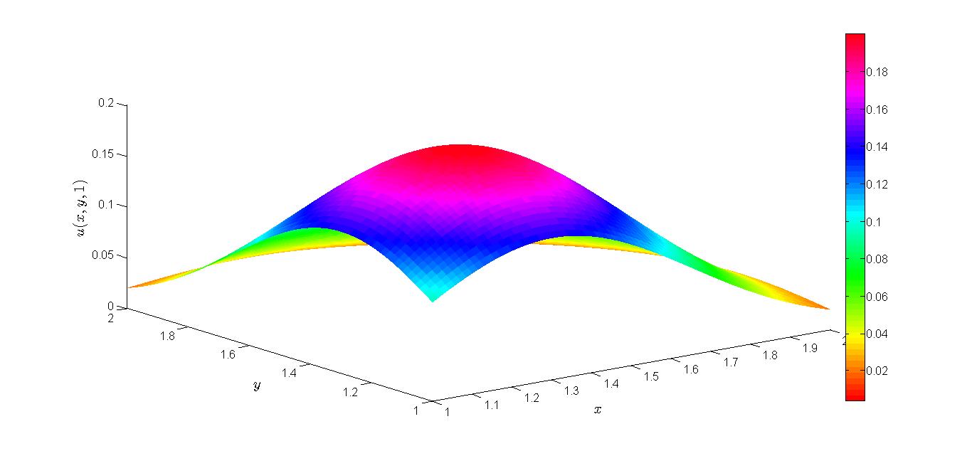
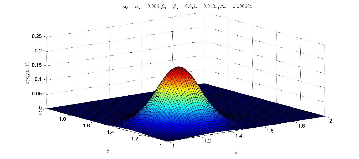
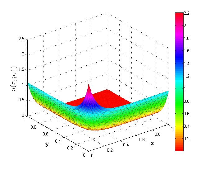
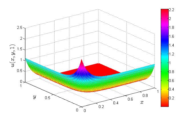
For Ω=[1,2]2Ωsuperscript122\Omega=[1,2]^{2}: Lsubscript𝐿L_{\infty} errors and the rate of convergence (ROC) [36] at t=1𝑡1t=1 for different values of h2=tsuperscript2𝑡h^{2}=\triangle t (hx=hy=hsubscript𝑥subscript𝑦h_{x}=h_{y}=h) has been reported in Table 1 for αx=αy=0.05,0.005formulae-sequencesubscript𝛼𝑥subscript𝛼𝑦0.050.005\alpha_{x}=\alpha_{y}=0.05,0.005. Table 1 confirms that the proposed solutions obtained by these methods are more accurate, and approaching towards exact solutions. The behavior of the approximate solution at time t=1𝑡1t=1 taking h=0.0125,t=0.000625formulae-sequence0.0125𝑡0.000625h=0.0125,\triangle t=0.000625 is depicted in Figure 4 for αx=αy=0.05subscript𝛼𝑥subscript𝛼𝑦0.05\alpha_{x}=\alpha_{y}=0.05 and in Figure 4 for αx=αy=0.005subscript𝛼𝑥subscript𝛼𝑦0.005\alpha_{x}=\alpha_{y}=0.005.

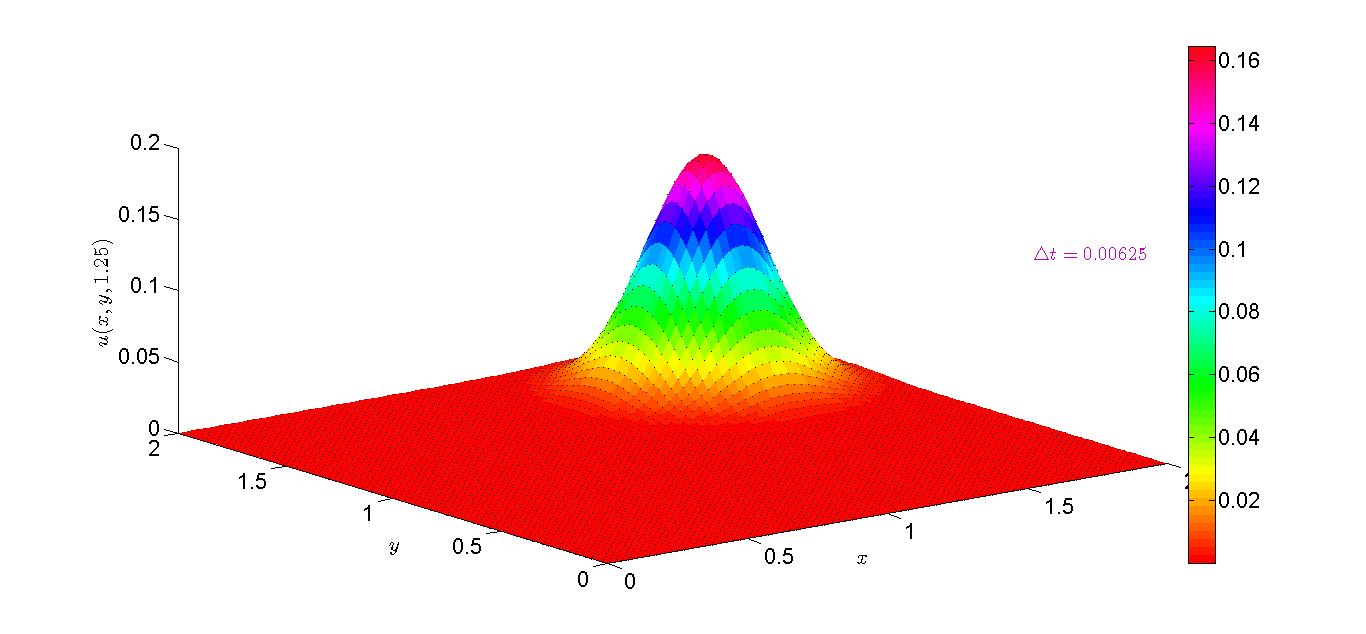
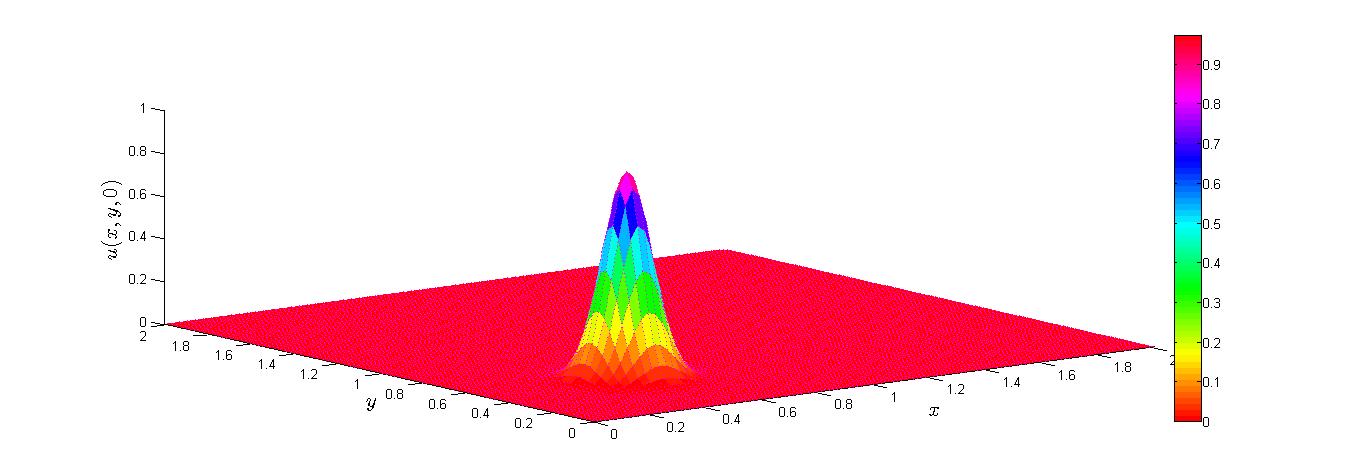
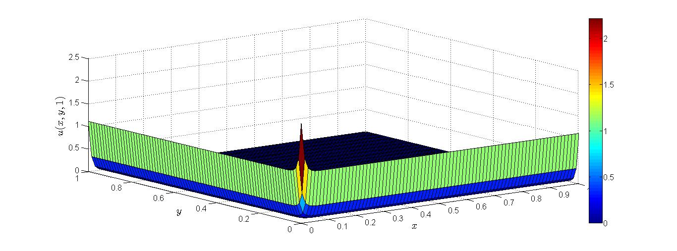
For Ω=[0,2]2Ωsuperscript022\Omega=[0,2]^{2}, time t=1.25𝑡1.25t=1.25, and grid space step size h=0.0250.025h=0.025: the L2superscript𝐿2L^{2} and Lsubscript𝐿L_{\infty} error norms in the proposed solutions have been compared with the errors in the solutions by various schemes in [31, 22, 17, 18, 31, 12] in Table 2 for t=0.00625𝑡0.00625\triangle t=0.00625 and in Table 3 for t=0.0125𝑡0.0125\triangle t=0.0125. The initial solution and MTB-DQM solutions in [0,2]2superscript022[0,2]^{2} with the parameter values αx=αy=0.01,t=1.25formulae-sequencesubscript𝛼𝑥subscript𝛼𝑦0.01𝑡1.25\alpha_{x}=\alpha_{y}=0.01,t=1.25 have been depicted in Figure 4, and similar behavior is seen from the other two methods. It is evident from the above reports that the proposed results are more accurate as compared to [31, 22, 17, 18, 31, 12] and approaching towards the exact solutions.

Table 1: Rate of convergence of Lsubscript𝐿L_{\infty} error norms in Problem 1 in [1,2]2superscript122[1,2]^{2} with αx=αy=0.05,0.005,βx=βy=0.8formulae-sequencesubscript𝛼𝑥subscript𝛼𝑦0.050.005subscript𝛽𝑥subscript𝛽𝑦0.8\alpha_{x}=\alpha_{y}=0.05,0.005,\beta_{x}=\beta_{y}=0.8 taking t=h2𝑡superscript2\triangle t=h^{2} and various grid sizes Nx×Nysubscript𝑁𝑥subscript𝑁𝑦N_{x}\times N_{y} with Nx=Nysubscript𝑁𝑥subscript𝑁𝑦N_{x}=N_{y}
αx=αy=0.005subscript𝛼𝑥subscript𝛼𝑦0.005\alpha_{x}=\alpha_{y}=0.005
Nxsubscript𝑁𝑥N_{x} MTB-DQM mExp-DQM (p=0.001) mECDQ (λ=0.30)𝜆0.30(\lambda=-0.30)
Lsubscript𝐿L_{\infty} ROC Lsubscript𝐿L_{\infty} ROC Lsubscript𝐿L_{\infty} ROC
5 2.91E-03 2.91E-03 1.94E-03
10 6.41E-04 2.18 6.42E-04 2.181 4.93E-04 1.98
20 6.50E-05 3.30 6.51E-05 3.303 6.05E-05 3.03
40 7.19E-06 3.18 7.18E-06 3.180 6.91E-06 3.13
80 7.22E-07 3.31 7.00E-07 3.358 6.99E-07 3.31
αx=αy=0.05subscript𝛼𝑥subscript𝛼𝑦0.05\alpha_{x}=\alpha_{y}=0.05
5 4.93E-04 4.97E-04 3.20E-04
10 4.86E-05 3.34 4.87E-05 3.35 4.39E-05 2.87
20 4.70E-06 3.37 4.70E-06 3.37 4.35E-06 3.34
40 4.51E-07 3.38 4.46E-07 3.40 4.50E-07 3.27
80 4.58E-08 3.30 3.49E-08 3.67 4.37E-08 3.36
Table 2: Comparison L2superscript𝐿2L^{2} and Lsubscript𝐿L_{\infty} error norms for Problem 1 with αx=αy=0.01;βx=βy=0.8formulae-sequencesubscript𝛼𝑥subscript𝛼𝑦0.01subscript𝛽𝑥subscript𝛽𝑦0.8\alpha_{x}=\alpha_{y}=0.01;\beta_{x}=\beta_{y}=0.8 for hx=hy=0.025,t=0.00625formulae-sequencesubscript𝑥subscript𝑦0.025𝑡0.00625h_{x}=h_{y}=0.025,\triangle t=0.00625
Schemes L2superscript𝐿2L^{2} Lsubscript𝐿L_{\infty}
P-R-ADI [31] 3.109E-04              7.778E-03
Noye &\& Tang [22] 1.971E-05 6.509E-04
Kalila et al. [17] 1.597E-05 4.447E-04
Kara &\& Zhang ADI [18] 9.218E-06 2.500E-04
Tang &\& Ge ADI[31] 9.663E-06 2.664E-04
Dehghan &\& Mohebbi [12]             9.431E-06 2.477E-04
MTB-DQM 8.026E-12 4.327E-08
mExp-DQM(p=0.0001) 7.030E-12 4.154E-08
mECDQ (λ=0.004𝜆0.004\lambda=-0.004) 4.504E-12 3.343E-08
MCB-DQM (λ=0𝜆0\lambda=0) 8.269E-12 4.388E-08
Table 3: Comparison L2superscript𝐿2L^{2} and Lsubscript𝐿L_{\infty} error norms for Problem 1 with αx=αy=0.01;βx=βy=0.8formulae-sequencesubscript𝛼𝑥subscript𝛼𝑦0.01subscript𝛽𝑥subscript𝛽𝑦0.8\alpha_{x}=\alpha_{y}=0.01;\beta_{x}=\beta_{y}=0.8 for hx=hy=0.025,t=0.0125formulae-sequencesubscript𝑥subscript𝑦0.025𝑡0.0125h_{x}=h_{y}=0.025,\triangle t=0.0125
Schemes L2superscript𝐿2L^{2} Lsubscript𝐿L_{\infty}
Noye &\& Tang [22] 1.430E-05 4.840E-04
Kalila et al.[17] 1.590E-05 4.480E-04
Dehghan &\& Mohebbi [12]              9.480E-06                           2.469E-04
MTB-DQM 8.900E-12 4.501E-08
mExp-DQM(p=0.0001) 9.147E-12 4.315E-08
mECDQ (λ=0.005𝜆0.005\lambda=-0.005) 4.646E-12 3.852E-08
MCB-DQM (λ=0𝜆0\lambda=0) 9.147E-12 4.561E-08
Problem 2

Consider the initial value system (1) of 222D convection-diffusion equation with Ω=[0,1]2Ωsuperscript012\Omega=[0,1]^{2} with u0(x,y)=a(exp(cxx)+exp(cyy))subscript𝑢0𝑥𝑦𝑎subscript𝑐𝑥𝑥subscript𝑐𝑦𝑦u_{0}(x,y)=a\left(\exp(-c_{x}x)+\exp(-c_{y}y)\right), where

cx=βx±βx2+4bαx2αx>0, and cy=βy±βy2+4bαy2αy>0,formulae-sequencesubscript𝑐𝑥plus-or-minussubscript𝛽𝑥superscriptsubscript𝛽𝑥24𝑏subscript𝛼𝑥2subscript𝛼𝑥0 and subscript𝑐𝑦plus-or-minussubscript𝛽𝑦superscriptsubscript𝛽𝑦24𝑏subscript𝛼𝑦2subscript𝛼𝑦0c_{x}=\frac{-\beta_{x}\pm\sqrt{\beta_{x}^{2}+4b\alpha_{x}}}{2\alpha_{x}}>0,\mbox{ and }c_{y}=\frac{-\beta_{y}\pm\sqrt{\beta_{y}^{2}+4b\alpha_{y}}}{2\alpha_{y}}>0,

and the Neumann boundary condition

{ux|x=0,y=acxexp(bt),ux|x=2,y=acxexp(btcx),uy|x,y=0=acyexp(bt),uy|x,y=2=acyexp(btcy),(x,y,t)Ω×(0,T],\left\{\begin{split}&\left.\frac{\partial u}{\partial x}\right|_{x=0,y}=-ac_{x}\exp(bt),\quad\left.\frac{\partial u}{\partial x}\right|_{x=2,y}=-ac_{x}\exp(bt-c_{x}),\\ &\left.\frac{\partial u}{\partial y}\right|_{x,y=0}=-ac_{y}\exp(bt),\quad\left.\frac{\partial u}{\partial y}\right|_{x,y=2}=-ac_{y}\exp(bt-c_{y}),\end{split}\right.\qquad\quad(x,y,t)\in\partial\Omega\times(0,T],

or the Dirichlet’s conditions can be extracted from the exact solution [8]:

u(x,y,t)=aexp(bt)(exp(cxx)+exp(cyy)).𝑢𝑥𝑦𝑡𝑎𝑏𝑡subscript𝑐𝑥𝑥subscript𝑐𝑦𝑦u(x,y,t)=a\exp(bt)\left(\exp(-c_{x}x)+\exp(-c_{y}y)\right).

The computation by the proposed methods has been done for different values of αx=αysubscript𝛼𝑥subscript𝛼𝑦\alpha_{x}=\alpha_{y} and βx=βysubscript𝛽𝑥subscript𝛽𝑦\beta_{x}=\beta_{y}.

For βx=βy=1subscript𝛽𝑥subscript𝛽𝑦1\beta_{x}=\beta_{y}=1, we take t=0.001𝑡0.001\triangle t=0.001 for the solutions at t=1𝑡1t=1. The rate of convergence and L2superscript𝐿2L^{2} error norms in the proposed solutions has been compared with that of due to fourth-order compact finite difference scheme [12] for αx=αy=0.1,0.01formulae-sequencesubscript𝛼𝑥subscript𝛼𝑦0.10.01\alpha_{x}=\alpha_{y}=0.1,0.01, in Table 4. It is found that the proposed solutions from either method are more accurate in comparison to [12], and are in good agreement with the exact solutions.

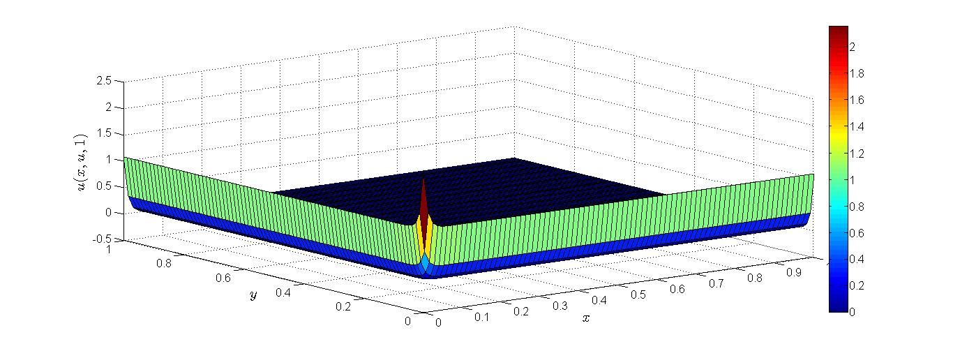
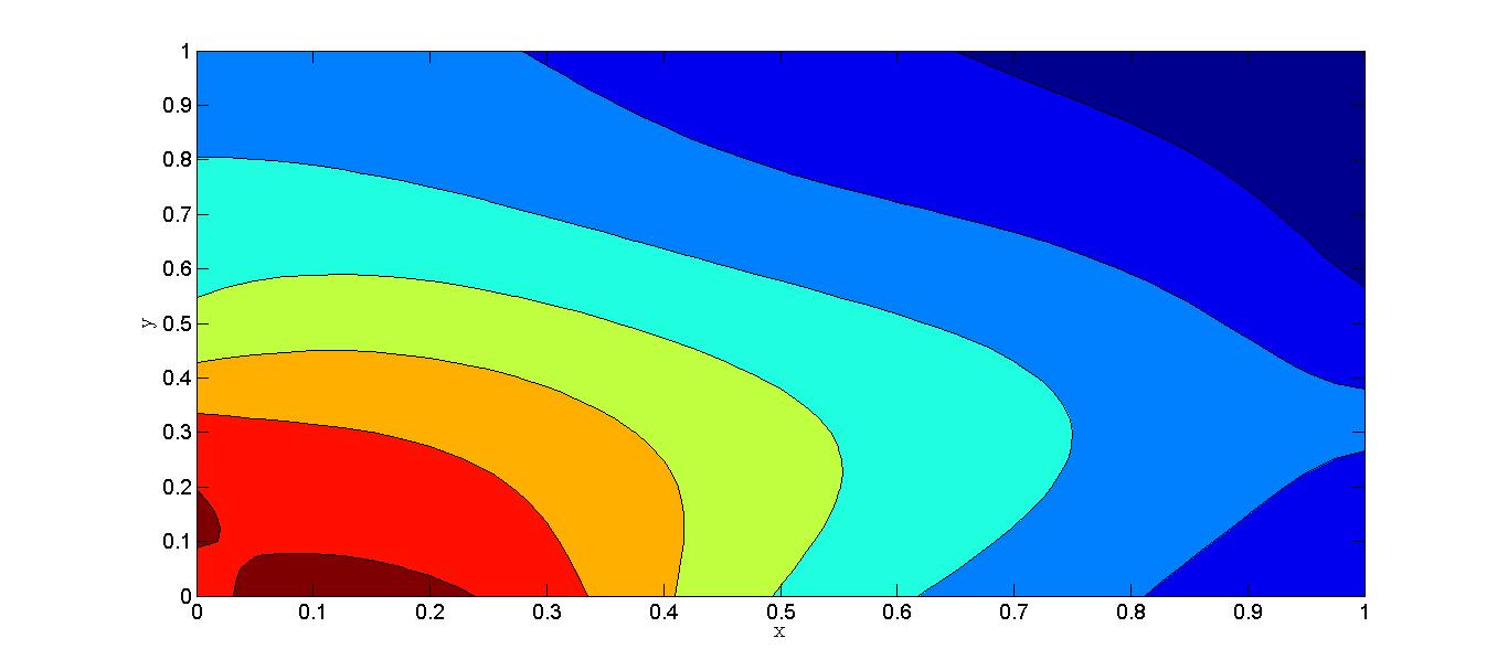
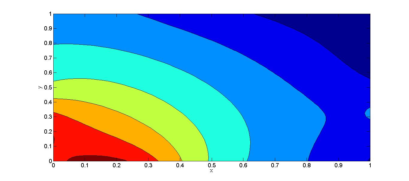
For βx=βy=1subscript𝛽𝑥subscript𝛽𝑦1\beta_{x}=\beta_{y}=-1, we take t=0.0005𝑡0.0005\triangle t=0.0005 for the solution at t=1𝑡1t=1. In Table 5, the L2superscript𝐿2L^{2} and Lsubscript𝐿L_{\infty} error norms are compared with that obtained by fourth-order compact finite difference scheme [12] for βx=βy=1subscript𝛽𝑥subscript𝛽𝑦1\beta_{x}=\beta_{y}=-1, and αx=αy=0.01subscript𝛼𝑥subscript𝛼𝑦0.01\alpha_{x}=\alpha_{y}=0.01. Rate of convergence have been reported in Table 6. From Tables 5 and 6, we found that the proposed solutions are more accurate as compared to the results in [12], while the rate of convergence is linear. The behavior of solutions is depicted in Figure 7 and 7 with h=0.0250.025h=0.025 for αx=αy=0.1subscript𝛼𝑥subscript𝛼𝑦0.1\alpha_{x}=\alpha_{y}=0.1 and αx=αy=0.01subscript𝛼𝑥subscript𝛼𝑦0.01\alpha_{x}=\alpha_{y}=0.01, respectively.

For the same parameter, mentioned above, the numerical solution is obtained by using Neumann conditions and reported in Table 7. The obtained results are in good agreement with the exact solutions, the rate of convergence for L𝐿L\infty is quadratic for each method.

Table 4: L2superscript𝐿2L^{2}-error norms and ROC for Problem 2 with βx=βy=1subscript𝛽𝑥subscript𝛽𝑦1\beta_{x}=\beta_{y}=1 and αx=αy=0.10,0.01formulae-sequencesubscript𝛼𝑥subscript𝛼𝑦0.100.01\alpha_{x}=\alpha_{y}=0.10,0.01 at t=1𝑡1t=1
αx=αy=0.10subscript𝛼𝑥subscript𝛼𝑦0.10\alpha_{x}=\alpha_{y}=0.10 and t=0.0005𝑡0.0005\triangle t=0.0005
MTB-DQM mExp-DQM (p=1)𝑝1(p=1) mECDQ (λ=0.0001)𝜆0.0001(\lambda=-0.0001) CFDS4[12]
hh L𝐿L\infty ROC L2superscript𝐿2L^{2} ROC L𝐿L\infty ROC L2superscript𝐿2L^{2} ROC L𝐿L\infty ROC L2superscript𝐿2L^{2} ROC L2superscript𝐿2L^{2} ROC
0.2 4.231E-06 4.969E-10 1.714E-05 3.584E-09 4.231E-06 4.999E-10
0.1 5.155E-07 3.0 2.472E-11 4.3 5.168E-07 5.1 2.473E-11 7.2 5.153E-07 3.0 2.478E-11 4.3 2.289E-10
0.05 5.108E-08 3.3 9.041E-13 4.8 5.105E-08 3.3 9.044E-13 4.8 5.107E-08 3.3 9.049E-13 4.8 1.621E-11 3.82
0.025 1.147E-08 2.2 1.922E-14 5.6 1.147E-08 2.2 1.922E-14 5.6 1.147E–08 2.4 1.923E-14 5.6 8.652E-13 4.23
αx=αy=0.01,t=0.001formulae-sequencesubscript𝛼𝑥subscript𝛼𝑦0.01𝑡0.001\alpha_{x}=\alpha_{y}=0.01,\triangle t=0.001
0.2 7.4031E-06 1.4907E-09 3.5634E-05 1.5314E-08 2.0585E-06 6.7290E-11
0.1 1.1460E-06 2.7 1.3103E-10 3.5 1.1421E-06 5.0 1.3148E-10 6.9 1.5919E-07 3.7 1.1624E-12 5.9 2.749E-09
0.05 1.4578E-07 3.0 7.5377E-12 4.1 1.4582E-07 3.0 7.5396E-12 4.1 1.9012E-08 3.1 5.4939E-14 4.4 2.394E-10 3.52
0.025 1.3902E-08 3.4 2.7129E-13 4.8 1.3904E-08 3.4 2.7132E-13 4.8 6.2220E-09 1.6 9.0456E-15 2.6 1.658E-11 3.85
Table 5: Comparison of the error norms in Problem 2 with βx=βy=1subscript𝛽𝑥subscript𝛽𝑦1\beta_{x}=\beta_{y}=-1, αx=αy=0.01subscript𝛼𝑥subscript𝛼𝑦0.01\alpha_{x}=\alpha_{y}=0.01 taking t=0.0005𝑡0.0005\triangle t=0.0005 with CFDS4[12]
MTB-DQM mExp-DQM,p=0.0001𝑝0.0001p=0.0001 mECDQ,λ=1.75𝜆1.75\lambda=-1.75 CFDS4 [12]
hh Lsubscript𝐿L_{\infty} L2superscript𝐿2L^{2} Lsubscript𝐿L_{\infty} L2superscript𝐿2L^{2} Lsubscript𝐿L_{\infty} L2superscript𝐿2L^{2} Lsubscript𝐿L_{\infty} L2superscript𝐿2L^{2}
0.04 4.1718E-03 1.7833E-03 1.7475E-03 7.9168E-04 1.2939E-03 3.6957E-04 1.1826E-01 4.9331E-03
0.02 5.2095E-04 6.8410E-05 5.2097E-04 6.8445E-05 6.3735E-04 6.8622E-05 1.5310E-02 4.1351E-04
0.01 3.2496E-04 2.1508E-05 3.2484E-04 2.1493E-05 2.5394E-04 1.8260E-05 9.4696E-04 2.8405E-05
Table 6: L2superscript𝐿2L^{2} and L𝐿L\infty error norms in Problem 2 with βx=βy=1subscript𝛽𝑥subscript𝛽𝑦1\beta_{x}=\beta_{y}=-1 and different values of αx=αysubscript𝛼𝑥subscript𝛼𝑦\alpha_{x}=\alpha_{y}
αx=αy=0.01,t=0.0005formulae-sequencesubscript𝛼𝑥subscript𝛼𝑦0.01𝑡0.0005\alpha_{x}=\alpha_{y}=0.01,\triangle t=0.0005
MTB-DQM mExp-DQM,p=0.0001𝑝0.0001p=0.0001 mECDQ, λ=0.9𝜆0.9\lambda=-0.9
hh L𝐿L\infty ROC L2superscript𝐿2L^{2} ROC L𝐿L\infty ROC L2superscript𝐿2L^{2} ROC L𝐿L\infty ROC L2superscript𝐿2L^{2} ROC
0.1 2.6263E-02 3.6277E-02 2.6280E-02 3.6670E-02 2.4464E-02 4.0175E-02
0.05 6.8144E-03 1.9 4.1447E-03 3.1 6.8144E-03 1.9 4.1339E-03 3.1 3.3580E-03 2.9 1.6264E-03 4.6
0.025 1.1634E-03 2.6 2.7780E-04 3.9 1.0719E-03 2.7 1.9697E-04 4.4 8.1776E-04 2.0 1.0090E-04 4.0
αx=αy=0.1,t=0.0005formulae-sequencesubscript𝛼𝑥subscript𝛼𝑦0.1𝑡0.0005\alpha_{x}=\alpha_{y}=0.1,\triangle t=0.0005
p=0.0001𝑝0.0001p=0.0001 λ=0.3𝜆0.3\lambda=0.3
0.01 5.0998E-04 3.5191E-03 5.0738E-04 1.0116E-05 7.4180E-04 2.5558E-05
0.05 1.8776E-04 1.4 1.8193E-03 1.0 1.8776E-04 1.4 2.9979E-06 1.8 2.0972E-04 1.8 5.1381E-06 2.3
0.025 9.9342E-05 0.9 9.1372E-04 1.0 9.9342E-05 0.9 7.9462E-07 1.9 9.5677E-05 1.1 8.1188E-07 2.7
Table 7: The L2superscript𝐿2L^{2}-error norm in Problem 2 with Neumann boundary conditions for the different values of αx,αysubscript𝛼𝑥subscript𝛼𝑦\alpha_{x},\alpha_{y} and βx,βysubscript𝛽𝑥subscript𝛽𝑦\beta_{x},\beta_{y} with t=0.0005𝑡0.0005\triangle t=0.0005
αx=αy=0.1subscript𝛼𝑥subscript𝛼𝑦0.1\alpha_{x}=\alpha_{y}=0.1and βx=βy=1subscript𝛽𝑥subscript𝛽𝑦1\beta_{x}=\beta_{y}=-1
MTB-DQM mExp-DQM,p=0.001𝑝0.001p=0.001 mECDQ, λ=0.9𝜆0.9\lambda=-0.9
hh L𝐿L\infty ROC L2superscript𝐿2L^{2} ROC L𝐿L\infty ROC L2superscript𝐿2L^{2} ROC L𝐿L\infty ROC L2superscript𝐿2L^{2} ROC
0.05 1.0176E-02 6.7504E-03 1.0177E-02 6.7513E-03 9.1549E-03 5.7412E-03
0.025 2.2164E-03 2.2 1.0428E-03 2.7 2.2165E-03 2.2 1.0429E-03 2.7 1.9834E-03 2.2 8.7214E-04 2.7
0.0125 2.9460E-04 2.9 7.2888E-05 3.8 2.9460E-04 2.9 7.2889E-05 3.8 2.5565E-04 3.0 5.6518E-05 3.9
αx=αy=0.01subscript𝛼𝑥subscript𝛼𝑦0.01\alpha_{x}=\alpha_{y}=0.01 and βx=βy=1subscript𝛽𝑥subscript𝛽𝑦1\beta_{x}=\beta_{y}=-1
p=0.001𝑝0.001p=0.001 λ=0.9𝜆0.9\lambda=-0.9
0.05 1.2070E-01 6.3285E-01 1.2070E-01 6.3293E-01 1.0921E-01 6.0454E-01
0.025 2.7808E-02 2.1 6.2302E-02 3.3 2.7809E-02 2.1 6.2304E-02 3.3 2.6004E-02 2.1 5.5004E-02 3.5
0.0125 6.0348E-03 2.2 6.4433E-03 3.3 6.0348E-03 2.2 6.4433E-03 3.3 5.4733E-03 2.2 5.5668E-03 3.3
αx=αy=0.1subscript𝛼𝑥subscript𝛼𝑦0.1\alpha_{x}=\alpha_{y}=0.1 and βx=βy=1subscript𝛽𝑥subscript𝛽𝑦1\beta_{x}=\beta_{y}=1
p=0.01 λ=0.9𝜆0.9\lambda=-0.9
0.05 1.4931E-05 5.8044E-08 1.4932E-05 5.8056E-08 1.3598E-05 4.8332E-08
0.025 3.3009E-06 2.2 1.0664E-08 2.4 3.3009E-06 2.2 1.0665E-08 2.4 2.9824E-06 2.2 8.7286E-09 2.5
0.0125 4.5947E-07 2.8 8.0780E-10 3.7 4.5947E-07 2.8 8.0780E-10 3.7 3.9840E-07 2.9 6.0761E-10 3.8
αx=αy=0.01subscript𝛼𝑥subscript𝛼𝑦0.01\alpha_{x}=\alpha_{y}=0.01 and βx=βy=1subscript𝛽𝑥subscript𝛽𝑦1\beta_{x}=\beta_{y}=1
p=0.01 λ=0.9𝜆0.9\lambda=-0.9
0.05 1.7132E-05 6.9905E-08 1.7132E-05 6.9910E-08 1.6511E-05 6.5219E-08
0.025 3.9931E-06 2.1 1.4135E-08 2.3 3.9932E-06 2.1 1.4136E-08 2.3 3.7892E-06 2.1 1.2756E-08 2.4
0.0125 8.8931E-07 2.2 2.7052E-09 2.4 8.8931E-07 2.2 2.7052E-09 2.4 8.2511E-07 2.2 2.3316E-09 2.5
Problem 3

The initial value system of 222D convection-diffusion equation (1) with Ω=[0,1]2Ωsuperscript012\Omega=[0,1]^{2} and u0(x,y)=h(x,y)subscript𝑢0𝑥𝑦𝑥𝑦u_{0}(x,y)=h(x,y), and

f1=h(0,y)c¯t;f1=h(1,y)c¯t;f3==h(x,0)c¯t;f4=h(x,1)c¯t,\begin{split}&f_{1}=h(0,y)-\overline{c}t;\quad f_{1}=h(1,y)-\overline{c}t;\quad f_{3}==h(x,0)-\overline{c}t;\quad f_{4}=h(x,1)-\overline{c}t,\end{split}

where

h(x,y)=5exp{(9x2)24(9y2)24}+7exp{(9x+1)250(9y+1)10}+4exp{(9x7)24(9y3)24}2exp{(9x4)2(9y7)2}𝑥𝑦5superscript9𝑥224superscript9𝑦2247superscript9𝑥12509𝑦1104superscript9𝑥724superscript9𝑦3242superscript9𝑥42superscript9𝑦72\begin{split}h(x,y)&=5\exp\left\{-\frac{(9x-2)^{2}}{4}-\frac{(9y-2)^{2}}{4}\right\}+7\exp\left\{-\frac{(9x+1)^{2}}{50}-\frac{(9y+1)}{10}\right\}\\ &\qquad+4\exp\left\{-\frac{(9x-7)^{2}}{4}-\frac{(9y-3)^{2}}{4}\right\}-2\exp\left\{-(9x-4)^{2}-(9y-7)^{2}\right\}\end{split}

The distribution of the initial solution is depicted in Figure LABEL:ex3-fig3.1. The solutions behavior is obtained for the parameter values: αx=0.2,αy=0.3,βx=0.1,βy=0.2formulae-sequencesubscript𝛼𝑥0.2formulae-sequencesubscript𝛼𝑦0.3formulae-sequencesubscript𝛽𝑥0.1subscript𝛽𝑦0.2\alpha_{x}=0.2,\alpha_{y}=0.3,\beta_{x}=-0.1,\beta_{y}=0.2 and t=0.0005,hx=hy=0.025formulae-sequence𝑡0.0005subscript𝑥subscript𝑦0.025\triangle t=0.0005,h_{x}=h_{y}=0.025, and is depicted in Figure 7 due to MTB-DQM, also we noticed the similar characteristics obtained using mExp-DQM and mECDQ method. The obtained characteristics agreed well as obtained in [12, 34].

6 Conclusions

In this paper, the numerical computations of initial value system of two dimensional convection-diffusion equations with both kinds of boundary conditions has been done by adopting three methods: modified exponential cubic B-splines DQM, modified trigonometric cubic B-splines DQM, and mECDQ method [36], which transforms the convection-diffusion equation into a system of first order ordinary differential equations (ODEs), in time, which is solved by using SSP-RK54 scheme.

The methods are found stable for two space convection-diffusion equation by employing matrix stability analysis method. Section 5 shows that the proposed solutions are more accurate in comparison to the solutions by various existing schemes, and are in good agreement with the exact solutions.

The order of accuracy of the proposed methods for the convection-diffusion problem with Dirichlet’s boundary conditions is cubic whenever βx,βy>0subscript𝛽𝑥subscript𝛽𝑦0\beta_{x},\beta_{y}>0 and otherwise it is super linear, in space. On the other hand, the order of accuracy of the proposed methods for the convection-diffusion problem with Neumann boundary condition is quadratic with respect to L2subscript𝐿2L_{2} error norms, see Table 7.

References

  • [1] G. Arora and B. K. Singh, Numerical solution of Burgers’ equation with modified cubic B-spline differential quadrature method. Applied Math Comput 224 (2013) 166-177.
  • [2] B. K. Singh and G. Arora, A numerical scheme to solve Fisher-type reaction-diffusion equations, Nonlinear Studies/MESA- MATHEMATICS IN ENGINEERING, SCIENCE AND AEROSPACE 5(2) (2014) 153–164.
  • [3] B. K. Singh, G. Arora, M. K. Singh, A numerical scheme for the generalized Burgers-Huxley equation, Journal of the Egyptian Mathematical Society (2016) http://dx.doi.org/10.1016/j.joems.2015.11.003.
  • [4] B. K. Singh and Carlo Bianca, A new numerical approach for the solutions of partial differential equations in three-dimensional space, Appl. Math. Inf. Sci. 10, No. 5, 1-10 (2016).
  • [5] R. Bellman, B.G. Kashef and J. Casti, Differential quadrature: a technique for the rapid solution of nonlinear differential equations. J Comput Phy 10 (1972) 40-52.
  • [6] Huai-Huo Cao, Li-Bin Liu, Yong Zhang and Sheng-mao Fu, A fourth-order method of the convection-diffusion equations with Neumann boundary conditions, Applied Mathematics and Computation 217 (2011) 9133-9141.
  • [7] M.M. Cecchi and M.A. Pirozzi, High order finite difference numerical methods for time-dependent convecion-dominated problems, Appl. Numer. Math. 55 (2005) 334-356.
  • [8] P.P. Chinchapatnam, K. Djidjeli and P.B. Nair, Unsymmetric and symmetric meshless schemes for the unsteady convection-diffusion equation, Comput. Methods Appl. Mech. Eng. 195 (2006) 2432-2453.
  • [9] S. P. Dawson, S. Chen and G. D. Doolen, Lattice Boltzmann computations for reaction-diffusion equations, J. Chem. Phys. 98 (2) (1993) 1514-1523.
  • [10] M. Dehghan, Weighted finite difference techniques for the one-dimensional advection-diffusion equation, Appl. Math. Comput. 147 (2004) 307-319.
  • [11] M. Dehghan, Numerical solution of the three-dimensional advection-diffusion equation, Appl. Math. Comput. 150 (2004) 5-19.
  • [12] M. Dehghan and A. Mohebbi, High-order compact boundary value method for the solution of unsteady convection-diffusion problems, Math. Comput. Simulat. 79 (2008) 683-699.
  • [13] S. Dhawan, S. Kapoor and S. Kumar, Numerical method for advection diffusion equation using FEM and B-splines, Journal of Computational Science 3 (2012) 429-437.
  • [14] Hengfei Ding and Yuxin Zhang, A new difference scheme with high accuracy and absolute stability for solving convection-diffusion equations, Journal of Computational and Applied Mathematics 230 (2009) 600-606.
  • [15] M.M. Gupta, R.P. Manohar and J.W. Stephenson, A single cell high-order scheme for the convection-diffusion equation with variable coefficients, Int. J. Numer. Methods Fluids 4 (1984) 641-651.
  • [16] M.K. Jain, Numerical Solution of Differential Equations, 2nd Ed., Wiley, New York, NY, 1983.
  • [17] J.C. Kalita, D.C. Dalal and A.K. Dass, A class of higher order compact schemes for the unsteady two-dimensional convection-diffusion equation with variable convection coefficients, Int. J. Numer. Methods Fluids 38 (2002) 1111-1131.
  • [18] S. Karaa and J.Zhang, High order ADI method for solving unsteady convection-diffusion problems, J. Comput. Phys. 198 (2004)1-9.
  • [19] Korkmaz A. Shock wave simulations using sinc differential quadrature method. Int J Comput Aided Engg Software 28(6) (2011) 654-674.
  • [20] A. Mohebbi and M. Dehghan, High-order compact solution of the one-dimensional heat and advection-diffusion equations, Applied Mathematical Modelling 34 (2010) 3071-3084
  • [21] B.J. Noye, A compact unconditionally stable finite-difference method for transient one-dimensional advection-diffusion, Commun. Appl. Numer. Methods 7 (1991) 501-512.
  • [22] B.J. Noye and H.H. Tan, Finite difference methods for solving the two-dimensional advection-diffusion equation, Int. J. Numer. Methods Fluids,26 (1988) 1615-1629.
  • [23] W.F. Spotz, High-order Compact Finite Difference Schemes for Computational Mechanics, PhD Thesis, University of Texas at Austin, Austin, TX, 1995.
  • [24] J.R. Quan and C.T. Chang, New insights in solving distributed system equations by the quadrature methods-I. Comput Chem Eng 13(1989) 779-788.
  • [25] J.R. Quan and C.T. Chang, New insights in solving distributed system equations by the quadrature methods-II. Comput Chem Eng 13 (1989) 1017-1024.
  • [26] P. J. Roach, Computational Fluid Dynamics, Hermosa Press, Albuquerque, NM, 1976.
  • [27] C. Shu and B. E. Richards, Application of generalized differential quadrature to solve two dimensional incompressible Navier-Stokes equations. Int J Numer Meth Fluids 15 (1992) 791-8.
  • [28] C. Shu, Differential Quadrature and its Application in Engineering. Athenaeum Press Ltd., Great Britain, 2000.
  • [29] W.F. Spotz and G.F. Carey, Extension of high-order compact schemes to time-dependent problems, Numer. Methods Partial Diff. Eq. 17 (2001) 657-672.
  • [30] Zhen F. Tian, A rational high-order compact ADI method for unsteady convection-diffusion equations, Computer Physics Communications 182 (2011) 649–662.
  • [31] Z.F. Tian and Y.B. Ge, A fourth-order compact ADI method for solving two-dimensional unsteady convection-diffusion problems, J. Comput. Appl. Math. 198 (2007) 268-286.
  • [32] Zhen F. Tian and P. X. Yua, A high-order exponential scheme for solving 1D unsteady convection-diffusion equations, Journal of Computational and Applied Mathematics 235 (2011) 2477-2491.
  • [33] Donghyun You, A high-order Pade’ ADI method for unsteady Convection-diffusion equations, Journal of Computational Physics 214 (2006) 1-11
  • [34] M. Zerroukat, K. Djidjeli and A. Charafi, Explicit and implicite messless method for linear advection-diffusion-type partial differential eqations, International Journal Numerical Method in Engineering 48 (2000) 19-35.
  • [35] G. Arora, V. Joshi, A computational approach for solution of one dimensional parabolic partial differential equation with application in biological processes, Ain Shams Eng J (2016), http://dx.doi.org/10.1016/j.asej.2016.06.013.
  • [36] B.K. Singh, P. Kumar, A novel approach for numerical computation of Burgers’ equation (1+1)11(1+1) and (2+1)21(2+1) dimension, Alexandria Eng. J. (2016), http://dx.doi.org/10.1016/j.aej.2016.08.023.
  • [37] B.K. Singh, P. Kumar, An algorithm based on a new DQM with modified extended cubic B-splines for numerical study of two dimensional hyperbolic telegraph equation, Alexandria Eng. J. (2016), http://dx.doi.org/10.1016/j.aej.2016.11.009.
  • [38] G. Arora, RC Mittal and B. K. Singh, Numerical Solution of BBM-Burger Equation with Quartic B-spline collocation method, Journal of Engineering Science and Technology, Special Issue 1, 12/2014, 104 - 116.
  • [39] V. K. Srivastava and B. K. Singh, A Robust finite difference scheme for the numerical solutions of two dimensional time-dependent coupled nonlinear Burgers’ equations, International Journal of Applied Mathematics and Mechanics 10(7) (2014) 28-39.
  • [40] A. Korkmaz, and H. K. Akmaz, Numerical Simulations for Transport of Conservative Pollutants. Selcuk Journal of Applied Mathematics 16(1) (2015).
  • [41] Ozlem Ersoy and Idris Dag, Numerical solutions of the reaction diffusion system by using exponential cubic B-spline collocation algorithms, Open Phys. 13(2015)414-427.
  • [42] A. Korkmaz and H.K. Akmaz, Extended B-spline Differential Quadrature Method for Nonlinear Viscous Burgers’ Equation, Proceedings of International Conference on Mathematics and Mathematics Education, pp 323-323, Elaziǧ, Turkey 12-14 May, 2016.
  • [43] Muhammad Abbas, Ahmad Abd. Majid, Ahmad Izani Md. Ismail, Abdur Rashid, The application of cubic trigonometric B-spline to the numerical solution of the hyperbolic problems, Applied Mathematics and Computation 239 (2014) 74-88.
  • [44] M.K. Jain, Numerical Solution of Differential Equations, 2nd ed., Wiley, New York, NY, 1983.
  • [45] S. Gottlieb, D. I. Ketcheson, C. W. Shu, High Order Strong Stability Preserving Time Discretizations, J. Sci. Comput. 38 (2009) 251-289.
  • [46] J. R. Spiteri and S. J. Ruuth, A new class of optimal high-order strongstability-preserving time-stepping schemes. SIAM Journal Numer Anal 40(2) (2002) 469-491
Refer to caption
Refer to caption
Figure 1: Eigenvalues λ1subscript𝜆1\lambda_{1} and λ2subscript𝜆2\lambda_{2} for different grid sizes
Refer to caption
Figure 2: Surface plot of distribution of 222D convection-diffusion equation (1) with αx=αy=0.05subscript𝛼𝑥subscript𝛼𝑦0.05\alpha_{x}=\alpha_{y}=0.05, βx=βy=0.8subscript𝛽𝑥subscript𝛽𝑦0.8\beta_{x}=\beta_{y}=0.8 at t=1𝑡1t=1
Refer to caption
Figure 3: Surface plot of distribution of 222D convection-diffusion equation (1) with αx=αy=0.005subscript𝛼𝑥subscript𝛼𝑦0.005\alpha_{x}=\alpha_{y}=0.005, βx=βy=0.8subscript𝛽𝑥subscript𝛽𝑦0.8\beta_{x}=\beta_{y}=0.8 at t=1𝑡1t=1
Refer to caption
Refer to caption
Figure 4: Surface plot of the inititial distribution (right) and the distribution at t=1.25𝑡1.25t=1.25 (left) of 2D convection-diffusion equation (1) with αx=αy=0.01subscript𝛼𝑥subscript𝛼𝑦0.01\alpha_{x}=\alpha_{y}=0.01, βx=βy=0.8subscript𝛽𝑥subscript𝛽𝑦0.8\beta_{x}=\beta_{y}=0.8 for hx=hy=0.025subscript𝑥subscript𝑦0.025h_{x}=h_{y}=0.025
Refer to caption
Refer to caption
Figure 5: The approximate (left) and exact solution behavior (right) of 222D convection-diffusion equation (1) with αx=αy=0.10subscript𝛼𝑥subscript𝛼𝑦0.10\alpha_{x}=\alpha_{y}=0.10, βx=βy=1subscript𝛽𝑥subscript𝛽𝑦1\beta_{x}=\beta_{y}=-1 at t=1𝑡1t=1
Refer to caption
Refer to caption
Figure 6: The approximate solution behavior of 222D convection-diffusion equation (1) with αx=αy=0.01subscript𝛼𝑥subscript𝛼𝑦0.01\alpha_{x}=\alpha_{y}=0.01, βx=βy=1subscript𝛽𝑥subscript𝛽𝑦1\beta_{x}=\beta_{y}=-1 at t=1𝑡1t=1
Refer to caption
Refer to caption
Figure 7: The approximate solution behavior of the distribution of 222D convection-diffusion equation (1) in Example 3 at t=0.1𝑡0.1t=0.1 (left) and t=0.5𝑡0.5t=0.5 (right)