General calculation of the cross section for dark matter annihilations into two photons

Abstract

Assuming that the underlying model satisfies some general requirements such as renormalizability and CP conservation, we calculate the non-relativistic one-loop cross section for any self-conjugate dark matter particle annihilating into two photons. We accomplish this by carefully classifying all possible one-loop diagrams and, from them, reading off the dark matter interactions with the particles running in the loop. Our approach is general and leads to the same results found in the literature for popular dark matter candidates such as the neutralinos of the MSSM, minimal dark matter, inert Higgs and Kaluza-Klein dark matter.

I Introduction

Little is known about the nature of Dark Matter (DM), even though its existence has been firmly established by multiple astrophysical and cosmological observations. We know its abundance ( $\Omega_{\text{DM}}h^{2}=0.1197\pm 0.0022$ Ade et al. (2016)), the fact that interacts very weakly with normal matter and that was cold during the time when the first structures formed in the early universe. These properties naturally arise in scenarios where DM is a Weakly Interacting Massive Particle (WIMP) and make the latter very compelling DM models (For reviews see Refs. Bergström (2000); Bertone et al. (2005)). One of the chief predictions of such models is the possibility that DM can annihilate into SM particles. Among these, gamma rays are particularly important because, in contrast to charged particles, they are not deflected when they propagate through astrophysical environments and thus point towards the region where they were produced.

Even more important are gamma-ray lines: since no astrophysical process is known to produce them, the observation of one of them would strongly suggest the existence of WIMP DM, specially if they come from a region where the concentration of DM is known to be high (For a review, see e.g. Ref Bringmann and Weniger (2012)). In fact, the non-observation of statistically significant gamma-ray lines by Fermi-LAT Ackermann et al. (2013, 2015); Liang et al. (2016a); Anderson et al. (2016); Liang et al. (2016b); Profumo et al. (2016) or H.E.S.S. Abramowski et al. (2013); Abdalla et al. (2016) allows to set stringent limits on the DM annihilation cross section into monochromatic photons. Similar limits have been derived using the CMB anisotropies measured by the Planck satellite Slatyer (2016) (and references therein).

Consequently, in a given DM model, it is very important to calculate the cross sections of processes leading to gamma-ray lines. Nevertheless, in contrast to other annihilation channels, this task is not straightforward. Such processes only arise at one-loop level because, typically, DM does not couple to photons. Moreover, the number of Feynman diagrams increases dramatically with the number of charged particles that couple to DM and run in the loop, which leads to annihilation cross sections that are highly dependent on the DM model.

In view of this situation, most of the studies that calculate the annihilation cross section into gamma-ray lines have been based on specific DM models Jackson et al. (2010); Giacchino et al. (2014); Bergstrom et al. (2005); Ibarra et al. (2014); Bertone et al. (2009); Birkedal et al. (2006); Bertone et al. (2012); Arina et al. (2014); Cerdeno et al. (2016); Weiner and Yavin (2012); Tulin et al. (2013); Choi and Seto (2012); Chalons and Semenov (2011); Chalons et al. (2013); Choi and Seto (2012). Early studies focused on certain supersymmetric DM candidates Bergstrom and Snellman (1988); Rudaz (1989); Giudice and Griest (1989); Bergstrom (1989a, b); Bergstrom and Kaplan (1994); Baek et al. (2014), culminating with the works of Refs. Bergstrom and Ullio (1997); Bern et al. (1997); Ullio and Bergstrom (1998), which reported the full one-loop calculation for any neutralino of the MSSM annihilating into one or two photons. Another common approach to gamma-ray lines is based on effective theories where the annihilation into photons arises from high-dimensional operators in such way that microscopic details of the model are integrated out Goodman et al. (2011); Abazajian et al. (2012); Rajaraman et al. (2012); Dudas et al. (2014); El Aisati et al. (2014); Coogan et al. (2015); Duerr et al. (2016a); Arina et al. (2010); Chu et al. (2012); Wang and Han (2013); Bai and Shelton (2012); Fichet (2016); Rajaraman et al. (2013).

In this article, we show that in spite of the complexity of the problem, the cross section for DM annihilations into two photons can be calculated in a general way for any DM model meeting a basic set of requirements. Similar attempts in this direction were done in Refs. Jackson et al. (2013); Duerr et al. (2015) for DM candidates with s-channel mediators, and more generally in Ref. Asano et al. (2013) by means of the optical theorem when the DM particles are heavier than the particles running in the loop.

This paper is organized as follows. We start Sec. II by listing the properties that we assume for the DM, which allows us to determine the corresponding Feynman diagrams. From them, we read off the interactions between DM and the particles in the loop. In Sec. III, we then calculate the annihilation amplitudes and the corresponding cross sections. In Sec. IV, we summarize our findings and illustrate them with examples from popular DM models. In Sec. V, we present our conclusions. Appendices A discusses the gauge choice of the vector particles in our work. Appendix B gives technical details concerning and the Passarino–Veltman functions for box diagrams in the non-relativistic limit. Finally, in Appendix C, we report some formulas needed to compute annihilation amplitudes.

II General properties of the annihilation process DM DM $\to\gamma\gamma$

II.1 Classification of the diagrams

In order to systematically study DM annihilations into two photons, we will assume that the following conditions are satisfied:

1. DM is its own antiparticle and its stability is guaranteed by a $Z_{2}$ symmetry. This implies that DM is electrically neutral and that it can not emit photons.

2. The underlying DM theory is renormalizable. Consequently, any additional neutral particle, including the DM, do not couple to two photons at tree level.

3. In a cubic vertex, photons couple to particles belonging to the same field. For fermions and scalars, this condition follows from electromagnetic gauge invariance. However, for charged gauge bosons, that is not the case because photons could couple to Goldstone and gauge bosons in the same cubic vertex. As discussed below, by choosing an appropriated gauge, we can nonetheless get rid of such vertices and therefore fulfill this condition.

4. Particles have spin zero, one-half or one.

5. CP is conserved.

This set of conditions allows us to classify all diagrams leading to DM annihilation into photons. Eventually, from this classification, we will write down the interaction Lagrangians that give rise to DM DM $\to\gamma\gamma$ and calculate the amplitude.

Topology Diagrams Interactions T1 T2 T3 T4 T5 T6

Table 1: Left column: list of one-loop topologies with four external legs. Every one-loop diagram for the process $\text{DM}\text{DM}\to\gamma\gamma$ must have one of these shapes. Central column: List of possible Feynman diagrams associated to each topology. Lines in these diagrams follow the conventions of Table 2. Right column: Interaction vertices that are necessary for each diagram. All the interactions of charged mediators with photons are not shown. The hermitian conjugate of each Lagrangian is implicitly assumed.

Let us start by noticing that conditions (i) and (ii) imply that DM does not annihilate into two photons at tree level. Furthermore, the corresponding one-loop amplitude must be finite. The next step is to note that every one-loop diagram must take the form of one of the topologies shown in the left column of Table 1, which we enumerate for later convenience. There are no other possible shapes for a one-loop diagram with four external legs.

Moreover, from condition (i), we know that each diagram must have a $Z_{2}$ line starting and ending at the DM particles in the initial state. Also, since conditions (i) and (ii) forbid the radiation of photons from neutral particles in the diagrams, the fields running in the loop must have electric charge. This means that in addition to the $Z_{2}$ line, there is a closed line in each diagram carrying electric charge.

The electric charge loop in a given diagram is associated to only one field according to condition (ii), which we generically call ${\Phi}$ if it is charged under the $Z_{2}$ symmetry or ${\phi}$ in the opposite case. In addition, some diagrams have neutral particles that are even under the $Z_{2}$ symmetry and that we generically call ${\varphi}$. All these fields and their quantum numbers are summarized in Table 2, where we also show how we will represent them in Feynman diagrams. In particular, lines associated to the $Z_{2}$ symmetry are in light blue, whereas, as usual, those associated to the electric charge have an arrow. With these assignments, we just proved that every one-loop diagram has a light blue line with its ends in the DM particles of the initial state as well as a loop carrying an arrow.

Particle	$Z_{2}$	$U(1)_{\text{em}}$	Line
DM	-1	0
${\Phi}$	-1	$Q$
${\phi}$	1	$Q$
${\varphi}$	1	0

Table 2: Generic particle content in Feynman diagrams for process $\text{DM}\text{DM}\to\gamma\gamma$. We should stress that, in this work, solid lines represent arbitrary particles and not necessarily fermions.

Using these observations, we can take each topology in the left column of Table 1 and assign fields to its lines by following the next procedure. First, we consider all the possible permutations of the external legs. Second, we draw the lines carrying the $Z_{2}$ and the electric charge quantum numbers. Finally, we discard the diagrams that violate one of the conditions stated above. In particular, according to the requirements (i) and (ii), we will disregard diagrams whose initial legs radiate photons or have neutral particles directly coupled to two photons. Interestingly, this procedure determines the vertices between the DM and the mediators involved in the annihilation process.

To illustrate the previous procedure, let us first discuss topologies 1, 2 and 3 of Table 1. None of them violates any of our conditions (i)-(v). In fact, they all arise in the one-loop calculation as long as the interaction vertices listed in front exist. These are

$$\raisebox{-0.5pt}{\includegraphics[height=71.13188pt]{dg1}}\,, \raisebox{-0.5pt}{\includegraphics[height=71.13188pt]{dg2}}\,,$$

$$\raisebox{-0.5pt}{\includegraphics[height=71.13188pt]{dg3}}\,, \raisebox{-0.5pt}{\includegraphics[height=71.13188pt]{dg1p}}\,.$$ (1)

We wrote the last interaction as ${\cal L}^{\prime}_{1}$ because, in a renormalizable theory, such quartic interaction can only come from a cubic interaction in which the photon is replaced by a covariant derivative. Consequently ${\cal L}^{\prime}_{1}\subset{\cal L}_{1}$. Notice that the previous vertices involve direct interaction between DM and the charged mediators.

Let us discuss now topologies 4, 5 and 6. Here, the situation is much simpler. A quick look to the left column of Table 1 reveals that those topologies have an internal line that does not belong to the loop. The external particles attached to such line could not be a DM particle and a photon, because otherwise DM would radiate photons. Similarly, condition (ii) implies that these external particles can not be two photons. Consequently, all the viable diagrams that can be constructed out of topologies 4, 5 and 6 correspond to s-channel diagrams involving a neutral particle ${\varphi}$, which couples to the DM at tree-level and that subsequently decays into two photons via a loop of charged particles. Hence, for these particular topologies, our problem is reduced to calculating the off-shell decay of ${\varphi}$. For that to be possible, we need the interactions responsible for the production

$$\raisebox{-0.5pt}{\includegraphics[height=71.13188pt]{dg4}}\,,$$ (2)

as well as those associated to the decay

$$\raisebox{-0.5pt}{\includegraphics[height=71.13188pt]{dg5}}\,, \raisebox{-0.5pt}{\includegraphics[height=71.13188pt]{dg5p}}\,.$$ (3)

Notice that ${\cal L}^{\prime}_{5}\subset{\cal L}_{5}$.

We arrive to the conclusion that, in any DM model satisfying conditions (i)-(v), the annihilation into two photons has an amplitude that can be split into two pieces. The first one includes diagrams associated to topologies 1,2 and 3, in which DM interacts directly with charged particles by means of the vertices in Eq. (1). The second piece is associated to diagrams with topologies 4, 5 and 6, in which DM interacts with charged particles indirectly via the exchange of a neutral particle in the s-channel.

We would like to remark that, even though the total annihilation amplitude is gauge invariant, that is not necessarily true for the s-channel diagrams separately or the diagrams with topologies 1, 2 and 3. For instance, some parts of the amplitude associated to a s-channel diagram typically cancel with others coming from diagrams with topology 2 or 3. As a result, we have to carefully specify a gauge for our one-loop calculation.

Conditions (i)-(v)also set restrictions on this matter. For fermions or scalars, condition (iii) just demands that no FCNC are present. However, for charged gauge bosons, the situation is more involved because photons could couple to Goldstone and gauge bosons in the same cubic vertex. For instance, vertices such as $\gamma\,G^{+}\,W^{-}$ are present in linear $R_{\xi}$ gauges of the SM such as the Feynman gauge (Here, $G^{+}$ is the Goldstone boson associated to the $W^{+}$ boson). Nevertheless, as pointed out in Refs. Fujikawa (1973); Bergstrom and Ullio (1997), such vertices are absent in some non-linear gauges. We refer the reader to appendix A for a detailed discussion. Here, we just mention that, if there are charged vector bosons acting as mediators, we will always work in the non-linear Feynman gauge in order to satisfy condition (iii).

In addition, for neutral gauge bosons, we will work in their Landau gauge. This because, as also shown in Appendix A, if the particle on the s-channel is a massive gauge boson, its contribution to the annihilation vanishes in that gauge, and only the corresponding (massless) Goldstone boson must be taken into account. In particular, this implies that ${\cal L}^{\prime}_{5}$ must vanish because its neutral mediator is a scalar and the Lorentz index of the photon field can not be contracted with the resulting bilinear of charge mediators. Hence, topology 6 is not present.

We are now ready to translate the interactions vertices into Lagrangian terms.

II.2 Interactions of the DM and the mediators

Let us start by pointing out that, according to condition(iv), the DM field must be a real scalar, a Majorana fermion or a real vector field. With respect to the mediators with electric charge, we consider the following possibilities for their fields

$$\begin{array}[]{l}Z_{2}\text{-even}\\ \text{mediator }{\phi}\\ \end{array}:\left\{\begin{array}[]{l}\text{scalar (S)}\\ \text{fermion (F)}\\ \text{gauge boson (V)}\\ \text{Faddeev--Popov ghost (Gh)}\end{array}\right. \begin{array}[]{l}Z_{2}\text{-odd}\\ \text{mediator }{\Phi}\\ \end{array}:\left\{\begin{array}[]{l}\text{scalar (S)}\\ \text{fermion (F)}\\ \end{array}\right.$$ (14)

We do not consider the possibility of a mediator ${\Phi}$ as a vector boson or a ghost because it is charged under the $Z_{2}$ symmetry. In fact, electrically charged spin-1 particles can only be described in a renormalizable way by means of a non-abelian gauge boson, which must not be charged under a $Z_{2}$ symmetry. To see this, consider the covariant derivative $\partial_{\mu}-igV_{\mu}$. The whole object must transform in the same way under the $Z_{2}$ symmetry, if this is preserved. Because the first term is even, the second one must be even too.

Concerning the neutral mediators ${\varphi}$, Table 1 clearly shows that they are $Z_{2}$-even bosons with no electric charge. In the Landau gauge, neutral gauge bosons do not contribute (only their Goldstone bosons do). Thus, without loss of generality, we will only consider the possibility of a ${\varphi}$ as a scalar field. Furthermore, because we are assuming that CP is conserved, we will classify neutral mediators according to their CP-parity.

Using this, we can now write down the most general Lagrangians associated to the interaction vertices of Eq (1), that are compatible with electromagnetic gauge invariance. This is shown in Table 5. There, the letters S, F and V specify the type of charged field, and stand schematically for scalar, fermionic and vector, respectively. Furthermore, in each case, we use generic couplings whose subindex corresponds to the Lagrangian they belong to. Since we assume that CP is conserved, $g_{2}$ and $g_{3}$ are real, while $g_{1}$ is either real or purely imaginary depending on whether DM is CP-even or CP-odd, respectively.

Notice that we did not write down the Lagrangians ${\cal L}^{\prime}_{1}$ of Eq.(1), as it is included in ${\cal L}_{1}$, as explained above. Note also that Faddeev–Popov ghosts are not present in Table 5 because DM can not couple to them. Ghosts would only couple to DM if this were present in the gauge fixing-term, but that is not possible because it is charged under $Z_{2}$. Furthermore, we do not consider the case of vector DM interacting with other spin-1 particle because for that, on the basis of renormalizability, we would need a non-abelian gauge structure, which is not possible because the DM is charged under $Z_{2}$.

DM field Mediators DM   ${\phi}$ ${\Phi}$ Real scalar S S $g_{1}\,\text{DM}\,{\Phi^{*}}{\phi}$ $\text{DM}^{2}\left(g_{2}\,{\Phi}{\Phi^{*}}+g_{3}\,{\phi}{\phi^{*}}\right)$ F F $\,\text{DM}\,\overline{{\Phi}}\left(g_{1L}P_{L}+g_{1R}P_{R}\right){\phi}$ $0$ V S $i\,{{\phi}}^{\mu}\left(g_{1}\text{DM}{\cal D}_{\mu}{\Phi^{*}}+g_{1}^{\prime}{\cal D}_{\mu}\text{DM}{\Phi^{*}}\right)$ $\text{DM}^{2}(g_{2}\,{\Phi}{\Phi^{*}}+g_{3}\,{\phi}_{\mu}{{\phi^{*}}}^{\mu})$ Majorana S F ${\phi}\overline{\text{DM}}\left(g_{1L}P_{L}+g_{1R}\,P_{R}\right){\Phi^{*}}$ 0 F S ${\Phi^{*}}\overline{\text{DM}}\left(g_{1L}P_{L}+g_{1R}P_{R}\right){\phi}$ V F $\overline{\text{DM}}{\phi}^{\mu}\gamma_{\mu}\left(g_{1L}P_{L}+g_{1R}P_{R}\right){\Phi^{*}}$ Real vector S S $ig_{1}\,\text{DM}^{\mu}({\cal D}_{\mu}{\Phi^{*}}{\phi}-{\Phi^{*}}{\cal D}_{\mu}{\phi})$ $\text{DM}_{\mu}\text{DM}^{\mu}\left(g_{2}\,{\Phi}{\Phi^{*}}+g_{3}\,{\phi^{*}}{\phi}\right)$ F F $\overline{{\Phi}}\text{DM}^{\mu}\gamma_{\mu}\left(g_{1L}P_{L}+g_{1R}P_{R}\right){\phi}$ 0 DM field Mediator ${\varphi}$ Real scalar CP-even $g_{4}{\varphi}\text{DM}^{2}$ CP-odd 0 Majorana CP-even $g_{4}{\varphi}\overline{\text{DM}}\text{DM}$ CP-odd $ig_{4}{\varphi}\overline{\text{DM}}\gamma_{5}\text{DM}$ Real vector CP-even $g_{4}{\varphi}\text{DM}_{\mu}\text{DM}^{\mu}$ CP-odd 0 Table 4: Interactions of DM with neutral mediators.                      Mediators    ${\varphi}$      ${\phi}$ CP-even S $g_{5}{\varphi}\,{\phi^{*}}{\phi}$ F $g_{5}{\varphi}\,\overline{{\phi}}{\phi}$ V $g_{5}{\varphi}{{\phi^{*}}}^{\mu}{{\phi}}_{\mu}$ Gh $g_{5}{\varphi}\,\left(\overline{\phi}^{-}\phi^{+}+\overline{\phi}^{+}\phi^{-}\right)$ CP-odd S $0$ F $ig_{5}{\varphi}\,\overline{{\phi}}\gamma_{5}{\phi}$ V 0 Gh $ig_{5}{\varphi}\,\left(\overline{\phi}^{-}{\phi}^{+}-\overline{\phi}^{+}\phi^{-}\right)$ Table 5: Interactions among neutral and charged mediators.

Table 3: Interactions between DM and the charged mediators.

Similarly, we can write down the interactions of the neutral mediator. This is shown in Tables 5 and 5, where we write ${\cal L}_{4}$ and ${\cal L}_{5}$, respectively. The couplings $g_{4}$ and $g_{5}$ are real. Note that, in contrast to case of DM couplings to charged mediators, here we do need to take into account the presence of ghosts because a scalar particle can interact with them if it also couples to the corresponding charged gauge bosons.

It remains to specify the interactions with photons. For scalar and fermions, this is fixed by gauge invariance and given by the usual expressions

$${\cal L}\bigg{|}_{\begin{subarray}{c}\text{Scalar}\\ \text{Mediators}\end{subarray}} ={\cal D}_{\mu}{\phi^{*}}{\cal D}^{\mu}{\phi}+{\cal D}_{\mu}{\Phi^{*}}{\cal D}^{\mu}{\Phi}-m_{\phi}^{2}\,{\phi^{*}}{\phi}-m_{\Phi}^{2}\,{\Phi^{*}}{\Phi}\,,$$ (15)

$${\cal L}\bigg{|}_{\begin{subarray}{c}\text{Fermionic}\\ \text{Mediators}\end{subarray}} =i\overline{{\phi}}\not{\cal D}{\phi}+i\overline{{\Phi}}\not{\cal D}{\Phi}-m_{\phi}\,\overline{{\phi}}{\phi}-m_{\Phi}\,\overline{{\Phi}}{\Phi}\,,$$ (16)

where ${\cal D}=\partial-ieQA$ is the electromagnetic covariant derivative for field with charge $Q$ and $A$ is the photon field.

In contrast, the interactions of the gauge field ${\phi}^{\mu}$ with photons are not uniquely determined by electromagnetic gauge invariance. For instance, if $F$ is the electromagnetic field strength, the coupling in front of the renormalizable interaction $F^{\mu\nu}{\phi}^{*}_{\mu}{\phi}_{\nu}$ is in principle not fixed by gauge invariance. For concreteness, from now on we will assume that the couplings of the vector mediator with photons resembles those of the SM $W$ boson, with a possibly different charge. This assumption is not so restrictive as it allows to study DM with electroweak quantum number as well as other scenarios where DM interacts with other gauge bosons arising from larger gauge symmetries such as $W^{\prime}$ bosons in left-right symmetric DM theories (See e.g. Ref. Heeck and Patra (2015); Garcia-Cely and Heeck (2015)) or 3-3-1 scenarios (See e.g. Ref. Tavares-Velasco and Toscano (2002)). Therefore, the vector boson Lagrangian is given by

$${\cal L}\bigg{|}_{\begin{subarray}{c}\text{Vector}\\ \text{Mediators}\end{subarray}}=-\frac{1}{2}\left({\cal D}_{\mu}{\phi}^{*}_{\nu}-{\cal D}_{\nu}{\phi}^{*}_{\mu}\right)\left({\cal D}^{\mu}{\phi}^{\nu}-{\cal D}^{\nu}{\phi}^{\mu}\right)+m_{\phi}^{2}\,{\phi^{*}}^{\mu}{\phi}_{\mu}-ie\,Q\,F^{\mu\nu}{\phi}^{*}_{\mu}{\phi}_{\nu}+{\cal L}_{\text{gf}}\,,$$ (17)

where ${\cal L}_{\text{gf}}$ is the piece of the interaction obtained by the gauge-fixing procedure in the non-linear Feynman gauge(see Appendix A for details or Ref. Pasukonis (2007)).

This is not the whole story. A massive charged vector field requires also one complex Goldstone boson and four ghosts. In the non-linear Feynman gauge, the former is just a scalar and is properly described by Eq. (15) if its mass is taken equal to that of corresponding gauge boson. The latter, which we denote as $\overline{\phi}^{\pm}$ and $\phi^{\pm}$, have the same mass of the gauge bosons and interact with electromagnetic field by means of

$${\cal L}=-ieQA_{\mu}\left(\partial_{\mu}\overline{\phi}^{-}\phi^{+}-\partial_{\mu}\overline{\phi}^{+}\phi^{-}+\overline{\phi}^{+}\partial_{\mu}\phi c^{-}-\overline{\phi}^{-}\partial_{\mu}\phi^{+}\right)-e^{2}Q^{2}A_{\mu}A^{\mu}\left(\overline{\phi}^{-}\phi^{+}+\overline{\phi}^{+}\phi^{-}\right)\,.$$ (18)

With all these Lagrangians, we will be able to calculate $\sigma v$ in the next Section.

III Calculation of the amplitude

III.1 Lorentz structure of the annihilation amplitude

DM moves with non-relativistic speeds in astrophysical environments. This was also true during the dark ages, where DM could have potentially alter the CMB if it annihilates producing gamma-ray lines. Therefore, we are only interested in the limit of vanishing DM relative velocity, $v=0$. In that case, we will show that the amplitude of $\text{DM}\text{DM}\to\gamma\gamma$ can be specified by one or few form factors depending on the DM spin.

In the following listing according to DM spin, $q$ and $q^{\prime}$ are the momenta of the final state photons, $\sigma$ and $\sigma^{\prime}$ are their helicities and $\epsilon$ and $\epsilon^{\prime}$ are the corresponding polarization vectors. Moreover, both particles of the initial state have the same four-momentum $p\equiv(m_{\text{DM}},0,0,0)=(q+q^{\prime})/2$.

• Scalar DM: In this case, the annihilation amplitude can be cast as ${\cal M}_{S}={\cal M}^{\mu\nu}\epsilon_{\mu}^{*}\epsilon_{\nu}^{\prime*}\,.$ The tensor ${\cal M}^{\mu\nu}$ depends only on $q$ and $q^{\prime}$ and, according to the Ward identities, satisfies $q_{\mu}{\cal M}^{\mu\nu}=q^{\prime}_{\nu}{\cal M}^{\mu\nu}=0$. This, the property $\epsilon\cdot q=0$ and the fact that two scalar particles at rest form a CP-even state imply that

  $${\cal M}_{S}={\cal B}\left(-g^{\mu\nu}+\frac{q^{\prime\mu}q^{\nu}}{2\,m_{\text{DM}}^{2}}\right)\epsilon_{\mu}^{*}\epsilon_{\nu}^{\prime*}={\cal B}\,\delta_{\sigma\,\sigma^{\prime}}\,,$$ (19)

  where $\cal B$ is a scalar function. In terms of this, the cross section reads

  $$\sigma v\left(\text{DM}\text{DM}\to\gamma\gamma\right)=\frac{c|{\cal B}|^{2}}{32\pi m_{\text{DM}}^{2}}\,,$$ (20)

  with the spin-average factor $c=1$. Thus, our goal for spin-zero DM is to calculate $\cal B$.

• Majorana DM: in this case, we first write the annihilation amplitude as $\overline{v_{1}}{\cal M}^{\mu\nu}u_{2}\epsilon_{\mu}^{*}\epsilon_{\nu}^{\prime*}$. That is, $\cal M^{\mu\nu}$ is the amplitude after stripping out the spinors of the DM particles in the initial state. This object has more information than we actually need because we are only interested in initial states with total spin zero. The state with total spin one is banned for identical particles because it is totally symmetric when the two fermions do not move with respect to each other. Following Refs. Bergstrom and Ullio (1997); Kuhn et al. (1979), we can obtain the amplitude corresponding to the spin-zero initial configuration as

  $$\begin{split}{\cal M}_{\text{F}}=-\frac{1}{\sqrt{2}}\text{Tr}\left\{{\cal M}^{\mu\nu}\left(\not{p}+m_{\text{DM}}\right)\gamma^{5}\right\}\epsilon_{\mu}^{*}\epsilon_{\nu}^{\prime*}.\end{split}$$ (21)

  Similar to the scalar case, gauge invariance and CP conservation restrict the annihilation amplitude. Taking into account that two Majorana particles at rest form a CP-odd state, we must have

  $${\cal M}_{\text{F}}=\frac{{i\,\cal B}}{2m_{\text{DM}}^{2}}\,{\epsilon}^{\alpha\beta\mu\nu}{q}_{\alpha}q^{\prime}_{\beta}\epsilon_{\mu}^{*}\epsilon_{\nu}^{\prime*}={\cal B}\,\sigma\delta_{\sigma\,\sigma^{\prime}}\,,$$ (22)

  where $\cal B$ is a scalar function. This can be used to calculate the cross section by means of Eq (20) with the spin-average factor $c=1/4$.

  Eqs. (19) and (22) show that the helicities of the photons must equal. This can be understood from the fact that the total angular momentum is zero when the DM relative velocity is zero. For scalar particles, this is because there is no spin. For Majorana particles, that follows from the fact that the spin-one state is not possible.

• Vector DM. In this case, both the initial and final state particles are vector bosons and we can write the amplitude as $\mathcal{M}_{\text{V}}=\mathcal{M}_{\alpha\beta\mu\nu}\epsilon^{\alpha}_{1}\epsilon^{\beta}_{2}\epsilon^{\mu*}\epsilon^{\prime\nu*}\,.$ Assuming a CP-even initial state, from gauge invariance and Bose statistics, as pointed out in Ref. Bergstrom et al. (2005), it follows that this object can be decomposed as

  $$\mathcal{M}^{\alpha\beta\mu\nu}= \,{\cal B}_{2}\left[\left(-\frac{p^{\mu}q^{\alpha}}{m_{\text{DM}}^{2}}+g^{\mu\alpha}\right)\left(-\frac{p^{\nu}q^{\prime\beta}}{m_{\text{DM}}^{2}}+g^{\nu\beta}\right)+\left(\frac{p^{\mu}q^{\prime\beta}}{m_{\text{DM}}^{2}}+g^{\mu\beta}\right)\left(\frac{p^{\nu}q^{\alpha}}{m_{\text{DM}}^{2}}+g^{\nu\alpha}\right)\right]$$

  $$+\,\left({\cal B}_{1}g^{\alpha\beta}-{2\cal B}_{6}\frac{q^{\alpha}q^{\beta}}{m_{\text{DM}}^{2}}\right)\left(\frac{p^{\mu}p^{\nu}}{m_{\text{DM}}^{2}}-\frac{g^{\mu\nu}}{2}\right)\,.$$ (23)

  Hence, our goal is to calculate the function ${\cal B}_{1}$, ${\cal B}_{2}$ and ${\cal B}_{6}$ (we use this notation to keep the conventions of Ref. Bergstrom et al. (2005)). In terms of these, the corresponding cross section is given by

  $$\sigma v=\frac{1}{576\pi m_{\text{DM}}^{2}}\left[\frac{3}{2}|{\cal B}_{1}|^{2}+12|{\cal B}_{2}|^{2}+2|{\cal B}_{6}|^{2}-4\text{Re}\left({\cal B}_{1}({\cal B}_{2}^{*}+\frac{{\cal B}_{6}^{*}}{2})\right)\right]\,.$$ (24)

We are ready to calculate the loop diagrams and the corresponding cross sections. To that end, by means of FeynRules Christensen and Duhr (2009); Alloul et al. (2014), we have implement all the Lagrangians quoted Section II in FeynArts Hahn (2001). Then, we calculate the amplitude for the process DMDM$\to\gamma\gamma$ in each case and have FormCalc Hahn and Perez-Victoria (1999) reduce the tensor loop integrals to scalar Passarino–Veltman functions Passarino and Veltman (1979). Since our process of interest has four external legs, our form factors will depend on the two-, three- and four-point functions $B$, $C$ and $D$, respectively. For these functions, we follow the conventions of FormCalc. In fact, as we discuss in Appendix B, in the non-relativistic limit the latter must be reduced further to two- and three-point functions. The corresponding form factors ${\cal B}$ thus depends only of Passarino–Veltman functions $B$ and $C$. We now report such form factors for each scenario.

III.2 Results for topologies 1, 2 and 3: charged mediators interacting directly with DM

Let us discuss first the diagrams induced by ${\cal L}_{2}$

$$\raisebox{-0.5pt}{\includegraphics[height=48.36958pt]{t3r4}}+\raisebox{-0.5pt}{\includegraphics[height=48.36958pt]{t2r2}}.$$ (25)

Based on general considerations such as Lorentz and gauge invariance, we argued that the corresponding annihilation amplitude can be cast as shown in Eqs. (19) and (23). We explicitly corroborate that and find the following

$$\begin{array}[]{c}\text{form factors}\\ \text{induced by }{\cal L}_{2}\end{array}:\left\{\begin{array}[]{llll}{\cal B}{\,\,}=&\frac{Q^{2}\alpha g_{2}}{\pi}\left(1-r_{\Phi}^{2}f_{\Phi}\right)&\text{ for scalar DM and scalar }{\Phi}\\ {\cal B}_{1}=&\frac{2Q^{2}\alpha g_{2}}{\pi}\left(1-r_{\Phi}^{2}f_{\Phi}\right),&\text{ for vector DM and scalar }{\Phi}\\ {\cal B}=&0\text{ (or }{\cal B}_{1}=0)&\text{ otherwise}\end{array}\right.$$ (31)

as well as ${\cal B}_{2}={\cal B}_{6}=0$ for vector DM. Here, we introduce the notation $r_{i}\equiv m_{i}/m_{\text{DM}}$ and

$$f_{i}\equiv-2\,C_{0}\left(0,4,0,r_{i}^{2},r_{i}^{2},r_{i}^{2}\right)=\left\{\begin{array}[]{ll}\arcsin^{2}\left(\frac{1}{r_{i}}\right)&\text{if }r_{i}\geq 1\\ -\frac{1}{4}\left(\log\left(\frac{1-\sqrt{1-r_{i}^{2}}}{1+\sqrt{1-r_{i}^{2}}}\right)+i\pi\right)^{2}&\text{if }r_{i}<1\,.\end{array}\right.$$ (34)

Similarly, the diagrams associated to ${\cal L}_{3}$ are

$$\raisebox{-0.5pt}{\includegraphics[height=48.36958pt]{t3r3}}+\raisebox{-0.5pt}{\includegraphics[height=48.36958pt]{t2r1}},$$ (35)

which give rise to

$$\begin{array}[]{c}\text{form factors}\\ \text{induced by }{\cal L}_{3}\end{array}:\left\{\begin{array}[]{llll}{\cal B}=&\frac{Q^{2}\alpha g_{3}}{\pi}\left(1-r_{\phi}^{2}f_{\phi}\right)&\text{ for scalar DM and scalar }{\phi}\\ {\cal B}=&-\frac{4Q^{2}\alpha g_{3}}{\pi}\left(1-(r_{\phi}^{2}-2)f_{\phi}\right)&\text{ for scalar DM and vector }{\phi}\\ {\cal B}_{1}=&\frac{2Q^{2}\alpha g_{3}}{\pi}\left(1-r_{\phi}^{2}f_{\phi}\right),&\text{ for vector DM and scalar }{\phi}\\ {\cal B}=&0\text{ (or }{\cal B}_{1}=0)&\text{ otherwise}\end{array}\right.$$ (42)

as well as ${\cal B}_{2}={\cal B}_{6}=0$ for vector DM.

For the Feynman diagrams induced by ${\cal L}_{1}$, the calculation is significantly more difficult because of the presence of box diagrams in the annihilation amplitude such as

$$\raisebox{-0.5pt}{\includegraphics[height=42.67912pt]{t1r1}},\raisebox{-0.5pt}{\includegraphics[height=42.67912pt]{t1r2}},\raisebox{-0.5pt}{\includegraphics[height=42.67912pt]{t1r3}}\,.$$

For relative DM velocities approaching zero, i.e. $v\to 0$, the algorithm for reducing the tensor integrals to scalar functions leads to numerical instabilities and even breaks down for $v=0$. This pathological behavior is well-understood and stems from the assumption that the external momenta are linearly independent, which is not true here because both DM particles are assumed to have the same momentum. Following Stuart (1988); Stuart and Gongora (1990); Stuart (1995), we reduce the loop integrals dropping such assumption. For a detailed description of this procedure we refer the reader to Appendix B. Using such method, in the case of scalar or Majorana DM, we find

$${\cal B}\bigg{|}_{{\cal L}_{1}}=\dfrac{Q^{2}\alpha}{\pi}\bigg{[} x_{1}+x_{2}\dfrac{\,C_{0}(0,1,-1,r_{\phi}^{2},r_{\phi}^{2},r_{\Phi}^{2})}{(r_{\Phi}^{2}-r_{\phi}^{2})(1+r_{\Phi}^{2}-r_{\phi}^{2})}+x_{3}\dfrac{\,C_{0}(0,1,-1,r_{\Phi}^{2},r_{\Phi}^{2},r_{\phi}^{2})}{\left(-r_{\Phi}^{2}+r_{\phi}^{2}\right)\left(1-r_{\Phi}^{2}+r_{\phi}^{2}\right)}$$ (43)

$$+x_{4}\,\frac{C_{0}(0,4\,,0,r_{\phi}^{2},r_{\phi}^{2},r_{\phi}^{2})}{1+r_{\Phi}^{2}-r_{\phi}^{2}}+x_{5}\,\frac{C_{0}(0,4\,,0,r_{\Phi}^{2},r_{\Phi}^{2},r_{\Phi}^{2})}{1-r_{\Phi}^{2}+r_{\phi}^{2}}+x_{6}\,B_{0}(4,r_{\phi}^{2},r_{\phi}^{2})$$

$$+x_{7}\,B_{0}(4,r_{\Phi}^{2},r_{\Phi}^{2})+x_{8}\,B_{0}(-1,r_{\Phi}^{2},r_{\phi}^{2})-(x_{6}+x_{7}+x_{8})B_{0}(1,r_{\Phi}^{2},r_{\phi}^{2})\bigg{]}\,$$

where $x_{1},..,x_{8}$ are dimensionless coefficients listed in Appendix C for the different combinations of mediators, and $Q$ is the charge of the mediators (which must be the same for both). The same expressions hold for ${\cal B}_{1},{\cal B}_{2}$ and ${\cal B}_{6}$ in the case of vector DM.

Eq. (43) can be simplified further as a function of analytical expressions. On the one hand, the Passarino–Veltman functions $B_{0}$ can be written in terms of logarithms Passarino and Veltman (1979). On the other hand, the functions $C_{0}$ in Eq. (43) can be cast either in terms of $f_{\Phi}$ and $f_{\phi}$ by means of Eq. (34), or as real combinations of dilogarithms as shown in, e.g., Ref. Bern et al. (1997).

III.3 Results for topologies 4 and 5: neutral mediators on the s-channel

Combining the information on Tables 5 and 5, we can calculate the annihilation amplitude for any s-channel process. Concretely, the diagrams associated to ${\cal L}_{4}\text{ and }{\cal L}_{5}$ are

$$\raisebox{-0.5pt}{\includegraphics[height=48.36958pt]{t4r3}}+\raisebox{-0.5pt}{\includegraphics[height=48.36958pt]{t5r1}},$$ (44)

which give rise to

$$\begin{array}[]{c}\text{form}\\ \text{factors}\\ \text{induced}\\ \text{by }\\ {\cal L}_{4}+{\cal L}_{5}\end{array}:\left\{\begin{array}[]{llll}{\cal B}=-{\cal A}\,(1-r_{\phi}^{2}f_{\phi})&\text{ for scalar DM, CP-even }{\varphi}\text{ and scalar }{\phi}\\ {\cal B}=4{\cal A}\,m_{\phi}\left(1-(r_{\phi}^{2}-1)f_{\phi}\right)&\text{ for scalar DM, CP-even }{\varphi}\text{ and fermionic }{\phi}\\ {\cal B}=4{\cal A}\,\left(1-(r_{\phi}^{2}-2)f_{\phi}\right)&\text{ for scalar DM, CP-even }{\varphi}\text{ and vector }{\phi}\\ {\cal B}=2{\cal A}\,\left(1-r_{\phi}^{2}f_{\phi}\right)&\text{ for scalar DM, CP-even }{\varphi}\text{ and ghost }{\phi}\\ {\cal B}=4\sqrt{2}{\cal A}\,m_{\text{DM}}^{2}r_{\phi}f_{\phi}&\text{ for Majorana DM, CP-odd }{\varphi}\text{ and fermionic }{\phi}\\ {\cal B}_{1}=-2{\cal A}\,(1-r_{\phi}^{2}f_{\phi})&\text{ for vector DM, CP-even }{\varphi}\text{ and scalar }{\phi}\\ {\cal B}_{1}=8{\cal A}\,m_{\phi}\left(1-(r_{\phi}^{2}-1)f_{\phi}\right)&\text{ for vector DM, CP-even }{\varphi}\text{ and fermionic }{\phi}\\ {\cal B}_{1}=8{\cal A}\,\left(1-(r_{\phi}^{2}-2)f_{\phi}\right)&\text{ for vector DM, CP-even }{\varphi}\text{ and vector }{\phi}\\ {\cal B}_{1}=4{\cal A}\,\left(1-r_{\phi}^{2}f_{\phi}\right)&\text{ for vector DM, CP-even }{\varphi}\text{ and ghost }{\phi}\\ {\cal B}=0\text{ (or }{\cal B}_{1}=0)&\text{ otherwise}\end{array}\right.,$$ (60)

with

$${\cal A}=\dfrac{Q^{2}\alpha g_{4}g_{5}}{\pi\,\left(4m_{\text{DM}}^{2}-m_{\varphi}^{2}+im_{\varphi}\Gamma_{\varphi}\right)}\,.$$ (61)

In addition, for vector DM, s-channel diagrams always lead to ${\cal B}_{3}={\cal B}_{6}=0$. For fermionic mediators, these results fully agree with those of Ref. Jackson et al. (2013).

We would like to discuss, as examples, the case of the Higgs and the $Z$ boson as s-channel mediators. They are very important not only because they arise in many DM models but also because we know their couplings to SM particles and consequently their contribution to the annihilation amplitudes can be calculated precisely.

• ${\varphi}$ as the Higgs boson. If SM scalar doublet is given by

  $$H=\begin{pmatrix}G^{+}\\ \frac{v+h+iG^{0}}{\sqrt{2}}\end{pmatrix}\,,$$ (62)

  the relevant couplings $g_{5}$ are shown schematically in Fig 1. We will use diagrams like this to represent couplings from now on.

  

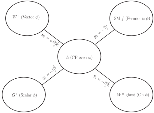
  Figure 1: Schematic representation of the couplings of the Higgs boson and the charged mediators present in the loop for $h\to\gamma\gamma$ as given in Table 5.

  For scalar DM annihilating into photons via the Higgs on the s-channel, we can compute the amplitude by plugging $g_{5}$ in Eq. (60). We find

  $${\cal B}^{h}_{\text{SM}} = \frac{g_{4}\alpha}{\pi v}\left[\underbrace{m_{h}^{2}\left(1-r_{W}^{2}f_{W}\right)}_{\text{loop of $G^{+}$}}\underbrace{-4m_{\text{DM}}\sum_{f}Q_{f}^{2}\,N_{f}\,m_{f}r_{f}\left(1-(r_{f}^{2}-1)f_{f}\right)}_{\text{loop of SM fermions}}\right.$$

  $$\left.+\underbrace{8m_{W}^{2}\left(1-(r_{W}^{2}-2)f_{W}\right)}_{\text{loop of $W^{+}$}}\underbrace{-2m_{W}^{2}\left(1-r_{W}^{2}f_{W}\right)}_{\text{loop of ghosts}}\right]\frac{1}{4m_{\text{DM}}^{2}-m_{h}^{2}+i\Gamma_{h}m_{h}}\,,$$

  where we scale the fermions contribution with their electric charge and number of colors. If we define

  $$A^{h}_{1}(r_{W})=-(2+3r_{W}^{2})-3(2-r_{W}^{2})r_{W}^{2}f_{W} \,, A^{h}_{1/2}(r_{f})=2\,r_{f}^{2}\left(1-(r_{f}^{2}-1)f_{f}\right)\,,$$ (64)

  and notice that $m_{h}^{2}=-(4m_{\text{DM}}^{2}-m_{h}^{2}+i\Gamma_{h}m_{h})+4m_{\text{DM}}^{2}+{\cal O}(\alpha)$, Eq. (• ‣ III.3) can be cast in a more compact form

  $${\cal B}^{h}_{\text{SM}} = -\frac{2m_{\text{DM}}^{2}g_{4}\alpha\left[\sum_{f}Q_{f}^{2}\,N_{f}\,A^{h}_{1/2}(r_{f})+A^{h}_{1}(r_{W})\right]}{\pi v(4m_{\text{DM}}^{2}-m_{h}^{2}+i\Gamma_{h}m_{h})}-\frac{g_{4}\alpha}{\pi v}\left(1-r_{W}^{2}f_{W}\right)\,.$$ (65)

  In the following section, we will see that, in realistic models, the last term typically cancels with another one coming from the amplitude associated to ${\cal L}_{3}$.

  Regarding Majorana DM, the contribution to ${\cal B}$ involving the Higgs in the s-channel is zero, while for vector DM ${\cal B}^{h}_{2}={\cal B}^{h}_{6}=0$ and ${\cal B}^{h}_{1}$ is given by twice ${\cal B}^{h}_{\text{SM}}$ of scalar DM Birkedal et al. (2006).

  Notice that if the CP-even scalar ${\varphi}$ is not the Higgs itself but a neutral particle that mixes with the Higgs and inherits its couplings to the SM particles, we can use the previous expressions for calculating the decay amplitude up to a global factor (obviously, we must also add other possible contributions not present in the SM).

• ${\varphi}$ as the $Z$ boson. For scalar and vector DM, the amplitude vanishes. For Majorana DM, as explained above, the vector boson $Z$ itself does not contribute to the amplitude in the Landau gauge but we have to account for the contribution of its Goldstone boson, $G^{0}$, to the annihilation process. In that case, while ghosts give zero, SM fermions running in the loop give

  $${\cal B}_{\text{SM}}^{Z} = \frac{4\sqrt{2}\,g_{4}\,\alpha\,m_{\text{DM}}^{3}\sum_{f}\pm Q_{f}^{2}\,N_{f}\ r_{f}^{2}f_{f}}{\pi v(4m_{\text{DM}}^{2}-m_{G^{0}}^{2}+i\Gamma_{G^{0}}m_{G^{0}})}=\sqrt{2}\frac{\,g_{4}\alpha m_{\text{DM}}}{\pi v}\,\sum_{f}\pm Q_{f}^{2}N_{f}r_{f}^{2}f_{f}\,,$$ (66)

where we took $g_{5}=\pm m_{f}/v$ with a negative sign for the charged leptons, the down, strange and bottom quarks, and a positive sign for the up, charm and top quarks. In the last equation we used the fact that the Goldstone boson is massless in the Landau gauge.

IV Discussion

IV.1 Summary of the results

Before discussing concrete examples, we would like to summarize our findings. In Section II, we proved that every amplitude form factor can be cast as

$${\cal B} = \sum_{{\phi},{\Phi}}\left(\raisebox{-0.5pt}{\includegraphics[height=34.14322pt]{t1r1}}+\raisebox{-0.5pt}{\includegraphics[height=36.98866pt]{t1r2}}+\raisebox{-0.5pt}{\includegraphics[height=36.98866pt]{t1r3}}+\raisebox{-0.5pt}{\includegraphics[height=36.98866pt]{t3r1}}\right.$$ (67)

$$\underbrace{\left.+\raisebox{-0.5pt}{\includegraphics[height=36.98866pt]{t3r2}}+\raisebox{-0.5pt}{\includegraphics[height=36.98866pt]{t3r5}}+\raisebox{-0.5pt}{\includegraphics[height=36.98866pt]{t3r6}}+\raisebox{-0.5pt}{\includegraphics[height=36.98866pt]{t2r3}}\right)\hskip 60.0pt}_{\text{Contribution of }{\cal L}_{1}\text{ given by Eq.\leavevmode\nobreak\ \eqref{eq:BforL1}}}$$

$$+\underbrace{\sum_{{\Phi}}\left(\raisebox{-0.5pt}{\includegraphics[height=36.98866pt]{t2r2}}+\raisebox{-0.5pt}{\includegraphics[height=39.83368pt]{t3r4}}\right)}_{\text{Contribution of }{\cal L}_{2}\text{ given by Eq.\leavevmode\nobreak\ \eqref{eq:BforL2}}}+\underbrace{\sum_{{\phi}}\left(\raisebox{-0.5pt}{\includegraphics[height=36.98866pt]{t2r1}}+\raisebox{-0.5pt}{\includegraphics[height=36.98866pt]{t3r3}}\right)}_{\text{Contribution of }{\cal L}_{3}\text{ given by Eq.\leavevmode\nobreak\ \eqref{eq:BforL3}}}$$

$$+\underbrace{\sum_{{\varphi},{\phi}}\left(\raisebox{-0.5pt}{\includegraphics[height=36.98866pt]{t4r3}}+\raisebox{-0.5pt}{\includegraphics[height=36.98866pt]{t5r1}}\right)}_{\text{Contribution of }{\cal L}_{4}+{\cal L}_{5}\text{ given by Eq.\leavevmode\nobreak\ \eqref{eq:BforL45}}}+\text{\footnotesize Permutations of the external legs.}$$

Hence, in order to calculate the amplitude and obtain the cross section for DM annihilations into two photons, we have to add the contribution of each interaction. The general algorithm to do this is the following:

1. For spin-1 particles carrying electric charge, use the non-linear Feynman gauge. For the neutral spin-1 bosons, use the Landau gauge.

2. Identify the charged particles that couple directly to DM.

3. If they are charged under $Z_{2}$ (i.e. their type is ${\Phi}$), obtain ${\cal L}_{2}$ and the corresponding coupling $g_{2}$. This gives a contribution to the form factors equal Eq. (31).

4. If the charged particles are $Z_{2}$-even (i.e. their type is ${\phi}$), obtain ${\cal L}_{3}$ and the corresponding coupling $g_{3}$. This gives a contribution to the form factors equal Eq. (42).

5. The interactions ${\cal L}_{1}$ involve two charged mediators directly coupled to DM, one is $Z_{2}$-even and the other one is $Z_{2}$-odd. Extract the couplings $g_{1}$. The corresponding contribution to the form factors is given by Eq. (43).

6. Identify the neutral scalar particles ${\varphi}$ that couple to DM. Obtain ${\cal L}_{4}$ and the corresponding coupling $g_{4}$. Then, determine the charged mediators to which the neutral particle couples to. This gives ${\cal L}_{5}$ and, correspondingly, the coupling $g_{5}$. The total contribution of these particles to the form factors is given by Eqs. (60).

7. After the form factors have been determined, calculate the cross section by means of Eq. (20) for scalar or Majorana DM, or Eq. (24) for vector DM.

We now discuss six different examples in concrete DM models. We will schematically represent the corresponding mediators with figures like Fig. 1. There, each mediator is within in a ellipse that further encloses the couplings associated to vertices where only DM and the mediator are involved (i.e. $g_{2}$, $g_{3}$ or $g_{4}$). In addition, if two different mediators are involved in the same vertex, we join them with a line and write the corresponding coupling on it (i.e. $g_{1}$ or $g_{5}$).

IV.2 Concrete examples

IV.2.1 Wino and Minimal DM

Here we consider fermionic DM that belongs to a self-conjugate $SU(2)_{L}$ multiplet of dimension $N$ with no hypercharge. This sort of scenario includes Wino DM (for $N=3$), or quintuplet Minimal DM ($N=5$). In the first case, a stabilizing symmetry is needed and that is the role of R-parity in the MSSM. In the second case, an accidental symmetry protects the stability of DM at renormalizable level.

Here, the only relevant interaction is given by the vertex ${\cal L}_{1}\propto$ DM DM${}^{+}W^{-}$, where DM⁺ is the fermion in the multiplet with charge $+e$. The mediators and the corresponding couplings are shown in Fig. 2.

Figure 2: Schematic representation of the mediators and the couplings for Wino and Minimal DM.

Note that if no radiative correction is taken into account, we have $m_{\text{DM}^{+}}=m_{\text{DM}}$, i.e. $r_{\text{DM}^{+}}=1$. Plugging this and the couplings of Fig. 2 in Eqs. (102), we can calculate the coefficients in front of the Passarino–Veltman functions for the form factor of Eq. (43). The corresponding cross section is

$$\sigma v=\bigg{|} \dfrac{r_{W}^{4}+2r_{W}^{2}-4}{(1-r_{W}^{2})(2-r_{W}^{2})}C_{0}(0,1,-1,r_{W}^{2},r_{W}^{2},1)+\dfrac{r_{W}^{2}-2}{r_{W}^{2}\left(-1+r_{W}^{2}\right)}C_{0}(0,1,-1,1,1,r_{W}^{2})$$

$$-4\left(\frac{r_{W}^{2}-1}{r_{W}^{2}-2}\right)\,\,C_{0}\left(0,4,0,r_{W}^{2},r_{W}^{2},r_{W}^{2}\right)-\frac{2}{r_{W}^{2}}\,\,C_{0}\left(0,4,0,1,1,1\right)\bigg{|}^{2}\dfrac{\alpha^{4}(N^{2}-1)^{2}}{16\pi s_{W}^{4}m_{\text{DM}}^{2}}\,.$$ (68)

For the Wino case, this equation agrees explicitly with Eq. (22) of Ref. Bern et al. (1997). Even though it can be simplified further in terms of dilogarithms, for the sake of illustration, we will only recast the cross section in the limit $m_{\text{DM}}\gg m_{W}$, that is, when $r_{W}\to 0$. To that end, notice that in that limit, each of Passarino–Veltman functions diverges at most logarithmically. Notice also that the coefficient in front of $C_{0}(0,1,-1,r_{W}^{2},r_{W}^{2},1)$ and $C_{0}\left(0,4\,,0,r_{W}^{2},r_{W}^{2},r_{W}^{2}\right)$ are finite in that limit, whereas those in front of $C_{0}(0,1,-1,1,1,r_{W}^{2})$ and $C_{0}\left(0,4,0,1,1,1\right)$ diverge like $1/r_{W}^{2}$. Hence, the latter Passarino–Veltman functions dominate the cross section in that limit. They give Patel (2015)

$$C_{0}\left(0,1,-1,1,1,r_{W}^{2}\right) \simeq-\frac{\pi^{2}}{8}+\frac{\pi r_{W}}{2}+{\cal O}(r_{W}^{2})\,, C_{0}\left(0,4,0,1,1,1\right) =-\frac{\pi^{2}}{8}\,.$$ (69)

Using this, we find $\sigma v=\pi\alpha^{4}(N^{2}-1)^{2}/16m_{W}^{2}s_{W}^{4}$, in agreement with Refs. Bergstrom and Ullio (1997); Cirelli et al. (2006). The same expression can also be obtained by calculating the Sommerfeld effect in the limit in which the potential is perturbative Hisano et al. (2007); Garcia-Cely et al. (2015).

IV.2.2 Scotogenic DM

In this scenario Ma (2006); Kubo et al. (2006), there two types of fields charged under the $Z_{2}$ symmetry: a scalar $H^{\prime}=(H^{+},\frac{1}{\sqrt{2}}(H^{0}+iA^{0}))^{T}$ with the same quantum numbers of the SM scalar doublet $H$, and a handful of right-handed neutrinos $N_{j}$. The interactions of the scalar doublets are described by

$$\mathcal{L}= \left(D_{\mu}H\right)^{\dagger}\left(D^{\mu}H\right)+\left(D_{\mu}H^{\prime}\right)^{\dagger}\left(D^{\mu}H^{\prime}\right)-\mu_{1}^{2}|H|^{2}-\mu_{2}^{2}|H^{\prime}|^{2}$$

$$- \lambda_{1}|H|^{4}-\lambda_{2}|H^{\prime}|^{4}-\lambda_{3}|H|^{2}|H^{\prime}|^{2}-\lambda_{4}|H^{\dagger}H^{\prime}|^{2}-\frac{\lambda_{5}}{2}\left[\left(H^{\dagger}H^{\prime}\right)^{2}+\text{h.c.}\right]\,.$$ (70)

For the right-handed neutrinos, the relevant interactions are with the SM lepton doublets $L_{\beta}$, which are given by

$${\cal L}=\epsilon_{ab}h_{\beta j}\overline{N_{j}}P_{L}L^{a}_{\beta}H^{\prime b}\,.$$ (71)

The DM candidate is the lightest particle with $Z_{2}$ charge. If such particle is one of the right-handed neutrinos, DM can annihilate into photons by means of one-loop diagrams containing a SM charged lepton and $H^{+}$. The corresponding couplings are shown in Fig. 3, where DM was taken as $N_{1}$. Notice that there are no s-channel mediators. Now, it is straightforward to calculate ${\cal B}$ by means of Eqs. (• ‣ C) and (43). The resulting cross section is

$$\sigma v = \frac{\alpha^{2}}{64\pi^{3}m_{1}^{2}}\sum_{\beta}\frac{r_{H}^{4}h_{\beta 1}^{4}}{\left(r_{e_{\beta}}^{2}-r_{H}^{2}-1\right)^{2}\left(r_{e_{\beta}}^{2}-r_{H}^{2}\right)^{2}}\bigg{|}\frac{r_{e_{\beta}}^{2}}{r_{H}^{2}}\left(1+r_{e_{\beta}}^{2}-r_{H}^{2}\right)C_{0}(0,1,-1,r_{e_{\beta}}^{2},r_{e_{\beta}}^{2},r_{H}^{2})$$ (72)

$$-(1-r_{e_{\beta}}^{2}+r_{H}^{2})C_{0}(0,1,-1,r_{H}^{2},r_{H}^{2},r_{e_{\beta}}^{2})+\frac{2\,r_{e_{\beta}}^{2}(r_{H}^{2}-r_{e_{\beta}}^{2})}{r_{H}^{2}}C_{0}(0,4,0,r_{e_{\beta}^{2}},r_{e_{\beta}}^{2},r_{e_{\beta}}^{2})\bigg{|}^{2}.$$

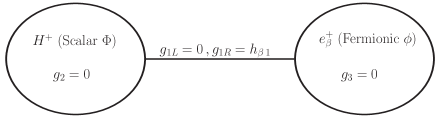
Figure 3: Schematic representation of the mediators and the couplings for Scotogenic DM.

In the limit of $m_{\text{DM}}\gg m_{e_{\beta}^{+}}$, i.e. when $r_{e_{\beta}}\to 0$, this expression gives (e.g. Ref. Garny et al. (2015))

$$\sigma v= \frac{\alpha^{2}h^{4}_{\beta 1}}{256\pi^{3}m_{1}^{2}}|2\,C_{0}(0,1,-1,r_{H}^{2},r_{H}^{2},0)|^{2}=\frac{\alpha^{2}h^{4}_{\beta 1}}{256\pi^{3}m_{1}^{2}}\left|\text{Li}_{2}\left(\frac{1}{r_{H}^{2}}\right)-\text{Li}_{2}\left(-\frac{1}{r_{H}^{2}}\right)\right|^{2}\,,$$ (73)

IV.2.3 Singlet scalar DM

Suppose that DM is a scalar field $\phi$, which is singlet under $SU(2)_{L}$ Silveira and Zee (1985); McDonald (1994). Then, the only non-trivial interaction of DM with the SM takes place via the so-called Higgs portal ${\cal L}=\lambda_{H}\,\text{DM}^{2}H^{\dagger}H\supset\lambda_{H}\text{DM}^{2}(G^{+}G^{-}+v\,h)$. Hence, there are five mediators, which are shown in Fig. 4. First, we have $G^{+}$, which is involved in the ${\cal L}_{3}$ interaction. The corresponding contribution to the form factor can be computed with Eq. (42). Second, we have the Higgs boson, which acts as mediator on the s-channel. The contribution of the Higgs boson was already calculated and reported in Eq. (65). The total form factor is

$${\cal B} = \frac{\alpha\lambda_{H}}{\pi}\left(1-r_{W}^{2}f_{W}\right)+{\cal B}^{h}_{\text{SM}}$$ (74)

$$= -\dfrac{2m_{\text{DM}}^{2}\alpha\,\lambda_{H}}{\pi\left(4m_{\text{DM}}^{2}-m_{h}^{2}+i\Gamma_{h}m_{h}\right)}\left(\sum_{f}N_{f}Q_{f}^{2}A^{h}_{1/2}(r_{f})+A^{h}_{1}(r_{W})\right)\,,$$

which, according to Eq. (20), corresponds to a cross section

$$\sigma v=\dfrac{m_{\text{DM}}^{2}\alpha^{2}\,\lambda_{H}^{2}}{8\pi^{3}\left((4m_{\text{DM}}^{2}-m_{h}^{2})^{2}+m_{h}^{2}\Gamma_{h}^{2}\right)}\bigg{|}\sum_{f}Q_{f}^{2}\,N_{f}\,A^{h}_{1/2}(r_{f})+A^{h}(r_{W})\bigg{|}^{2}\,.$$ (75)

This expression is in agreement with the results of the literature (see e.g. Duerr et al. (2016b); Gunion et al. (2000)).

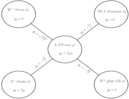
Figure 4: Schematic representation of the mediators and the couplings for singlet scalar DM.

IV.2.4 Inert Higgs DM

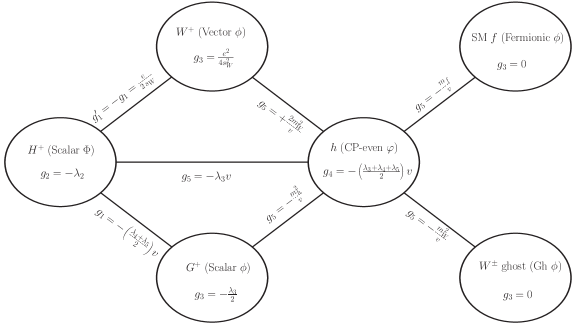
Figure 5: Schematic representation of the mediators and the couplings for inert Higgs DM.

Suppose that we have an additional scalar doublet $H^{\prime}$ which is charged under a $Z_{2}$ symmetry (like the Scotogenic model above, but without right-handed neutrinos). Hence, the relevant interactions are described by Eq. (70) and the DM candidate is the lightest particle that is charged under $Z_{2}$. Without loss of generality, we assume this is the $H^{0}$ boson.

In this case, the calculation of the cross section is significantly more difficult than in the previous examples. First, we have diagrams with the Higgs on the s-channel, receiving contributions not only from SM particles (computed already in Eq. (• ‣ III.3)) but also from the additional scalar $H^{+}$. Second, and more importantly, the direct interactions of DM with charged mediators -which give rise to diagrams with topologies 1, 2 and 3- are of two kinds. One of them is of scalar nature, in which the mediators are scalars $H^{+}$ and $G^{+}$; the other one is associated to the gauge interaction, whose charged mediators are $H^{+}$ again and the $W^{+}$ boson. All this is schematically represented in Fig. 5.

The contribution of ${\cal L}_{2}$ and ${\cal L}_{3}$ to the form factor is given by Eqs. (31) and (42)

$$B\bigg{|}_{{\cal L}_{2}+{\cal L}_{3}}=\underbrace{-\frac{\alpha\lambda_{2}}{\pi}\left(1-r_{H}^{2}f_{H}\right)}_{\text{Loop of }H^{+}}\underbrace{-\frac{\alpha\lambda_{3}}{2\pi}\left(1-r_{W}^{2}f_{W}\right)}_{\text{Loop of }G^{+}}\underbrace{-\frac{4\pi\alpha^{2}}{s_{W}^{2}}\left(1-(r_{W}^{2}-2)f_{W}\right)}_{\text{Loop of }W^{+}}\,.$$ (76)

For the Higgs on the s-channel, we can use Eq. (65) for the SM piece and add, by means of Eq. (60), the contribution associated to the additional charged particle. This is

$${\cal B}^{h} = {\cal B}^{h}_{\text{SM }}-\dfrac{\alpha\lambda_{3}\lambda_{h}v^{2}}{\pi\left(4-r_{h}^{2}+ir_{h}\Gamma_{h}/m_{H^{0}}\right)}\left(1-r_{H}^{2}f_{H}\right)$$

$$= \left(\dfrac{2\pi\alpha\left(\sum_{f}N_{f}Q_{f}^{2}A^{h}_{1/2}(r_{f})+A^{h}_{1}(r_{W})\right)-s_{W}^{2}r_{W}^{2}\lambda_{3}(1-r_{H}^{2}f_{H})}{\pi^{2}\left(4-r_{h}^{2}+ir_{h}\Gamma_{h}/m_{H^{0}}\right)}+\frac{\alpha\left(1-r_{W}^{2}f_{W}\right)}{\pi}\right)\lambda_{h}\,,$$

with

$$\lambda_{h}=\frac{1}{2}\left(\lambda_{3}+\lambda_{4}+\lambda_{5}\right)=\frac{\lambda_{3}}{2}-\frac{\pi\alpha(r_{H}^{2}-1)}{s_{W}^{2}r_{W}^{2}}\,.$$ (78)

In the last line, we use $m_{W}=e\,v/2s_{W}$, and the fact that, after electroweak symmetry breaking, the charged particle in the doublet and the DM candidate are not longer degenerate in mass. Indeed, $m_{H^{+}}^{2}=m_{H^{0}}^{2}-(\lambda_{4}+\lambda_{5})v^{2}/2$. This shows that even though there are many masses and parameters, the form factor ${\cal B}$ depends only on four unknown variables: $r_{W},r_{H},\lambda_{2}$ and $\lambda_{3}$. Notice that the first one is just the inverse of the DM mass in units of $m_{W}$. Using this, we can calculate the contribution of ${\cal L}_{1}$ by means of Eq. (43), with the corresponding coefficients extracted from Eqs. (98) and (100).

Finally, putting everything together, we obtain

$$\sigma v= \Bigg{|}\frac{r_{H}^{2}+3r_{W}^{2}-1}{r_{W}^{2}}+\frac{\tilde{\lambda}_{2}s_{W}^{2}}{\pi\alpha}\left(1-r_{H}^{2}f_{H}\right)-\frac{2\lambda_{h}s_{W}^{2}}{\pi\alpha}\left(\dfrac{\sum_{f}N_{f}Q_{f}^{2}A^{h}_{1/2}(r_{f})+A^{h}_{1}(r_{W})}{4-r_{h}^{2}+ir_{h}\Gamma_{h}/m_{H^{0}}}\right)$$

$$+\left(6-3r_{W}^{2}+\frac{4r_{W}^{2}-4}{1+r_{H}^{2}-r_{W}^{2}}\right)f_{W}+\left(5-r_{H}^{2}+\frac{4r_{H}^{2}-4}{1+r_{W}^{2}-r_{H}^{2}}\right)\frac{r_{H}^{2}f_{H}}{r_{W}^{2}}$$

$$-2\left(1+\frac{5r_{H}^{2}-r_{W}^{2}+1}{(r_{H}^{2}-r_{W}^{2})(1+r_{H}^{2}-r_{W}^{2})}\right)C_{0}(0,1,-1,r_{W}^{2},r_{W}^{2},r_{H}^{2})$$

$$-\frac{2r_{H}^{2}}{r_{W}^{2}}\left(1+\frac{5r_{W}^{2}-r_{H}^{2}+1}{(r_{W}^{2}-r_{H}^{2})(1+r_{W}^{2}-r_{H}^{2})}\right)C_{0}(0,1,-1,r_{H}^{2},r_{H}^{2},r_{W}^{2})\Bigg{|}^{2}\frac{\alpha^{4}}{32\pi s_{W}^{4}m_{H^{0}}^{2}},$$ (79)

with

$$\tilde{\lambda}_{2}=\lambda_{2}+\dfrac{s_{W}^{2}r_{W}^{2}\lambda_{3}\lambda_{h}}{\pi\alpha\left(4-r_{h}^{2}+ir_{h}\Gamma_{h}/m_{H^{0}}\right)}\,.$$ (80)

This result agrees with those of Refs. Gustafsson et al. (2007); Garcia Cely (2014-08-06), which were found numerically but not analytically. It also agrees with the cross section obtained with the Sommerfeld effect in the limit of perturbative potential Garcia-Cely et al. (2016).

IV.2.5 Singlet-doublet DM and Higgsinos

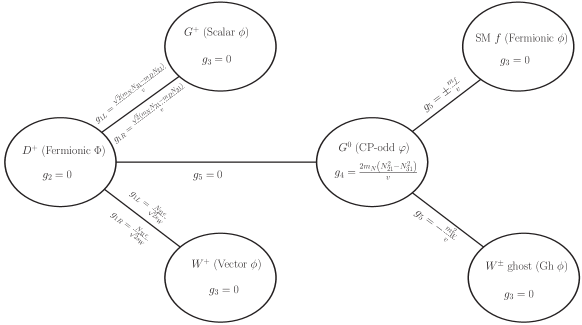
Figure 6: Schematic representation of the mediators and the couplings for singlet-doublet DM.

In this case, the fields that are charged under $Z_{2}$ are all chiral fermions, two of them which are $SU(2)_{L}$-doublets with hypercharge $\pm 1/2$ and one gauge singlet. After electroweak symmetry breaking, one charged fermion $D^{+}$ is obtained along with three Majorana particles. The lightest of the latter is the DM candidate, which we call $N$. The reader can find more details of the model and its phenomenology in Refs.D’Eramo (2007); Abe et al. (2014); Calibbi et al. (2015); Restrepo et al. (2015). Here just mention that this DM candidate interacts with the SM gauge bosons (and its Goldstone bosons) by means of

$${\cal L} = \frac{2m_{N}}{v}\left(N_{21}^{2}-N_{31}^{2}\right)G^{0}\overline{N}\gamma_{5}N+\left(\dfrac{e}{2s_{W}}\overline{N}\not{W}^{+}(N_{21}P_{L}+N_{31}P_{R})D^{-}\right.$$ (81)

$$\left.+\frac{\sqrt{2}}{v}G^{+}\overline{N}\left((m_{N}N_{31}-m_{D}N_{21})P_{L}+(m_{N}N_{21}-m_{D}N_{31}\right)P_{R})D^{-}+\text{h.c.}\right)\,.$$

where $N_{21}$ and $N_{31}$ are mixing parameters. Higgsino DM is a particular realization of this scenario when such parameters take specific values and the $Z_{2}$ symmetry corresponds to R-parity. Furthermore, the pure Higgsino limit is the situation for which $N_{21}=N_{31}=1/\sqrt{2}$ and the charged particle and the DM have the same mass, i.e. $m_{D}=m_{N}$. Notice that we omit the coupling to $Z$ boson, as it is not relevant in the Landau gauge. Also, note that the $D^{+}$ does not interact with the Goldstone boson, $G^{0}$. Such interaction is not renormalizable because it requires at least two scalar doublets and two fermionic doublets.

The calculation of the annihilation cross section is similar to that of the inert doublet model. First, we have diagrams with the $Z$ on the s-channel, which nevertheless only receive contributions from the SM fields (see Fig 6). Hence, we can use Eq. (66) directly. Second, interactions of DM with charged mediators -which give rise interactions type ${\cal L}_{1}$- are between $D^{+}$ and $G^{+}$ or $W^{+}$. All this is summarized in Fig. 6.

With those couplings, we can use Eqs. (• ‣ C) and (102) to determine the coefficients in front of Passarino–Veltman functions in Eq. (43). The final result is

$$\sigma v = \frac{\alpha^{4}(N_{21}^{2}+N_{31}^{2})^{2}}{16\pi s_{W}^{4}m_{\text{DM}}^{2}}\Bigg{|}\frac{(N_{21}^{2}-N_{31}^{2})\sum_{f}\left(\pm Q_{f}^{2}N_{f}r_{f}^{2}f_{f}\right)}{r_{W}^{2}(N_{21}^{2}+N_{31}^{2})}\,$$ (82)

$$+\left(\frac{2r_{W}^{4}-r_{W}^{2}\left(r_{D}^{2}+1\right)-r_{D}^{4}+6r_{D}^{2}-1}{\left(r_{W}^{2}-r_{D}^{2}-1\right)\left(r_{W}^{2}-r_{D}^{2}\right)}+\frac{12yr_{D}}{r_{W}^{2}-r_{D}^{2}}\right)C_{0}(0,1,-1,r_{W}^{2},r_{W}^{2},r_{D}^{2})$$

$$-\frac{r_{D}^{2}\left(-2r_{W}^{4}+r_{W}^{2}\left(r_{D}^{2}-3\right)+\left(r_{D}^{2}-1\right)^{2}\right)+12yr_{D}r_{W}^{2}}{r_{W}^{2}\left(r_{W}^{2}-r_{D}^{2}\right)\left(r_{W}^{2}-r_{D}^{2}+1\right)}C_{0}(0,1,-1,r_{D}^{2},r_{D}^{2},r_{W}^{2})$$

$$+\frac{4\left(r_{W}^{2}-1\right)}{r_{W}^{2}-r_{D}^{2}-1}f_{W}-\frac{r_{D}\left(r_{D}\left(2r_{W}^{2}-r_{D}^{2}+1\right)+y\left(-8r_{W}^{2}+2r_{D}^{2}-2\right)\right)}{r_{W}^{2}\left(r_{W}^{2}-r_{D}^{2}+1\right)}f_{D}\Bigg{|}^{2}\,,$$

with $y=N_{21}\,N_{31}/(N_{21}^{2}+N_{31}^{2})$. The pure Higgsino limit, when $m_{N}\gg m_{W}$, gives $\sigma v=\pi\alpha^{4}/4m_{W}^{2}s_{W}^{4}$ in agreement with Ref. Rudaz (1989); Bern et al. (1997).

IV.2.6 Vector Kaluza-Klein DM

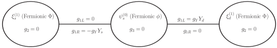
Figure 7: Schematic representation of the mediators and the couplings for Kaluza-Klein DM.

The annihilation of the Kaluza-Klein (KK) DM particle $B^{(1)}$ into two photons was analyzed in the Ref. Bergstrom et al. (2005). This is a nice example of vector DM where the $Z_{2}$ symmetry corresponds to the KK parity (indicated as superscript). The particle content of this model consists of a zero level KK fermion $\psi^{(0)}$ as well as of $\xi_{s}^{(1)}$ and $\xi_{d}^{(1)}$, which are its first singlet and doublet excitation with hypercharge $Y_{s}$ and $Y_{d}$, respectively. The DM particle couples to the other fermions according to the Lagrangian

$$\mathcal{L}^{{}^{\prime}}=-g_{Y}Y_{s}B_{\mu}^{(1)}\bar{\xi}_{s}^{(1)}\gamma^{\mu}P_{R}\psi^{(0)}+g_{Y}Y_{d}B_{\mu}^{(1)}\bar{\xi}_{d}^{(1)}\gamma^{\mu}P_{L}\psi^{(0)}+\text{h.c.}\,,$$ (83)

which gives rise to the mediator classification of Fig. 7. Only interactions type ${\cal L}_{1}$ are present. Using Eqs. (126),(133) and (140) we can calculate the form factors ${\cal B}_{1}$, ${\cal B}_{2}$ and ${\cal B}_{6}$, respectively. Moreover, we can compute the corresponding cross section by means of Eq. (24). This calculation was previously performed in Ref. Bergstrom et al. (2005) for the case when the zero-level KK excitation $\psi^{(0)}$ is massless. Our results, valid for arbitrary masses, are in agreement with the expressions reported in that paper in the limit $m_{\psi}\to 0$.

V Conclusions

Gamma-ray lines produced in WIMP annihilations play a significant role for indirect DM searches because they stand out of the soft featureless background and no astrophysical process is known to produce them. A model-independent study of gamma-ray lines is nevertheless challenging because the calculation of the corresponding cross sections crucially depend on multiple details of the underlying DM model. This work is a step towards such study.

By means of a careful classification of the one-loop diagrams leading to DM annihilation into two photons, we have shown that for any model satisfying conditions (i)-(v), the annihilation amplitude - and consequently, the cross section- can be calculated by just adding different expressions that we report in Eq. (67). Our results were summarized and exemplified in Sec. IV. We also provide a Mathematica notebook where this is done . We find an agreement with previous works done in the context of popular DM models.

A natural extension of this article is applying the same methods for calculating the annihilation cross sections associated to the final states $Z\gamma$ and $h\gamma$. In addition, one can consider going beyond the conditions (i)-(v), for instance by calculating the annihilation cross section into two photons for Dirac or complex scalar DM. We leave this for a future work.

Appendix A Gauge choice for vector boson mediators

A.1 Charged gauge bosons

In order to calculate the annihilation amplitude, we assume that the underlying model meets conditions (i)-(v). The third one in particular is not satisfied by $W^{+}$ boson in ordinary $R_{\xi}$ gauges, because of the presence of the interaction

$$\delta{\cal L}=eM_{W}\,G^{+}W^{-\mu}A_{\mu}+\text{h.c.}\,$$ (84)

The solution to this problem is to work in a different gauge. The gauge fixing term in the ordinary Feynman gauge is given by ${\cal L}_{\text{gf}}=-f^{*}f$ with $f=\partial_{\mu}W^{+\mu}-im_{W}G^{+}$ . If we work instead with $f=\partial_{\mu}W^{+\mu}-im_{W}G^{+}+ieA_{\mu}W^{+\mu}$, we clearly cancel the interaction term in Eq. (84). In fact, this procedure replaces such term by the following interactions between the $W$ bosons and the photons

$$\delta{\cal L}=-e^{2}A^{\mu}A^{\nu}W^{-}_{\mu}W^{+}_{\nu}+ieA^{\mu}(W^{+}_{\mu}\partial^{\nu}W^{-}_{\nu}-W^{-}_{\mu}\partial^{\nu}W^{+}_{\nu})\,.$$ (85)

This is the so-called Feynman non-linear gauge. The new gauge fixing term gives rise to the following interactions between the Faddeev–Popov ghosts associated to the $W^{\pm}$ boson and photons Pasukonis (2007)

$${\cal L}=-ieA_{\mu}\left(\partial_{\mu}\overline{c}^{-}c^{+}-\partial_{\mu}\overline{c}^{+}c^{-}\right)\underbrace{-ieA_{\mu}\left(\overline{c}^{+}\partial_{\mu}c^{-}-\overline{c}^{-}\partial_{\mu}c^{+}\right)-e^{2}A_{\mu}A^{\mu}\left(\overline{c}^{-}c^{+}+\overline{c}^{+}c^{-}\right)}_{\text{only present in the Feynman non-linear gauge}}\,.$$ (86)

Even though the expressions reported here are those associated to the $W$ boson, they can be generalized to any charged gauge boson by rescaling the electric charge. Because of that, for arbitrary vector charged mediators ${\phi}$, we assume that terms like Eq. (84) are not present, and include Eq. (85) to their interactions with photons. Furthermore, we describe the corresponding ghosts by means of Eq. (86).

A.2 Neutral gauge bosons in the s-channel

In this appendix, we show that when DM annihilates into two photons via a massive gauge boson in the s-channel, the corresponding amplitude can be calculated by considering only the associated Goldstone boson in the Landau gauge. This has been used in Ref. Moretti (2015) in order to calculate the contribution of the process $q\overline{q}\to Z^{*}\to\gamma\gamma$ to the SM background for a diphoton signal. Here we generalize their arguments to an arbitrary neutral gauge boson and apply them to DM annihilations.

Let us start by considering the off-shell decay of a vector particle into two photons ${\varphi}^{\rho}(k)\to\gamma^{\mu}(q)\gamma^{\nu}(q^{\prime})$. After stripping the polarization vectors, the most general decay amplitude, compatible with Bose statistics and Lorentz invariance, is given by

$${\cal M}^{\rho\mu\nu}= C_{1}\,(q^{\nu}g^{\mu\rho}+q^{\prime\mu}g^{\nu\rho})+C_{2}\,k^{\rho}g^{\mu\nu}+C_{3}\,k^{\rho}q^{\nu}q^{\prime\mu}$$

$$+ C_{4}\,\epsilon^{\rho\mu\nu\alpha}(q-q^{\prime})_{\alpha}+\left(C_{5}k^{\rho}{\epsilon}^{\mu\nu\alpha\beta}+C_{6}(q^{\nu}{\epsilon}^{\mu\rho\alpha\beta}-q^{\prime\mu}{\epsilon}^{\nu\rho\alpha\beta})\,q_{\alpha}q^{\prime}_{\beta}\right)\,,$$ (87)

where $C_{i}$ are scalar functions. This expression can be simplified further in the center-of-mass frame. First, there the photons move with opposite three-momentum and consequently their polarization vectors not only satisfy $q\cdot\epsilon=0$ and $q^{\prime}\cdot\epsilon^{\prime}=0$ but also $q^{\prime}\cdot\epsilon=0$ and $q\cdot\epsilon^{\prime}=0$. This makes $C_{1}$, $C_{3}$ and $C_{6}$ irrelevant once $M^{\rho\mu\nu}$ is contracted with the polarization vectors. In addition, for the same reason, $\{k,q-q^{\prime},\epsilon,\epsilon^{\prime}\}$ is an orthogonal basis in the center-of-mass frame, which can be used to prove that $\epsilon^{\rho\mu\nu\alpha}\epsilon^{*}_{\mu}\epsilon^{\prime*}_{\nu}(q-q^{\prime})_{\alpha}=-k^{\rho}{\epsilon}^{\mu\nu\alpha\beta}\epsilon^{*}_{\mu}\epsilon^{\prime*}_{\nu}q_{\alpha}q^{\prime}_{\beta}/q\cdot q^{\prime}$, and consequently that $C_{4}$ can be absorbed into $C_{5}$. We conclude that the amplitude is determined by

$${\cal M}^{\rho\mu\nu}= k^{\rho}\left(C_{2}\,g^{\mu\nu}+C_{5}{\epsilon}^{\mu\nu\alpha\beta}\,q_{\alpha}q^{\prime}_{\beta}\right)\,.$$ (88)

This is just a restatement of the Landau–Yang theorem Landau (1948); Yang (1950). If the gauge boson is on its mass-shell, its polarization vector $\epsilon(k)$ satisfies $k\cdot\epsilon(k)=0$ and, according to the previous equation, the decay amplitude vanishes. Furthermore, on an arbitrary $R_{\xi}$ gauge (linear or not), the amplitude for the process $\text{DM}\text{DM}\to{\varphi}^{*}\to\gamma\gamma$ is proportional to

$$\left(g_{\sigma\rho}+\frac{(\xi-1)k_{\sigma}k_{\rho}}{k^{2}-\xi m_{\varphi}^{2}}\right)M^{\rho\mu\nu}\epsilon^{*}_{\mu}\epsilon^{\prime*}_{\nu}=\xi\,k_{\sigma}\frac{\left(k^{2}-m_{\varphi}^{2}\right)\left(C_{2}\,g^{\mu\nu}+C_{5}{\epsilon}^{\mu\nu\alpha\beta}\,q_{\alpha}q^{\prime}_{\beta}\right)\epsilon^{*}_{\mu}\epsilon^{\prime*}_{\nu}}{k^{2}-\xi m_{\varphi}^{2}}\,.$$ (89)

When the vector particle is on-shell, this expression vanishes as expected from the Landau–Yang theorem. Most importantly, in the Landau gauge, $\xi=0$, the expression vanishes even off-shell. The decay of the gauge bosons into two photons is thus given only by the Goldstone boson contribution. Since the latter is a massless scalar, we can calculate the annihilation amplitude by applying the results presented in Sec. III.3.

Appendix B Reduction of tensor integrals in the non-relativistic limit

Box diagrams in the annihilation amplitude such as

$$\raisebox{-0.5pt}{\includegraphics[height=42.67912pt]{t1r1}}+\raisebox{-0.5pt}{\includegraphics[height=42.67912pt]{t1r2}}+\raisebox{-0.5pt}{\includegraphics[height=42.67912pt]{t1r3}}$$ (90)

lead to the next four-point loop integrals Passarino and Veltman (1979)

$$D_{0}; D_{\mu};D_{\mu\nu};D_{\mu\nu\rho};D_{\mu\nu\rho\sigma}\left(k_{1}^{2},(k_{2}-k_{1})^{2},(k_{3}-k_{2})^{2},(k_{4}-k_{3})^{2},k_{2}^{2},(k_{3}-k_{1})^{2},m_{1}^{2},m_{2}^{2},m_{3}^{2},m_{4}^{2}\right)$$

$$=\int\frac{d^{D}l}{i\pi^{2}}\dfrac{1;l_{\mu};l_{\mu}l_{\nu};l_{\mu}l_{\nu}l_{\rho};l_{\mu}l_{\nu}l_{\rho}l_{\sigma}}{[l^{2}-m_{1}^{2}][(l+k_{1})^{2}-m_{2}^{2}][(l+k_{2})^{2}-m_{3}^{2}][(l+k_{3})^{2}-m_{4}^{2}]}$$ (91)

$$=D_{0};D_{\mu};D_{\mu\nu};D_{\mu\nu\rho};D_{\mu\nu\rho\sigma}\left(1,2,3,4\right)\,,$$ (92)

where the $k_{N}$ are related to the external momenta $p_{i}$ as $k_{N}=\sum_{i=1}^{N}p_{i}$. In the original Passarino–Veltman schema, it is possible to reduce the four-point tensor integrals to scalar expressions. However, such procedure is based on the assumption of independent external momenta $p_{i}$, which is not our case because the DM legs have the same momentum $(m_{\text{DM}},0,0,0)$ in the non-relativistic limit. Nevertheless, since there are three independent momenta, we can still reduce the tensor four-point integrals to a linear combination of tensor three-point integrals, which can be reduced to scalar functions. For this, we closely follow the algebraic reduction of Refs. Stuart (1988); Stuart and Gongora (1990); Stuart (1995), but expanding Eq. (B) in terms of the momenta $k_{i}$ instead of the external momenta $p_{i}$.

As an example, we consider the scalar reduction of the tensor $D_{\mu}$. Very schematically, we have

$$D_{\mu} =\int\dfrac{d^{D}l}{i\pi^{2}}\dfrac{l_{\mu}}{[l^{2}-m_{1}^{2}][(l+k_{1})^{2}-m_{2}^{2}][(l+k_{2})^{2}-m_{3}^{2}][(l+k_{3})^{2}-m_{4}^{2}]}=\int\frac{d^{D}l}{i\pi^{2}}\dfrac{l_{\mu}}{[1][2][3][4]}$$

$$= \alpha_{123}\int\frac{d^{D}l}{i\pi^{2}}\dfrac{l_{\mu}}{[1][2][3]}+\alpha_{124}\int\frac{d^{D}l}{i\pi^{2}}\dfrac{l_{\mu}}{[1][2][4]}+\alpha_{134}\int\frac{d^{D}l}{i\pi^{2}}\dfrac{l_{\mu}}{[1][3][4]}+\alpha_{234}\int\frac{d^{D}l}{i\pi^{2}}\dfrac{l_{\mu}}{[2][3][4]}$$

$$= \alpha_{123}C_{\mu}(1,2,3)+\alpha_{124}C_{\mu}(1,2,4)+\alpha_{134}C_{\mu}(1,3,4)+\alpha_{234}\left(C_{\mu}(2,3,4)-k_{1\mu}C_{0}(2,3,4)\right)\,,$$ (93)

where we did the substitution $l+k_{1}\rightarrow l^{{}^{\prime}}$ in the last integral to cast it in the canonical form of a three-point function. Also, the coefficients $\alpha_{ijk}$ can be obtained by solving the system Stuart (1988)

$$\begin{pmatrix}1&1&1&1\\ 0&p_{1}^{2}&(p_{1}^{2}-p_{2}^{2}+p_{5}^{2})/2&(p_{1}^{2}+p_{4}^{2}-p_{6}^{2})/2\\ 0&(-p_{1}^{2}-p_{2}^{2}+p_{5}^{2})/2&(-p_{1}^{2}+p_{2}^{2}+p_{5}^{2})/2&(-p_{1}^{2}-p_{3}^{3}+p_{5}^{2}+p_{6}^{2})/2\\ -m_{1}^{2}&p_{1}^{2}-m_{2}^{2}&p_{5}^{2}-m_{3}^{2}&p_{4}^{2}-m_{4}^{2}\end{pmatrix}\begin{pmatrix}\alpha_{234}\\ \alpha_{134}\\ \alpha_{124}\\ \alpha_{123}\end{pmatrix}=\begin{pmatrix}0\\ 0\\ 0\\ 1\end{pmatrix}\,,$$ (94)

with $p_{5}=p_{1}+p_{2}$ and $p_{6}=p_{2}+p_{3}$ . The three-point tensor integrals can now be reduced to scalar integrals

$$D_{\mu}= \alpha_{123}\left(k_{1\mu}C_{1}(1,2,3)+k_{2\mu}C_{2}(1,2,3)\right)+\alpha_{124}\left(k_{1\mu}C_{1}(1,2,4)+k_{3\mu}C_{2}(1,2,4)\right)$$

$$+\alpha_{134}\left(k_{2\mu}C_{1}(1,3,4)+k_{3\mu}C_{2}(1,3,4)\right)$$

$$+\alpha_{234}\left((k_{2\mu}-k_{1\mu})C_{1}(2,3,4)+(k_{3\mu}-k_{1\mu})C_{2}(2,3,4)-k_{1\mu}C_{0}(2,3,4)\right)\,.$$ (95)

This expression must be compared against the defining expression for the scalar functions $D_{\mu}=k_{1\mu}D_{1}+k_{2\mu}D_{2}+k_{3\mu}D_{3}$, which leads to

$$D_{1}= \,\alpha_{123}C_{1}+\alpha_{124}C_{1}-\alpha_{234}\left(C_{0}+C_{1}+C_{2}\right)$$

$$D_{2}= \,\alpha_{123}C_{2}+\alpha_{134}C_{1}+\alpha_{234}C_{1}$$

$$D_{3}= \,\alpha_{124}C_{2}+\alpha_{134}C_{2}+\alpha_{234}C_{2}\,,$$ (96)

with $\alpha_{ijk}C_{l}\equiv\alpha_{ijk}C_{l}(i,j,k)$. A similar reduction can be applied to the scalar integral $D_{0}$, which gives rise to

$$D_{0}= \,\alpha_{123}C_{0}+\alpha_{124}C_{0}+\alpha_{134}C_{0}+\alpha_{234}C_{0}\,.$$ (97)

Appendix C Coefficients in the Passarino–Veltman reduction of the amplitudes

This appendix reports the coefficients in Eq. (43) according to the spin of the particles involved in the one-loop diagram.

Scalar DM

For the scalar case we always find $x_{6}=x_{7}=x_{8}=0$. The non-zero coefficients for each mediator combination are:

• Scalar ${\Phi}$ and scalar ${\phi}$

  $$x_{1} =0\,, x_{2} =x_{4}=\frac{2r_{\phi}^{2}g_{1}^{2}}{m_{\text{DM}}^{2}}\,, x_{3}=x_{5} =x_{2}\Big{|}_{r_{\phi}\leftrightarrow r_{\Phi}}\,.$$ (98)

• Fermionic ${\Phi}$ and fermionic ${\phi}$

  $$x_{1}= 2\left(g_{1L}^{2}+g_{1R}^{2}\right)\,,$$

  $$x_{2}= 2r_{\phi}\left(r_{\phi}\left(1-r_{\Phi}^{2}-r_{\phi}^{2}\right)\left(g_{1L}^{2}+g_{1R}^{2}\right)+4r_{\Phi}\left(1-r_{\phi}^{2}\right)g_{1L}g_{1R}\right)\,, x_{3} =x_{2}\Big{|}_{r_{\phi}\leftrightarrow r_{\Phi}}\,,$$

  $$x_{4}= 4\left(1-r_{\phi}^{2}\right)r_{\phi}\left(r_{\phi}\left(g_{1L}^{2}+g_{1R}^{2}\right)+2r_{\Phi}\,g_{1L}g_{1R}\right)\,, x_{5} =x_{4}\Big{|}_{r_{\phi}\leftrightarrow r_{\Phi}}\,.$$ (99)

• Scalar ${\Phi}$ and vector ${\phi}$

  $$x_{1}= g_{1}^{2}$$

  $$x_{2}= 2\left(-r_{\phi}^{2}+2r_{\Phi}^{2}\right)g_{1}^{\prime 2}+2g_{1}\left(\left(1-r_{\phi}^{2}\right)r_{\phi}^{2}+\left(-2+r_{\phi}^{2}\right)r_{{\Phi}}^{2}-2r_{\Phi}^{2}\right)g_{1}^{\prime}+2g_{1}^{2}\left(2-r_{\phi}^{2}\right)r_{\Phi}^{2}$$

  $$x_{3}= 2g_{1}^{\prime 2}r_{\Phi}^{2}-2g_{1}g_{1}^{\prime}\left(r_{\phi}^{2}-r_{\Phi}^{2}+3\right)r_{\Phi}^{2}+2g_{1}^{2}\left(2-r_{\Phi}^{2}\right)r_{\Phi}^{2}$$

  $$x_{4}= -2\left(r_{\phi}^{4}-3r_{\phi}^{2}+2\right)g_{1}^{2}-8g_{1}^{\prime}\left(r_{\phi}^{2}-1\right)g_{1}-2g_{1}^{\prime 2}\left(2-r_{\phi}^{2}\right)$$

  $$x_{5}= 2g_{1}^{\prime 2}r_{\Phi}^{2}-4g_{1}g_{1}^{\prime}r_{\Phi}^{2}-2g_{1}^{2}\left(r_{\Phi}^{2}-2\right)r_{\Phi}^{2}\,.$$ (100)

Majorana DM

In this case, we always obtain $x_{1}=x_{6}=x_{7}=x_{8}=0$. As for the non-zero coefficients, they are listed in the following according the mediators in each diagram.

• Fermionic ${\Phi}$ and scalar ${\phi}$

  $$x_{2}= \sqrt{2}r_{\phi}^{2}(-1+r_{\phi}^{2}-r_{\Phi}^{2})(g_{1L}^{2}+g_{1R}^{2})\,,\hskip 15.0ptx_{5}=-2\sqrt{2}r_{\Phi}\left(r_{\Phi}(g_{1L}^{2}+g_{1R}^{2})+2g_{1L}g_{1R}\right)\,,$$

  $$x_{3}= \sqrt{2}r_{\Phi}^{2}(-1+r_{\phi}^{2}-r_{\Phi}^{2})(g_{1L}^{2}+g_{1R}^{2})+4\sqrt{2}r_{\Phi}(r_{\phi}^{2}-r_{\Phi}^{2})g_{1L}g_{1R}\,,\hskip 20.0ptx_{4}=0\,.$$ (101)

• Scalar ${\Phi}$ and fermionic ${\phi}$. We find that the expressions are the same as the ones of previous case after doing $x_{2}\leftrightarrow x_{3},x_{4}\leftrightarrow x_{5}$ with $r_{\phi}\leftrightarrow r_{\Phi}$. Such behavior can be directly inferred from the Lagrangians in Table 5 and Eq. (43).

• Fermionic ${\Phi}$ and vector ${\phi}$

  $$x_{2}= 2\sqrt{2}\left((r_{\phi}^{4}+4\,r_{\Phi}^{2}-r_{\phi}^{2}(1+r_{\Phi}^{2}))(g_{1L}^{2}+g_{1R}^{2})-8r_{\Phi}(1-r_{\phi}^{2}+r_{\Phi}^{2})g_{1L}g_{1R}\right)\,,$$

  $$x_{3}= -2\sqrt{2}\left(r_{\Phi}^{2}(-3-r_{\phi}^{2}+r_{\Phi}^{2})(g_{1L}^{2}+g_{1R}^{2})+8r_{\Phi}g_{1L}g_{1R}\right)\,,$$ (102)

  $$x_{4}= 8\sqrt{2}(-1+r_{\phi}^{2})(g_{1L}^{2}+g_{1R}^{2})\,,\hskip 20.0ptx_{5}=4\sqrt{2}r_{\Phi}\left(r_{\Phi}(g_{1L}^{2}+g_{1R}^{2})-4g_{1L}g_{1R}\right)\,.$$

Vector DM

In this case, we find $x_{3}=x_{2}\Big{|}_{r_{\phi}\leftrightarrow r_{\Phi}}$, $x_{5}=x_{4}\Big{|}_{r_{\phi}\leftrightarrow r_{\Phi}}$ and $x_{7}=x_{6}\Big{|}_{r_{\phi}\leftrightarrow r_{\Phi}}$ in all cases. In addition

• Scalar ${\Phi}$ and scalar ${\phi}$

  $${\cal B}_{1} : \left\{\begin{array}[]{ll}x_{1}=-\frac{2\left(r_{{\Phi}}^{2}\left(\log\left(\frac{r_{{\Phi}}^{2}}{r_{{\phi}}^{2}}\right)-4\right)+2\left(\log\left(\frac{r_{{\Phi}}^{2}}{r_{{\phi}}^{2}}\right)+2\right)+4r_{{\phi}}^{2}\right)}{3\left(r_{{\phi}}^{2}-r_{{\Phi}}^{2}+1\right)}g_{1}^{2}\\ x_{2}=4r_{\phi}^{4}g_{1}^{2}\\ x_{4}=4r_{\phi}^{4}g_{1}^{2}\\ x_{6}=\frac{2\left(r_{{\phi}}^{2}+2\right)}{3(1-r_{{\phi}}^{2}+r_{{\Phi}}^{2})}g_{1}^{2}\\ x_{8}=-g_{1}^{2}\end{array}\right.$$ (108)

  $${\cal B}_{2} : \left\{\begin{array}[]{ll}x_{1}=&\frac{\left(r_{{\Phi}}^{2}\left(5\log\left(\frac{r_{{\Phi}}^{2}}{r_{{\phi}}^{2}}\right)+4\right)-2\left(\log\left(\frac{r_{{\Phi}}^{2}}{r_{{\phi}}^{2}}\right)+2r_{{\phi}}^{2}+2\right)\right)}{3\left(r_{{\phi}}^{2}-r_{{\Phi}}^{2}+1\right)}g_{1}^{2}\\ x_{2}=&-2r_{{\phi}}^{2}\left(-r_{{\phi}}^{2}\left(4r_{{\Phi}}^{2}+1\right)+2r_{{\phi}}^{4}+2\left(r_{{\Phi}}^{4}+r_{{\Phi}}^{2}\right)\right)g_{1}^{2}\\ x_{4}=&-2r_{\phi}^{4}g_{1}^{2}\\ x_{6}=&\frac{\left(2-5r_{{\phi}}^{2}\right)}{3(1-r_{{\phi}}^{2}+r_{{\Phi}}^{2})}g_{1}^{2}\\ x_{8}=&\frac{g_{1}^{2}}{2}\end{array}\right.$$ (114)

  $${\cal B}_{6} : \left\{\begin{array}[]{ll}x_{1}=&\frac{\left(-r_{{\Phi}}^{2}\left(13\log\left(\frac{r_{{\Phi}}^{2}}{r_{{\phi}}^{2}}\right)+2\right)-2\log\left(\frac{r_{{\Phi}}^{2}}{r_{{\phi}}^{2}}\right)+2r_{{\phi}}^{2}+2\right)}{3\left(r_{{\phi}}^{2}-r_{{\Phi}}^{2}+1\right)}g_{1}^{2}\\ x_{2}=&2r_{\phi}^{2}(3r_{\phi}^{4}+3r_{\phi}^{2}-6r_{\phi}^{2}r_{\Phi}^{2}-2r_{\Phi}^{2}+3r_{\Phi}^{4}-1)g_{1}^{2}\\ x_{4}=&2r_{\phi}^{2}(4+r_{\phi}^{2})g_{1}^{2}\\ x_{6}=&\frac{\left(13r_{{\phi}}^{2}+2\right)}{3(1-r_{{\phi}}^{2}+r_{{\Phi}}^{2})}g_{1}^{2}\\ x_{8}=&-\frac{5}{2}g_{1}^{2}\end{array}\right.$$ (120)

• Fermionic ${\Phi}$ and fermionic ${\phi}$

  $${\cal B}_{1} : \left\{\begin{array}[]{ll}x_{1}=&\frac{2\left(g_{1L}^{2}+g_{1R}^{2}\right)\left(r_{{\Phi}}^{2}\left(\log\left(\frac{r_{{\Phi}}^{2}}{r_{{\phi}}^{2}}\right)+2\right)-4\log\left(\frac{r_{{\Phi}}^{2}}{r_{{\phi}}^{2}}\right)-2r_{{\phi}}^{2}-2\right)}{3\left(r_{{\phi}}^{2}-r_{{\Phi}}^{2}+1\right)}\\ x_{2}=&4r_{{\phi}}\left(\left(g_{1L}^{2}+g_{1R}^{2}\right)r_{{\phi}}\left(r_{{\Phi}}^{2}+1\right)-4g_{1L}g_{1R}\left(r_{{\phi}}^{2}-1\right)r_{{\Phi}}\right)\\ x_{4}=&4r_{\phi}\left(r_{\phi}^{3}(g_{1L}^{2}+g_{1R}^{2})+4r_{\Phi}(1-r_{\phi}^{2})g_{1L}g_{1R}\right)\\ x_{6}=&-\frac{2\left(r_{{\phi}}^{2}-4\right)}{3(1-r_{{\phi}}^{2}+r_{{\Phi}}^{2})}\left(g_{1L}^{2}+g_{1R}^{2}\right)\\ x_{8}=&g_{1L}^{2}+g_{1R}^{2}\end{array}\right.$$ (126)

  $${\cal B}_{2} : \left\{\begin{array}[]{ll}x_{1}=&\frac{\left(g_{1L}^{2}+g_{1R}^{2}\right)\left(-r_{{\Phi}}^{2}\left(5\log\left(\frac{r_{{\Phi}}^{2}}{r_{{\phi}}^{2}}\right)+4\right)-4\log\left(\frac{r_{{\Phi}}^{2}}{r_{{\phi}}^{2}}\right)+4r_{{\phi}}^{2}+4\right)}{3\left(r_{{\phi}}^{2}-r_{{\Phi}}^{2}+1\right)}\\ x_{2}=&2r_{{\phi}}\left(g_{1L}^{2}+g_{1R}^{2}\right)\left(r_{{\phi}}^{3}\left(1-4r_{{\Phi}}^{2}\right)+2r_{{\phi}}r_{{\Phi}}^{4}+2r_{{\phi}}^{5}\right)\\ &+8g_{1L}g_{1R}r_{{\Phi}}r_{{\phi}}\left(-r_{{\phi}}^{2}+r_{{\Phi}}^{2}+1\right)\\ x_{4}=&2r_{\phi}^{2}(2+r_{\phi}^{2})(g_{1L}^{2}+g_{1R}^{2})\\ x_{6}=&-\frac{\left(5r_{{\phi}}^{2}+4\right)}{3(1-r_{{\phi}}^{2}+r_{{\Phi}}^{2})}\left(g_{1L}^{2}+g_{1R}^{2}\right)\\ x_{8}=&\frac{1}{2}\left(-g_{1L}^{2}-g_{1R}^{2}\right)\end{array}\right.$$ (133)

  $${\cal B}_{6} : \left\{\begin{array}[]{ll}x_{1}=&\frac{\left(g_{1L}^{2}+g_{1R}^{2}\right)\left(r_{{\Phi}}^{2}\left(13\log\left(\frac{r_{{\Phi}}^{2}}{r_{{\phi}}^{2}}\right)+2\right)-4\log\left(\frac{r_{{\Phi}}^{2}}{r_{{\phi}}^{2}}\right)-2r_{{\phi}}^{2}-2\right)}{3\left(r_{{\phi}}^{2}-r_{{\Phi}}^{2}+1\right)}\\ x_{2}=&-2\left(g_{1L}^{2}+g_{1R}^{2}\right)r_{{\phi}}^{2}\left(r_{{\phi}}^{2}\left(1-6r_{{\Phi}}^{2}\right)+3r_{{\phi}}^{4}+3r_{{\Phi}}^{4}-1\right)\\ &+8r_{{\phi}}g_{1L}g_{1R}r_{{\Phi}}\left(-r_{{\phi}}^{2}+r_{{\Phi}}^{2}+1\right)\\ x_{4}=&-2r_{\phi}^{2}(2+r_{\phi}^{2})(g_{1L}^{2}+g_{1R}^{2})\\ x_{6}=&\frac{\left(4-13r_{{\phi}}^{2}\right)}{3(1-r_{{\phi}}^{2}+r_{{\Phi}}^{2})}\left(g_{1L}^{2}+g_{1R}^{2}\right)\\ x_{8}=&\frac{5}{2}\left(g_{1L}^{2}+g_{1R}^{2}\right)\end{array}\right.$$ (140)

References

- Ade et al. (2016) P. A. R. Ade et al. (Planck), Astron. Astrophys. 594, A13 (2016), eprint 1502.01589.
- Bergström (2000) L. Bergström, Rept. Prog. Phys. 63, 793 (2000), eprint hep-ph/0002126.
- Bertone et al. (2005) G. Bertone, D. Hooper, and J. Silk, Phys. Rept. 405, 279 (2005), eprint hep-ph/0404175.
- Bringmann and Weniger (2012) T. Bringmann and C. Weniger, Phys. Dark Univ. 1, 194 (2012), eprint 1208.5481.
- Bringmann et al. (2012) T. Bringmann, X. Huang, A. Ibarra, S. Vogl, and C. Weniger, JCAP 1207, 054 (2012), eprint 1203.1312.
- Weniger (2012) C. Weniger, JCAP 1208, 007 (2012), eprint 1204.2797.
- Su and Finkbeiner (2012) M. Su and D. P. Finkbeiner (2012), eprint 1206.1616.
- Geringer-Sameth and Koushiappas (2012) A. Geringer-Sameth and S. M. Koushiappas, Phys. Rev. D86, 021302 (2012), eprint 1206.0796.
- Abdalla et al. (2016) H. Abdalla et al. (HESS), Phys. Rev. Lett. 117, 151302 (2016), eprint 1609.08091.
- Finkbeiner et al. (2013) D. P. Finkbeiner, M. Su, and C. Weniger, JCAP 1301, 029 (2013), eprint 1209.4562.
- Hektor et al. (2013) A. Hektor, M. Raidal, and E. Tempel, Eur. Phys. J. C73, 2578 (2013), eprint 1209.4548.
- Whiteson (2013) D. Whiteson, Phys. Rev. D88, 023530 (2013), eprint 1302.0427.
- Ackermann et al. (2015) M. Ackermann et al. (Fermi-LAT), Phys. Rev. D91, 122002 (2015), eprint 1506.00013.
- Ackermann et al. (2013) M. Ackermann et al. (Fermi-LAT), Phys. Rev. D88, 082002 (2013), eprint 1305.5597.
- Liang et al. (2016a) Y.-F. Liang, Z.-Q. Xia, Z.-Q. Shen, X. Li, W. Jiang, Q. Yuan, Y.-Z. Fan, L. Feng, E.-W. Liang, and J. Chang, Phys. Rev. D94, 103502 (2016a), eprint 1608.07184.
- Anderson et al. (2016) B. Anderson, S. Zimmer, J. Conrad, M. Gustafsson, M. Sánchez-Conde, and R. Caputo, JCAP 1602, 026 (2016), eprint 1511.00014.
- Liang et al. (2016b) Y.-F. Liang, Z.-Q. Shen, X. Li, Y.-Z. Fan, X. Huang, S.-J. Lei, L. Feng, E.-W. Liang, and J. Chang, Phys. Rev. D93, 103525 (2016b), eprint 1602.06527.
- Profumo et al. (2016) S. Profumo, F. S. Queiroz, and C. E. Yaguna (2016), eprint 1602.08501.
- Abramowski et al. (2013) A. Abramowski et al. (H.E.S.S.), Phys. Rev. Lett. 110, 041301 (2013), eprint 1301.1173.
- Slatyer (2016) T. R. Slatyer, Phys. Rev. D93, 023527 (2016), eprint 1506.03811.
- Jackson et al. (2010) C. B. Jackson, G. Servant, G. Shaughnessy, T. M. P. Tait, and M. Taoso, JCAP 1004, 004 (2010), eprint 0912.0004.
- Giacchino et al. (2014) F. Giacchino, L. Lopez-Honorez, and M. H. G. Tytgat, JCAP 1408, 046 (2014), eprint 1405.6921.
- Bergstrom et al. (2005) L. Bergstrom, T. Bringmann, M. Eriksson, and M. Gustafsson, JCAP 0504, 004 (2005), eprint hep-ph/0412001.
- Ibarra et al. (2014) A. Ibarra, M. Totzauer, and S. Wild, JCAP 1404, 012 (2014), eprint 1402.4375.
- Bertone et al. (2009) G. Bertone, C. B. Jackson, G. Shaughnessy, T. M. P. Tait, and A. Vallinotto, Phys. Rev. D80, 023512 (2009), eprint 0904.1442.
- Birkedal et al. (2006) A. Birkedal, A. Noble, M. Perelstein, and A. Spray, Phys. Rev. D74, 035002 (2006), eprint hep-ph/0603077.
- Bertone et al. (2012) G. Bertone, C. B. Jackson, G. Shaughnessy, T. M. P. Tait, and A. Vallinotto, JCAP 1203, 020 (2012), eprint 1009.5107.
- Arina et al. (2014) C. Arina, T. Bringmann, J. Silk, and M. Vollmann, Phys. Rev. D90, 083506 (2014), eprint 1409.0007.
- Cerdeno et al. (2016) D. G. Cerdeno, M. Peiro, and S. Robles, JCAP 1604, 011 (2016), eprint 1507.08974.
- Weiner and Yavin (2012) N. Weiner and I. Yavin, Phys. Rev. D86, 075021 (2012), eprint 1206.2910.
- Tulin et al. (2013) S. Tulin, H.-B. Yu, and K. M. Zurek, Phys. Rev. D87, 036011 (2013), eprint 1208.0009.
- Choi and Seto (2012) K.-Y. Choi and O. Seto, Phys. Rev. D86, 043515 (2012), [Erratum: Phys. Rev.D86,089904(2012)], eprint 1205.3276.
- Chalons and Semenov (2011) G. Chalons and A. Semenov, JHEP 12, 055 (2011), eprint 1110.2064.
- Chalons et al. (2013) G. Chalons, M. J. Dolan, and C. McCabe, JCAP 1302, 016 (2013), eprint 1211.5154.
- Bergstrom and Snellman (1988) L. Bergstrom and H. Snellman, Phys. Rev. D37, 3737 (1988).
- Rudaz (1989) S. Rudaz, Phys. Rev. D39, 3549 (1989).
- Giudice and Griest (1989) G. F. Giudice and K. Griest, Phys. Rev. D40, 2549 (1989).
- Bergstrom (1989a) L. Bergstrom, Phys. Lett. B225, 372 (1989a).
- Bergstrom (1989b) L. Bergstrom, Nucl. Phys. B325, 647 (1989b).
- Bergstrom and Kaplan (1994) L. Bergstrom and J. Kaplan, Astropart. Phys. 2, 261 (1994), eprint hep-ph/9403239.
- Baek et al. (2014) S. Baek, P. Ko, H. Okada, and E. Senaha, JHEP 09, 153 (2014), eprint 1209.1685.
- Bergstrom and Ullio (1997) L. Bergstrom and P. Ullio, Nucl. Phys. B504, 27 (1997), eprint hep-ph/9706232.
- Bern et al. (1997) Z. Bern, P. Gondolo, and M. Perelstein, Phys. Lett. B411, 86 (1997), eprint hep-ph/9706538.
- Ullio and Bergstrom (1998) P. Ullio and L. Bergstrom, Phys. Rev. D57, 1962 (1998), eprint hep-ph/9707333.
- Goodman et al. (2011) J. Goodman, M. Ibe, A. Rajaraman, W. Shepherd, T. M. P. Tait, and H.-B. Yu, Nucl. Phys. B844, 55 (2011), eprint 1009.0008.
- Abazajian et al. (2012) K. N. Abazajian, P. Agrawal, Z. Chacko, and C. Kilic, Phys. Rev. D85, 123543 (2012), eprint 1111.2835.
- Rajaraman et al. (2012) A. Rajaraman, T. M. P. Tait, and D. Whiteson, JCAP 1209, 003 (2012), eprint 1205.4723.
- Dudas et al. (2014) E. Dudas, L. Heurtier, and Y. Mambrini, Phys. Rev. D90, 035002 (2014), eprint 1404.1927.
- El Aisati et al. (2014) C. El Aisati, T. Hambye, and T. Scarnà, JHEP 08, 133 (2014), eprint 1403.1280.
- Coogan et al. (2015) A. Coogan, S. Profumo, and W. Shepherd, JHEP 08, 074 (2015), eprint 1504.05187.
- Duerr et al. (2016a) M. Duerr, P. Fileviez Perez, and J. Smirnov, Phys. Rev. D93, 023509 (2016a), eprint 1508.01425.
- Arina et al. (2010) C. Arina, T. Hambye, A. Ibarra, and C. Weniger, JCAP 1003, 024 (2010), eprint 0912.4496.
- Chu et al. (2012) X. Chu, T. Hambye, T. Scarna, and M. H. G. Tytgat, Phys. Rev. D86, 083521 (2012), eprint 1206.2279.
- Wang and Han (2013) L. Wang and X.-F. Han, Phys. Rev. D87, 015015 (2013), eprint 1209.0376.
- Bai and Shelton (2012) Y. Bai and J. Shelton, JHEP 12, 056 (2012), eprint 1208.4100.
- Fichet (2016) S. Fichet (2016), eprint 1609.01762.
- Rajaraman et al. (2013) A. Rajaraman, T. M. P. Tait, and A. M. Wijangco, Phys. Dark Univ. 2, 17 (2013), eprint 1211.7061.
- Jackson et al. (2013) C. B. Jackson, G. Servant, G. Shaughnessy, T. M. P. Tait, and M. Taoso, JCAP 1307, 021 (2013), eprint 1302.1802.
- Duerr et al. (2015) M. Duerr, P. Fileviez Perez, and J. Smirnov, Phys. Rev. D92, 083521 (2015), eprint 1506.05107.
- Asano et al. (2013) M. Asano, T. Bringmann, G. Sigl, and M. Vollmann, Phys. Rev. D87, 103509 (2013), eprint 1211.6739.
- Bonnet et al. (2012) F. Bonnet, M. Hirsch, T. Ota, and W. Winter, JHEP 07, 153 (2012), eprint 1204.5862.
- Restrepo et al. (2013) D. Restrepo, O. Zapata, and C. E. Yaguna, JHEP 11, 011 (2013), eprint 1308.3655.
- Fujikawa (1973) K. Fujikawa, Phys. Rev. D7, 393 (1973).
- Ferrara et al. (1992) S. Ferrara, M. Porrati, and V. L. Telegdi, Phys. Rev. D46, 3529 (1992).
- Heeck and Patra (2015) J. Heeck and S. Patra, Phys. Rev. Lett. 115, 121804 (2015), eprint 1507.01584.
- Garcia-Cely and Heeck (2015) C. Garcia-Cely and J. Heeck (2015), [JCAP1603,021(2016)], eprint 1512.03332.
- Tavares-Velasco and Toscano (2002) G. Tavares-Velasco and J. J. Toscano, Phys. Rev. D65, 013005 (2002), eprint hep-ph/0108114.
- Pasukonis (2007) J. Pasukonis, Ph.D. thesis, Vilnius U. (2007), eprint 0710.0159, URL http://inspirehep.net/record/762568/files/arXiv:0710.0159.pdf.
- Kuhn et al. (1979) J. H. Kuhn, J. Kaplan, and E. G. O. Safiani, Nucl. Phys. B157, 125 (1979).
- Christensen and Duhr (2009) N. D. Christensen and C. Duhr, Comput. Phys. Commun. 180, 1614 (2009), eprint 0806.4194.
- Alloul et al. (2014) A. Alloul, N. D. Christensen, C. Degrande, C. Duhr, and B. Fuks, Comput. Phys. Commun. 185, 2250 (2014), eprint 1310.1921.
- Hahn (2001) T. Hahn, Comput. Phys. Commun. 140, 418 (2001), eprint hep-ph/0012260.
- Hahn and Perez-Victoria (1999) T. Hahn and M. Perez-Victoria, Comput. Phys. Commun. 118, 153 (1999), eprint hep-ph/9807565.
- Passarino and Veltman (1979) G. Passarino and M. J. G. Veltman, Nucl. Phys. B160, 151 (1979).
- Stuart (1988) R. G. Stuart, Comput. Phys. Commun. 48, 367 (1988).
- Stuart and Gongora (1990) R. G. Stuart and A. Gongora, Comput. Phys. Commun. 56, 337 (1990).
- Stuart (1995) R. G. Stuart, Comput. Phys. Commun. 85, 267 (1995), eprint hep-ph/9409273.
- Patel (2015) H. H. Patel, Comput. Phys. Commun. 197, 276 (2015), eprint 1503.01469.
- Cirelli et al. (2006) M. Cirelli, N. Fornengo, and A. Strumia, Nucl. Phys. B753, 178 (2006), eprint hep-ph/0512090.
- Hisano et al. (2007) J. Hisano, S. Matsumoto, M. Nagai, O. Saito, and M. Senami, Phys. Lett. B646, 34 (2007), eprint hep-ph/0610249.
- Garcia-Cely et al. (2015) C. Garcia-Cely, A. Ibarra, A. S. Lamperstorfer, and M. H. G. Tytgat, JCAP 1510, 058 (2015), eprint 1507.05536.
- Ma (2006) E. Ma, Phys. Rev. D73, 077301 (2006), eprint hep-ph/0601225.
- Kubo et al. (2006) J. Kubo, E. Ma, and D. Suematsu, Phys. Lett. B642, 18 (2006), eprint hep-ph/0604114.
- Garny et al. (2015) M. Garny, A. Ibarra, and S. Vogl, Int. J. Mod. Phys. D24, 1530019 (2015), eprint 1503.01500.
- Silveira and Zee (1985) V. Silveira and A. Zee, Phys. Lett. B161, 136 (1985).
- McDonald (1994) J. McDonald, Phys. Rev. D50, 3637 (1994), eprint hep-ph/0702143.
- Duerr et al. (2016b) M. Duerr, P. Fileviez Pérez, and J. Smirnov, JHEP 06, 152 (2016b), eprint 1509.04282.
- Gunion et al. (2000) J. F. Gunion, H. E. Haber, G. L. Kane, and S. Dawson, Front. Phys. 80, 1 (2000).
- Gustafsson et al. (2007) M. Gustafsson, E. Lundstrom, L. Bergstrom, and J. Edsjo, Phys. Rev. Lett. 99, 041301 (2007), eprint astro-ph/0703512.
- Garcia Cely (2014-08-06) C. A. Garcia Cely, Ph.D. thesis, Munich, Tech. U. (2014-08-06), URL http://mediatum.ub.tum.de?id=1224968.
- Garcia-Cely et al. (2016) C. Garcia-Cely, M. Gustafsson, and A. Ibarra, JCAP 1602, 043 (2016), eprint 1512.02801.
- D’Eramo (2007) F. D’Eramo, Phys.Rev. D76, 083522 (2007), eprint 0705.4493.
- Abe et al. (2014) T. Abe, R. Kitano, and R. Sato (2014), eprint 1411.1335.
- Calibbi et al. (2015) L. Calibbi, A. Mariotti, and P. Tziveloglou, JHEP 10, 116 (2015), eprint 1505.03867.
- Restrepo et al. (2015) D. Restrepo, A. Rivera, M. Sánchez-Peláez, O. Zapata, and W. Tangarife, Phys. Rev. D92, 013005 (2015), eprint 1504.07892.
- Binosi and Theussl (2004) D. Binosi and L. Theussl, Comput. Phys. Commun. 161, 76 (2004), eprint hep-ph/0309015.
- Moretti (2015) S. Moretti, Phys. Rev. D91, 014012 (2015), eprint 1407.3511.
- Landau (1948) L. D. Landau, Dokl. Akad. Nauk Ser. Fiz. 60, 207 (1948).
- Yang (1950) C.-N. Yang, Phys. Rev. 77, 242 (1950).