Eigenvalue Outliers of non-Hermitian Random Matrices with a Local Tree Structure

Abstract

Spectra of sparse non-Hermitian random matrices determine the dynamics of complex processes on graphs. Eigenvalue outliers in the spectrum are of particular interest, since they determine the stationary state and the stability of dynamical processes. We present a general and exact theory for the eigenvalue outliers of random matrices with a local tree structure. For adjacency and Laplacian matrices of oriented random graphs, we derive analytical expressions for the eigenvalue outliers, the first moments of the distribution of eigenvector elements associated with an outlier, the support of the spectral density, and the spectral gap. We show that these spectral observables obey universal expressions, which hold for a broad class of oriented random matrices.

Introduction

Directed graphs represent the causal relations between the degrees of freedom of a dynamical system. Neural networks, transportation networks, and the Internet are examples of systems modelled by directed graphs. The dynamics of processes governed through directed graphs can be modeled with sparse non-Hermitian matrices, for example, Markov matrices define the dynamics of stochastic processes  seneta2006non ; levin2009markov , and Jacobian matrices determine the stability of dynamical systems  seydel2009practical .

The dynamics of complex systems can be studied from the spectra of sparse non-Hermitian random matrices, even when the interactions between the relevant degrees of freedom are not known. Sparse non-Hermitian random matrices generalize random-matrix ensembles with independent and identical distributed matrix elements ginibre1965statistical ; girko1985elliptic ; PhysRevLett.60.1895 ; feinberg1997non ; feinberg1997nonx ; fyodorov1997almost ; janik1997non ; akemann2011oxford ; bordenave2012around . A general theory has been developed for the spectral density of sparse and non-Hermitian random matrices Fyodorov ; Rogers2 ; Metz ; Metz2 ; Neri2012 ; saade2014spectral ; rouault2015spectrum ; amir2016non , but other spectral properties of these ensembles are still poorly understood.

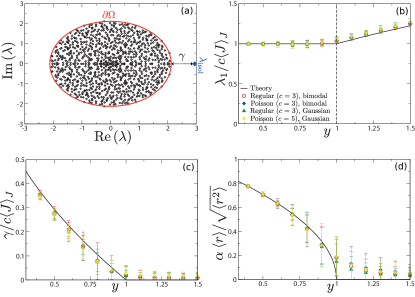
Of particular importance are eigenvalue outliers, which are isolated eigenvalues located outside the continuous (bulk) part of the spectrum (see Fig. 1(a)). Eigenvalue outliers of sparse non-Hermitian random-matrix ensembles, and their associated eigenvectors, are of key interest for studies on the dynamics of complex systems, and for the evaluation of ranking and inference algorithms on graphs. The stationary state of a stochastic process is given by the left eigenvector associated to an outlier of a Markov matrix, the relaxation time is given by the corresponding spectral gap levin2009markov ; monthus , and the large-deviation function of an observable is given by an outlier of a modified Markov matrix donsker1975asymptoticI ; donsker1975asymptoticII ; donsker1976asymptoticIII ; donsker1983asymptoticIV ; de2016rare . Complex dynamical systems, such as, neural networks sompolinsky1988chaos ; rajan2006eigenvalue ; ahmadian2015properties ; aljadeff2015transition or ecosystems may1972will ; allesina2015stability , are often modelled in terms of differential equations coupled through random matrices. The eigenvalue with the largest real part, which is often an outlier, determines the local stability of these systems FootnoteF ; Fyodorov2016 . The PageRank algorithm of Google Search ranks pages of the World Wide Web with the eigenvector associated to the outlier of a generator matrix of a stochastic process langville2011google ; ermann2015google . Spectral algorithms detect communities in sparse graphs based on the eigenvectors of outliers in the spectrum of the non-backtracking matrix krzakala2013spectral ; saade2014spectral ; bordenave2015non . If these outliers exist, then it is possible to detect communities. Conversely, if these outliers do not exist, then it is impossible for any algorithm to detect communities. Quite apart from these applications, the study of outliers of random matrices is also a topic of interest in mathematics tao2013outliers ; bordenave2014outlier .

In this Letter we present a general theory for the outliers of matrices with a local tree structure. We present a set of exact relations for the outliers of sparse non-Hermitian random matrices, and for the left- and right-eigenvector elements associated to the outlier. For oriented random matrices or oriented random graphs, i.e., directed graphs that have no bidirected links, we present explicit expressions for the eigenvalue outliers, the spectral gap, and the first two moments of the distribution of eigenvector elements associated to the outlier. Interestingly, we show that the eigenvalue outliers of oriented random matrices, and the associated eigenvector moments, obey universal expressions.

Outliers of non-Hermitian matrices

We consider an $n\times n$ random matrix $\mbox{\boldmath$A$}_{n}$ with probability density $p(\mbox{\boldmath$A$}_{n})$. The matrix $\mbox{\boldmath$A$}_{n}$ has $n$ complex-valued eigenvalues $\lambda_{1},\cdots,\lambda_{n}$, and its empirical spectral distribution is tao2012topics :

$$\mu_{\mbox{\boldmath$A$}_{n}}=\frac{1}{n}\sum^{n}_{j=1}\delta_{\lambda_{j}}\,,$$ (1)

with $\delta_{\lambda_{j}}$ the Dirac measure, i.e., $\delta_{\lambda_{j}}(S)=0$ when $\lambda_{j}\notin S$ and $\delta_{\lambda_{j}}(S)=1$ when $\lambda_{j}\in S$, with $S$ a Lebesgue-measurable subset of $\mathbb{C}$. We assume that the matrix ensembles considered here are self-averaging, i.e., $\mu_{\mbox{\boldmath$A$}_{n}}\rightarrow\mu$ for $n\rightarrow\infty$, with $\mu$ a deterministic measure. The Lebesgue decomposition theorem hewitt2013real states that $\mu$ consists of an absolute continuous part $\mu_{\rm ac}$, a singular continuous part $\mu_{\rm sing}$, and a pure point part $\mu_{\rm pp}$. The spectral density function $\rho(\lambda)$, also called the density of states, is the probability-density function of $\mu_{\rm ac}$ spec . Its support is the subset $\Omega$ of $\mathbb{C}$ for which $\rho(\lambda)>0$, and $\partial\Omega$ is the boundary of $\Omega$. The measure $\mu_{\rm pp}$ is discrete, i.e., it consists of a collection of Dirac measures, $\mu_{\rm pp}=\sum_{\alpha\in\mathcal{L}}a_{\alpha}\delta_{\lambda_{\alpha}}$, where $\mathcal{L}$ defines a countable set and $a_{\alpha}$ is the weight of the eigenvalue $\lambda_{\alpha}$. The outliers of a random matrix are the values of $\lambda_{\alpha}$ that lie outside the support of the spectral density $\Omega$ ($\lambda_{\alpha}\notin\Omega$). In Fig. 1(a) we show for a random matrix the outlier $\lambda_{\rm isol}$ and the boundary $\partial\Omega$ of the support of the spectral density.

Sparse matrices

We consider a sparse random and non-Hermitian matrix $\mbox{\boldmath$A$}_{n}$. The matrix elements of $\mbox{\boldmath$A$}_{n}$ are $\left[\mbox{\boldmath$A$}_{n}\right]_{jk}=C_{jk}J_{jk}$, with $C_{jk}$ the elements of the adjacency matrix of a random and directed graph bollobas1998random , and $J_{jk}$ complex-valued weights that determine the dynamics of a process on a graph. A connectivity element $C_{jk}$ is equal to either $0$ or $1$; if there is a directed link from vertex $j$ to vertex $k$, then $C_{jk}=1$, whereas if there is no link between the two vertices, then $C_{jk}=0$; we set diagonal elements $C_{ii}$ to one. We consider graph ensembles of finite connectivity, in other words, the outdegrees $K^{\rm out}_{j}=\sum^{n}_{k=1(k\neq j)}C_{jk}$ and the indegrees $K^{\rm in}_{j}=\sum^{n}_{k=1(k\neq j)}C_{kj}$ are finite and independent of $n$. Additionally, we consider that the random graph with adjacency matrix $C_{jk}$ is locally tree-like Bor2010 , which means that a typical neighbourhood of a vertex has no cycles of degree three or higher local . Examples of local tree-like ensembles are the regular directed graph Metz ; Neri2012 , and the directed Erdös-Rényi or Poisson ensemble Rogers2 .

General theory

We present a theory for the outliers $\lambda_{{\rm isol}}$ of locally tree-like random matrices $\mbox{\boldmath$A$}_{n}$, and their corresponding left and right eigenvectors, which we denote by $\langle l_{{\rm isol}}\,|$ and $|\,r_{{\rm isol}}\rangle$, respectively. We first write the right and left eigenvectors of a given outlier $\lambda_{\rm isol}$ in terms of the resolvent $\mathbf{G}_{n}$ of a matrix $\mbox{\boldmath$A$}_{n}$. We define the resolvent $\mathbf{G}_{n}(\lambda)$ of the matrix $\mbox{\boldmath$A$}_{n}$ as

$$\mathbf{G}_{n}(\lambda)\equiv\left(\mbox{\boldmath$A$}_{n}-\lambda\mbox{\boldmath$1$}_{n}\right)^{-1}\,,$$ (2)

with $\lambda\in\mathbb{C}$. The resolvent $\mathbf{G}_{n}$ is singular at the eigenvalues $\lambda=\lambda_{j}$ of $\mbox{\boldmath$A$}_{n}$. Indeed, when we apply the eigen-decomposition theorem to $\mathbf{G}_{n}$, we find

$$\mathbf{G}_{n}=\frac{|\,r_{\rm isol}\rangle\langle l_{\rm isol}\,|}{\lambda_{\rm isol}-\lambda}+\sum^{n}_{j=2}\frac{|\,v^{(r)}_{j}\rangle\langle v^{(l)}_{j}\,|}{\lambda_{j}-\lambda}\,,$$ (3)

with $|\,v^{(r)}_{j}\rangle$ and $\langle v^{(l)}_{j}\,|$, respectively, the right and left eigenvectors associated to $\lambda_{j}$. If we set $\lambda=\lambda_{\rm isol}-i\eta$, with $\eta$ a small real-valued regularizer, then we have

$$\lim_{\eta\rightarrow 0}i\eta\>\mathbf{G}_{n}(\lambda_{\rm isol}-i\eta)=|\,r_{\rm isol}\rangle\langle l_{\rm isol}\,|+\mathcal{O}\left(\eta\right)\,.$$ (4)

Since $\lambda_{\rm isol}$ is an outlier, the relation (4) holds, and is well defined in the infinite-size limit $n\rightarrow\infty$.

We compute the elements of the resolvent $\mathbf{G}_{n}(\lambda-i\eta)$ using the local tree structure of sparse ensembles in the infinite-size limit. The outcome of our procedure is a set of recursive equations for the eigenvector elements $r_{j}=\langle j|\,r_{\rm isol}\rangle$ and $l_{j}=\langle j|\,l_{\rm isol}\rangle$ (see Supplement Supp ):

$$r_{j} = -g_{j}\sum_{k\in\partial_{j}}A_{jk}r^{(j)}_{k}\,,$$ (5)

$$l_{j}^{\ast} = -g_{j}\sum_{k\in\partial_{j}}\left(l^{(j)}_{k}\right)^{\ast}A_{kj}\,,$$ (6)

with the ”neighbourhood” $\partial_{j}$ the set of vertices $k(\neq j)$ for which either $C_{kj}\neq 0$ or $C_{jk}\neq 0$. The variables $g_{j}$ are the diagonal elements of the resolvent $\mathbf{G}_{n}$, i.e., $g_{j}=\left[\mathbf{G}_{n}(\lambda-i\eta)\right]_{jj}$. They solve the equations

$$g_{j} = \frac{1}{-\lambda+i\>\eta+A_{jj}-\sum_{k\in\partial_{i}}A_{jk}\,g^{(j)}_{k}A_{kj}}\,,$$ (7)

$$g^{(\ell)}_{j} = \frac{1}{-\lambda+i\>\eta+A_{jj}-\sum_{k\in\partial_{i}\setminus\left\{\ell\right\}}A_{jk}\,g^{(j)}_{k}A_{kj}}\,,$$ (8)

for $\lambda\notin\Omega$. The random variables $r^{(\ell)}_{j}$ and $l^{(\ell)}_{j}$ in Eqs. (5)-(6) solve

$$r^{(\ell)}_{j} = -g^{(\ell)}_{j}\sum_{k\in\partial_{j}\setminus\left\{\ell\right\}}A_{jk}r^{(j)}_{k}\,,$$ (9)

$$\left(l^{(\ell)}_{j}\right)^{\ast} = -g^{(\ell)}_{j}\sum_{k\in\partial_{j}\setminus\left\{\ell\right\}}\left(l^{(j)}_{k}\right)^{\ast}A_{kj}\,,$$ (10)

with $\ell\in\partial_{j}$. An outlier value $\lambda_{\rm isol}$ is given by a value $\lambda$ for which the Eqs. (5)-(10) admit a non-trivial solution, i.e., a solution for which all eigenvector components $r_{j}$ and $l_{j}^{\ast}$ are neither zero-valued nor infinitely large. The Eqs. (5)-(10) apply to non-Hermitian matrices with a local tree structure, and extend studies on the largest eigenvalue of sparse symmetric matrices Kab2010 ; Kab2012 ; Tak2014 ; Kaw2015 .

Oriented matrices

We illustrate our theory on oriented random-matrix ensembles. Oriented matrices contain only directed links, i.e., $C_{jk}C_{kj}=0$ for all $j\neq k$. For oriented matrices the resolvent Eqs. (7) and (8) simplify and admit the solution

$$g_{j}=g^{(\ell)}_{j}=\left(-\lambda+A_{jj}\right)^{-1}\quad.$$ (11)

The eigenvector components are then given by

$$r_{j} = r^{(\ell)}_{j},\ {\rm for\ all},\ \ell\in\partial^{\rm in}_{j}\,,$$ (12)

$$l_{j} = l^{(\ell)}_{j},\ {\rm for\ all},\ \ell\in\partial^{\rm out}_{j}\,,$$ (13)

where the random variables $r^{(\ell)}_{j}$ and $l^{(\ell)}_{j}$ represent a non-trivial solution to the Eqs. (9)-(10). The ”in-neighbourhood” $\partial^{\rm in}_{j}$ is the set of vertices $k$($\neq j$) with $C_{kj}\neq 0$, and the ”out-neighbourhood” $\partial^{\rm out}_{j}$ is the set of vertices $k$($\neq j$) w ith $C_{jk}\neq 0$.

Figure 1: The outlier $\lambda_{\rm isol}$, spectral gap $\gamma$ and first moment $\langle r\rangle$ of the eigenvector, associated to $\lambda_{\rm isol}$, of oriented adjacency matrices. Direct-diagonalization results of matrices of finite size $n=1000$ (markers) are compared with our theory for infinite-sized matrices, given by Eqs. (14)-(17) (solid lines). Subfigure (a): eigenvalues of one $c$-regular matrix with Gaussian distributed off-diagonal elements, mean degree $c=3$ and $y=0.5$, with $y=\langle J^{2}\rangle_{J}/(c\langle J\rangle_{J}^{2})$ the disorder parameter. The boundary $\partial\Omega$ of the support of the spectral density, the spectral gap $\gamma$ and the outlier $\lambda_{\rm isol}$ are indicated. Subfigures (b)-(d): the eigenvalue $\lambda_{\rm 1}$ with the largest real part, the spectral gap $\gamma$, and the first moment $\langle r\rangle$ of the right eigenvector associated to $\lambda_{1}$, all plotted as a function of $y$. The eigenvalue $\lambda_{1}$ is an outlier for $y<1$, i.e., $\lambda_{1}=\lambda_{\rm isol}$, and $\lambda_{1}\in\partial\Omega$ for $y>1$. Results shown are for four different ensembles of oriented matrices. The ensembles are either $c$-regular or Poissonian with mean connectivity $c$; nonzero off-diagonal elements are i.i.d. with either a bimodal distribution $p_{\rm J}(J)=(1-\Delta)\delta(J+1)+\Delta\delta(J-1)$, or a Gaussian distribution with mean $\langle J\rangle_{J}=1$; diagonal matrix elements are set to zero. Direct diagonalization results in subfigures (b)-(d) are from $1000$ samples. Error bars represent the standard deviation of the sampled population and $\alpha=\sqrt{\langle(K^{\rm out})^{2}\rangle_{K^{\rm out}}-c}/c$.

Figure 2: Probability distribution $p_{\rm R}$ of the right eigenvector elements associated to the outlier of oriented adjacency matrices. The ensembles are the same in Fig.1 with disorder parameter $y=0.4$, and mean connectivity (a) $c=3$, or (b) $c=10$ . We compare direct-diagonalization results (markers) with population-dynamics results (solid lines in (a)) and with the normal distribution (dashed line). Direct-diagonalization results are for $2e+4$ matrix samples of size $n=1000$. In order to show universality of the distribution at high connectivities, we have rescaled the distributions with their mean $\langle r\rangle$ and standard deviation $\sigma_{r}$.

We derive explicit analytical and numerical results by ensemble averaging the Eqs. (12)-(13). An outlier value $\lambda_{\rm isol}$, and its associated eigenvector moments $\langle r^{m}\rangle=N^{-1}\langle\sum^{n}_{j=1}r^{m}_{j}\rangle$ and $\langle l^{m}\rangle=n^{-1}\langle\sum^{n}_{j=1}l^{m}_{j}\rangle$, with $m=1,2$, are given by a non-trivial solution to these ensemble-averaged equations; the symbol $\langle\dots\rangle$ denotes here the ensemble average with respect to the distribution $p(\mbox{\boldmath$A$}_{n})$. Additionally, we can compute the associated ensemble-averaged distribution of eigenvector elements using the population dynamics algorithm abou1973selfconsistent ; cizeau1994theory ; mezard2001bethe ; metz2010localization ; Supp . We illustrate this ensemble-averaging procedure on two paradigmatic examples of sparse matrix ensembles: adjacency matrices and Laplacian matrices of oriented random graphs.

Adjacency matrices

We consider random adjacency matrices $\mbox{\boldmath$A$}_{n}$, which represent an oriented random graph with a given joint distribution $p_{K^{\rm in},K^{\rm out}}$ of in- and outdegrees bollobas1998random ; molloy1995critical ; molloy1998size . The off-diagonal weights $J_{kj}$, with $k\neq j$, are independent and identically distributed (i.i.d.) with distribution $p_{\rm J}$, and the diagonal weights $J_{jj}$ are i.i.d. with distribution $p_{\rm D}$.

The oriented adjacency matrices we consider here have either exactly one outlier (see Fig. 1(a)), or do not have any outlier. If the outlier exists, we call the random-matrix ensemble gapped. Conversely, if the outlier does not exist, we call the ensemble gapless. If the outlier exists, its value $\lambda_{\rm isol}$ solves Supp

$$\Big{\langle}\left(\lambda_{\rm isol}-D\right)^{-1}\Big{\rangle}_{\rm D}=\frac{1}{c\>\langle J\rangle_{\rm J}}\,,$$ (14)

with $\langle\cdot\rangle_{D}$ and $\langle\cdot\rangle_{J}$ denoting, respectively, the average with respect to the distributions $p_{D}$ and $p_{J}$. The quantity $c=\langle K^{\rm in}\rangle_{K^{\rm in}}=\langle K^{\rm out}\rangle_{K^{\rm out}}$ is the mean degree of the graph, where $\langle\cdot\rangle_{K^{\rm in}}$ and $\langle\cdot\rangle_{K^{\rm out}}$ denote averages with respect to the indegree and outdegree distribution, respectively. Equation (14) follows from solving the ensemble averaged version of the Eqs. (5) and (6) for the eigenvector moments. The first two moments of the distribution of right- and left-eigenvector elements read Supp

$$\langle r\rangle^{2}/\langle r^{2}\rangle = \frac{\mathcal{Q}}{\left\langle(K^{\rm out})^{2}\right\rangle_{K_{\rm out}}-c}\,,$$ (15)

$$\langle l\rangle^{2}/\langle l^{2}\rangle = \frac{\mathcal{Q}}{\left\langle(K^{\rm in})^{2}\right\rangle_{K_{\rm in}}-c}\,,$$ (16)

with $\mathcal{Q}=\Big{\langle}\langle J\rangle_{\rm J}^{2}/|\lambda_{\rm isol}-D|^{2}\Big{\rangle}^{-1}_{\rm D}-c\langle J^{2}\rangle_{\rm J}/\langle J\rangle^{2}_{\rm J}$. Additionally, we find the support $\Omega$ of $\rho(\lambda)$ from a stability analysis around the solution (11) to the resolvent Eqs. (7) and (8); the set $\Omega$ contains the values $\lambda\in\mathbb{C}$ with

$$\left\langle\frac{1}{|\lambda-D|^{2}}\right\rangle^{-1}_{D}<c\left\langle J^{2}\right\rangle_{J}\,.$$ (17)

In Fig. 1 we compare the analytical expressions, given by Eqs. (14)-(17), with direct-diagonalization results of matrices of finite size. Results are in good correspondence and converge to the theoretical expressions for large matrix sizes $n\gg 1$ (for which the ensembles become local tree like).

Equations (14)-(17) imply that the outlier of oriented adjacency matrices, and the first moments of its associated eigenvector distribution, are universal. In order to illustrate this universality, we plot in Fig. 1(b)-(d), for different matrix ensembles, the eigenvalue outlier, the spectral gap and the first two moments of the eigenvector distribution, as a function of the disorder parameter $y=\langle J^{2}\rangle_{J}/\left(c\langle J\rangle^{2}_{J}\right)$. The curves for the different ensembles collapse on the universal curve given by our analytical expressions Eqs. (14-17).

A characteristic feature of Fig. 1 is the phase transition from a gapless phase at high disorder, $y>1$, to a gapped phase at low disorder, $y<1$. Note that this phase transition is generic and it also appears in symmetric random matrix ensembles Edwards ; Bassler ; Kab2010 ; Kab2012 ; Tak2014 ; Kaw2015 .

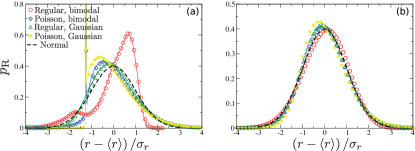
For large mean connectivities, $c\gg 1$, the distributions of right- and left-eigenvector elements become universal, and from Eqs. (5) and (6), it follows that they are Gaussian. In Fig. 2(b) we illustrate the universality of the eigenvector distributions at high connectivities $c$. At low connectivities $c$, the distributions are not universal, but direct-diagonalization results are in good correspondence with numerical solutions of Eqs. (5) and (6) using the population dynamics algorithm (see Fig. 2(a)).

Laplacian matrices

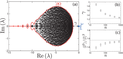
Laplacian matrices are the generator matrices of the dynamics of a random walk on a graph. The defining feature of a Laplacian matrix is the constraint $J_{jj}=-\sum^{n}_{k=1,(k\neq j)}J_{jk}$ on its diagonal elements. Symmetric Laplacian matrices have been studied in Fyodorov2003 ; Kuhn2015 . Here we study the spectra of unnormalized Laplacian matrices of oriented graphs with off-diagonal matrix elements $J_{jk}=1$ and with a given joint degree distribution $p_{K^{\rm in},K^{\rm out}}$ bollobas1998random ; molloy1995critical ; molloy1998size .

The outlier of Laplacian matrices is given by $\lambda_{\rm isol}=0$, and the distribution of right-eigenvector elements reads $p_{\rm R}(r)=\delta(r-1)$. The distribution of left-eigenvector elements $p_{\rm L}(l)$ encodes the statistics of the steady-state probability distribution of a random walk on the associated graph. We take the average of Eqs. (6) and find for the moments of the distribution of left-eigenvector elements (see Supplement Supp ):

$$\frac{\langle l^{2}\rangle}{\langle l\rangle^{2}}=\frac{\left\langle\frac{(K^{\rm in})^{2}-c}{(K^{\rm out})^{2}}\right\rangle_{K^{\rm in},K^{\rm out}}}{\left\langle\frac{c}{K^{\rm out}}\right\rangle^{2}_{K^{\rm out}}-\left\langle\frac{c}{(K^{\rm out})^{2}}\right\rangle_{K^{\rm out}}}\,.$$ (18)

We also derive an expression for the support $\Omega$ of the spectral-density function. We find that $\Omega$ consists of values $\lambda\in\mathbb{C}$ for which either

$$\Bigg{\langle}\frac{K^{\rm out}}{\left|\lambda+K^{\rm out}\right|^{2}}\Bigg{\rangle}_{K^{\rm out}}>1\,,{\rm or}\ \Bigg{\langle}\frac{K^{\rm in}}{\left|\lambda+K^{\rm out}\right|^{2}}\Bigg{\rangle}_{K^{\rm in},K^{\rm out}}>1\,.$$

(19)

In Fig. 3(a) we compare the Eqs. (19) for $\Omega$ with direct-diagonalization results of Laplacian matrices of finite size. We also compare direct-diagonalization results for the spectral gap $\gamma$ and the ratio of the moments $\langle l^{2}\rangle/\langle l\rangle^{2}$ with the exact expressions given by Eqs. (18)-(19). Numerical results converge to the analytical expressions for large matrix sizes $n$.

Figure 3: Results for Laplacian matrices defined on an oriented Erdös-Rényi random graph with off-diagonal matrix elements $J_{kj}=1$ for $k\neq j$. We consider here an ensemble with correlated in- and outdegrees: $p_{K^{\rm in},K^{\rm out}}(k^{\rm in},k^{\rm out})=\delta(k^{\rm in};k)\delta(k^{\rm out};k)p_{\rm deg}(k)$. The degree distribution $p_{\rm deg}(k)$ is Poissonian, i.e., $p_{\rm deg}(k)=\mathcal{N}e^{-\tilde{c}}\tilde{c}^{k}/k!$, if $k\geq k_{0}$, and $p_{\rm deg}(k)=0$ if $k<k_{0}$. Direct diagonalization results (markers) are compared with analytical results (solid lines) for $k_{0}=2$ and $\tilde{c}=4$. Subfigure (a): spectrum of a single matrix with $n=4000$. The red line shows the boundary of the support of the spectral density $\partial\Omega$, given by Eqs. (19). Subfigures  (b)-(c): spectral gap $\gamma$ and moments $\langle l^{2}\rangle/\langle l\rangle^{2}$ are shown to converge to the theoretical values for $n\rightarrow\infty$. Direct diagonalization results are averages over $1e+3$ matrices (markers) and theoretical expressions follow from Eqs. (18)-(19) (dashed lines).

Discussion

We have presented an exact theory for the outliers of random matrices with a local tree structure. Remarkably, for oriented matrices we find general analytical expressions for the outliers, the associated statistics of eigenvectors, and the support of the spectral density. These results show that the spectral properties of outliers of oriented matrices are universal. It will be interesting to explore the implications of these results for the dynamics of complex systems with unidirectional interactions, which often appear in biological systems that operate far from thermal equilibrium, for example, neural networks amit1997dynamics ; brunel2000dynamics or networks of biochemical reactions edwards2000escherichia . Our theory, based on the Eqs. (5)-(10), applies also to non-oriented matrices, and we illustrate this on the elliptic regular ensemble in the supplement Supp . Following Refs. Metz ; Metz2 it is possible to extend our approach to random matrices with many cycles. We expect that studies along these lines will lead to a general theory for the outliers of sparse random matrices.

I.N. thanks José Negrete Jr. for a stimulating discussion.

See pages 1 of SuppMat2.pdf See pages 2 of SuppMat2.pdf See pages 3 of SuppMat2.pdf See pages 4 of SuppMat2.pdf See pages 5 of SuppMat2.pdf See pages 6 of SuppMat2.pdf See pages 7 of SuppMat2.pdf See pages 8 of SuppMat2.pdf See pages 9 of SuppMat2.pdf See pages 10 of SuppMat2.pdf See pages 11 of SuppMat2.pdf See pages 12 of SuppMat2.pdf See pages 13 of SuppMat2.pdf See pages 14 of SuppMat2.pdf See pages 15 of SuppMat2.pdf See pages 16 of SuppMat2.pdf See pages 17 of SuppMat2.pdf See pages 18 of SuppMat2.pdf See pages 19 of SuppMat2.pdf

References

- (1) E. Seneta, Non-negative matrices and Markov chains. Springer Science & Business Media, 2006.
- (2) D. A. Levin, Y. Peres, and E. L. Wilmer, Markov chains and mixing times, ch. 12. American Mathematical Soc., 2009.
- (3) R. Seydel, Practical bifurcation and stability analysis, vol. 5. Springer Science & Business Media, 2009.
- (4) J. Ginibre, “Statistical ensembles of complex, quaternion, and real matrices,” Journal of Mathematical Physics, vol. 6, no. 3, pp. 440–449, 1965.
- (5) V. L. Girko, “The elliptic law,” Teoriya Veroyatnostei i ee Primeneniya, vol. 30, no. 4, pp. 640–651, 1985.
- (6) H. J. Sommers, A. Crisanti, H. Sompolinsky, and Y. Stein, “Spectrum of large random asymmetric matrices,” Phys. Rev. Lett., vol. 60, pp. 1895–1898, 1988.
- (7) J. Feinberg and A. Zee, “Non-gaussian non-hermitian random matrix theory: phase transition and addition formalism,” Nuclear Physics B, vol. 501, no. 3, pp. 643–669, 1997.
- (8) J. Feinberg and A. Zee, “Non-hermitian random matrix theory: method of hermitian reduction,” Nuclear Physics B, vol. 504, no. 3, pp. 579–608, 1997.
- (9) Y. V. Fyodorov, B. A. Khoruzhenko, and H.-J. Sommers, “Almost-hermitian random matrices: eigenvalue density in the complex plane,” Physics Letters A, vol. 226, no. 1, pp. 46–52, 1997.
- (10) R. A. Janik, M. A. Nowak, G. Papp, and I. Zahed, “Non-hermitian random matrix models,” Nuclear Physics B, vol. 501, no. 3, pp. 603–642, 1997.
- (11) G. Akemann, J. Baik, and P. Di Francesco, The Oxford handbook of random matrix theory. Oxford University Press, 2011.
- (12) C. Bordenave, D. Chafaï, “Around the circular law,” Probability surveys, vol. 9, 2012.
- (13) Y. V. Fyodorov, H.-J. Sommers, and B. A. Khoruzhenko, “Universality in the random matrix spectra in the regime of weak non-hermiticity,” Annales de l’I.H.P. Physique théorique, vol. 68, no. 4, pp. 449–489, 1998.
- (14) T. Rogers and I. P. Castillo, “Cavity approach to the spectral density of non-hermitian sparse matrices,” Phys. Rev. E, vol. 79, p. 012101, Jan 2009.
- (15) F. L. Metz, I. Neri, and D. Bollé, “Spectra of sparse regular graphs with loops,” Phys. Rev. E, vol. 84, p. 055101, Nov 2011.
- (16) D. Bollé, F. L. Metz, and I. Neri, Spectral Analysis, Differential Equations and Mathematical Physics: A Festschrift in Honor of Fritz Gesztesy’s 60th Birthday, ch. On the spectra of large sparse graphs with cycles. 2013.
- (17) I. Neri and F. L. Metz, “Spectra of sparse non-hermitian random matrices: An analytical solution,” Phys. Rev. Lett., vol. 109, p. 030602, Jul 2012.
- (18) A. Saade, F. Krzakala, and L. Zdeborová, “Spectral density of the non-backtracking operator on random graphs,” EPL (Europhysics Letters), vol. 107, no. 5, p. 50005, 2014.
- (19) H. Rouault and S. Druckmann, “Spectrum density of large sparse random matrices associated to neural networks,” arXiv preprint arXiv:1509.01893, 2015.
- (20) A. Amir, N. Hatano, and D. R. Nelson, “Non-hermitian localization in biological networks,” Physical Review E, vol. 93, no. 4, p. 042310, 2016.
- (21) C. Monthus and T. Garel, ”An eigenvalue method for computing the largest relaxation time of disordered systems”, J. Stat. Mech. P12017 (2009)
- (22) M. D. Donsker and S. S. Varadhan, “Asymptotic evaluation of certain markov process expectations for large time, i,” Communications on Pure and Applied Mathematics, vol. 28, no. 1, pp. 1–47, 1975.
- (23) M. Donsker and S. Varadhan, “Asymptotic evaluation of certain markov process expectations for large time, ii,” Communications on Pure and Applied Mathematics, vol. 28, no. 2, pp. 279–301, 1975.
- (24) M. Donsker and S. Varadhan, “Asymptotic evaluation of certain markov process expectations for large time—iii,” Communications on pure and applied Mathematics, vol. 29, no. 4, pp. 389–461, 1976.
- (25) M. Donsker and S. Varadhan, “Asymptotic evaluation of certain markov process expectations for large time. iv,” Communications on Pure and Applied Mathematics, vol. 36, no. 2, pp. 183–212, 1983.
- (26) C. De Bacco, A. Guggiola, R. Kühn, and P. Paga, “Rare events statistics of random walks on networks: localisation and other dynamical phase transitions,” Journal of Physics A: Mathematical and Theoretical, vol. 49, no. 18, p. 184003, 2016.
- (27) H. Sompolinsky, A. Crisanti, and H. J. Sommers, “Chaos in random neural networks,” Physical Review Letters, vol. 61, no. 3, p. 259, 1988.
- (28) K. Rajan and L. F. Abbott, “Eigenvalue spectra of random matrices for neural networks,” Physical review letters, vol. 97, no. 18, p. 188104, 2006.
- (29) Y. Ahmadian, F. Fumarola, and K. D. Miller, “Properties of networks with partially structured and partially random connectivity,” Physical Review E, vol. 91, no. 1, p. 012820, 2015.
- (30) J. Aljadeff, M. Stern, and T. Sharpee, “Transition to chaos in random networks with cell-type-specific connectivity,” Physical review letters, vol. 114, no. 8, p. 088101, 2015.
- (31) R. M. May, “Will a large complex system be stable?,” Nature, vol. 238, pp. 413–414, 1972.
- (32) S. Allesina and S. Tang, “The stability–complexity relationship at age 40: a random matrix perspective,” Population Ecology, vol. 57, no. 1, pp. 63–75, 2015.
- (33) The phase of a complex system depends also on the nonlinearity of the differential equations Fyodorov2016 .
- (34) Y. V. Fyodorov and B. A. Khoruzhenko, “Nonlinear analogue of the May-Wigner instability transition”, Proc. Nat. Acad. Sci. USA, vol. 113, no. 25, pp. 6827-6832 (2016).
- (35) A. N. Langville and C. D. Meyer, Google’s PageRank and beyond: The science of search engine rankings. Princeton University Press, 2011.
- (36) L. Ermann, K. M. Frahm, and D. L. Shepelyansky, “Google matrix analysis of directed networks,” Reviews of Modern Physics, vol. 87, no. 4, p. 1261, 2015.
- (37) F. Krzakala, C. Moore, E. Mossel, J. Neeman, A. Sly, L. Zdeborová, and P. Zhang, “Spectral redemption in clustering sparse networks,” Proceedings of the National Academy of Sciences, vol. 110, no. 52, pp. 20935–20940, 2013.
- (38) C. Bordenave, M. Lelarge, and L. Massoulié, “Non-backtracking spectrum of random graphs: community detection and non-regular ramanujan graphs,” in Foundations of Computer Science (FOCS), 2015 IEEE 56th Annual Symposium on, pp. 1347–1357, IEEE, 2015.
- (39) T. Tao, “Outliers in the spectrum of iid matrices with bounded rank perturbations,” Probability Theory and Related Fields, vol. 155, no. 1-2, pp. 231–263, 2013.
- (40) C. Bordenave and M. Capitaine, “Outlier eigenvalues for deformed iid random matrices,” arXiv preprint arXiv:1403.6001, 2014.
- (41) T. Tao, Topics in random matrix theory, vol. 132. American Mathematical Soc., 2012.
- (42) E. Hewitt and K. Stromberg, Real and abstract analysis: a modern treatment of the theory of functions of a real variable. Springer-Verlag, 2013.
- (43) the measure .
- (44) B. Bollobás, “Random graphs,” in Modern Graph Theory, pp. 215–252, Springer, 1998.
- (45) C. Bordenave and M. Lelarge, “Resolvent of large random graphs,” Random Structures and Algorithms, vol. 37, no. 3, pp. 332–352, 2010.
- (46) Loops are typically of size .
- (47) I. Neri and F. L. Metz Supplemental Material: Cavity method for the outlier eigenpair of sparse non-Hermitian random matrices, 2016.
- (48) Y. Weiss and W. T. Freeman, “Correctness of belief propagation in gaussian graphical models of arbitrary topology,” Neural computation, vol. 13, no. 10, pp. 2173–2200, 2001.
- (49) D. Bickson, “Gaussian belief propagation: Theory and application,” arXiv preprint arXiv:0811.2518, 2008.
- (50) J. W. Negele and H. Orland, Quantum many-particle systems, vol. 200. Addison-Wesley New York, 1988.
- (51) I. Neri and D. Bollé, ”The cavity approach to parallel dynamics of Ising spins on a graph”, J. Stat. Mech. P08009 (2009)
- (52) E. Aurell and H. Mahmoudi, “Three lemmas on dynamic cavity method,” Communications in Theoretical Physics, vol. 56, no. 1, p. 157, 2011.
- (53) T. Rogers, I. P. Castillo, R. Kühn, and K. Takeda, “Cavity approach to the spectral density of sparse symmetric random matrices,” Phys. Rev. E, vol. 78, p. 031116, Sep 2008.
- (54) G. Biroli, G. Semerjian, and M. Tarzia, “Anderson model on bethe lattices: density of states, localization properties and isolated eigenvalue,” Progress of Theoretical Physics Supplement, vol. 184, pp. 187–199, 2010.
- (55) Y. Kabashima, H. Takahashi, and O. Watanabe, “Cavity approach to the first eigenvalue problem in a family of symmetric random sparse matrices,” Journal of Physics: Conference Series, vol. 233, no. 1, p. 012001, 2010.
- (56) Y. Kabashima and H. Takahashi, “First eigenvalue/eigenvector in sparse random symmetric matrices: influences of degree fluctuation,” Journal of Physics A: Mathematical and Theoretical, vol. 45, no. 32, p. 325001, 2012.
- (57) H. Takahashi, “Fat-tailed distribution derived from the first eigenvector of a symmetric random sparse matrix,” Journal of Physics A: Mathematical and Theoretical, vol. 47, no. 6, p. 065003, 2014.
- (58) T. Kawamoto and Y. Kabashima, “Limitations in the spectral method for graph partitioning: Detectability threshold and localization of eigenvectors,” Phys. Rev. E, vol. 91, p. 062803, Jun 2015.
- (59) F. L. Metz, I. Neri, and D. Bollé, “Localization transition in symmetric random matrices,” Physical Review E, vol. 82, no. 3, p. 031135, 2010.
- (60) R. Abou-Chacra, D. Thouless, and P. Anderson, “A selfconsistent theory of localization,” Journal of Physics C: Solid State Physics, vol. 6, no. 10, p. 1734, 1973.
- (61) P. Cizeau and J.-P. Bouchaud, “Theory of lévy matrices,” Physical Review E, vol. 50, no. 3, p. 1810, 1994.
- (62) M. Mézard and G. Parisi, “The bethe lattice spin glass revisited,” The European Physical Journal B-Condensed Matter and Complex Systems, vol. 20, no. 2, pp. 217–233, 2001.
- (63) M. Molloy and B. Reed, “A critical point for random graphs with a given degree sequence,” Random structures & algorithms, vol. 6, no. 2-3, pp. 161–180, 1995.
- (64) M. Molloy and B. Reed, “The size of the giant component of a random graph with a given degree sequence,” Combinatorics, probability and computing, vol. 7, no. 03, pp. 295–305, 1998.
- (65) S. F. Edwards and R. C. Jones, “The eigenvalue spectrum of a large symmetric random matrix,” Journal of Physics A: Mathematical and General, vol. 9, no. 10, p. 1595, 1976.
- (66) K. E. Bassler, P. J. Forrester, and N. E. Frankel, “Eigenvalue separation in some random matrix models,” Journal of Mathematical Physics, vol. 50, no. 3, 2009.
- (67) J. Stäring, B. Mehlig, Y. V. Fyodorov and J. M. Luck, “Random symmetric matrices with a constraint: the spectral density of random impedance networks”, Phys. Rev. E, vol. 67, no. 4, p. 047101 (2003).
- (68) Kühn, Reimer. ”Spectra of random stochastic matrices and relaxation in complex systems”, Europhysics Letters, 109, 60003, 2015
- (69) D. J. Amit and N. Brunel, “Dynamics of a recurrent network of spiking neurons before and following learning,” Network: Computation in Neural Systems, vol. 8, no. 4, pp. 373–404, 1997.
- (70) N. Brunel, “Dynamics of sparsely connected networks of excitatory and inhibitory spiking neurons,” Journal of computational neuroscience, vol. 8, no. 3, pp. 183–208, 2000.
- (71) J. Edwards and B. Palsson, “The escherichia coli MG1655 in silico metabolic genotype: its definition, characteristics, and capabilities,” Proceedings of the National Academy of Sciences, vol. 97, no. 10, pp. 5528–5533, 2000.