Can sea quark asymmetry shed light on the orbital angular momentum of the proton?

Abstract

A striking prediction of several extensions of the constituent quark model, including the unquenched quark model, the pion cloud model and the chiral quark model, is a proportionality relationship between the quark sea asymmetry and the orbital angular momentum of the proton. We investigate to which extent a relationship of this kind is corroborated by the experiment, through a systematic comparison between expectations based on models and predictions obtained from a global analysis of hard-scattering data in perturbative Quantum Chromodynamics. We find that the data allows the angular momentum of the proton to be proportional to its sea asymmetry, though with a rather large range of the optimal values of the proportionality coefficient. Typical values do not enable us to discriminate among expectations based on different models. In order to make our comparison conclusive, the extrapolation uncertainties on the proportionality coefficient should be reduced, hopefully by means of accurate measurements in the region of small proton momentum fractions, where the data is currently lacking. Nevertheless, the unquenched quark model predicts that quarks account for a proton spin fraction much larger than that accepted by the conventional wisdom. We explicitly demonstrate that such a discrepancy can be reabsorbed in the unknown extrapolation region, without affecting the description of current data, by imposing the unquenched quark model expectation as a boundary condition in the analysis of the data itself. We delineate how the experimental programs at current and future facilities may shed light on the region of small momentum fractions.

In the last decade, it has been increasingly recognized [1, 2, 3, 4] that the pion cloud in the nucleon could play a leading role in our understanding of both the sea quark asymmetry in the proton and the quark contribution to its total angular momentum. Following angular momentum conservation of the pionic fluctuations of the nucleon, Garvey recently showed [5] that the proton orbital angular momentum, $\Delta L$, should be equal to its associated quark-antiquark sea asymmetry, $\mathcal{A}(p)$, i.e.

$$\Delta L\equiv\mathcal{A}(p)\,\mbox{.}$$ (1)

Though this result was originally obtained for the pion cloud extension of the constituent quark model (CQM), it turned out [6] that it also follows in the unquenched quark model (UQM) [7]. A proportionality between $\Delta L$ and $\mathcal{A}(p)$ is also found in the chiral quark model ($\chi$QM) [8, 9], where, however, the orbital angular momentum is enhanced in comparison to the sea asymmetry, as a consequence of a helicity flip of the quark, so that

$$\Delta L\equiv\frac{3}{2}\mathcal{A}(p)\,\mbox{.}$$ (2)

In the nonperturbative Quantum Chromodynamics (QCD) regime, irrespective of the model adopted to describe the nucleon spin structure, the sum of the proton spin, $\Delta\Sigma$, and its orbital angular momentum, $\Delta L$, must be equal to its total angular momentum, $J$:

$$\Delta\Sigma+2\Delta L\equiv 2J=1\,\mbox{.}$$ (3)

Replacing either Eq. (1) or Eq. (2) in Eq. (3) then allows us to establish a linear relationship between the spin and the sea asymmetry of the proton, which we rewrite in a general way as

$$\Delta\Sigma+\frac{1}{c}\,2\mathcal{A}(p)=1\,\mbox{,}$$ (4)

where $1/c$ is the fraction of sea asymmetry identified with the orbital angular momentum. The values of $c$, $\Delta\Sigma$ and $\mathcal{A}(p)$ are predicted in the CQM, UQM and $\chi$QM so that Eq. (4) is automatically satisfied, and are collected for convenience in Tab. 1.

The aim of this paper is twofold. First, we investigate whether a relation like Eq.(4) is corroborated by the experiment. Such a relation, if proven to be valid, may be used together with Eq. (1) or Eq. (2) to constrain the so far unknown orbital angular momentum of the proton, and eventually it may shed light on the decomposition of its total angular momentum. Second, provided that such a relation is valid, we determine from the experiment the optimum range of values of the coefficient $c$. We will then be able to either discriminate among the model expectations collected in Tab. 1, or discuss the limitations that might prevent such a comparison from being conclusive.

In order to do so, we resort to the perturbative QCD regime, in which $\Delta\Sigma$ and $\mathcal{A}(p)$ can be expressed, respectively, in terms of polarized and unpolarized parton distribution functions (PDFs) of the proton

$$\Delta\Sigma(\mu^{2}) =\int_{0}^{1}dx\sum_{q=u,d,s}\left[\Delta q(x,\mu^{2})+\Delta\bar{q}(x,\mu^{2})\right]\,\mbox{,}$$ (5)

$$\mathcal{A}(p)(\mu^{2}) =\int_{0}^{1}dx\left[\bar{d}(x,\mu^{2})-\bar{u}(x,\mu^{2})\right]\,\mbox{.}$$ (6)

Here $x$ is the momentum fraction of the proton carried by the quark, and $\mu^{2}$ is the energy scale. Both $\Delta\Sigma(\mu^{2})$ and $\mathcal{A}(p)(\mu^{2})$ are measurable quantities, in that polarized and unpolarized PDFs can be defined as matrix elements of gauge-invariant non-local partonic operators. Following factorization [10], PDFs can then be determined in global analyses of measured hard-scattering cross sections (see e.g. Refs. [11, 12]).

Model	Ref.	$\Delta\Sigma$	$\mathcal{A}(p)$	$\Delta L$	$c$
CQM	[5]	$1$	$0$	$0$	$1$
UQM	[7]	$0.676$	$0.162$	$0.162$	$1$
$\chi$QM	[9]	$0.370$	$0.210$	$0.315$	$2/3$

Table 1: The values of the spin fraction, $\Delta\Sigma$, sea asymmetry, $\mathcal{A}(p)$, orbital angular momentum, $\Delta L$, and coefficient $c$, Eq. (8), of the proton according to the CQM, UQM and $\chi$QM.

In the perturbative QCD regime, both $\Delta\Sigma$ and $\mathcal{A}(p)$ depend on the factorization scheme and on the energy scale, and evolve with the latter through the PDFs according to the DGLAP equations [13]. Moreover, the contribution of gluons should be taken into account in the decomposition of the total angular momentum of the proton. A possible realization of such a decomposition is provided by the Jaffe and Manohar sum rule [14]

$$\Delta\Sigma(\mu^{2})+2\Delta G(\mu^{2})+2\left[\Delta L(\mu^{2})+\Delta L_{g}(\mu^{2})\right]\equiv 2J=1\,\mbox{,}$$ (7)

where $\Delta G(\mu^{2})=\int_{0}^{1}dx\,\Delta g(x,\mu^{2})$ and $\Delta L_{g}(\mu^{2})$ are the contributions arising, respectively, from the spin and the orbital angular momentum of the gluon. The former is defined as the first moment of the polarized gluon PDF, $\Delta g$, while the latter can be related [15] to a suitable combination of Generalized Parton Distribution functions (GPDs), which can, in turn, be determined from an analysis of Deeply-Virtual Compton Scattering (DVCS) data. Different decompositions of the total angular momentum of the proton, alternative to Eq. (7), are possible (see Ref. [16] for a review and further details on the measurability of each term in the decomposition).

In general, the perturbative QCD regime is expected to match the nonperturbative QCD regime, provided that a sufficiently small scale $\mu^{2}=\mu_{0}^{2}$ is chosen. An optimal value of $\mu_{0}^{2}$ has been recently derived by matching the high- and low-$\mu^{2}$ behaviors of the strong coupling $\alpha_{s}(\mu^{2})$, as predicted, respectively, by its renormalization group equation in various renormalization schemes and its analytic form in the light-front holographic approach [17]. It turned out that, in the $\overline{\rm MS}$ scheme, $\mu_{0}^{2}\simeq 1$ GeV², which is reasonably not too far above the mass of the proton.

As far as the proton total angular momentum decomposition is concerned, we identify the measurable perturbative quantities $\Delta\Sigma(\mu_{0}^{2})$, $\Delta L(\mu_{0}^{2})$ and $\mathcal{A}(p)(\mu_{0}^{2})$ with their nonperturbative counterparts at $\mu_{0}^{2}=1$ GeV². We note that a determination of $\Delta G(\mu_{0}^{2})$ from a phenomenological analysis of hard scattering data is compatible with zero within uncertainties [18, 19], while very little experimental information is available on $\Delta L(\mu^{2})+\Delta L_{g}(\mu^{2})$. For simplicity, we neglect $\Delta L_{g}$.

Given this identification, we can then scrutinize the validity of Eq. (4). In principle, one could test directly Eqs. (1)-(2). However, in practice this is not achievable because of the lack of experimental information on $\Delta L(\mu_{0}^{2})$. We can then use a determination of $\Delta\Sigma(\mu_{0}^{2})$ and $\mathcal{A}(p)(\mu_{0}^{2})$ from a global QCD analysis of experimental data to determine the coefficient

$$c=\frac{2\mathcal{A}(p)(\mu_{0}^{2})}{1-\Delta\Sigma(\mu_{0}^{2})}\,\mbox{.}$$ (8)

In order to do so, we consider the recent determinations of polarized and unpolarized PDFs performed by the NNPDF collaboration: we use the NNPDFpol1.1 set [19] for the polarized PDFs entering $\Delta\Sigma$ in Eq. (5), and the NNPDF3.0 set [22] for the unpolarized PDFs entering $\mathcal{A}(p)$ in Eq. (6). We use both the polarized and the unpolarized PDF sets are at next-to-leading order (NLO) accuracy in perturbative QCD. In comparison with other PDF sets available in the literature, these are based on a methodology which allows for a faithful estimate of PDF uncertainties, and include most of the available experimental information. Specifically, the bulk of the experimental information on $\Delta\Sigma$ is provided by several data sets on inclusive Deep-Inelastic Scattering (DIS) collected in the last decades in a wealth of experiments at CERN, SLAC, DESY and JLAB (see e.g. Ref. [18] for a review); $\mathcal{A}(p)$ is determined, on top of inclusive DIS (see Sec. 2 in Ref. [22] for a complete list of experiments), from fixed-target Drell-Yan (DY) at Fermilab [23, 24, 25] and from $W$-boson production in proton-(anti)proton collisions at the Tevatron [26] and the Large Hadron Collider (LHC) [27, 28, 29]. The polarized and unpolarized NNPDF sets are the only ones to be determined in a mutually consistent way, though they are derived independently from each other, as it is customary in the field.

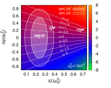
Figure 1: The density plot for the coefficient $c$, Eq (8), obtained by varying the values of $\Delta\Sigma$ and $\mathcal{A}(p)$ at $\mu_{0}^{2}=1$ GeV² within their uncertainties. The values of $\Delta\Sigma$ and $\mathcal{A}(p)$ are obtained according to Eqs. (5)-(6) from the NNPDFpol1.1 [19] and NNPDF3.0 [22] PDF sets respectively. The best fit value of $c$, corresponding to the central values of $\Delta\Sigma$ and $\mathcal{A}(p)$, is also shown, and is labelled NNPDF. The shaded ellipses correspond to their $68\%$ and $90\%$ confidence regions, assuming that $\Delta\Sigma$ and $\mathcal{A}(p)$ are fully uncorrelated. Predictions from the $\chi$QM and UQM are also displayed according to Tab. 1.

In Fig. 1, we show the density plot for the coefficient $c$, Eq (8), obtained by varying the values of $\Delta\Sigma$ and $\mathcal{A}(p)$, Eqs. (5)-(6), within their uncertainties at $\mu_{0}^{2}=1$ GeV². The values of $\Delta\Sigma$ and $\mathcal{A}(p)$ are

$$\Delta\Sigma\,(\mu_{0}^{2}=1\ \rm{GeV}^{2}) = +0.230\pm 0.088\,,$$ (9)

$$\mathcal{A}(p)\,(\mu_{0}^{2}=1\ \rm{GeV}^{2}) = -0.005\pm 0.565\,\mbox{.}$$ (10)

It then follows from Eq. (8) that

$$c=-0.013\pm 1.468\,\mbox{,}$$ (11)

where the uncertainty on $c$ is given at $68\%$ confidence level (CL), and has been obtained by propagating the uncertainty on $\Delta\Sigma$ and $\mathcal{A}(p)$ with the assumption that the two quantities are fully uncorrelated. The point corresponding to these values is denoted as NNPDF in Fig. 1. The corresponding $68\%$ and $90\%$ confidence regions are represented by shaded ellipses. Predictions from the $\chi$QM and UQM are also displayed according to the values in Tab. 1.

Inspection of Fig. 1, together with a comparison among Eqs. (9)-(10)-(11) and the values in Tab. 1, reveals that the current determination of $\Delta\Sigma$ and $\mathcal{A}(p)$ from experimental data could discriminate among different models. Specifically, both the CQM and UQM turn out to be disfavored, in that they predict a value of $\Delta\Sigma$ which is rather larger than that derived from the experiment. Conversely, the predicted value of $\mathcal{A}(p)$ agrees with its experimental counterpart. In the case of the $\chi$QM, by contrast, predictions for both $\Delta\Sigma$ and $\mathcal{A}(p)$ fall very well within the NNPDF $90\%$ confidence region.

In spite of the discrepancy between the experiment and the CQM/UQM predictions for $\Delta\Sigma$ and $\mathcal{A}(p)$, it is worth noting that a relation like Eq. (4) is not ruled out by the experiment. Interestingly, the solution $c=1$, which corresponds to Eq. 1, and is a remarkable prediction of these models, is well compatible with the experiment. A different balance between $\Delta\Sigma$ and $\mathcal{A}(p)$ in the UQM would, however, be needed in order to reconcile their predictions with the experiment. The solution $c=2/3$, predicted by the $\chi$QM, is also allowed by the experiment.

It is worth noting that, following the definitions provided by Eqs. (5)-(6), the results given in Eqs. (9)-(10)-(11) and in Fig. 1 are obtained by integrating the relevant combinations of polarized or unpolarized PDFs over all the range of $x$. However, the available piece of experimental information used to constrain those PDFs only covers a limited range in $x$, roughly $10^{-3}\lesssim x\lesssim 0.5$. In order to assess the impact of the extrapolation of the PDFs into the unknown small-$x$ region on our determination of $\Delta\Sigma$, $\mathcal{A}(p)$ and $c$, Eqs. (9)-(10)-(11), we define the truncated moments of the polarized singlet and unpolarized sea asymmetry PDF combinations

$$\Delta\Sigma^{[x_{\rm min},1]}(\mu^{2}) =\int_{x_{\rm min}}^{1}dx\sum_{q=u,d,s}\left[\Delta q(x,\mu^{2})+\Delta\bar{q}(x,\mu^{2})\right]\,\mbox{,}$$ (12)

$$\mathcal{A}(p)^{[x_{\rm min},1]}(\mu^{2}) =\int_{x_{\rm min}}^{1}dx\left[\bar{d}(x,\mu^{2})-\bar{u}(x,\mu^{2})\right]\,\mbox{.}$$ (13)

These are the counterparts of Eqs. (5)-(6), expressed as a function of the low limit of integration $x_{\rm min}$.

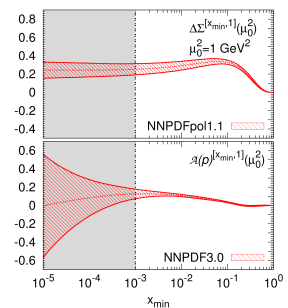
Figure 2: The truncated moments of the polarized singlet and unpolarized sea asymmetry PDF combinations, $\Delta\Sigma^{[x_{\rm min},1]}(\mu_{0}^{2})$ (top) and $\mathcal{A}(p)^{[x_{\rm min},1]}(\mu_{0}^{2})$ (bottom) as a function of $x_{\rm min}$. These are computed by using, respectively, the NNDPFpol1.1 and NNPDF3.0 PDF sets at $\mu_{0}^{2}=1$ GeV². The small-$x$ extrapolation region, in which no relevant experimental information is available, is shaded.

In Fig. 2, we display $\Delta\Sigma^{[x_{\rm min},1]}(\mu_{0}^{2})$ and $\mathcal{A}(p)^{[x_{\rm min},1]}(\mu_{0}^{2})$ as a function of $x_{\rm min}$. They are computed respectively using the NNDPFpol1.1 and NNPDF3.0 PDF sets at $\mu_{0}^{2}=1$ GeV². It then becomes apparent what the impact of the PDF extrapolation into the unknown small-$x$ region is on the determination of $\Delta\Sigma$ and $\mathcal{A}(p)$. In the case of $\Delta\Sigma$, both the central value and the uncertainty of the truncated moment, Eq. (12), converge to the central value and the uncertainty of its corresponding full moment, Eq. (5), below $x_{\rm min}\sim 10^{-3}$. This is a consequence of the fact that the polarized singlet PDF combination is suppressed at small $x$. The contribution to $\Delta\Sigma$ coming from the small-$x$ extrapolation region is thus negligible, as it is also apparent when comparing

$$\Delta\Sigma^{[10^{-3},1]}(\mu_{0}^{2})=0.238\pm 0.080\,\mbox{,}$$ (14)

obtained from the NNPDFpol1.1 PDF set at $\mu_{0}^{2}=1$ GeV², with the full $\Delta\Sigma$, Eq. (9). In the case of $\mathcal{A}(p)$, by contrast, no convergence is reached, at least above $x\sim 10^{-5}$. This is a consequence of the fact that antiquark PDFs grow at small $x$, and that the lack of experimental data does not allow us to tame this growth. The contribution to $\mathcal{A}(p)$ coming from the small-$x$ extrapolation has a significant impact on both the central value and the uncertainty of $\mathcal{A}(p)$, as it is apparent when comparing

$$\mathcal{A}(p)^{[10^{-3},1]}(\mu_{0}^{2})=0.126\pm 0.052\,\mbox{,}$$ (15)

obtained from the NNPDF3.0 PDF set at $\mu_{0}^{2}=1$ GeV², with the full $\mathcal{A}(p)$, Eq. (10). The value in Eq.(15) is consistent with the experimental determination derived, in a similarly limited $x$ region, in dedicated analyses performed either by NMC [30, 31, 32] from inclusive DIS data, or by HERMES [33] from semi-inclusive DIS (SIDIS) data, or by E866 [25, 34], from fixed-target DY data.

Likewise, the value of the coefficient $c$ in Eq. (8) is affected by the extrapolation of the PDFs into the small-$x$ region. Specifically, if we use for $\Delta\Sigma$ and $\mathcal{A}(p)$ their truncated values, Eqs. (14)-(15), rather than their full values, Eqs. (9)-(10), we obtain

$$c^{[10^{-3},1]}\equiv\frac{2\mathcal{A}(p)^{[10^{-3},1]}(\mu_{0}^{2})}{1-\Delta\Sigma^{[10^{-3},1]}(\mu_{0}^{2})}=0.331\pm 0.141\,\mbox{.}$$ (16)

This value is not compatible with any of the model predictions presented in Tab. 1, which then all fall outside the reduced confidence region delimited by the truncated moments Eqs. (9)-(10). Specifically, all models are unable to simultaneously describe $\Delta\Sigma^{[10^{-3},1]}$ and $\mathcal{A}(p)^{[10^{-3},1]}$: the NNPDF value of the former is well reproduced by the $\chi$QM but is greatly overshot by the UQM; the value of the latter is well reproduced by the UQM but slightly overestimated by the $\chi$QM.

We now turn to a further investigation of the largest discrepancy we have found so far, namely that between the UQM and the PDF determination of $\Delta\Sigma$. In order to do so, we revisit the polarized NNPDF analysis used to derive Eqs. (9)-(14). Specifically, we perform three new fits of polarized PDFs, based on a wealth of inclusive DIS data from CERN, SLAC, DESY and JLAB. The full breakdown of the experiments included in our analysis, together with the corresponding number of data points, is outlined in Tab. 2. The data set considered is not exactly the same as in the original NNPDFpol1.1 analysis: here we add the CMP-p(’15) [35] and the JLAB [36, 37, 38] data, which was not available when the NNPDFpol1.1 PDF set was determined. Also, we do not consider data from open-charm leptoproduction in semi-inclusive DIS or from jet and $W$-boson production in polarized $pp$ collisions, which were, instead, included in NNPDFpol1.1. This piece of data constrains the polarized gluon and antiquark PDFs. However they will not affect our conclusions below.

Experiment	Ref.	$N_{\rm dat}$	$\chi^{2}_{1}/N_{\rm dat}$	$\chi^{2}_{2}/N_{\rm dat}$	$\chi^{2}_{3}/N_{\rm dat}$
EMC	[39]	10	0.42	0.42	0.45
SMC	[40]	24	0.93	1.08	1.19
SMClowx	[41]	16	0.95	0.97	0.98
E142	[42]	8	0.56	0.60	0.67
E143	[43]	52	0.63	0.65	0.65
E154	[44]	11	0.31	0.50	0.54
E155	[45]	42	0.94	0.96	0.91
CMP-d	[46]	15	0.55	0.90	1.29
CMP-p	[47]	15	0.94	0.88	0.85
CMP-p(’15)	[35]	51	0.66	0.64	0.61
HERMES-n	[48]	9	0.24	0.27	0.25
HERMES	[49]	58	0.61	0.67	0.69
JLAB-E06-014	[36]	2	1.69	0.86	0.80
JLAB-EG1-DVCS	[37]	18	0.25	0.23	0.28
JLAB-E93-009	[38]	148	0.93	0.95	0.97
TOTAL		479	0.74	0.76	0.79

Table 2: The values of the $\chi^{2}$ per data point, $\chi^{2}_{i}/N_{\rm dat}$, per each experiment included in the three fits described in the text, $i=1,2,3$.

All the three fits are based on the same set of data outlined in Tab. 2, and are performed according to the methodology discussed in Refs. [18, 50]. The three fits differ from one another only with regard to the theoretical assumptions made on the values of the first moments of specific PDF combinations.

FIT1

As in the NNPDFpol1.1 analysis, we require that the first moments of the scale-invariant $C$-even nonsinglet combinations are equal to the measured values of the baryon octet decay constants [51], with an inflated uncertainty on $\Delta T_{8}$ which allows for a potential SU(3) symmetry breaking

$$\Delta T_{3}=1.2701\pm 0.0025\,,\ \ \ \ \ \Delta T_{8}=0.585\pm 0.176\,.$$ (17)

FIT 2

We require that the first moments of total $u$, $d$ and $s$ PDF combinations at $\mu_{0}^{2}=1$ GeV² be equal to the values determined in the UQM [7] with an inflated $20\%$ theoretical uncertainty

$$\Delta U^{+} = +1.098\pm 0.220\,,\ \ \ \ \ \Delta D^{+}=-0.417\pm 0.084\,,\$$

$$\Delta S^{+} = -0.005\pm 0.001\,.$$ (18)

FIT 3

As FIT2, but with a UQM without strangeness [6]

$$\Delta U^{+} = +1.132\pm 0.226\,,\ \ \ \ \ \Delta D^{+}=-0.368\pm 0.074\,,\$$

$$\Delta S^{+} = 0\,.$$ (19)

In Eqs. (17)-(18)-(19) we have defined: $\Delta Q^{+}=\int_{0}^{1}dx\,\Delta q^{+}$, $Q=U,D,S$, with $\Delta q^{+}=\Delta q+\Delta\bar{q}$, $q=u,d,s$; $\Delta T_{3}=\int_{0}^{1}dx\,\left(\Delta u^{+}-\Delta d^{+}\right)$; and $\Delta T_{8}=\int_{0}^{1}dx\,\left(\Delta u^{+}+\Delta d^{+}-2\Delta s^{+}\right)$. As in the original NNPDFpol1.1 analysis, in all these fits we impose that PDFs be integrable, as they should be in order to ensure that the nucleon matrix element of the axial current remains finite for each flavor. We also observe that the values of $\Delta U^{+}$, $\Delta D^{+}$ and $\Delta S^{+}$ imposed either in FIT2 or in FIT1 lead to values of $\Delta T_{3}$ and $\Delta T_{8}$ compatible with those imposed in FIT1.

Because we expect $\Delta\Sigma$ in FIT1 to be statistically equivalent to $\Delta\Sigma$ in the original NNPDF analysis, except for small fluctuations due to the slightly different data set used, we consider it as a baseline, with which we compare FIT2 and FIT3. In Tab. 2, we collect the values of the $\chi^{2}$ per data point, $\chi^{2}_{i}/N_{\rm dat}$, for each experiment included in the three fits, $i=1,2,3$. The values of the relevant corresponding first moments at $\mu_{0}^{2}=1$ GeV² are given in Tab. 3.

MOMs.	FIT1	FIT2	FIT3
$\Delta\Sigma$	$+0.230\pm 0.094$	$+0.636\pm 0.143$	$+0.730\pm 0.163$
$\Delta G$	$-0.587\pm 5.467$	$+5.675\pm 7.057$	$+7.577\pm 8.924$
$\Delta T_{3}$	$+1.270\pm 0.003$	$+1.455\pm 0.277$	$+1.482\pm 0.269$
$\Delta T_{8}$	$+0.579\pm 0.151$	$+0.674\pm 0.144$	$+0.731\pm 0.152$
$\Delta U^{+}$	$+0.807\pm 0.044$	$+1.046\pm 0.152$	$+1.104\pm 0.151$
$\Delta D^{+}$	$-0.456\pm 0.044$	$-0.385\pm 0.138$	$-0.364\pm 0.148$
$\Delta S^{+}$	$-0.114\pm 0.072$	$-0.015\pm 0.078$	$-0.001\pm 0.005$

Table 3: The values of the first moments computed from the three fits discussed in the text at $\mu_{0}^{2}=1$ GeV².

First of all, we observe that the values of the first moments obtained from each fit reproduce, within uncertainties, the corresponding values imposed in the fits themselves. In the case of FIT1, the value of $\Delta\Sigma$ is perfectly consistent with that obtained in the NNPDFpol1.1 analysis, see Eq. (9), though a slightly larger uncertainty is found because of the different data set. Interestingly, in the case of FIT2 and FIT3 the values of $\Delta T_{3}$ and $\Delta T_{8}$, which follow from the UQM predictions, are compatible with the corresponding experimental values in Eq. (17).

Second, we are able to achieve a comparable fit quality in all the three cases: indeed, we do not observe any significant deterioration of the $\chi^{2}$ per data point when moving from the baseline fit to FIT2 and FIT3. We then conclude that it is still possible to reconcile the UQM prediction for $\Delta\Sigma$ with the experimental information available so far. The model and the data are accommodated in the various fits by means of a different extrapolation of the PDFs in the unknown small-$x$ region, with the preferred extrapolation fixed by the values of the first moments imposed in the fit. The differences in the values of $\Delta\Sigma$ among FIT1, FIT2 and FIT3 are then accounted for by a different contribution to the integral in Eq. (5) in the unmeasured region $x\in[0,10^{-3}]$, see Fig. 3. Interestingly, we observe that an extrapolation of $\Delta\Sigma$ similar to that which we obtain in FIT2 and FIT3 has been recently suggested in Ref. [52] by solving suitable small-$x$ evolution equations derived in the framework of polarization-dependent Wilson line-like operators [53, 54].

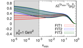
Figure 3: The truncated moment of the polarized singlet PDF combination, $\Delta\Sigma^{[x_{\rm min},1]}(\mu_{0}^{2})$ as a function of $x_{\rm min}$, computed at $\mu_{0}^{2}=1$ GeV² from the various fits described in the text. The small-$x$ extrapolation region, in which no relevant experimental information is available, is shaded.

The different extrapolation of $\Delta\Sigma$ in the unknown small-$x$ region has at least two consequences. On the one hand, because the singlet PDF combination and the gluon PDF are coupled in the evolution equations, we observe a rise in the expected value of $\Delta G$ in FIT2 and FIT3 in comparison with FIT1, though this remains compatible with zero within uncertainties. This large fluctuation is not surprising, because scaling violations, through which the gluon PDF is determined on the basis of the data set considered, only provide a mild constraint. We leave it to a future work to carry out a quantitative study on how much this picture changes if the small-$x$ evolution equations derived in Refs. [53, 54] are included in a global determination of polarized PDFs. On the other hand, the confidence region analogous to that in Fig. 1 nicely includes the UQM expectations for FIT2 and FIT3. The full and truncated values of $c$ and $c^{[10^{-3},1]}$, Eqs. (8)-(16), are, for FIT2 and FIT3 respectively,

$$c_{2}=-0.027\pm 3.104\,, \ \ \ \ \ c_{2}^{[10^{-3},1]}=0.423\pm 0.199\,,$$ (20)

$$c_{3}=-0.011\pm 4.185\,, \ \ \ \ \ c_{3}^{[10^{-3},1]}=0.463\pm 0.248\,,$$ (21)

while for FIT1 we recover similar values to those in Eqs. (11)-(16). Note that the range of allowed values of $c$ is now significantly larger than in Eq. (11), as a consequence of the inflated theoretical uncertainty of the UQM first moments imposed in the fits. All these values are a fortiori compatible with the model expectations in Tab. 1. Slighter fluctuations are observed for the allowed values of $c^{[10^{-3},1]}$ in comparison with Eq. (16), with only $c_{3}^{[10^{-3},1]}$ compatible with the $\chi$QM expectation and neither $c_{2}^{[10^{-3},1]}$ nor $c_{3}^{[10^{-3},1]}$ compatible with the UQM expectations.

Can sea quark asymmetry shed light on the orbital angular momentum of the proton? Our study indicates that the accuracy and the precision with which $\Delta\Sigma$ and $\mathcal{A}(p)$ can be determined from the data is insufficient either to discriminate among models or to put a significant constraint on the coefficient $c$. The main limiting factor in such a program is the lack of experimental information at small values of $x$, which allows for a wealth of largely uncertain extrapolations. We have explicitly demonstrated that these can include values of $\Delta\Sigma$ up to $0.6-0.7$, as predicted e.g. by the UQM or small-$x$ evolution, which are rather larger than $0.2-0.3$, as accepted by the conventional wisdom.

A significant improvement in the experimental coverage of the small-$x$ region is expected in the future for both $\Delta\Sigma$ and $\mathcal{A}(p)$. As far as $\Delta\Sigma$ is concerned, in the long term, inclusive DIS measurements at a future Electron-Ion Collider (EIC) [55] will reach values of $x$ down to $x\sim 10^{-5}$, thus placing a direct constraint on the range of possible extrapolations. The EIC will also be able to pin down the uncertainty on $\Delta\Sigma$ by a factor of two [56, 57, 58]. As far as $\mathcal{A}(p)$ is concerned, in the short term, a reduction of its uncertainty at low values of $x$ is likely to be achieved thanks to $W$-boson production data in $pp$ collisions at the LHC, as well as in fixed-target DY at the dedicated high-precision Fermilab-SeaQuest experiment [59] and at J-PARC [60]; in the long term, brand new experimental facilities, like a Large Hadron electron Collider (LHeC) [61], will explore with unprecedented precision the region of small momentum fractions $x$. An analysis of these data sets will then allow for a further scrutiny of Eq. (4), and eventually place a stringent bound on the acceptable values of $c$. Hopefully, polarized and unpolarized data might be analyzed simultaneously, in order to enable an estimation of the correlations between $\Delta\Sigma$ and $\mathcal{A}(p)$.

The work of E.R.N. is supported by a STFC Rutherford Grant ST/M003787/1.

References

References

- [1] S. Kumano, Flavor asymmetry of anti-quark distributions in the nucleon, Phys. Rept. 303 (1998) 183–257. arXiv:hep-ph/9702367, doi:10.1016/S0370-1573(98)00016-7.
- [2] J. Speth, A. W. Thomas, Mesonic contributions to the spin and flavor structure of the nucleon, Adv. Nucl. Phys. 24 (1997) 83–149. doi:10.1007/0-306-47073-X_2.
- [3] G. T. Garvey, J.-C. Peng, Flavor asymmetry of light quarks in the nucleon sea, Prog. Part. Nucl. Phys. 47 (2001) 203–243. arXiv:nucl-ex/0109010, doi:10.1016/S0146-6410(01)00155-7.
- [4] W.-C. Chang, J.-C. Peng, Flavor Structure of the Nucleon Sea, Prog. Part. Nucl. Phys. 79 (2014) 95–135. arXiv:1406.1260, doi:10.1016/j.ppnp.2014.08.002.
- [5] G. T. Garvey, Orbital Angular Momentum in the Nucleon, Phys. Rev. C81 (2010) 055212. arXiv:1001.4547, doi:10.1103/PhysRevC.81.055212.
- [6] R. Bijker, E. Santopinto, Valence and sea quarks in the nucleon, J. Phys. Conf. Ser. 578 (1) (2015) 012015. arXiv:1412.5559, doi:10.1088/1742-6596/578/1/012015.
- [7] R. Bijker, E. Santopinto, E. Santopinto, Unquenched quark model for baryons: Magnetic moments, spins and orbital angular momenta, Phys. Rev. C80 (2009) 065210. arXiv:0912.4494, doi:10.1103/PhysRevC.80.065210.
- [8] E. J. Eichten, I. Hinchliffe, C. Quigg, Flavor asymmetry in the light quark sea of the nucleon, Phys. Rev. D45 (1992) 2269–2275. doi:10.1103/PhysRevD.45.2269.
- [9] T. P. Cheng, L.-F. Li, Flavor and spin contents of the nucleon in the quark model with chiral symmetry, Phys. Rev. Lett. 74 (1995) 2872–2875. arXiv:hep-ph/9410345, doi:10.1103/PhysRevLett.74.2872.
- [10] J. C. Collins, D. E. Soper, G. F. Sterman, Factorization of Hard Processes in QCD, Adv. Ser. Direct. High Energy Phys. 5 (1989) 1–91. arXiv:hep-ph/0409313, doi:10.1142/9789814503266_0001.
- [11] S. Forte, G. Watt, Progress in the Determination of the Partonic Structure of the Proton, Ann. Rev. Nucl. Part. Sci. 63 (2013) 291–328. arXiv:1301.6754, doi:10.1146/annurev-nucl-102212-170607.
- [12] E. R. Nocera, Achievements and open issues in the determination of polarized parton distribution functions, Int. J. Mod. Phys. Conf. Ser. 40 (2016) 1660016. arXiv:1503.03518, doi:10.1142/S2010194516600168.
- [13] G. Altarelli, G. Parisi, Asymptotic Freedom in Parton Language, Nucl. Phys. B126 (1977) 298–318. doi:10.1016/0550-3213(77)90384-4.
- [14] R. L. Jaffe, A. Manohar, The G(1) Problem: Fact and Fantasy on the Spin of the Proton, Nucl. Phys. B337 (1990) 509–546. doi:10.1016/0550-3213(90)90506-9.
- [15] S. Boffi, B. Pasquini, Generalized parton distributions and the structure of the nucleon, Riv. Nuovo Cim. 30 (2007) 387. arXiv:0711.2625, doi:10.1393/ncr/i2007-10025-7.
- [16] E. Leader, C. Lorcé, The angular momentum controversy: What’s it all about and does it matter?, Phys. Rept. 541 (2014) 163–248. arXiv:1309.4235, doi:10.1016/j.physrep.2014.02.010.
- [17] A. Deur, S. J. Brodsky, G. F. de Teramond, On the Interface between Perturbative and Nonperturbative QCD, Phys. Lett. B757 (2016) 275–281. arXiv:1601.06568, doi:10.1016/j.physletb.2016.03.077.
- [18] R. D. Ball, S. Forte, A. Guffanti, E. R. Nocera, G. Ridolfi, J. Rojo, Unbiased determination of polarized parton distributions and their uncertainties, Nucl. Phys. B874 (2013) 36–84. arXiv:1303.7236, doi:10.1016/j.nuclphysb.2013.05.007.
- [19] E. R. Nocera, R. D. Ball, S. Forte, G. Ridolfi, J. Rojo, A first unbiased global determination of polarized PDFs and their uncertainties, Nucl. Phys. B887 (2014) 276–308. arXiv:1406.5539, doi:10.1016/j.nuclphysb.2014.08.008.
- [20] D. de Florian, R. Sassot, M. Stratmann, W. Vogelsang, Evidence for polarization of gluons in the proton, Phys. Rev. Lett. 113 (1) (2014) 012001. arXiv:1404.4293, doi:10.1103/PhysRevLett.113.012001.
- [21] E.-C. Aschenauer, et al., The RHIC SPIN Program: Achievements and Future OpportunitiesarXiv:1501.01220.
- [22] R. D. Ball, et al., Parton distributions for the LHC Run II, JHEP 04 (2015) 040. arXiv:1410.8849, doi:10.1007/JHEP04(2015)040.
- [23] J. C. Webb, et al., Absolute Drell-Yan dimuon cross-sections in 800 GeV / c pp and pd collisionsarXiv:hep-ex/0302019.
-
[24]
J. C. Webb,
Measurement
of continuum dimuon production in 800-GeV/C proton nucleon collisions,
Ph.D. thesis, New Mexico State U. (2003).
arXiv:hep-ex/0301031.
URL http://lss.fnal.gov/cgi-bin/find_paper.pl?thesis-2002-56 - [25] R. S. Towell, et al., Improved measurement of the anti-d / anti-u asymmetry in the nucleon sea, Phys. Rev. D64 (2001) 052002. arXiv:hep-ex/0103030, doi:10.1103/PhysRevD.64.052002.
- [26] T. Aaltonen, et al., Direct Measurement of the Production Charge Asymmetry in Collisions at TeV, Phys. Rev. Lett. 102 (2009) 181801. arXiv:0901.2169, doi:10.1103/PhysRevLett.102.181801.
- [27] S. Chatrchyan, et al., Measurement of the electron charge asymmetry in inclusive production in collisions at TeV, Phys. Rev. Lett. 109 (2012) 111806. arXiv:1206.2598, doi:10.1103/PhysRevLett.109.111806.
- [28] R. Aaij, et al., Inclusive and production in the forward region at TeV, JHEP 06 (2012) 058. arXiv:1204.1620, doi:10.1007/JHEP06(2012)058.
- [29] G. Aad, et al., Measurement of inclusive jet and dijet production in collisions at TeV using the ATLAS detector, Phys. Rev. D86 (2012) 014022. arXiv:1112.6297, doi:10.1103/PhysRevD.86.014022.
- [30] P. Amaudruz, et al., The Gottfried sum from the ratio F2(n) / F2(p), Phys. Rev. Lett. 66 (1991) 2712–2715. doi:10.1103/PhysRevLett.66.2712.
- [31] M. Arneodo, et al., A Reevaluation of the Gottfried sum, Phys. Rev. D50 (1994) R1–R3. doi:10.1103/PhysRevD.50.R1.
- [32] M. Arneodo, et al., Accurate measurement of F2(d) / F2(p) and R**d - R**p, Nucl. Phys. B487 (1997) 3–26. arXiv:hep-ex/9611022, doi:10.1016/S0550-3213(96)00673-6.
- [33] K. Ackerstaff, et al., The Flavor asymmetry of the light quark sea from semiinclusive deep inelastic scattering, Phys. Rev. Lett. 81 (1998) 5519–5523. arXiv:hep-ex/9807013, doi:10.1103/PhysRevLett.81.5519.
- [34] E. A. Hawker, et al., Measurement of the light anti-quark flavor asymmetry in the nucleon sea, Phys. Rev. Lett. 80 (1998) 3715–3718. arXiv:hep-ex/9803011, doi:10.1103/PhysRevLett.80.3715.
- [35] C. Adolph, et al., The spin structure function of the proton and a test of the Bjorken sum rule, Phys. Lett. B753 (2016) 18–28. arXiv:1503.08935, doi:10.1016/j.physletb.2015.11.064.
- [36] D. S. Parno, et al., Precision Measurements of in the Deep Inelastic Regime, Phys. Lett. B744 (2015) 309–314. arXiv:1406.1207, doi:10.1016/j.physletb.2015.03.067.
- [37] Y. Prok, et al., Precision measurements of of the proton and the deuteron with 6 GeV electrons, Phys. Rev. C90 (2) (2014) 025212. arXiv:1404.6231, doi:10.1103/PhysRevC.90.025212.
- [38] N. Guler, et al., Precise determination of the deuteron spin structure at low to moderate with CLAS and extraction of the neutron contribution, Phys. Rev. C92 (5) (2015) 055201. arXiv:1505.07877, doi:10.1103/PhysRevC.92.055201.
- [39] J. Ashman, et al., An Investigation of the Spin Structure of the Proton in Deep Inelastic Scattering of Polarized Muons on Polarized Protons, Nucl. Phys. B328 (1989) 1. doi:10.1016/0550-3213(89)90089-8.
- [40] B. Adeva, et al., Spin asymmetries A(1) and structure functions g1 of the proton and the deuteron from polarized high-energy muon scattering, Phys. Rev. D58 (1998) 112001. doi:10.1103/PhysRevD.58.112001.
- [41] B. Adeva, et al., Spin asymmetries A(1) of the proton and the deuteron in the low x and low Q**2 region from polarized high-energy muon scattering, Phys. Rev. D60 (1999) 072004, [Erratum: Phys. Rev.D62,079902(2000)]. doi:10.1103/PhysRevD.60.072004,10.1103/PhysRevD.62.079902.
- [42] P. L. Anthony, et al., Deep inelastic scattering of polarized electrons by polarized He-3 and the study of the neutron spin structure, Phys. Rev. D54 (1996) 6620–6650. arXiv:hep-ex/9610007, doi:10.1103/PhysRevD.54.6620.
- [43] K. Abe, et al., Measurements of the proton and deuteron spin structure functions g(1) and g(2), Phys. Rev. D58 (1998) 112003. arXiv:hep-ph/9802357, doi:10.1103/PhysRevD.58.112003.
- [44] K. Abe, et al., Precision determination of the neutron spin structure function g1(n), Phys. Rev. Lett. 79 (1997) 26–30. arXiv:hep-ex/9705012, doi:10.1103/PhysRevLett.79.26.
- [45] P. L. Anthony, et al., Measurements of the Q**2 dependence of the proton and neutron spin structure functions g(1)**p and g(1)**n, Phys. Lett. B493 (2000) 19–28. arXiv:hep-ph/0007248, doi:10.1016/S0370-2693(00)01014-5.
- [46] V. Yu. Alexakhin, et al., The Deuteron Spin-dependent Structure Function g1(d) and its First Moment, Phys. Lett. B647 (2007) 8–17. arXiv:hep-ex/0609038, doi:10.1016/j.physletb.2006.12.076.
- [47] M. G. Alekseev, et al., The Spin-dependent Structure Function of the Proton and a Test of the Bjorken Sum Rule, Phys. Lett. B690 (2010) 466–472. arXiv:1001.4654, doi:10.1016/j.physletb.2010.05.069.
- [48] K. Ackerstaff, et al., Measurement of the neutron spin structure function g1(n) with a polarized He-3 internal target, Phys. Lett. B404 (1997) 383–389. arXiv:hep-ex/9703005, doi:10.1016/S0370-2693(97)00611-4.
- [49] A. Airapetian, et al., Precise determination of the spin structure function g(1) of the proton, deuteron and neutron, Phys. Rev. D75 (2007) 012007. arXiv:hep-ex/0609039, doi:10.1103/PhysRevD.75.012007.
- [50] E. R. Nocera, Unbiased polarized PDFs upgraded with new inclusive DIS data, J. Phys. Conf. Ser. 678 (1) (2016) 012030. arXiv:1510.04248, doi:10.1088/1742-6596/678/1/012030.
- [51] K. A. Olive, et al., Review of Particle Physics, Chin. Phys. C38 (2014) 090001. doi:10.1088/1674-1137/38/9/090001.
- [52] Y. V. Kovchegov, D. Pitonyak, M. D. Sievert, Small- asymptotics of the quark helicity distributionarXiv:1610.06188.
- [53] Y. V. Kovchegov, D. Pitonyak, M. D. Sievert, Helicity Evolution at Small-x, JHEP 01 (2016) 072. arXiv:1511.06737, doi:10.1007/JHEP01(2016)072.
- [54] Y. V. Kovchegov, D. Pitonyak, M. D. Sievert, Helicity Evolution at Small : Flavor Singlet and Non-Singlet ObservablesarXiv:1610.06197.
- [55] A. Accardi, et al., Electron Ion Collider: The Next QCD Frontier - Understanding the glue that binds us allarXiv:1212.1701.
- [56] E. C. Aschenauer, R. Sassot, M. Stratmann, Helicity Parton Distributions at a Future Electron-Ion Collider: A Quantitative Appraisal, Phys. Rev. D86 (2012) 054020. arXiv:1206.6014, doi:10.1103/PhysRevD.86.054020.
- [57] R. D. Ball, S. Forte, A. Guffanti, E. R. Nocera, G. Ridolfi, J. Rojo, Polarized Parton Distributions at an Electron-Ion Collider, Phys. Lett. B728 (2014) 524–531. arXiv:1310.0461, doi:10.1016/j.physletb.2013.12.023.
- [58] E. C. Aschenauer, R. Sassot, M. Stratmann, Unveiling the Proton Spin Decomposition at a Future Electron-Ion Collider, Phys. Rev. D92 (9) (2015) 094030. arXiv:1509.06489, doi:10.1103/PhysRevD.92.094030.
-
[59]
Drell-Yan Measurements
of Nucleon and Nuclear Structure with the Fermilab Main Injector, D. F.
Geesaman and P. E. Reimer, spokespersons.
URL http://www.phy.anl.gov/mep/SeaQuest/index.html -
[60]
Measurement of high-mass dimuon production
at the 50-gev proton synchrotron, J.-C. Peng and S. Sawada spokespersons.
URL http://j-parc.jp/index-e.html - [61] J. L. Abelleira Fernandez, et al., A Large Hadron Electron Collider at CERN: Report on the Physics and Design Concepts for Machine and Detector, J. Phys. G39 (2012) 075001. arXiv:1206.2913, doi:10.1088/0954-3899/39/7/075001.