Abstract

Within the extension of MSSM by two right handed neutrinos, which masses are degenerate at tree level, we address the issue of leptogenesis. Investigating the quantum corrections in details, we show that the lepton asymmetry is induced at 1-loop level and decisive role is played by the tau lepton Yukawa coupling. On a concrete and predictive neutrino model, which enables to predict the CP violating $\delta$ phase and relate it to the cosmological CP asymmetry, we demonstrate that the needed amount of the baryon asymmetry is generated via the resonant leptogenesis.

Keywords: CP violation; Resonant Leptogenesis; Neutrino mass and mixing; Renormalization.

PACS numbers: 11.30.Er, 98.80.Cq, 14.60.Pq, 11.10.Gh.

1 Introduction

Simplest extension of the standard model (SM), required for accommodation of the atmospheric and solar neutrino data [1], is inclusion of the SM singlet right handed neutrinos (RHN). The latter, having the Majorana mass, can generate neutrino masses via see-saw mechanism. It is remarkable, that this simple construction also offers an elegant way for generating the baryon asymmetry of the Universe through thermal leptogenesis [2] (for reviews see: [3, 4, 5]). In order to reduce the number of parameters entering in the CP asymmetry, the minimalistic approach with texture zeros has been put forward in Ref. [6]. This approach enables one to relate the CP violating phase $\delta$ (appearing in the neutrino oscillations) with the cosmological CP asymmetry [6, 7, 8, 9, 10, 11, 12, 13, 14, 15]. Especially attractive looks the setup with two (or more) quasi-degenerate RHN’s [9, 10, 11, 12, 15] because, besides the further reduction of the model parameter number, it offers the possibility for resonant leptogenesis [16, 17, 18] (for recent discussions on resonant leptogenesis see [19, 21, 20, 22]).

With two degenerate RHNs, in [11] all possible one texture zero $3\!\times\!2$ Dirac type Yukawa couplings have been investigated. As turns out, due to very limited number of parameters, these type of models are either disfavored by the current data [1] or do not generate enough amount of the baryon asymmetry. In order to circumvent this obstacle, in a recent work [15] the setup with two degenerate RHN’s and two texture zero $3\times 2$ Dirac type Yukawa couplings augmented with a single $\Delta L=2$ lepton number violating d$=5$ operator has been investigated. All textures, within such setup, giving experimentally viable neutrino mass matrices have been studied in great details. As turned out [15], some of them together with successful neutrino sector give interesting predictions and allow to calculate cosmological CP phase in terms of the neutrino CP phase $\delta$.

Encouraged by these findings, in this paper we aim to investigate such construction in details from the viewpoint of the leptogenesis. Thus, we start our studies with the minimal SUSY standard model augmented with two RHNs, which at high energy scales are strictly degenerate in mass. The degeneracy is lifted by the renormalization. As we show, taking into account the charged lepton Yukawa couplings into the renormalization procedure (where, in a regime of RHN masses$\stackrel{{\scriptstyle<}}{{{}_{\sim}}}\!10^{7}$ GeV, the decisive role is played by the tau lepton’s Yukawa coupling), the non zero cosmological lepton asymmetry emerges at 1-loop level. Moreover, the sufficient baryogenesis is realized even with RHN masses near the TeV scale and also with low values of the MSSM parameter $\tan\beta$($\sim 1$). As we have mentioned, to make scenario viable, in Ref. [15] we have included single $\Delta L=2$, d$=5$ operator, which we adopt also in this paper. Inclusion of such terms does not alter RG studies and results mentioned above are robust. For demonstrative purposes we pick up one of the viable models of [15]. That is concrete neutrino texture zero mass matrix (referred to as the texture $P_{1}$), which emerges via integration of two (quasi) degenerate RHNs and single $\Delta L=2$, d$=5$ operator. Model’s predictive power allows to compute the cosmological CP phase in terms of observed neutrino parameters and CP phases (not measured yet, but predicted by the model).

Note that an approach, similar to the one we pursue in this paper, could work also within a non SUSY framework (i.e. within SM augmented with two degenerate RHNs). However, since for a solution to the gauge hierarchy problem the supersymmetry appears to be a well motivated (and perhaps the best so far) framework, we choose to perform our investigations within the SUSY setup.

The paper is organized as follows. In section 2, we first describe our setup and then, proving emergence of the cosmological CP violation via charged lepton Yukawas at 1-loop level, give detailed calculation of CP violation relevant for the leptogenesis. In Sect. 3 we present the neutrino scenario (discussed in Ref. [15] together with other scenarios), with prediction of the CP phase $\delta$ and its relation with the cosmological CP violation. On this scenario we demonstrate that leptonic asymmetry, induced at quantum level (and computed in Sect. 2) leads to desirable baryon asymmetry via resonant leptogenesis. Then we present one example of renormalizable UV completion of our model and prove the robustness of all obtained results. Appendix A includes details and various aspects of the renormalization group (RG) studies. In appendix B we investigate the effects of the scalar components of the RHN superfields in the net baryon asymmetry.

2 Two Quasi-Degenerate RHN and Cosmological CP

In this section, we first describe our setup and then give detailed calculation of CP violation relevant for the leptogenesis.

Our framework is the MSSM augmented with two right-handed neutrinos $N_{1}$ and $N_{2}$. This extension is enough to build consistent neutrino sector accommodating the neutrino data [1] and also to have successful leptogenesis scenario. The relevant lepton superpotential couplings, we are starting with, are given by:

$$W_{lept}=l^{T}Y_{e}^{\rm diag}e^{c}h_{d}+l^{T}Y_{\nu}Nh_{u}-\frac{1}{2}N^{T}M_{N}N,$$ (1)

where $h_{d}$ and $h_{u}$ are down and up type MSSM Higgs doublet superfields respectively and $l^{T}=(l_{1},l_{2},l_{3})$, $e^{cT}=(e^{c}_{1},e^{c}_{2},e^{c}_{3})$, $N^{T}=(N_{1},N_{2})$. We work in a basis in which the charged lepton Yukawa matrix is diagonal and real:

$$Y_{e}^{\rm diag}={\rm Diag}(\lambda_{e},\lambda_{\mu},\lambda_{\tau}).$$ (2)

Moreover, we assume that the RHN mass matrix $M_{N}$ is strictly degenerate at high scale. For the latter we take the GUT scale $M_{G}\simeq 2\cdot 10^{16}$ GeV. Therefore, we assume:

$${\rm at}~{}~{}\mu=M_{G}:~{}~{}~{}M_{N}=\left(\begin{array}[]{ccc}0&1\\ 1&0\end{array}\right)M(M_{G}).$$ (3)

This form of $M_{N}$ is crucial for our studies. Although it is interesting and worth to study, we do not attempt here to justify the form of $M_{N}$ (and of the textures considered below) by symmetries. Our approach here is rather phenomenological aiming to investigate possibilities, outcomes and implications of the textures we consider. Since (3) at a tree level leads to the mass degeneracy of the RHN’s, it has interesting implications for resonant leptogenesis [9, 10, 11] and also, as we will see below, for building predictive neutrino scenarios [11], [15].

For the leptogenesis scenario two necessary conditions need to be satisfied. First of all, at the scale $\mu=M_{N_{1,2}}$ the degeneracy between the masses of $N_{1}$ and $N_{2}$ has to be lifted. And, at the same scale, the neutrino Yukawa matrix $\hat{Y}_{\nu}$ - written in the mass eigenstate basis of $M_{N}$, must be such that ${\rm Im}[(\hat{Y}_{\nu}^{\dagger}\hat{Y}_{\nu})_{12}]^{2}\neq 0$. [These can be seen from Eq. (40) with a demand $\epsilon_{1,2}\neq 0$.] Below we show that both these are realized by radiative corrections and needed effect already arises at 1-loop level, with a dominant contribution due to the $Y_{e}$ Yukawa couplings (in particular from $\lambda_{\tau}$) in the RG.

2.1 Loop Induced Cosmological CP Violation

Radiative corrections are crucial for the cosmological CP violation. We will start with rediative corrections to the $M_{N}$ matrix. RG effects cause lifting of the mass degeneracy and, as we will see, are important also for the phase misalignment (explained below).

At the GUT scale, the $M_{N}$ has off-diagonal form with $(M_{N})_{11}=(M_{N})_{22}=0$ [see Eq. (3)]. However, at low energies, RG corrections generate these entries. Thus, we parameterize the matrix $M_{N}$ at scale $\mu$ as:

$$M_{N}(\mu)=\left(\begin{array}[]{cc}\delta_{N}^{(1)}(\mu)&1\\ 1&\delta_{N}^{(2)}(\mu)\\ \end{array}\right)\!M(\mu).$$ (4)

While all entries of the matrix $M_{N}$ run, for our studies will be relevant the ratios $\frac{(M_{N})_{11}}{(M_{N})_{12}}=\delta_{N}^{(1)}$ and $\frac{(M_{N})_{22}}{(M_{N})_{12}}=\delta_{N}^{(2)}$ (for which we will write and solve RG equations below). That’s why we have written $M_{N}$ in a form given in Eq. (4). With $|\delta_{N}^{(1,2)}|\ll 1$, the $M$ (at scale $\mu=M$) will determine the masses of RHNs $M_{1}$ and $M_{2}$, while $\delta_{N}^{(1,2)}$ will be responsible for their splitting and for complexity in $M_{N}$ (the phase of the overall factor $M$ do not contribute to the physical CP). As will turn out (see below):

$$\delta_{N}^{(1)}=(\delta_{N}^{(2)})^{*}\equiv-\delta_{N}.$$ (5)

Therefore, $M_{N}$ is diagonalized by the transformation

$$U_{N}^{T}M_{N}U_{N}=M_{N}^{Diag}={\rm Diag}\left(M_{1},M_{2}\right)~{},~{}~{}~{}~{}~{}{\rm with}~{}~{}U_{N}=P_{N}O_{N}{P_{N}}^{\prime}~{},$$

$$M_{1}=|M|\left(1-|\delta_{N}|\right)~{},~{}~{}~{}~{}~{}~{}M_{2}=|M|\left(1+|\delta_{N}|\right)~{},$$ (6)

where

$$P_{N}={\rm Diag}\left(e^{-i\eta/2},e^{i\eta/2}\right),~{}~{}~{}O_{N}=\frac{1}{\sqrt{2}}\left(\begin{array}[]{cc}1&-1\\ 1&1\\ \end{array}\right),~{}~{}~{}{P_{N}}^{\prime}={\rm Diag}\left(e^{-i\phi_{M}/2},ie^{-i\phi_{M}/2}\right),$$

$${\rm with}~{}~{}~{}\eta={\rm Arg}\left(\delta_{N}\right)~{},~{}~{}~{}~{}~{}\phi_{M}={\rm Arg}\left(M\right).$$ (7)

In the $N$’s mass eigenstate basis, the Dirac type neutrino Yukawa matrix will be $\hat{Y}_{\nu}=Y_{\nu}U_{N}$. In the CP asymmetries, the components $(\hat{Y}_{\nu}^{\dagger}\hat{Y}_{\nu})_{21}$ and $(\hat{Y}_{\nu}^{\dagger}\hat{Y}_{\nu})_{12}$ appear [see Eq. (40)]. From (6) and (7) we have

$$\left[(\hat{Y}_{\nu}^{\dagger}\hat{Y}_{\nu})_{21}\right]^{2}=-\left[(O_{N}^{T}P_{N}^{*}Y_{\nu}^{\dagger}Y_{\nu}P_{N}O_{N})_{21}\right]^{2},~{}~{}~{}~{}\left[(\hat{Y}_{\nu}^{\dagger}\hat{Y}_{\nu})_{12}\right]^{2}=-\left[(O_{N}^{T}P_{N}^{*}Y_{\nu}^{\dagger}Y_{\nu}P_{N}O_{N})_{12}\right]^{2}.$$ (8)

Therefore, we see that the CP violating part should come from the combination $P_{N}^{*}Y_{\nu}^{\dagger}Y_{\nu}P_{N}$, which in a matrix form is:

$$P_{N}^{*}Y_{\nu}^{\dagger}Y_{\nu}P_{N}=\left(\begin{array}[]{cc}(Y_{\nu}^{\dagger}Y_{\nu})_{11}&\left|(Y_{\nu}^{\dagger}Y_{\nu})_{12}\right|e^{i(\eta-\eta^{\prime})}\\ |(Y_{\nu}^{\dagger}Y_{\nu})_{21}|e^{i(\eta^{\prime}-\eta)}&(Y_{\nu}^{\dagger}Y_{\nu})_{22}\\ \end{array}\right),~{}~{}~{}~{}{\rm with}~{}~{}~{}~{}\eta^{\prime}={\rm Arg}[(Y_{\nu}^{\dagger}Y_{\nu})_{21}]~{}.$$ (9)

We see that $\eta^{\prime}-\eta$ difference (mismatch) will govern the CP asymmetric decays of the RHNs. Without including the charged lepton Yukawa couplings in the RG effects we will have $\eta^{\prime}\simeq\eta$ with a high accuracy. It was shown in Ref. [21] that by ignoring $Y_{e}$ Yukawas no CP asymmetry emerges at ${\cal O}(Y_{\nu}^{4})$ order and non zero contributions start only from ${\cal O}(Y_{\nu}^{6})$ terms [22]. Such corrections are extremely suppressed for $Y_{\nu}\stackrel{{\scriptstyle<}}{{{}_{\sim}}}1/50$. Since in our consideration we are interested in cases with $M_{1,2}\stackrel{{\scriptstyle<}}{{{}_{\sim}}}10^{7}$ GeV giving $|(Y_{\nu})_{ij}|<7\cdot 10^{-4}$ (well fixed from the neutrino sector and the desired value of the baryon asymmetry), these effects (i.e. order $\sim Y_{\nu}^{6}$ corrections) will not have any relevance. In Ref. [11] in the RG of $M_{N}$ the effect of $Y_{e}$, coming from 2-loop corrections, was taken into account and was shown that sufficient CP violation can emerge. Below we show that including $Y_{e}$ in the $Y_{\nu}$’s 1-loop RG, will induce sufficient amount of CP violation. This mainly happens via $\lambda_{\tau}$ Yukawa coupling. Thus, below we give detailed investigation of $\lambda_{\tau}$’s effect.

Using $M_{N}$’s RG given in Eq. (A.3) (of Appendix A.1), for $\delta_{N}^{(1,2)}$, which are the ratios $\frac{(M_{N})_{11}}{(M_{N})_{12}}$ and $\frac{(M_{N})_{22}}{(M_{N})_{12}}$, [see parametrization in Eq. (4)], we can derive the following RG equations:

$$16\pi^{2}\frac{d}{dt}\delta_{N}^{(1)}\!=\!4(Y_{\nu}^{\dagger}Y_{\nu})_{21}\!+\!2\delta_{N}^{(1)}\!\left[(Y_{\nu}^{\dagger}Y_{\nu})_{11}\!-\!(Y_{\nu}^{\dagger}Y_{\nu})_{22}\right]\!-\!2(\delta_{N}^{(1)})^{2}(Y_{\nu}^{\dagger}Y_{\nu})_{12}\!-\!2\delta_{N}^{(1)}\delta_{N}^{(2)}(Y_{\nu}^{\dagger}Y_{\nu})_{21}$$

$$-\frac{1}{4\pi^{2}}(Y_{\nu}^{\dagger}Y_{e}Y_{e}^{\dagger}Y_{\nu})_{21}+\cdots$$ (10)

$$16\pi^{2}\frac{d}{dt}\delta_{N}^{(2)}\!=\!4(Y_{\nu}^{\dagger}Y_{\nu})_{12}\!+\!2\delta_{N}^{(2)}\!\left[(Y_{\nu}^{\dagger}Y_{\nu})_{22}\!-\!(Y_{\nu}^{\dagger}Y_{\nu})_{11}\right]\!-\!2(\delta_{N}^{(2)})^{2}(Y_{\nu}^{\dagger}Y_{\nu})_{21}\!-\!2\delta_{N}^{(1)}\delta_{N}^{(2)}(Y_{\nu}^{\dagger}Y_{\nu})_{12}$$

$$-\frac{1}{4\pi^{2}}(Y_{\nu}^{\dagger}Y_{e}Y_{e}^{\dagger}Y_{\nu})_{12}+\cdots$$ (11)

were in second lines of (10) and (11) are given 2-loop corrections depending on $Y_{e}$. Dots there stand for higher order irrelevant terms. From 2-loop corrections we keep only $Y_{e}$ dependent terms. Remaining contributions are not relevant for us. From (10) and (11) we see that dominant contributions come from the first terms of the r.h.s and from those given in the second rows. Other terms give contributions of order ${\cal O}(Y_{\nu}^{4})$ or higher and thus will be ignored. At this approximation we have

$$\delta_{N}^{(1)}(t)\simeq\delta_{N}^{(2)*}(t)\equiv-\delta_{N}(t)\simeq-\frac{1}{4\pi^{2}}\int_{t}^{t_{G}}\!\!\!dt~{}\left(Y_{\nu}^{\dagger}({\bf 1}-\frac{1}{16\pi^{2}}Y_{e}Y_{e}^{\dagger})Y_{\nu}\right)_{\!21}~{}$$ (12)

where $t=\ln\mu$, $t_{G}=\ln M_{G}$ and we have used the boundary conditions at the GUT scale $\delta_{N}^{(1)}(t_{G})=\delta_{N}^{(2)}(t_{G})=0$. For evaluation of the integral in (12) we need to know the scale dependence of $Y_{\nu}$ and $Y_{e}$. This is found in Appendix A.1 by solving the RG equations for $Y_{\nu}$ and $Y_{e}$. Using Eqs. (A.5) and (A.6), the integral of the matrix appearing in (12) can be written as:

$$\int_{t_{M}}^{t_{G}}\!\!Y_{\nu}^{\dagger}({\bf 1}-\frac{1}{16\pi^{2}}Y_{e}Y_{e}^{\dagger})Y_{\nu}dt\simeq\bar{\kappa}(M)Y_{\nu G}^{\dagger}\left(\begin{array}[]{ccc}1&0&0\\ 0&1&0\\ 0&0&\bar{r}_{\tau}(M)\\ \end{array}\right)Y_{\nu G}$$ (13)

where

$$\bar{r}_{\tau}(M)=\frac{\int_{t_{M}}^{t_{G}}\!\!\kappa(t)r_{\tau}(t)(1-\frac{\lambda_{\tau}^{2}}{16\pi^{2}})dt}{\int_{t_{M}}^{t_{G}}\!\kappa(t)dt}~{},~{}~{}~{}~{}~{}\bar{\kappa}(M)=\int_{t_{M}}^{t_{G}}\!\!\kappa(t)dt~{},$$ (14)

$$r_{\tau}(\mu)=\eta^{2}_{\tau}(\mu)~{},~{}~{}~{}~{}~{}\kappa(\mu)=\eta^{6}_{t}(\mu)\eta^{2}_{g\nu}(\mu)~{}$$ (15)

and we have ignored $\lambda_{e,\mu}$ Yukawa couplings. For the definition of $\eta$-factors see Eq. (A.6). The $Y_{\nu G}$ denote corresponding Yukawa matrix at scale $\mu=M_{G}$. On the other hand, we have:

$$\left.(Y_{\nu}^{\dagger}Y_{\nu})\right|_{\mu=M}\simeq\kappa(M)Y_{\nu G}^{\dagger}\left(\begin{array}[]{ccc}1&0&0\\ 0&1&0\\ 0&0&r_{\tau}(M)\\ \end{array}\right)Y_{\nu G}~{}.$$ (16)

(Derivations are given in Appendix A.1.)

Comparing (13) with (16) we see that difference in these matrix structures (besides overall flavor universal RG factors) are in the RG factors $r_{\tau}(M)$ and $\bar{r}_{\tau}(M)$. Without the $\lambda_{\tau}$ Yukawa coupling these factors are equal and there is no mismatch between the phases $\eta$ and $\eta^{\prime}$ [defined in Eqs. (7) and (9)] of these matrices. Non zero $\eta^{\prime}-\eta$ will be due to the deviation, which we parameterize as

$$\xi=\frac{\bar{r}_{\tau}(M)}{r_{\tau}(M)}-1~{}.$$ (17)

This value can be computed numerically by evaluation of the appropriate RG factors. However, it is useful to have approximate expression for $\xi$, which is given by:

$$\xi\!\simeq\!\left[\frac{\lambda_{\tau}^{2}(M)}{16\pi^{2}}\ln\frac{M_{G}}{M}+\frac{1}{3}\frac{\lambda_{\tau}^{2}(M)}{(16\pi^{2})^{2}}\left[3\lambda_{t}^{2}+6\lambda_{b}^{2}+10\lambda_{\tau}^{2}-(2c_{e}^{a}+c_{\nu}^{a})g_{a}^{2}\right]_{\mu=M}\left(\!\ln\frac{M_{G}}{M}\!\right)^{\!\!2}\right]_{\rm 1-loop}$$

$$-~{}\left[\!\frac{\lambda^{2}_{\tau}(M)}{16\pi^{2}}\!\right]_{\rm 2-loop}~{},$$ (18)

where one and two loop contributions are indicated. Derivation of this expression is given in Appendix A.1. As we see, non zero $\xi$ is induced already at 1-loop level [without 2-loop correction of $\frac{\lambda_{\tau}^{2}}{16\pi^{2}}$ in Eq. (14)]. However, inclusion of 2-loop correction can contribute to the $\xi$ by amount of $\sim 3-5\%$ (because of $\ln\frac{M_{G}}{M}$ factor suppression) and we have included it.

Now we are ready to write down quantities which have direct relevance for the leptogenesis. From (12), with definitions introduced above and by obtained relations, we have:

$$|\delta_{N}(M)|e^{i\eta}=\frac{1}{4\pi^{2}}\frac{\bar{\kappa}(M)}{\kappa(M)}\left[|(Y_{\nu}^{\dagger}Y_{\nu})_{21}|e^{i\eta^{\prime}}+\xi|(Y_{\nu})_{31}(Y_{\nu})_{32}|e^{i(\phi_{31}-\phi_{32})}\right]_{\mu=M}$$ (19)

where $\phi_{31}$ and $\phi_{32}$ are phases of the matrix elements $(Y_{\nu})_{31}$ and $(Y_{\nu})_{32}$ respectively at scale $\mu=M$. Eq. (19) shows well that in the limit $\xi\to 0$, we have $\eta=\eta^{\prime}$, while mismatch of these two phases are due to $\xi\neq 0$. With $\xi\ll 1$, from (19) we derive:

$$\eta-\eta^{\prime}\simeq\xi\frac{|(Y_{\nu})_{31}(Y_{\nu})_{32}|}{|(Y_{\nu}^{\dagger}Y_{\nu})_{21}|}\sin(\phi_{31}-\phi_{32}-\eta^{\prime})~{}.$$ (20)

We stress, that the 1-loop renormalization of the $Y_{\nu}$ matrix plays the leading role in generation of $\xi$, i.e. in the CP violation. [This is also demonstrated by Eq. (18).]

The value of $|\delta_{N}(M)|$, which characterizes the mass splitting between the RHN’s, can be computed taking absolute value of both sides of (19):

$$|\delta_{N}(M)|=\frac{\kappa_{N}}{4\pi^{2}}\left|(Y_{\nu}^{\dagger}Y_{\nu})_{21}+\xi(Y_{\nu})_{31}(Y_{\nu}^{*})_{32}\right|_{\mu=M}\ln\frac{M_{G}}{M}~{},~{}~{}~{}~{}~{}{\rm with}~{}~{}~{}~{}~{}~{}\kappa_{N}=\frac{\bar{\kappa}(M)}{\kappa(M)\ln\frac{M_{G}}{M}}~{}.$$ (21)

These expressions can be used upon the calculation of the leptogenesis, which we will do in the next section for one concrete model of the neutrino mass matrix.

3 Predictive Neutrino Texture and Baryon Asymmetry

In this section we apply obtained results within the setup of the couplings (1) augmented by single $\Delta L=2$, d$=5$ operator. As was shown in [15], this could lead to the successful and predictive neutrino sectors. With the addition of this d$=5$ operator, the results obtained above can remain intact. We consider one neutrino scenario which allows to predict the CP phase $\delta$ and relate it with the cosmological CP violation leading to desirable baryon asymmetry via resonant leptogenesis. First we discuss the neutrino sector and then turn to the investigation of the leptogenesis. At the end, we present one possible renormalizable UV completion (giving rise to $\Delta L=2$, d$=5$ operator which we utilize) maintaining all obtained results.

3.1 $P_{1}$ Neutrino Texture: Relating $\delta$ and Cosmological CP

In the work of Ref. [15], within the setup of two (quasi) degenerate RHNs was studied neutrino mass matrices emerged from two zero $3\times 2$ Yukawa textures in combination of one $d=5$ entry. In this way, all experimentally viable neutrino mass matrices have been investigated, which also predicted CP violation and gave promise for successful leptogenesis. Here, for concreteness we consider one scenario of the neutrino mass matrix - called in [15] the $P_{1}$ type texture - and show that it admits having calculable CP violation.

Thus, we consider the Yukawa matrix with the form:

$$Y_{\nu}=\begin{pmatrix}0&0\\ a_{2}e^{i\alpha_{2}}&b_{2}e^{i\beta_{2}}\\ a_{3}e^{i\alpha_{3}}&b_{3}e^{i\beta_{3}}\par\end{pmatrix}=\begin{pmatrix}e^{ix}&0&0\\ 0&e^{iy}&0\\ 0&0&e^{iz}\end{pmatrix}\begin{pmatrix}0&0\\ a_{2}&b_{2}\\ a_{3}&b_{3}e^{i\phi}\end{pmatrix}\begin{pmatrix}e^{i\omega}&0\\ 0&e^{i\rho}\end{pmatrix},$$ (22)

with

$$\omega=\alpha_{2}-\beta_{2}+\rho,\quad y=\beta_{2}-\rho,\quad z=\alpha_{3}-\alpha_{2}+\beta_{2}-\rho,\quad\phi=\alpha_{2}-\alpha_{3}+\beta_{3}-\beta_{2}.$$ (23)

where, only one phase $\phi$ will be relevant for the cosmological CP asymmetry. The phases $x,y,z$ can be removed by proper phase redefinitions of the states $l_{i}$ and $e^{c}_{i}$. Using this and the form of $M_{N}$, given in Eq. (3), via see-saw formula we get the following contribution to the neutrino mass matrix:

$$M^{ss}_{\nu}=-\langle h^{0}_{u}\rangle^{2}Y_{\nu}M^{-1}_{N}Y^{T}_{\nu}.$$ (24)

Besides this, we include the $\mathrm{d}=5$ operator

$$\frac{\tilde{d}_{5}e^{ix_{5}}}{M_{*}}l_{1}l_{2}h_{u}h_{u}~{},$$ (25)

where $M_{*}$ and $\tilde{d}_{5}$ are some cut off scale and dimensionless coupling respectively. With proper phase redefinitions of $l_{i}$ states, without loss of any generality, both these can be taken real and the phase $x_{5}$ selected as $x_{5}=\omega+\rho-{\rm arg}(M)$. The origin of the operator (25) and consistency of our construction will be discussed in Sect. 3.3. Taking into account these and Eq. (24), the neutrino mass matrix at scale $M$ will have the form:

$$M_{\nu}(M)=-\begin{pmatrix}0&d_{5}&0\\ d_{5}&2a_{2}b_{2}&a_{3}b_{2}+a_{2}b_{3}e^{i\phi}\\ 0&a_{3}b_{2}+a_{2}b_{3}e^{i\phi}&2a_{3}b_{3}e^{i\phi}\end{pmatrix}\frac{v_{u}^{2}(M)}{M\cdot e^{-i(\omega+\rho)}},~{}~{}~{}~{}{\rm with}~{}~{}~{}d_{5}=\tilde{d}_{5}\frac{|M|}{M_{*}}~{},$$ (26)

where in $M_{N}$ we have ignored $(1,1)$ and $(2,2)$ elements, which are induced at 1-loop level and are so suppressed that have no impact on light neutrino masses and mixings. By the renormalization (discussed in Appendix A.2) for the neutrino mass matrix at scale $M_{Z}$ we obtain:

$$M_{\nu}(M_{Z})=\begin{pmatrix}0&d_{5}&0\\ d_{5}&2a_{2}b_{2}&(a_{3}b_{2}+a_{2}b_{3}e^{i\phi})r_{\nu 3}\\ 0&(a_{3}b_{2}+a_{2}b_{3}e^{i\phi})r_{\nu 3}&2a_{3}b_{3}e^{i\phi}r^{2}_{\nu 3}\end{pmatrix}{\bar{m}},~{}~{}~{}~{}{\rm with}~{}~{}~{}\bar{m}=-\frac{r_{\bar{m}}v_{u}^{2}(M_{Z})}{M\cdot e^{-i(\omega+\rho)}},$$ (27)

where the couplings $a_{i},b_{i},d_{5}$ and phases appearing in (27) are given at scale $M$. The RG factors $r_{\nu 3}$ and $r_{\bar{m}}$ are given in Eqs. (A.17) and (A.18) respectively. The neutrino mass matrix (27) is of the $P_{1}$ type investigated in details in [15].

Noting that we are working in a basis of diagonal charged lepton mass matrix, the neutrino mass matrix can be related to the lepton mixing matrix $U$ by:

$$M_{\nu}=PU^{*}P^{{}^{\prime}}M_{\nu}^{\rm diag}U^{+}P$$ (28)

where $M_{\nu}^{\rm diag}=(m_{1},m_{2},m_{3})$ and the phase matrices and $U$ are:

$$P={\rm Diag}(e^{i\omega_{1}},e^{i\omega_{2}},e^{i\omega_{3}}),\quad P^{{}^{\prime}}={\rm Diag}(1,e^{i\rho_{1}},e^{i\rho_{2}})$$ (29)

$$U=\left(\begin{array}[]{ccc}c_{13}c_{12}&c_{13}s_{12}&s_{13}e^{-i\delta}\\ -c_{23}s_{12}-s_{23}s_{13}c_{12}e^{i\delta}&c_{23}c_{12}-s_{23}s_{13}s_{12}e^{i\delta}&s_{23}c_{13}\\ s_{23}s_{12}-c_{23}s_{13}c_{12}e^{i\delta}&-s_{23}c_{12}-c_{23}s_{13}s_{12}e^{i\delta}&c_{23}c_{13}\end{array}\right)$$ (30)

$$\begin{array}[]{|c|c|c|c|}\hline\cr\vspace{-0.35cm}\hfil&&&\\ \delta&\rho_{1}&\rho_{2}&{\rm works~{}with}\\ \hline\cr&&&{\rm NH},~{}\sin^{2}\theta_{23}=0.49~{}{\rm and~{}best~{}fit~{}values}\\ \pm 0.378&\pm 3.036&\pm 2.696&{\rm[of~{}Eq.~{}(\ref{nu-inputs})]~{}for~{}remaining~{}oscillation~{}parameters,}\\ &&&(m_{1},m_{2},m_{3})=(0.00613,0.0106,0.0499),m_{\beta\beta}=0\\ \hline\cr\end{array}$$

Table 1: Results from $P_{1}$ type texture of Eq. (27). Masses are given in eVs.

As was discussed in details in [15], the texture (27) allows only normal neutrino mass hierarchy. Using the conditions $M_{\nu}^{(1,1)}=M_{\nu}^{(1,3)}=0$ in Eq. (28), we obtain the following predictions:

$$m^{2}_{3}=\frac{\Delta m^{2}_{atm}+\Delta m^{2}_{sol}c^{2}_{12}}{1-s^{2}_{13}\cot^{2}_{23}(1+t^{2}_{13})^{2}-t^{4}_{13}},~{}~{}~{}~{}\cos\rho_{1}=\frac{m^{2}_{3}t^{4}_{13}-m^{2}_{1}c^{4}_{12}-m^{2}_{2}s^{4}_{12}}{2m_{1}m_{2}c^{2}_{12}s^{2}_{12}},$$ (31)

$$\delta=\arg[m_{1}c^{2}_{12}+m_{2}s^{2}_{12}e^{i\rho_{1}}]-\arg[m_{1}-m_{2}e^{i\rho_{1}}],$$

$$\rho_{2}=\pm\pi-\arg[m_{1}c^{2}_{12}+m_{2}s^{2}_{12}e^{i\rho_{1}}]+2\arg[m_{1}-m_{2}e^{i\rho_{1}}],$$ (32)

where, by definition $\Delta m^{2}_{\mathrm{atm}}=m^{2}_{3}-m^{2}_{2}$ and $\Delta m^{2}_{\mathrm{sol}}=m^{2}_{2}-m^{2}_{1}$. With the inputs

$$\sin^{2}\theta_{12}=0.304,\quad\sin^{2}\theta_{23}=0.49,\quad\sin^{2}\theta_{13}=0.0218,$$

$$\Delta m^{2}_{\mathrm{atm}}=0.002382~{}{\rm eV}^{2},~{}~{}~{}~{}~{}\Delta m^{2}_{\mathrm{sol}}=7.5\cdot 10^{-5}~{}{\rm eV}^{2},$$ (33)

we obtain the values:

$$m_{1}=0.00613~{}{\rm eV},\quad m_{2}=0.0106~{}{\rm eV},\quad m_{3}=0.0499~{}{\rm eV},$$

$$\rho_{1}=\pm 3.036,\quad\delta=\pm 0.378,\quad\rho_{2}=\pm 2.696.$$ (34)

Notice that besides $\sin^{2}\theta_{23}$ all inputs of Eq. (33) are taken to be the best fit values [1]. The results are summarized in Table 1.

At the same time, from (28) we have the relations:

$$2a_{2}b_{2}\bar{m}=e^{2i\omega_{2}}\mathcal{A}_{22},\quad 2a_{3}b_{3}e^{i\phi}\bar{m}r^{2}_{\nu 3}=e^{2i\omega_{3}}\mathcal{A}_{33},\quad(a_{3}b_{2}+a_{2}b_{3}e^{i\phi})\bar{m}r_{\nu 3}=e^{i(\omega_{2}+\omega_{3})}\mathcal{A}_{23},$$ (35)

with

$$\mathcal{A}_{ij}=U^{\ast}_{i1}U^{\ast}_{j1}m_{1}+U^{\ast}_{i2}U^{\ast}_{j2}m_{2}e^{i\rho_{1}}+U^{\ast}_{i3}U^{\ast}_{j3}m_{3}e^{i\rho_{2}}.$$ (36)

Note, that from the neutrino sector all $\mathcal{A}_{ij}$ numbers are determined with the help of zero entries in matrix of Eq. (27). With the help of the phases appearing in (22), without loss of generality we can take $a_{i},b_{i}>0$. With this, from the equations of (35) we can express $|\bar{m}|$ and the couplings $a_{3},b_{2,3}$ in terms of $a_{2}$ and $|M|$ as follows:

$$|\bar{m}|\!=\!\frac{v_{u}^{2}(M_{Z})}{|M|}r_{\bar{m}},~{}~{}a_{3}\!=\!\frac{a_{2}}{r_{\nu 3}}\left|\frac{1}{{\cal A}_{22}}\left(\!{\cal A}_{23}\pm\sqrt{{\cal A}_{23}^{2}\!-\!{\cal A}_{22}{\cal A}_{33}}\right)\right|,~{}~{}b_{2}\!=\!\frac{1}{a_{2}}\frac{|{\cal A}_{22}|}{2|\bar{m}|}~{},~{}~{}b_{3}\!=\!\frac{1}{a_{3}}\frac{|{\cal A}_{33}|}{2|\bar{m}|r_{\nu 3}^{2}}~{}.$$ (37)

Also, for the phase $\phi$ we get the following prediction:

$$\phi={\rm Arg}\left[\left(\frac{\mathcal{A}_{23}}{\sqrt{\mathcal{A}_{22}\mathcal{A}_{33}}}\mp\sqrt{\frac{\mathcal{A}^{2}_{23}}{\mathcal{A}_{22}\mathcal{A}_{33}}-1}\right)^{2}\right].$$ (38)

Notice, that there is a pair of solutions. When for the $a_{3}$’s expression in Eq. (37) we are taking the ‘$+$’ sign, in Eq. (38) we should take the sign ‘$-$’, and vice versa.

From these, using results given in Table 1, we find numerical value of $\phi$:

$${\rm for}~{}~{}~{}\delta=+0.378:~{}~{}~{}~{}~{}~{}~{}\phi_{+}=+1.287~{},~{}~{}~{}~{}~{}\phi_{-}=-1.287~{},$$

$${\rm for}~{}~{}~{}\delta=-0.378:~{}~{}~{}~{}~{}~{}~{}\phi_{+}=-1.287~{},~{}~{}~{}~{}~{}\phi_{-}=+1.287~{},$$ (39)

where $\phi$’s subscripts correspond to the signs taken in (38). These and the relations of (37) will be used upon calculation of the baryon asymmetry, which we do in the next subsection.

3.2 Resonant Leptogenesis

The CP asymmetries $\epsilon_{1}$ and $\epsilon_{2}$ generated by out-of-equilibrium decays of the quasi-degenerate fermionic components of $N_{1}$ and $N_{2}$ states respectively are given by [17, 18]:

$$\epsilon_{1}=\frac{{\rm Im}[(\hat{Y}_{\nu}^{\dagger}\hat{Y}_{\nu})_{21}]^{2}}{(\hat{Y}_{\nu}^{\dagger}\hat{Y}_{\nu})_{11}(\hat{Y}_{\nu}^{\dagger}\hat{Y}_{\nu})_{22}}\frac{\left(M_{2}^{2}-M_{1}^{2}\right)M_{1}\Gamma_{2}}{\left(M_{2}^{2}-M_{1}^{2}\right)^{2}+M_{1}^{2}\Gamma_{2}^{2}}~{},~{}~{}~{}~{}~{}~{}~{}~{}~{}~{}~{}~{}\epsilon_{2}=\epsilon_{1}(1\leftrightarrow 2)~{}.$$ (40)

Here $M_{1},M_{2}$ (with $M_{2}>M_{1}$) are the mass eigenvalues of the RHN mass matrix. These masses, within our scenario, are given in (6) with the splitting parameter given in Eq. (21). The decay widths of fermionic RHN’s are given by $\Gamma_{i}=\frac{M_{i}}{4\pi}(\hat{Y}_{\nu}^{{\dagger}}\hat{Y}_{\nu})_{ii}$. Moreover, the imaginary part of $[(\hat{Y}_{\nu}^{\dagger}\hat{Y}_{\nu})_{21}]^{2}$ will be computed with help of (8) and (9) with the relevant phase given in Eq. (20). Using general expressions (20) and (21) for the neutrino model discussed in previous subsection, we get:

$$\eta\!-\!\eta^{\prime}\simeq-\xi\frac{\frac{a_{2}b_{2}}{a_{3}b_{3}}\sin\phi}{(\frac{a_{2}b_{2}}{a_{3}b_{3}}\!+\!\cos\phi)^{2}\!+\!\sin^{2}\phi}~{},~{}~{}~{}~{}~{}~{}|\delta_{N}(M)|\!=\!\frac{\kappa_{N}}{4\pi^{2}}\left|a_{2}b_{2}\!+\!a_{3}b_{3}(1\!+\!\xi)e^{i\phi}\right|\ln\frac{M_{G}}{M}~{}.$$ (41)

With these, since we know the possible values of the phase $\phi$ [see Eq. (39)], and with the help of the relations (37) we can compute $\epsilon_{1,2}$ in terms of $|M|$ and $a_{2}$. Recalling that the lepton asymmetry is converted to the baryon asymmetry via sphaleron processes [25], with the relation $\frac{n_{b}}{s}\simeq-1.48\times 10^{-3}({\kappa_{f}}^{(1)}\epsilon_{1}+{\kappa_{f}}^{(2)}\epsilon_{2})$ we can compute the baryon asymmetry. For the efficiency factors ${\kappa_{f}}^{(1,2)}$ we will use the extrapolating expressions [3] (see Eq. (40) in Ref. [3]), with ${\kappa_{f}}^{(1)}$ and ${\kappa_{f}}^{(2)}$ depending on the mass scales ${\tilde{m}}_{1}=\frac{v_{u}^{2}(M)}{M_{1}}(\hat{Y}_{\nu}^{{\dagger}}{\hat{Y_{\nu}}})_{11}$ and ${\tilde{m}}_{2}=\frac{v_{u}^{2}(M)}{M_{2}}(\hat{Y}_{\nu}^{{\dagger}}{\hat{Y_{\nu}}})_{22}$ respectively.

$$\begin{array}[]{|c|c|c|c|c|}\hline\cr\vspace{-0.35cm}\hfil&&&&\\ &{\rm Case}~{}{\bf(I_{-})}&{\rm Case}~{}{\bf(I)}&{\rm Case}~{}{\bf(II_{-})}&{\rm Case}~{}{\bf(II)}\\ \vspace{-0.35cm}\hfil&&&&\\ \hline\cr\vspace{-0.35cm}\hfil&&&&\\ m_{t}(m_{t})&162.77~{}{\rm GeV}&163.48~{}{\rm GeV}&162.77~{}{\rm GeV}&163.48~{}{\rm GeV}\\ \vspace{-0.35cm}\hfil&&&&\\ \hline\cr\vspace{-0.4cm}\hfil&&&&\\ M_{S}&10^{3}~{}{\rm GeV}&10^{3}~{}{\rm GeV}&2\cdot 10^{3}~{}{\rm GeV}&2\cdot 10^{3}~{}{\rm GeV}\\ \hline\cr\end{array}$$

Table 2: Cases with different values of $m_{t}(m_{t})$ and $M_{S}$.

$$\begin{array}[]{|c|c|c|c|c|c|c|c|c|}\hline\cr{\rm Case}&{\rm M(GeV})&\tan\beta&r_{\nu 3}&r_{\bar{m}}&r_{v_{u}}&\kappa_{N}&10^{5}\!\times\!\xi&10^{11}\!\times\!\left(\!\frac{n_{b}}{s}\!\right)_{\rm max}\\ \hline\cr{\bf(I_{-})}&3\cdot 10^{3}&1.63&\simeq 1&0.8861&0.9713&1.230&5.678&8.573\\ \hline\cr{\bf(I.1)}&3\cdot 10^{3}&1.636&\simeq 1&0.8849&0.9709&1.242&5.729&8.565\\ \hline\cr{\bf(I.2)}&10^{4}&1.665&\simeq 1&0.8343&0.953&1.211&5.490&8.564\\ \hline\cr{\bf(I.3)}&10^{5}&1.72&\simeq 1&0.7530&0.9218&1.1596&5.0317&8.559\\ \hline\cr{\bf(I.4)}&10^{6}&1.775&\simeq 1&0.6883&0.8944&1.118&4.574&8.557\\ \hline\cr{\bf(I.5)}&10^{7}&1.831&\simeq 1&0.6369&0.8703&1.0834&4.118&8.565\\ \hline\cr\hline\cr{\bf(II_{-})}&6\cdot 10^{3}&1.608&\simeq 1&0.8685&0.9677&1.197&5.462&8.557\\ \hline\cr{\bf(II.1)}&6\cdot 10^{3}&1.615&\simeq 1&0.8670&0.9673&1.206&5.515&8.564\\ \hline\cr{\bf(II.2)}&10^{4}&1.627&\simeq 1&0.8468&0.9600&1.195&5.416&8.563\\ \hline\cr{\bf(II.3)}&10^{5}&1.681&\simeq 1&0.7671&0.9295&1.147&4.968&8.557\\ \hline\cr{\bf(II.4)}&10^{6}&1.736&\simeq 1&0.7034&0.9027&1.108&4.523&8.565\\ \hline\cr{\bf(II.5)}&10^{7}&1.79&\simeq 1&0.6524&0.8790&1.076&4.072&8.564\\ \hline\cr\end{array}$$

Table 3: Baryon asymmetry for various values of $M$ and for minimal (allowed) value of $\tan\beta$. The values of $\left(\frac{n_{b}}{s}\!\right)_{\rm max}$ given here are obtained for all cases of Eq. (39), but for different values of $a_{i},b_{j}$. (For phase sign choices see (38), (39) and comments after these Eqs.)

Within our studies we will consider the RHN masses $\simeq|M|\stackrel{{\scriptstyle<}}{{{}_{\sim}}}10^{7}$ GeV. With this, we will not have the relic gravitino problem [23, 24]. For the simplicity, we consider all SUSY particle masses to be equal to $M_{S}<|M|$, with $M_{S}$ identified with the SUSY scale, below which we have just SM. As it turns out, via the RG factors, the asymmetry also depends on the top quark mass. Therefore, we will consider cases given in Table 2, were cases of low top quark masses by $1$-$\sigma$ deviation are included [i.e cases ${\bf(I_{-})}$ and ${\bf(II_{-})}$]. It is remarkable that the observed baryon asymmetry

$$\left(\!\frac{n_{b}}{s}\!\right)_{\rm exp}=\left(8.65\pm 0.085\right)\times 10^{-11}$$ (42)

(the recent value reported according to WMAP and Planck [26]), can be obtained even for low values of the MSSM parameter $\tan\beta=\frac{v_{u}}{v_{d}}$ (defined at the SUSY scale $\mu=M_{S}$). This, for different cases and different values of $M$, is demonstrated in Table 3. For the calculations we have used the RG factors found by numerical computations. The details of this procedure, appropriate boundary and matching conditions are given in Appendix A.3.

While Table 3 deals with cases of the low $\tan\beta$, in plots of Figure 1 we show baryon asymmetries as functions of $a_{2}$ (the logs of these values for convenience) for different values of the parameters $M_{S},M,\tan\beta$ and the phases $\phi$ of Eq. (39). We see that needed baryon asymmetry is obtained for a wide range of phenomenologically interesting values of parameters. With the values of $a_{2}$ giving the needed values of the baryon asymmetry, we have also calculated [via relations of Eq. (37)] the values of $a_{3},b_{2,3}$, which also turned out to be suppressed, i.e. $a_{3},b_{2,3}\stackrel{{\scriptstyle<}}{{{}_{\sim}}}a_{2}$.

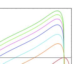
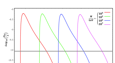
Figure 1: Left: Curves for case (I) [see Table 2], with $M=10^{4}$ GeV, $\delta=+0.378$, $\phi=\phi_{+}=+1.287$ and with different values of $\tan\beta$. Right: Curves for case (II) [see Table 2], with $\tan\beta=15$ GeV, $\delta=-0.378$, $\phi=\phi_{+}=-1.287$ and with different values of $M$. Gray horizontal bands correspond to the experimental value of the baryon asymmetry within the 1-$\sigma$ range given in Eq. (42).

3.3 Renormalizable UV Completion and Consistency Check

Upon building the neutrino mass matrix (26), together with see-saw contribution (24) (emerged via integration of $N_{1,2}$ states) we have used the $d=5$ operator (25). Here we present one renormalizable completion of the model, which gives the latter operator. Also we check the whole construction and show what conditions should be satisfied in order to have fully consistent model without affecting obtained results.

For building fully renormalizable model, we introduce two additional RHN states ${\cal N}$ and $\bar{\cal N}$ with the following superpotential couplings:

$$\lambda l_{1}{\cal N}h_{u}+\bar{\lambda}l_{2}\bar{\cal N}h_{u}-M_{*}{\cal N}\bar{\cal N}~{}.$$ (43)

With these and the couplings of (1)-(3), (22), after removing the phases $x,y,x,\omega,\rho$ in $Y_{\nu}$ (by proper redefinition of the fields) without loss of generality $\bar{\lambda}$ and $M_{*}$ can be taken real and ${\rm arg}(\lambda)={\rm arg}(\bar{m})$. Thus, the full (i.e. ’extended’) Yukawa and RHN matrices will be:

$$\begin{array}[]{ccc}&{\begin{array}[]{cccc}N_{1}&\!N_{2}&\!\!{\cal N}&\!\!\bar{\cal N}\end{array}}\\ \vspace{2mm}Y_{\nu}^{ext}=\begin{array}[]{c}l_{1}\\ l_{2}\\ l_{3}\end{array}\!\!\!\!\!&{\left(\begin{array}[]{cccc}0&0&\lambda&0\\ a_{2}&b_{2}&0&\bar{\lambda}\\ a_{3}&b_{3}e^{i\phi}&0&0\\ \end{array}\right)}~{},\end{array}\!\!~{}~{}~{}~{}~{}\begin{array}[]{ccc}&{\begin{array}[]{cccc}N_{1}&N_{2}&~{}{\cal N}&~{}~{}\bar{\cal N}\end{array}}\\ \vspace{2mm}M_{N}^{ext}=\begin{array}[]{c}N_{1}\\ N_{2}\\ {\cal N}\\ \bar{\cal N}\end{array}\!\!\!\!\!&{\left(\begin{array}[]{cccc}0&M&0&0\\ M&0&0&0\\ 0&0&0&M_{*}\\ 0&0&M_{*}&0\\ \end{array}\right)}~{}.\end{array}\!\!~{}~{}~{}~{}~{}$$ (44)

With these forms, integration of heavy RHN states leads to the neutrino mass matrix

$$M_{\nu}=-v_{u}^{2}Y_{\nu}^{ext}(M_{N}^{ext})^{-1}(Y_{\nu}^{ext})^{T},$$ (45)

which, as desired, indeed has the form of (26) with

$$d_{5}=|\lambda|\bar{\lambda}\frac{|M|}{M_{*}}~{}.$$ (46)

Furthermore, one should make sure that via loops the couplings $\lambda$ and $\bar{\lambda}$ instead of zeros in the textures of Eq. (44) do not induce entries which would affect and/or spoil the results of the neutrino sector and leptogenesis. To check this, one can apply 1-loop RGs for the neutrino Yukawas and RHN masses. Namely, in Eqs. (A.2) and (A.3) with the replacements $Y_{\nu}\to Y_{\nu}^{ext}$, $M_{N}\to M_{N}^{ext}$ we can estimate the 1-loop contributions due to the $\lambda,\bar{\lambda}$ couplings. Since the structure of $Y_{\nu}^{ext}$ may be altered only by the second term at r.h.s of (A.2), we will calculate only contribution due to this type of entry. By the same reason, for the $M_{N}^{ext}$’s correction, we will focus only on the first term (and on it’s transpose) at the r.h.s of Eq. (A.3). Doing so, with an assumption $M_{*}>|M|$, at scale $\mu=M_{*}$ we obtain:

$$\begin{array}[]{ccc}\delta Y_{\nu}^{ext}\approx\!-\frac{3}{16\pi^{2}}\!{\left(\begin{array}[]{cccc}0&0&\lambda|\lambda|^{2}&0\\ a_{2}\bar{\lambda}^{2}&b_{2}\bar{\lambda}^{2}&0&\bar{\lambda}(a_{2}^{2}+b_{2}^{2}+\bar{\lambda}^{2})\\ \times&\times&0&\bar{\lambda}(a_{2}a_{3}+b_{2}b_{3}e^{i\phi})\\ \end{array}\right)\!\!\ln\frac{M_{G}}{M_{*}}}~{},{}{}\end{array}$$

$$\begin{array}[]{ccc}\delta M_{N}^{ext}\approx\!-\frac{1}{8\pi^{2}}\!{\left(\begin{array}[]{cccc}\times&\times&a_{2}\bar{\lambda}M_{*}&b_{2}\bar{\lambda}M\\ \times&\times&b_{2}\bar{\lambda}M_{*}&a_{2}\bar{\lambda}M\\ a_{2}\bar{\lambda}M_{*}&b_{2}\bar{\lambda}M_{*}&0&(|\lambda|^{2}+\bar{\lambda}^{2})M_{*}\\ b_{2}\bar{\lambda}M&a_{2}\bar{\lambda}M&(|\lambda|^{2}+\bar{\lambda}^{2})M_{*}&0\\ \end{array}\right)\!\!\ln\frac{M_{G}}{M_{*}}}~{},\end{array}\!\!~{}~{}~{}~{}~{}$$ (47)

where we have taken into account that at scale $\mu=M_{G}$ the couplings $Y_{\nu}^{ext}$, $M_{N}^{ext}$ have forms given in Eq. (44). In (47) ‘$\times$’ stand for the corrections which do not depend on $\lambda$ and/or $\bar{\lambda}$. Comparing (47) with (44) we see that the structure of $Y_{\nu}^{ext}$ is not changed and $\delta Y_{\nu}^{ext}$ can be negligible for $\lambda,\bar{\lambda}\stackrel{{\scriptstyle<}}{{{}_{\sim}}}\lambda_{\tau}/10$. In fact, from the neutrino sector, we have

$$d_{5}|\bar{m}|=|{\cal A}_{12}|\simeq 1.07\cdot 10^{-11}~{}{\rm GeV}.$$ (48)

[see Eqs. (27) and (36) for definitions.] With this, on the other hand, we have

$$d_{5}\approx 4.15\cdot 10^{-12}\left(\frac{M}{10^{4}{\rm GeV}}\right)\left(\frac{1}{\sin\beta}\right)^{2}\left(\frac{0.85}{r_{\bar{m}}}\right)~{}.$$ (49)

With this and $M_{*}=(3-10)M$, the (46) can be satisfied by the selection

$$|\lambda|\approx\bar{\lambda}=\left(d_{5}\frac{M_{*}}{|M|}\right)^{1/2}\simeq(3.5-6.4)\cdot 10^{-6}\left(\!\frac{M}{10^{4}{\rm GeV}}\!\right)^{\!\!1/2}\!\!\!\left(\frac{1}{\sin\beta}\right)\!\!\left(\frac{0.85}{r_{\bar{m}}}\right)^{\!\!1/2}~{}.$$ (50)

This in turn gives:

$${\rm for}~{}~{}M\stackrel{{\scriptstyle<}}{{{}_{\sim}}}10^{7}~{}{\rm GeV},~{}~{}~{}\tan\beta>1.6~{}~{}\Longrightarrow~{}~{}|\lambda|\approx\bar{\lambda}<3\cdot 10^{-4}~{}.$$ (51)

We checked and made sure that, for such small values of $\lambda,\bar{\lambda}$, the corrections $\delta Y_{\nu}^{ext}$ and $\delta M_{N}^{ext}$ are affecting neither the neutrino sector, nor the leptogenesis. We have also checked that 2-loop corrections are very suppressed too and can be safely ignored. The selection $M_{*}=(3-10)M$ is convenient because the states ${\cal N}$, $\bar{\cal N}$ (having the mass $M_{*}$) decouple earlier than the states $N_{1,2}$ and will not contribute to the leptogenesis process. With all these we conclude that the results obtained in previous subsections stay robust.

Closing this section, we comment (as was also noted in Sect. 2), that throughout our studies we have not attempted to explain and justify texture zeros by symmetries. Our approach here was to consider such textures which give predictive and consistent scenario allowing to calculate cosmological CP violation. The forms of the matrices in Eqs. (3), (22) and/or (44) with specific coupling selections are such that their structures and model’s predictive power (as was demonstrated) are not ruined by radiative corrections. For our purposes this was already satisfactory. More fundamental explanation should be pursued elsewhere.

Acknowledgments

We thank A. Pilaftsis for discussions and helpful comments. The work is partially supported by Shota Rustaveli National Science Foundation (Contract No. DI/12/6-200/13). Z.T. thanks CETUP* (Center for Theoretical Underground Physics and Related Areas) for its hospitality and partial support during 2016 Summer Program. Z.T. also would like to express a special thanks to the Mainz Institute for Theoretical Physics (MITP) for its hospitality and support.

Appendix A Renormalization Group Studies

A.1 Running of $Y_{\nu},Y_{e}$ and $M_{N}$ Matrices and Approximation for $\xi$

RG equations for the charged lepton and neutrino Dirac Yukawa matrices, appearing in the superpotential of Eq. (1), at 1-loop order have the forms [27], [28]:

$$16\pi^{2}\frac{d}{dt}Y_{e}=3Y_{e}Y_{e}^{\dagger}Y_{e}+Y_{\nu}Y_{\nu}^{\dagger}Y_{e}+Y_{e}\left[{\rm tr}\left(3Y_{d}^{\dagger}Y_{d}+Y_{e}^{\dagger}Y_{e}\right)-c_{e}^{a}g_{a}^{2}\right]~{},~{}~{}~{}~{}~{}c_{e}^{a}=(\frac{9}{5},3,0),$$ (A.1)

$$16\pi^{2}\frac{d}{dt}Y_{\nu}=Y_{e}Y_{e}^{\dagger}Y_{\nu}+3Y_{\nu}Y_{\nu}^{\dagger}Y_{\nu}+Y_{\nu}\left[{\rm tr}\left(3Y_{u}^{\dagger}Y_{u}+Y_{\nu}^{\dagger}Y_{\nu}\right)-c_{\nu}^{a}g_{a}^{2}\right]~{},~{}~{}~{}~{}~{}c_{\nu}^{a}=(\frac{3}{5},3,0).$$ (A.2)

$g_{a}=\left(g_{1},g_{2},g_{3}\right)$ denote gauge couplings of $U(1)_{Y},SU(2)_{w}$ and $SU(3)_{c}$ gauge groups respectively. Their 1-loop RG have forms $16\pi^{2}\frac{d}{dt}g_{a}=b_{a}g_{a}^{3}$, with $b_{a}=(\frac{33}{5},1,-3)$, where the hypercharge of $U(1)_{Y}$ is taken in $SU(5)$ normalization.

The RG for the RHN mass matrix at 2-loop level has the form [28]:

$$16\pi^{2}\frac{d}{dt}M_{N}=2M_{N}Y_{\nu}^{{\dagger}}Y_{\nu}-\frac{1}{8\pi^{2}}M_{N}\left[Y_{\nu}^{{\dagger}}Y_{e}Y_{e}^{{\dagger}}Y_{\nu}+Y_{\nu}^{{\dagger}}Y_{\nu}Y_{\nu}^{{\dagger}}Y_{\nu}+Y_{\nu}^{{\dagger}}Y_{\nu}{\,\textup{tr}}(3Y_{u}^{\dagger}Y_{u}+Y_{\nu}^{{\dagger}}Y_{\nu})\right]$$

$$+\frac{1}{8\pi^{2}}M_{N}Y_{\nu}^{{\dagger}}Y_{\nu}\left(\frac{3}{5}g_{1}^{2}+3g_{2}^{2}\right)+({\rm transpose})~{},$$ (A.3)

Let’s start with renormalization of the $Y_{\nu}$’s matrix elements. Ignoring in Eq. (A.2) the ${\cal O}(Y_{\nu}^{3})$ order entries (which are very small because within our studies $|(Y_{\nu})_{ij}|\stackrel{{\scriptstyle<}}{{{}_{\sim}}}10^{-4}$), and from charged fermion Yukawas keeping $\lambda_{\tau}$ and $\lambda_{t}$, we will have:

$$16\pi^{2}\frac{d}{dt}\ln(Y_{\nu})_{ij}\simeq\delta_{i3}\lambda_{\tau}^{2}+3\lambda_{t}^{2}-c_{\nu}^{a}g_{a}^{2}~{}.$$ (A.4)

This gives the solution

$$(Y_{\nu})_{ij}(\mu)=(Y_{\nu G})_{ij}(\eta_{\tau}(\mu))^{\delta_{i3}}\eta_{t}^{3}(\mu)\eta_{g\nu}(\mu),$$ (A.5)

where $Y_{\nu G}$ denotes Yukawa matrix at scale $M_{G}$ and the scale dependent RG factors are given by:

$$\eta_{t,b,\tau}(\mu)\!=\!\exp\!\left(\!\!-\frac{1}{16\pi^{2}}\!\!\int_{t}^{t_{G}}\!\!\lambda^{2}_{t,b,\tau}(t^{\prime})dt^{\prime}\!\right),~{}~{}\eta_{a}(\mu)\!=\!\exp\!\left(\!\!\frac{1}{16\pi^{2}}\!\!\int_{t}^{t_{G}}\!\!\!g^{2}_{a}(t^{\prime})dt^{\prime}\!\right)$$

$$\eta_{g\nu}(\mu)\!=\exp\left(\!\!\frac{1}{16\pi^{2}}\!\int_{t}^{t_{G}}\!\!\!\!c_{\nu}^{a}g^{2}_{a}(t^{\prime})dt^{\prime}\!\!\right)=\eta_{1}^{3/5}(\mu)\eta_{2}^{3}(\mu),~{}~{}~{}{\rm with}~{}~{}~{}t=\ln\mu~{},~{}t^{\prime}=\ln\mu^{\prime}~{},~{}~{}t_{G}=\ln M_{G}.$$ (A.6)

From these, for the combination $Y_{\nu}^{\dagger}Y_{\nu}$ at scale $\mu=M$ we get expression given in Eq. (16).

On the other hand, for the RHN mass splitting and for the phase mismatch [depending on $\xi$ defined in Eq. (17)], the integrals/factors of Eqs. (13), (14), (15) and (16) will be relevant. For obtaining approximate analytical results [for the expression of $\frac{\bar{r}_{\tau}(M)}{r_{\tau}(M)}$] we will use expansions. Namely, we introduce the notation

$${\cal K}=\kappa r_{\tau}\!\left(1-\frac{\lambda^{2}_{\tau}}{16\pi^{2}}\right)$$ (A.7)

and make a Taylor expansion of ${\cal K}(t)$ and $\kappa(t)$ near the point $t=t_{M}$, in powers of $(t-t_{M})$. As will turn out, this will allow to calculate $\xi=\frac{\bar{r}_{\tau}(M)}{r_{\tau}(M)}-1$ in powers of $\frac{\lambda_{\tau}^{2}}{16\pi^{2}}$ [and possibly in powers of other couplings appearing in higher degrees - together with appropriate $\frac{1}{16\pi^{2}}$ factors]. We have:

$${\cal K}(t)={\cal K}(t_{M})+{\cal K}^{\prime}(t_{M})(t-t_{M})+\frac{1}{2}{\cal K}^{\prime\prime}(t_{M})(t-t_{M})^{2}+\cdots$$

$$\kappa(t)=\kappa(t_{M})+\kappa^{\prime}(t_{M})(t-t_{M})+\frac{1}{2}\kappa^{\prime\prime}(t_{M})(t-t_{M})^{2}+\cdots$$ (A.8)

where primes denote derivatives with respect to $t$. Plugging these in Eq. (14) and performing integration we will get:

$$\bar{r}_{\tau}(M)\!=\frac{{\cal K}(t_{M})}{\kappa(t_{M})}\left(\!1+\!\frac{1}{2}\frac{{\cal K}^{\prime}(t_{M})}{{\cal K}(t_{M})}(t_{G}\!-\!t_{M})\!+\!\frac{1}{6}\frac{{\cal K}^{\prime\prime}(t_{M})}{{\cal K}(t_{M})}(t_{G}\!-\!t_{M})^{2}\!+\!\cdots\right)\!\times$$

$$\times\left(\!1+\!\frac{1}{2}\frac{\kappa^{\prime}(t_{M})}{\kappa(t_{M})}(t_{G}\!-\!t_{M})\!+\!\frac{1}{6}\frac{\kappa^{\prime\prime}(t_{M})}{\kappa(t_{M})}(t_{G}\!-\!t_{M})^{2}\!+\!\cdots\right)^{\!-1}\!\!\!\!\!.$$ (A.9)

Using in (A.9) expression (A.7) for ${\cal K}$ and keeping in expansion terms up to the $(t-t_{M})^{2}$, we get

$$\frac{\bar{r}_{\tau}(M)}{r_{\tau}(M)}-1\simeq\frac{1}{2}\left.\frac{r_{\tau}^{\prime}}{r_{\tau}}\right|_{t=t_{M}}\!\!\!\!(t_{G}-t_{M})+\frac{1}{6}\left(\frac{r_{\tau}^{\prime\prime}}{r_{\tau}}+\frac{1}{2}\frac{\kappa^{\prime}r_{\tau}^{\prime}}{\kappa r_{\tau}}\right)_{t=t_{M}}\!\!\!(t_{G}-t_{M})^{2}-\frac{\lambda^{2}_{\tau}(M)}{16\pi^{2}}~{}.$$ (A.10)

As we see, the flavor universal RG factor $\kappa$ drops out at first order of $(t_{G}-t_{M})$. Last term in Eq. (A.10) is due to the 2-loop correction in the RG of $M_{N}$ [in particular $M_{N}Y_{\nu}^{\dagger}Y_{e}Y_{e}^{\dagger}Y_{\nu}$ term of r.h.s of Eq. (A.3)]. Remaining terms are due to 1-loop corrections, proving that cosmological CP violation emerges already at 1-loop level.

Using in (A.10) expressions for the scale factors given in Eqs. (A.6), (15), the RG for $\lambda_{\tau}$ [easily obtained from Eq. (A.1)] and keeping terms up to the order of $\frac{1}{(16\pi^{2})^{2}}$, we obtain the expression for $\xi$ given in Eq. (18).

A.2 Neutrino Mass Matrix Renormalization

In the energy interval $M_{S}\leq\mu<M$ (where $M_{S}$ is the SUSY scale) the RG for the neutrino mass matrix is [29], [28]:

$$M_{S}\leq\mu<M:~{}~{}~{}~{}~{}16\pi^{2}\frac{d}{dt}M_{\nu}=Y_{e}Y_{e}^{\dagger}M_{\nu}+M_{\nu}Y_{e}^{*}Y_{e}^{T}+M_{\nu}\left[6{\rm tr}\left(Y_{u}^{\dagger}Y_{u}\right)-2c_{\nu}^{a}g_{a}^{2}\right].$$ (A.11)

Below the $M_{S}$ scale, effectively we have SM and the RG is [29]:

$$\mu<M_{S}:~{}~{}~{}~{}~{}16\pi^{2}\frac{d}{dt}M_{\nu}=\frac{1}{2}Y_{e}Y_{e}^{\dagger}M_{\nu}+\frac{1}{2}M_{\nu}Y_{e}^{*}Y_{e}^{T}+M_{\nu}\left[{\rm tr}\left(6Y_{u}^{\dagger}Y_{u}\!+\!6Y_{d}^{\dagger}Y_{d}\!+\!2Y_{e}^{\dagger}Y_{e}\right)-3g_{2}^{2}+4\lambda\right]~{},$$ (A.12)

where $\lambda$ is the SM Higgs self-coupling (emerging from the self-interaction term $\lambda(H^{\dagger}H)^{2}$ of the SM Higgs doublet $H$). We will also need the RG evaluation of the VEVs $v_{u}$ and $v$, which in appropriate energy intervals are given by [30, 31, 32, 33]:

$$\mu>M_{S}:~{}~{}~{}~{}~{}~{}~{}~{}16\pi^{2}\frac{d}{dt}v_{u}=v_{u}\left(-3\lambda_{t}^{2}+\frac{1}{4}c_{\nu}^{a}g_{a}^{2}\right),~{}$$ (A.13)

$$\mu<M_{S}:~{}~{}~{}~{}~{}16\pi^{2}\frac{d}{dt}v=v\left(-3\lambda_{t}^{2}-3\lambda_{b}^{2}-\lambda_{\tau}^{2}+\frac{3}{4}c_{\nu}^{a}g_{a}^{2}\right).$$ (A.14)

At scale $M$, after decoupling of the RHN states, the neutrino mass matrix is formed with the form:

$$M_{\nu}^{ij}(M)=\left(\begin{array}[]{ccc}\times&\times&\times\\ \times&\times&\times\\ \times&\times&\times\\ \end{array}\right)\frac{v_{u}^{2}(M)}{M}~{},$$ (A.15)

where ‘$\times$’ stand for entries depending on Yukawa couplings. After renormalization, keeping $\lambda_{\tau},\lambda_{t}$ and $g_{a}$ in the above RGs, for the neutrino mass matrix at scale $M_{Z}$ we obtain:

$$M_{\nu}^{ij}(M_{Z})=\left(\begin{array}[]{ccc}\times&\times&(\times)\!\cdot\!r_{\nu 3}\\ \times&\times&(\times)\!\cdot\!r_{\nu 3}\\ (\times)\!\cdot\!r_{\nu 3}&(\times)\!\cdot\!r_{\nu 3}&(\times)\!\cdot\!r_{\nu 3}^{2}\\ \end{array}\right)\bar{m}~{},~{}~{}~{}~{}{\rm with}~{}~{}~{}~{}~{}\bar{m}=\frac{v^{2}(M_{Z})s^{2}_{\beta}}{M}r_{\bar{m}}~{},$$ (A.16)

where ‘$\times$’ denotes entries determined at scale $M$ corresponding to those in (A.15), and RG factors are given by

$$r_{\nu 3}\!=\!\left(\!\frac{\eta_{\tau}(t_{Z})}{\eta_{\tau}(t_{M_{S}})}\!\right)^{1/2}\!\left(\!\frac{\eta_{\tau}(t_{M_{S}})}{\eta_{\tau}(t_{M})}\!\right)~{},$$ (A.17)

$$r_{\bar{m}}\!=\eta_{\lambda}^{4}\!\left(\!\frac{\eta_{t}(t_{m_{t}})}{\eta_{t}(t_{M})}\!\right)^{12}\!\!\left(\!\frac{\eta_{b}(t_{Z})}{\eta_{b}(t_{M_{S}})}\!\right)^{12}\!\!\left(\!\frac{\eta_{\tau}(t_{Z})}{\eta_{\tau}(t_{M_{S}})}\!\right)^{4}\!\!\left(\!\frac{\eta_{2}(t_{Z})}{\eta_{2}(t_{M})}\!\right)^{\!\frac{15}{2}}\!\!\left(\!\frac{\eta_{1}^{3/5}(t_{Z})\eta_{1}^{2/5}(t_{M_{S}})}{\eta_{1}(t_{M})}\!\right)^{\!\frac{3}{2}}~{},$$ (A.18)

where

$$\eta_{\lambda}=\exp\left(-\frac{1}{16\pi^{2}}\int_{t_{m_{h}}}^{t_{M_{S}}}\lambda(t)dt\right)~{},$$ (A.19)

and remaining $\eta$-factors are defined in Eq. (A.6).

We will also need the RG factor relating the VEV $v_{u}(M)$ to the $v(M_{Z})$. Using Eqs. (A.13) and (A.14) we obtain:

$$r_{v_{u}}\!=\!\frac{v_{u}(M)}{v(M_{Z})s_{\beta}}\!=\!\left(\!\frac{\eta_{t}(t_{m_{t}})}{\eta_{t}(t_{M})}\!\right)^{3}\!\!\left(\!\frac{\eta_{b}(t_{Z})}{\eta_{b}(t_{M_{S}})}\!\right)^{3}\!\!\left(\!\frac{\eta_{\tau}(t_{Z})}{\eta_{\tau}(t_{M_{S}})}\!\right)\!\!\left(\!\frac{\eta_{2}^{3}(t_{Z})\eta_{2}^{-2}(t_{M_{S}})}{\eta_{2}(t_{M})}\!\right)^{\!\frac{3}{4}}\!\!\left(\!\frac{\eta_{1}^{3}(t_{Z})\eta_{1}^{-2}(t_{M_{S}})}{\eta_{1}(t_{M})}\!\right)^{\!\frac{3}{20}}~{}.$$ (A.20)

A.3 Boundary and Matching Conditions

For finding the RG factors, appearing in the baryon asymmetry, we numerically solve renormalization group equations from the scale $M_{Z}$ up to the $M_{G}\simeq 2\cdot 10^{16}$ GeV scale. For simplicity, for all SUSY particle masses we take common mass scale $M_{S}$. Thus, in the energy interval $M_{Z}\leq\mu<M_{S}$, the Standard Model RGs for $\overline{\rm MS}$ coupling constants are used. However, in the interval $M_{S}\leq\mu\leq M_{G}$, since we are dealing with the SUSY, the RGs for the $\overline{\rm DR}$ couplings are applied. Below we give boundary and matching conditions for the gauge couplings $g_{1,2,3}$, for Yukawa constant $\lambda_{t,b,\tau}$ and for the Higgs self-coupling $\lambda$.

Gauge couplings

We choose our inputs for the $\overline{\rm MS}$ gauge couplings at scale $M_{Z}$ as follows:

$$\alpha_{1}^{-1}(M_{Z})=\frac{3}{5}c_{w}^{2}\alpha_{em}^{-1}(M_{Z})+\frac{3}{5}c_{w}^{2}\frac{8}{9\pi}\ln\frac{m_{t}}{M_{Z}}~{},~{}~{}~{}~{}~{}\alpha_{2}^{-1}(M_{Z})=s_{w}^{2}\alpha_{em}^{-1}(M_{Z})+s_{w}^{2}\frac{8}{9\pi}\ln\frac{m_{t}}{M_{Z}}~{},$$

$$\alpha_{3}^{-1}(M_{Z})=\alpha_{s}^{-1}(M_{Z})+\frac{1}{3\pi}\ln\frac{m_{t}}{M_{Z}}~{},$$ (A.21)

where logarithmic terms $\ln\frac{m_{t}}{M_{Z}}$ are due to the top quark threshold correction [34], [32]. Taking $\alpha_{s}(M_{Z})=0.1185$, $\alpha_{em}^{-1}(M_{Z})=127.934$ and $s_{w}^{2}=0.2313$, from (A.21) we obtain:

$$\alpha_{1}^{-1}(M_{Z})=59.0057+\frac{8c_{w}^{2}}{15\pi}\ln\frac{m_{t}}{M_{Z}}~{},~{}~{}~{}\alpha_{2}^{-1}(M_{Z})=29.5911+\frac{8s_{w}^{2}}{9\pi}\ln\frac{m_{t}}{M_{Z}}~{},$$

$$\alpha_{3}^{-1}(M_{Z})=8.4388+\frac{1}{3\pi}\ln\frac{m_{t}}{M_{Z}}~{}.$$ (A.22)

With these inputs we run $g_{1,2,3}$ via the 2-loop RGs from $M_{Z}$ up to the scale $M_{S}$.

At scale $\mu=M_{S}$ we use the matching conditions between $\overline{\rm DR}-\overline{\rm MS}$ gauge couplings [35, 36]:

$${\rm at}~{}\mu=M_{S}:~{}~{}~{}\frac{1}{\alpha_{1}^{\rm\overline{DR}}}=\frac{1}{\alpha_{1}^{\rm\overline{MS}}}~{},~{}~{}~{}~{}\frac{1}{\alpha_{2}^{\rm\overline{DR}}}=\frac{1}{\alpha_{2}^{\rm\overline{MS}}}-\frac{1}{6\pi}~{},~{}~{}~{}~{}\frac{1}{\alpha_{3}^{\rm\overline{DR}}}=\frac{1}{\alpha_{3}^{\rm\overline{MS}}}-\frac{1}{4\pi}~{}.$$ (A.23)

Above the scale $M_{S}$ we apply 2-loop SUSY RG equations in $\overline{\rm DR}$ scheme [27].

Yukawa Couplings and $\lambda$

At the scale $M_{S}$ all SUSY states decouple and we are left with the Standard Model with one Higgs doublet. Thus, the third family Yukawa couplings and the self-coupling are determined as:

$$\lambda_{t}(m_{t})=\frac{m_{t}(m_{t})}{v(m_{t})}~{},~{}~{}~{}~{}\lambda_{b}(M_{Z})=\frac{2.89{\rm GeV}}{v(M_{Z})}~{},~{}~{}~{}~{}\lambda_{\tau}(M_{Z})=\frac{1.746{\rm GeV}}{v(M_{Z})}~{},~{}~{}~{}$$

$$\lambda(m_{h})=\frac{1}{4}\left(\frac{m_{h}}{v(m_{h})}\right)^{2},~{}~{}~{}~{}~{}{\rm with}~{}~{}~{}v(M_{Z})=174.1~{}{\rm GeV}~{},~{}~{}~{}m_{h}=125.15~{}{\rm GeV}~{},$$ (A.24)

where $m_{t}(m_{t})$ is the top quark running mass related to the pole mass as:

$$m_{t}(m_{t})=p_{t}M_{t}^{pole}~{}.$$ (A.25)

The factor $p_{t}$ is $p_{t}\simeq 1/1.0603$ [37], while the recent measured value of the top’s pole mass is [38]:

$$M_{t}^{pole}=(173.34\pm 0.76)~{}{\rm GeV}.$$ (A.26)

We take the values of (A.24) as boundary conditions for solving 2-loop RG equations [39], [32] for $\lambda_{t,b,\tau}$ and $\lambda$ from the $M_{Z}$ scale up to the scale $M_{S}$.

Above the $M_{S}$ scale, we have MSSM states including two doublets $h_{u}$ and $h_{d}$, which couple with up type quarks and down type quarks and charged leptons respectively. Thus, the third family Yukawa couplings at $M_{S}$ are $\approx\lambda_{t}(M_{S})/s_{\beta},\lambda_{b}(M_{S})/c_{\beta}$ and $\lambda_{\tau}(M_{S})/c_{\beta}$, with $s_{\beta}\equiv\sin\beta,c_{\beta}\equiv\cos\beta$. Above the scale $M_{S}$ we apply 2-loop SUSY RG equations in $\overline{\rm DR}$ scheme [27]. Thus, at $\mu=M_{S}$ we use the matching conditions between $\overline{\rm DR}-\overline{\rm MS}$ couplings:

$${\rm at}~{}\mu=M_{S}:~{}~{}~{}~{}~{}~{}~{}~{}~{}~{}~{}~{}~{}~{}\lambda_{t}^{\rm\overline{DR}}\simeq\frac{\lambda_{t}^{\rm\overline{MS}}}{s_{\beta}}\left[1+\frac{1}{16\pi^{2}}\left(\frac{g_{1}^{2}}{120}+\frac{3g_{2}^{2}}{8}-\frac{4g_{3}^{2}}{3}\right)\right],$$

$$\lambda_{b}^{\rm\overline{DR}}\simeq\frac{\lambda_{b}^{\rm\overline{MS}}}{c_{\beta}}\left[1\!+\!\frac{1}{16\pi^{2}}\left(\frac{13g_{1}^{2}}{120}+\frac{3g_{2}^{2}}{8}-\frac{4g_{3}^{2}}{3}\right)\right],~{}~{}~{}~{}\lambda_{\tau}^{\rm\overline{DR}}\simeq\frac{\lambda_{\tau}^{\rm\overline{MS}}}{c_{\beta}}\left[1\!+\!\frac{1}{16\pi^{2}}\left(-\frac{9g_{1}^{2}}{40}+\frac{3g_{2}^{2}}{8}\right)\right],$$ (A.27)

where expressions in brackets of r.h.s of the relations are due to the $\overline{\rm DR}-\overline{\rm MS}$ conversions [36]. With Eq. (A.27)’s matchings we run corresponding couplings from the scale $M_{S}$ up to the $M_{G}$ scale. Throughout the paper, above the mass scale $M_{S}$ without using the superscript $\overline{\rm DR}$ we assume the couplings determined in this scheme.

Appendix B Contribution to the Baryon Asymmetry from $\tilde{N}$ Decays

Impact of the decays of the right handed sneutrinos - the scalar partners of the RHNs - was estimated in [11] for specific textures. Here we give more detailed investigation and give results for the neutrino model discussed in Sect. 3.1.

We will need to derive masses of the RH sneutrinos and their couplings to the components of the superfields $l$ and $h_{u}$. For this purpose, we should include the soft breaking terms

$$V_{SB}^{\nu}=\tilde{l}^{T}A_{\nu}\tilde{N}h_{u}-\frac{1}{2}\tilde{N}^{T}B_{N}\tilde{N}+{\rm h.c.}+\tilde{l}^{{\dagger}}m^{2}_{\tilde{l}}\tilde{l}+\tilde{N}^{{\dagger}}m^{2}_{\tilde{N}}\tilde{N}~{},$$ (B.1)

which, together with the superpotential couplings, will be relevant. As it turns out, relevant will be $A_{\nu}$ and $B_{N}$ couplings. Therefore, first we will study their renormalization. After this, we investigate masses of the physical RH sneutrinos and their couplings to the lepton superfield components. These, at the end, will be used for the calculation of the contribution in the baryon asymmetry via the RH sneutrino decay processes.

B.1 Renormalization of Soft $A_{\nu}$ and $B_{N}$ Terms

From general expressions of Ref. [27] we can derive RGs for $A_{\nu}$ and $B_{N}$, which at 1-loop level have the forms:

$$16\pi^{2}\frac{d}{dt}A_{\nu}=Y_{e}Y_{e}^{\dagger}A_{\nu}+2\hat{A}_{e}Y_{e}^{\dagger}Y_{\nu}+5Y_{\nu}Y_{\nu}^{\dagger}A_{\nu}\!+\!A_{\nu}\!\left[{\rm tr}(3Y_{u}^{\dagger}Y_{u}+Y_{\nu}^{\dagger}Y_{\nu})+4Y_{\nu}^{\dagger}Y_{\nu}-c_{\nu}^{a}g_{a}^{2}\right]$$

$$+2Y_{\nu}\!\left[{\rm tr}(3Y_{u}^{\dagger}\hat{A}_{u}+Y_{\nu}^{\dagger}A_{\nu})+c_{\nu}^{a}g_{a}^{2}M_{\tilde{V}_{a}}\right]~{},$$ (B.2)

$$16\pi^{2}\frac{d}{dt}B_{N}=2B_{N}Y_{\nu}^{\dagger}Y_{\nu}+2Y_{\nu}^{T}Y_{\nu}^{*}B_{N}+4M_{N}Y_{\nu}^{\dagger}A_{\nu}+4A_{\nu}^{T}Y_{\nu}^{*}M_{N}~{}.$$ (B.3)

Note that, applying these expressions for the third generation states we can get expressions of [40] (see Eqs. (17) and (55) of this Ref., which uses slightly different definitions for the couplings). These results are also compatible with those given in [41] (with replacements $Y\to Y^{T}$, $A\to A^{T}$).

We parameterize the matrix $B_{N}$ as

$$B_{N}=(M_{N})_{12}m_{B}\left(\begin{array}[]{cc}\delta_{BN}^{(1)}&1\\ 1&\delta_{BN}^{(2)}\\ \end{array}\right),$$ (B.4)

where all entries $(M_{N})_{12},m_{B}$, $\delta_{BN}^{(1,2)}$ run and their RGs can be derived from the RG equations given above. For the matrix $A_{\nu}$, let’s use the parametrization

$$A_{\nu}=m_{A}a_{\nu}~{},$$ (B.5)

where $m_{A}$ is a constant and the elements of the $a_{\nu}$ matrix run. The matrix $\hat{A}_{e}$ is

$$\hat{A}_{e}={\rm Diag}\left(A_{e},A_{\mu},A_{\tau}\right)$$ (B.6)

(similar to the structure of $Y_{e}$ Yukawa matrix). We will use the following boundary conditions:

$${\rm at}~{}\mu=M_{G}:~{}~{}~{}~{}a_{\nu}=Y_{\nu}~{},~{}~{}~{}~{}\delta_{BN}^{(1)}=\delta_{BN}^{(2)}=0,~{}~{}~{}\hat{A}_{e}=m_{A}{\rm Diag}\left(\lambda_{e},\lambda_{\mu},\lambda_{\tau}\right)$$

$$\hat{A}_{u}=m_{A}Y_{uG}~{},~{}~{}~{}~{}\hat{A}_{d}=m_{A}Y_{dG}~{},$$ (B.7)

which assume proportionality (alignment) of the soft SUSY breaking terms with the corresponding superpotential couplings.

With (B.4), (B.5), using (B.3) we have:

$$16\pi^{2}\frac{d}{dt}\delta_{BN}^{(1)}\simeq 4(Y_{\nu}^{\dagger}Y_{\nu})_{21}+8\frac{m_{A}}{m_{B}}(Y_{\nu}^{\dagger}a_{\nu})_{21}~{},~{}~{}~{}~{}16\pi^{2}\frac{d}{dt}\delta_{BN}^{(2)}\simeq 4(Y_{\nu}^{\dagger}Y_{\nu})_{12}+8\frac{m_{A}}{m_{B}}(Y_{\nu}^{\dagger}a_{\nu})_{12}.$$ (B.8)

Due to RG effects, the alignment between $Y_{\nu}$ and $a_{\nu}$ (which holds at the GUT scale) is violated. In particular:

$$16\pi^{2}\frac{d}{dt}\left(\frac{(a_{\nu})_{ij}}{(Y_{\nu})_{ij}}\right)\simeq 2\delta_{i3}\frac{\lambda_{\tau}A_{\tau}}{m_{A}}+\frac{2}{m_{A}}(3\lambda_{t}A_{t}+c_{\nu}^{a}g_{a}^{2}M_{\tilde{V}_{a}})~{},$$ (B.9)

where at r.h.s. we kept third family couplings, gauge couplings and gaugino masses. From this we derive

$$a_{\nu}\simeq\left(\begin{array}[]{ccc}1+\epsilon_{0}&0&0\\ 0&1+\epsilon_{0}&0\\ 0&0&1+\epsilon_{0}+\epsilon\\ \end{array}\right)\!Y_{\nu}$$

$${\rm with}~{}~{}~{}\epsilon_{0}=-\frac{1}{8\pi^{2}m_{A}}\int_{t}^{t_{G}}\!\!\!\!dt(3\lambda_{t}A_{t}+c_{\nu}^{a}g_{a}^{2}M_{\tilde{V}_{a}})~{},~{}~{}~{}~{}~{}~{}\epsilon=-\frac{1}{8\pi^{2}m_{A}}\int_{t}^{t_{G}}\!\!\!\!dt\lambda_{\tau}A_{\tau}~{}.$$ (B.10)

Using (B.10) in Eqs. (B.8) and (B.4) we obtain

$${\rm at}~{}\mu=M:~{}~{}~{}~{}B_{N}=m_{B}M\left(\begin{array}[]{cc}-\alpha\delta_{N}(1+\bar{\epsilon}_{1})&1\\ 1&-\alpha\delta_{N}^{*}(1+\bar{\epsilon}_{2})\\ \end{array}\right),~{}~{}~{}~{}\alpha=1+2\frac{m_{A}}{m_{B}}~{}$$ (B.11)

and

$$\bar{\epsilon}_{1}\!=\!\frac{1}{4\pi^{2}\alpha\delta_{N}}\!\int_{t_{M}}^{t_{G}}\!\!dt\!\left(\!\!Y_{\nu}^{\dagger}(\frac{\alpha}{16\pi^{2}}Y_{e}Y_{e}^{\dagger}+2\frac{m_{A}}{m_{B}}\hat{\epsilon})Y_{\nu}\!\right)_{\!\!21}\!,~{}~{}~{}\bar{\epsilon}_{2}\!=\!\frac{1}{4\pi^{2}\alpha\delta_{N}^{*}}\!\int_{t_{M}}^{t_{G}}\!\!dt\!\left(\!\!Y_{\nu}^{\dagger}(\frac{\alpha^{*}}{16\pi^{2}}Y_{e}Y_{e}^{\dagger}+2\frac{m_{A}^{*}}{m_{B}^{*}}\hat{\epsilon}^{*})Y_{\nu}\!\right)_{\!\!21}^{\!\!*}~{},~{}$$

$${\rm with}~{}~{}~{}~{}\hat{\epsilon}={\rm Diag}\left(\epsilon_{0},~{}\epsilon_{0},~{}\epsilon_{0}+\epsilon\right).$$ (B.12)

The form of $B_{N}$ given in Eq. (B.11) will be needed to construct the sneutrino mass matrix, which we will do below.

B.2 Sneutrino Mass Matrix and its Diagonalization

For calculating scalar RHN masses, from (B.1) we keep only $B_{N}$-term. Also include the mass² term $\tilde{N}^{\dagger}M_{N}^{\dagger}M_{N}\tilde{N}$ coming from the superpotential. Therefore, we consider the following quadratic potential:

$$V_{\tilde{N}}^{(2)}=\tilde{N}^{\dagger}M_{N}^{\dagger}M_{N}\tilde{N}-\left(\frac{1}{2}\tilde{N}^{T}B_{N}\tilde{N}+{\rm h.c.}\right)~{}.$$ (B.13)

With the transformation of the $N$ superfields $N=U_{N}N^{\prime}$ (according to Eq. (6), the $U_{N}$ diagonalizes the fermionic RHN mass matrix), we obtain:

$$V_{\tilde{N}}^{(2)}=\tilde{N}^{\hskip 1.42262pt{}^{\prime}\!{\dagger}}(M_{N}^{Diag})^{2}\tilde{N}^{\prime}-\left(\frac{1}{2}\tilde{N}^{\hskip 1.42262pt{}^{\prime}T}U_{N}^{T}B_{N}U_{N}\tilde{N}^{\prime}+{\rm h.c.}\right)~{}.$$ (B.14)

On the other hand, from (B.11) we have

$$U_{N}^{T}B_{N}U_{N}=m_{B}|M|\left(\begin{array}[]{cc}1-\tilde{\alpha}|\delta_{N}|&\frac{i}{2}\alpha|\delta_{N}|(\bar{\epsilon}_{1}-\bar{\epsilon}_{2})\\ \frac{i}{2}\alpha|\delta_{N}|(\bar{\epsilon}_{1}-\bar{\epsilon}_{2})&1+\tilde{\alpha}|\delta_{N}|\\ \end{array}\right),~{}~{}~{}{\rm with}~{}~{}~{}~{}\tilde{\alpha}=\alpha(1+\frac{\bar{\epsilon}_{1}+\bar{\epsilon}_{2}}{2})~{}.$$ (B.15)

With further phase redefinition

$$\tilde{N}^{\prime}=\tilde{P}_{1}\tilde{N}^{\prime\prime}~{},~{}~{}~{}~{}~{}\tilde{P}_{1}={\rm Diag}\left(e^{-i\tilde{\omega}_{1}/2},e^{-i\tilde{\omega}_{2}/2}\right)~{},~{}~{}~{}~{}~{}{\rm with}~{}~{}~{}\tilde{\omega}_{1,2}={\rm Arg}[m_{B}(1\mp\tilde{\alpha}|\delta_{N}|)]$$ (B.16)

and by going to the real scalar components

$${\tilde{N}_{1}}^{\prime\prime}=\frac{1}{\sqrt{2}}(\tilde{N}_{1}^{R}+i\tilde{N}_{1}^{I})~{},~{}~{}~{}~{}~{}{\tilde{N}_{2}}^{\prime\prime}=\frac{1}{\sqrt{2}}(\tilde{N}_{2}^{R}+i\tilde{N}_{2}^{I})~{},$$ (B.17)

we will have

$$-\left(\frac{1}{2}\tilde{N}^{\hskip 1.42262pt{}^{\prime}T}U_{N}^{T}B_{N}U_{N}\tilde{N}^{\prime}+{\rm h.c.}\right)=-\frac{|Mm_{B}|}{2}\left|1-\tilde{\alpha}|\delta_{N}|\right|\left(\!(\tilde{N}_{1}^{R})^{2}-(\tilde{N}_{1}^{I})^{2}\!\right)$$

$$-\frac{|Mm_{B}|}{2}\left|1+\tilde{\alpha}|\delta_{N}|\right|\left(\!(\tilde{N}_{2}^{R})^{2}-(\tilde{N}_{2}^{I})^{2}\!\right)-|M|{\rm Re}(m_{B}\delta_{\epsilon})\left(\tilde{N}_{1}^{R}\tilde{N}_{2}^{R}-\tilde{N}_{1}^{I}\tilde{N}_{2}^{I}\right)+|M|{\rm Im}(m_{B}\delta_{\epsilon})\left(\tilde{N}_{1}^{I}\tilde{N}_{2}^{R}+\tilde{N}_{1}^{R}\tilde{N}_{2}^{I}\right)$$

$${\rm with}~{}~{}~{}~{}\delta_{\epsilon}=i\alpha|\delta_{N}|\frac{\bar{\epsilon}_{1}-\bar{\epsilon}_{2}}{2}e^{-i(\tilde{\omega}_{1}+\tilde{\omega}_{2})/2}~{}.$$ (B.18)

From (B.14) and (B.18) we obtain the mass² terms:

$$V_{\tilde{N}}^{(2)}=\frac{1}{2}\tilde{n}^{0T}M_{\tilde{n}}^{2}\tilde{n}^{0}~{},~{}~{}~{}~{}{\rm with}~{}~{}~{}~{}\tilde{n}^{0T}=\left(\tilde{N}_{1}^{R},\tilde{N}_{1}^{I},\tilde{N}_{2}^{R},\tilde{N}_{2}^{I}\right)~{}$$ (B.19)

and

$$M_{\tilde{n}}^{2}=\left(\begin{array}[]{cccc}(\tilde{M}_{1}^{0})^{2}&0&-|M|{\rm Re}(m_{B}\delta_{\epsilon})&|M|{\rm Im}(m_{B}\delta_{\epsilon})\\ 0&(\tilde{M}_{2}^{0})^{2}&|M|{\rm Im}(m_{B}\delta_{\epsilon})&|M|{\rm Re}(m_{B}\delta_{\epsilon})\\ -|M|{\rm Re}(m_{B}\delta_{\epsilon})&|M|{\rm Im}(m_{B}\delta_{\epsilon})&(\tilde{M}_{3}^{0})^{2}&0\\ |M|{\rm Im}(m_{B}\delta_{\epsilon})&|M|{\rm Re}(m_{B}\delta_{\epsilon})&0&(\tilde{M}_{4}^{0})^{2}\\ \end{array}\right)$$ (B.20)

where

$$(\tilde{M}_{1}^{0})^{2}=|M|^{2}(1-|\delta_{N}|)^{2}-|m_{B}M|\left|1-\tilde{\alpha}|\delta_{N}|\right|,~{}~{}(\tilde{M}_{2}^{0})^{2}=|M|^{2}(1-|\delta_{N}|)^{2}+|m_{B}M|\left|1-\tilde{\alpha}|\delta_{N}|\right|~{},$$

$$(\tilde{M}_{3}^{0})^{2}=|M|^{2}(1+|\delta_{N}|)^{2}-|m_{B}M|\left|1+\tilde{\alpha}|\delta_{N}|\right|,~{}~{}(\tilde{M}_{4}^{0})^{2}=|M|^{2}(1+|\delta_{N}|)^{2}+|m_{B}M|\left|1+\tilde{\alpha}|\delta_{N}|\right|$$ (B.21)

The coupling of $\tilde{n}^{0}$ states with the fermions emerges from the $F$-term of the superpotential $l^{T}Y_{\nu}Nh_{u}$. Following the transformations, indicated above, we will have:

$$(l^{T}Y_{\nu}Nh_{u})_{F}\to\tilde{h}_{u}l^{T}Y_{\nu}\tilde{N}=e^{-i\tilde{\omega}_{2}/2}\tilde{h}_{u}l^{T}Y_{\nu}U_{N}\left(\rho_{u}e^{i(\tilde{\omega}_{2}-\tilde{\omega}_{1})/2},\rho_{d}\right)\tilde{n}^{0}~{},$$

$${\rm with}~{}~{}~{}\rho_{u}=\frac{1}{\sqrt{2}}\left(\begin{array}[]{cc}1&i\\ 0&0\end{array}\right)~{},~{}~{}~{}\rho_{d}=\frac{1}{\sqrt{2}}\left(\begin{array}[]{cc}0&0\\ 1&i\end{array}\right)~{}.$$ (B.22)

Performing the diagonalization of the matrix (B.20) by the transformation $V_{\tilde{n}}^{T}M_{\tilde{n}}^{2}V_{\tilde{n}}=(M_{\tilde{n}}^{Diag})^{2}$, $\tilde{n}^{0}=V_{\tilde{n}}\tilde{n}$, the fermion coupling with the scalar $\tilde{n}$ eigenstates will be

$$\tilde{h}_{u}l^{T}Y_{F}\tilde{n}~{}~{}~{}~{}~{}~{}{\rm with}~{}~{}~{}Y_{F}=Y_{\nu}\tilde{V}^{0}V_{\tilde{n}}~{},~{}~{}~{}\tilde{V}^{0}=U_{N}\left(\rho_{u}e^{-i\tilde{\omega}_{1}/2},\rho_{d}e^{-i\tilde{\omega}_{2}/2}\right)~{}.$$ (B.23)

The coupling with the slepton $\tilde{l}$ is derived from the interaction term $h_{u}\tilde{l}^{T}\left(Y_{\nu}M_{N}^{*}\tilde{N}^{*}-A_{\nu}\tilde{N}\right)$. Going from $\tilde{N}$ to the $\tilde{n}$ states, we obtain

$$h_{u}\tilde{l}^{T}Y_{B}\tilde{n}~{}~{}~{}~{}{\rm with}~{}~{}~{}Y_{B}=(Y_{\nu}M_{N}^{*}\tilde{V}^{0*}-A_{\nu}\tilde{V}^{0})V_{\tilde{n}}~{}.$$ (B.24)

For a given values of $M,m_{B}$ and $m_{A}$, with help of Eqs. (B.20), (B.23) and (B.24), we will have coupling matrices $Y_{F}$, $Y_{B}$ and all other quantities needed for calculation of the baryon asymmetry created via the decays of the $\tilde{n}_{1,2,3,4}$ states.

B.3 Asymmetry Via $\tilde{n}$ Decays

Now we are ready to discuss the contribution to the net baryon asymmetry from the out of equilibrium resonant decays of the right handed sneutrinos (RHS). As we have seen, with SUSY breaking terms, the masses of RHS’s differ from their fermionic partners’ masses. Thus we have mass-eigenstate RHS’s $\tilde{n}_{i=1,2,3,4}$ with masses $\tilde{M}_{i=1,2,3,4}$ respectively. With the SUSY scale $M_{S}$ smaller (at least by a factor of 3) than the scale $M$, the states $\tilde{n}_{i}$ remain nearly degenerate.

For the resonant $\tilde{n}$-decays we will apply resummed effective amplitude technique [17]. Effective amplitudes for the real $\tilde{n}_{i}$ decay, say into the lepton $l_{\alpha}$ ($\alpha=1,2,3$) and antilepton $\overline{l}_{\alpha}$ respectively are given by [17]

$$\hat{S}_{\alpha i}=S_{\alpha i}-\sum_{j}S_{\alpha j}\frac{\Pi_{ji}(\tilde{M}_{i})(1-\delta_{ij})}{\tilde{M}_{i}^{2}-\tilde{M}_{j}^{2}+\Pi_{jj}(\tilde{M}_{i})}~{},~{}~{}\hat{\overline{S}}_{\alpha i}=S_{\alpha i}^{*}-\sum_{j}S_{\alpha j}^{*}\frac{\Pi_{ji}(\tilde{M}_{i})(1-\delta_{ij})}{\tilde{M}_{i}^{2}-\tilde{M}_{j}^{2}+\Pi_{jj}(\tilde{M}_{i})}~{},$$ (B.25)

where $S_{\alpha i}$ is a tree level amplitude and $\Pi_{ij}$ is a two point Green function’s (polarization operator of $\tilde{n}_{i}-\tilde{n}_{j}$) absorptive part. The CP asymmetry is then given by

$$\epsilon_{i}^{sc}=\frac{\sum_{\alpha}\left(|\hat{S}_{\alpha i}|^{2}-|\hat{\overline{S}}_{\alpha i}|^{2}\right)}{\sum_{\alpha}\left(|\hat{S}_{\alpha i}|^{2}+|\hat{\overline{S}}_{\alpha i}|^{2}\right)}~{}.$$ (B.26)

With $Y_{F}$ and $Y_{B}$ given by Eq. (B.23) and (B.24) we can calculate polarization diagram’s (with external legs $\tilde{n}_{i}$ and $\tilde{n}_{j}$) absorptive part $\Pi_{ij}$, which at the 1-loop level is given by:

$$\Pi_{ij}(p)=\frac{i}{8\pi}\left(p^{2}Y_{F}^{\dagger}Y_{F}+p^{2}Y_{F}^{T}Y_{F}^{*}+Y_{B}^{\dagger}Y_{B}+Y_{B}^{T}Y_{B}^{*}\right)_{ij}~{},$$ (B.27)

where $p$ denotes external momentum in the diagram and upon evaluation of (B.26), for $\Pi$ we should use (B.27) with $p=\tilde{M}_{i}$.

​$(m_{A},m_{B})=(100~{}\!i,500){\rm GeV}$​

​$(m_{A},m_{B})\!=\!(500,1000){\rm GeV}$ ​

$$\begin{array}[]{|c|c|c|c|c|}\hline\cr\vspace{-0.3cm}\hfil&&&&\\ {\rm Case}&~{}~{}~{}10^{4}\!\times\!a_{2}{}{}{}{}&~{}~{}~{}10^{11}\!\times\!\frac{\tilde{n}_{b}}{s}{}{}{}&~{}~{}~{}10^{4}\!\times\!a_{2}{}{}{}{}&~{}~{}~{}10^{11}\!\times\!\frac{\tilde{n}_{b}}{s}{}{}{}\\ \hline\cr{\bf(I_{-})}&0.016&0.25&0.016&0.24\\ \hline\cr{\bf(I.1)}&0.0159785&0.25&0.0159785&0.25\\ \hline\cr{\bf(I.2)}&0.0299&0.24&0.0299&0.24\\ \hline\cr{\bf(I.3)}&0.0987&0.24&0.0987&0.24\\ \hline\cr{\bf(I.4)}&0.3237&0.24&0.3237&0.24\\ \hline\cr{\bf(I.5)}&1.05655&0.23&1.05655&0.23\\ \hline\cr\hline\cr{\bf(II_{-})}&0.0229&0.25&0.0229&0.24\\ \hline\cr{\bf(II.1)}&0.0229&0.25&0.0229&0.24\\ \hline\cr{\bf(II.2)}&0.02986&0.24&0.02986&0.24\\ \hline\cr{\bf(II.3)}&0.09835&0.24&0.09835&0.24\\ \hline\cr{\bf(II.4)}&0.322&0.24&0.322&0.24\\ \hline\cr{\bf(II.5)}&1.05&0.23&1.05&0.23\\ \hline\cr\end{array}$$

Table 4: Values of $\frac{\Delta n_{b}}{s}=\frac{\tilde{n}_{b}}{s}$ - contributions to the Baryon asymmetry via decays of the right handed sneutrinos for cases given in table 3 (i.e. for values of $a_{2}$ giving $\left(\frac{n_{b}}{s}\!\right)_{\rm max}$ given in Tab. 3). These values correspond to the phases $\delta=-0.378$ and $\phi_{+}=-1.287$.

In an unbroken SUSY limit, neglecting finite temperature effects ($T\to 0$), the $\tilde{N}$ decay does not produce lepton asymmetry due to the following reason. The decays of $\tilde{N}$ in the fermion and scalar channels are respectivelly $\tilde{N}\to l\tilde{h}_{u}$ and $\tilde{N}\to\tilde{l}^{*}h_{u}^{*}$. Since the rates of these processes are the same due to SUSY (at $T=0$), the lepton asymmetries created from these decays cancel each other. With $T\neq 0$, the cancelation does not take place and one has

$$\tilde{\epsilon}_{i}=\epsilon_{i}(\tilde{n}_{i}\to l\tilde{h}_{u})\Delta_{BF}~{},$$ (B.28)

with a temperature dependent factor $\Delta_{BF}$ given in [42]. Therefore, we just need to compute $\epsilon_{i}(\tilde{n}_{i}\to l\tilde{h}_{u})$, which is the asymmetry created by $\tilde{n}_{i}$ decays in two fermions. Thus, in (B.25) we take $S_{\alpha i}=(Y_{F})_{\alpha i}$ and calculate $\epsilon_{i}(\tilde{n}_{i}\to l\tilde{h}_{u})$ with (B.26). The baryon asymmetry created from the lepton asymmetry due to $\tilde{n}$ decays is:

$$\frac{\tilde{n}_{b}}{s}\simeq-8.46\cdot 10^{-4}\sum_{i=1}^{4}\frac{\tilde{\epsilon}_{i}}{\Delta_{BF}}\eta_{i}=-8.46\cdot 10^{-4}\sum_{i=1}^{4}\epsilon_{i}(\tilde{n}_{i}\to l\tilde{h}_{u})\eta_{i}~{},$$ (B.29)

where an effective number of degrees of freedom (including two RHN superfields) $g_{*}=228.75$ was used. $\eta_{i}$ are efficiency factors which depend on $\tilde{m}_{i}\simeq\frac{(v\sin\beta)^{2}}{M}2(Y_{F}^{\dagger}Y_{F})_{ii}$, and take into account temperature effects by integrating the Boltzmann equations [42].

In table 4 we give results for the neutrino model discussed in Sect. 3.1. These are obtained for the SUSY particle masses $=M_{S}$ and for the different values of pairs $(m_{A},m_{B})$ (see also the caption of the table 4). Upon the calculations, with obtained values of $\tilde{m}_{i}$, according to Ref. [42] we picked up the corresponding values of $\eta_{i}$ and used them in (B.29). From table 4 we see that contribution to the net baryon asymmetry from the RHS decays is suppressed $\frac{\tilde{n}_{b}}{n_{b}}<3\cdot 10^{-2}$, i.e. is less than $3\%$.

References

- [1] M. C. Gonzalez-Garcia, M. Maltoni and T. Schwetz, JHEP 1411, 052 (2014).
- [2] M. Fukugita and T. Yanagida, Phys. Lett. B 174, 45 (1986).
- [3] G. F. Giudice, A. Notari, M. Raidal, A. Riotto and A. Strumia, Nucl. Phys. B 685, 89 (2004).
- [4] W. Buchmuller, P. Di Bari and M. Plumacher, Annals Phys. 315, 305 (2005).
- [5] S. Davidson, E. Nardi and Y. Nir, Phys. Rept. 466, 105 (2008).
- [6] P. H. Frampton, S. L. Glashow and T. Yanagida, Phys. Lett. B 548, 119 (2002).
- [7] A. Ibarra and G. G. Ross, Phys. Lett. B 591, 285 (2004); S. Pascoli, S. T. Petcov and A. Riotto, Nucl. Phys. B 774, 1 (2007).
- [8] Q. Shafi and Z. Tavartkiladze, Nucl. Phys. B 772, 133 (2007).
- [9] G. C. Branco, A. J. Buras, S. Jager, S. Uhlig and A. Weiler, JHEP 0709, 004 (2007).
- [10] K. S. Babu, A. G. Bachri and Z. Tavartkiladze, Int. J. Mod. Phys. A 23, 1679 (2008).
- [11] K. S. Babu, Y. Meng and Z. Tavartkiladze, arXiv:0812.4419 [hep-ph].
- [12] A. Meroni, E. Molinaro and S. T. Petcov, Phys. Lett. B 710, 435 (2012).
- [13] K. Harigaya, M. Ibe and T. T. Yanagida, Phys. Rev. D 86, 013002 (2012).
- [14] S. F. Ge, H. J. He and F. R. Yin, JCAP 1005, 017 (2010).
- [15] A. Achelashvili and Z. Tavartkiladze, Int. J. Mod. Phys. A 31, no. 13, 1650077 (2016).
- [16] M. Flanz, E. A. Paschos, U. Sarkar and J. Weiss, Phys. Lett. B 389, 693 (1996).
- [17] A. Pilaftsis, Phys. Rev. D 56, 5431 (1997).
- [18] A. Pilaftsis and T. E. J. Underwood, Nucl. Phys. B 692, 303 (2004).
- [19] S. Blanchet and P. Di Bari, New J. Phys. 14, 125012 (2012).
- [20] P. S. Bhupal Dev, P. Millington, A. Pilaftsis and D. Teresi, Nucl. Phys. B 886, 569 (2014); Nucl. Phys. B 891, 128 (2015).
- [21] P. S. B. Dev, P. Millington, A. Pilaftsis and D. Teresi, Nucl. Phys. B 897, 749 (2015).
- [22] A. Pilaftsis and D. Teresi, Phys. Rev. D 92, no. 8, 085016 (2015).
- [23] M. Y. Khlopov and A. D. Linde, Phys. Lett. B 138, 265 (1984); J. R. Ellis, D. V. Nanopoulos and S. Sarkar, Nucl. Phys. B 259, 175 (1985).
- [24] S. Davidson and A. Ibarra, Phys. Lett. B 535, 25 (2002); K. Kohri, T. Moroi and A. Yotsuyanagi, Phys. Rev. D 73, 123511 (2006).
- [25] V. A. Kuzmin, V. A. Rubakov and M. E. Shaposhnikov, Phys. Lett. B 155, 36 (1985).
- [26] P. A. R. Ade et al. [Planck Collaboration], Astron. Astrophys. 594, A13 (2016).
- [27] S. P. Martin and M. T. Vaughn, Phys. Rev. D 50, 2282 (1994).
- [28] S. Antusch and M. Ratz, JHEP 0207, 059 (2002).
- [29] P. H. Chankowski and Z. Pluciennik, Phys. Lett. B 316, 312 (1993).
- [30] W. Grimus, Lett. Nuovo Cim. 27, 169 (1980).
- [31] B. Pendleton and G. G. Ross, Phys. Lett. 98B, 291 (1981).
- [32] H. Arason, D. J. Castano, B. Keszthelyi, S. Mikaelian, E. J. Piard, P. Ramond and B. D. Wright, Phys. Rev. D 46, 3945 (1992).
- [33] C. R. Das and M. K. Parida, Eur. Phys. J. C 20, 121 (2001); and references therein.
- [34] L. J. Hall, Nucl. Phys. B 178, 75 (1981).
- [35] I. Antoniadis, C. Kounnas and K. Tamvakis, Phys. Lett. B 119, 377 (1982); Y. Yamada, Phys. Lett. B 316, 109 (1993).
- [36] S. P. Martin and M. T. Vaughn, Phys. Lett. B 318, 331 (1993).
- [37] K. Melnikov and T. v. Ritbergen, Phys. Lett. B 482, 99 (2000); P. Marquard, A. V. Smirnov, V. A. Smirnov and M. Steinhauser, Phys. Rev. Lett. 114, no.14, 142002 (2015); A. L. Kataev and V. S. Molokoedov, Eur. Phys. J. Plus 131, no.8, 271 (2016).
- [38] [ATLAS and CDF and CMS and D0 Collaborations], arXiv:1403.4427 [hep-ex].
- [39] M. E. Machacek and M. T. Vaughn, Nucl. Phys. B 236, 221 (1984).
- [40] H. Baer, C. Balazs, M. Brhlik, P. Mercadante, X. Tata and Y. Wang, Phys. Rev. D 64, 015002 (2001).
- [41] A. Ibarra and C. Simonetto, JHEP 0804, 102 (2008).
- [42] G. D’Ambrosio, G. F. Giudice and M. Raidal, Phys. Lett. B 575, 75 (2003).