Scheduling of EV Battery Swapping, I: Centralized Solution

Abstract

We formulate an optimal scheduling problem for battery swapping that assigns to each electric vehicle (EV) a best station to swap its depleted battery based on its current location and state of charge. The schedule aims to minimize total travel distance and generation cost over both station assignments and power flow variables, subject to EV range constraints, grid operational constraints and AC power flow equations. To deal with the nonconvexity of power flow equations and the binary nature of station assignments, we propose a solution based on second-order cone programming (SOCP) relaxation of optimal power flow (OPF) and generalized Benders decomposition. When the SOCP relaxation is exact, this approach computes a globally optimal solution. We evaluate the performance of the proposed algorithm through simulations. The algorithm requires global information and is suitable for cases where the distribution network, stations, and EVs are managed centrally by the same operator. In Part II of the paper, we develop distributed solutions for cases where they are operated by different organizations that do not share private information.

I Introduction

I-A Motivation

We are at the cusp of a historic transformation of our energy system into a more sustainable form in the coming decades. Electrification of our transportation system will be an important component because vehicles today consume more than a quarter of energy in the US and emit more than a quarter of energy-related carbon dioxide [1, 2]. Electrification will not only greatly reduce greenhouse gas emission, but will also have a big impact on the future grid because electric vehicles are large but flexible loads [3]. It is widely believed that uncontrolled EV charging may stress the distribution grid and cause voltage instability, but well controlled charging can help stabilize the grid and integrate renewables. As we will see below there is a large literature on various aspects of EV charging.

We study a different problem here, motivated by a battery swapping model currently being pursued in China, especially for electric buses and electric taxis [4]. The State Grid (one of the two national utility companies) of China is experimenting with a new business model where it operates not only the grid, but also battery stations and a taxi service around a city, e.g., Hangzhou. When the state of charge of a State Grid taxi is low, it goes to one of State Grid operated battery stations to exchange its depleted battery for a fully-charged battery. While battery swapping takes only a few minutes, it is not uncommon for a taxi to arrive at a station only to find that it runs out of fully-charged batteries and there is a queue of taxis waiting to swap their batteries. The occasional multi-hour waits are a serious impediment to the battery swapping model.

In this paper, we formulate in Section II an optimal scheduling problem for battery swapping that assigns to each EV a best station to swap its depleted battery based on its current location and state of charge. The station assignment not only determines EVs’ travel distance, but can also impact significantly the power flows on a distribution network because batteries are large loads. The schedule aims to minimize a weighted sum of total travel distance and generation cost over both station assignments and power flow variables, subject to EV range constraints, grid operational constraints and AC power flow equations.

This joint battery swapping scheduling and OPF problem is nonconvex and computationally difficult for two reasons. First the AC power flow equations are nonlinear. Second, the station assignment variables are binary. We address the first difficulty in Section III using the recently developed SOCP relaxation of OPF. Fixing any station assignment, the relaxation of OPF is then convex. Sufficient conditions are known that guarantee an optimal solution to the nonconvex OPF problem can be recovered from an optimal solution to its relaxation; see [5, 6] for a comprehensive tutorial and references therein. Even when these conditions are not satisfied, SOCP relaxation is often exact for practical radial networks, as confirmed also by our simulations.

The second difficulty can be addressed using two different approaches. The first approach, presented in Section III of this paper, applies generalized Benders decomposition to the mixed integer convex relaxation, and is suitable for cases where the distribution network, stations, and EVs are managed centrally by the same operator. When the underlying relaxation of OPF is exact, the generalized Benders decomposition computes a global optimum. In Section IV we illustrate the performance of our centralized solution through simulations. The simulation results suggest that the proposed algorithm is effective and computationally efficient for practical application.

In the first approach, the operator needs global information such as the grid topology, impedances, operational constraints, background loads, availability of fully-charged batteries at each station, locations and states of charge of EVs. The second approach relaxes the binary station assignment variables to real variables in $[0,1]$. With both relaxations the resulting approximate problem of joint battery swapping scheduling and OPF is a convex problem. This allows us to develop distributed solutions that are suitable for cases where the grid, stations, and EVs are operated by different organizations that do not share their private information. Their respective decisions are coordinated through privacy-preserving information exchanges. This will be explained in Part II of this paper.

I-B Literature

There is a large literature on EV charging, e.g., optimizing charging schedule for various purposes such as demand response, load profile flattening, or frequency regulation, e.g., [7, 8, 9, 10, 11]; architecture for mass charging [12]; locational marginal pricing for EV [13]; or the interaction of EV penetration and the optimal siting and investment of charging stations [14].

Sojoudi et al. [15] seems to be the first to jointly optimize EV charging and AC power flow spatially and temporally through semidefinite relaxation. Zhang et al. [16] extends the joint OPF-charging problem to multiphase distribution networks and proposes a distributed charging algorithm based on the alternating direction method of multipliers (ADMM). Chen et al. [17] decomposes the joint OPF-charging problem into an OPF subproblem that is solved centrally by a utility company and a charging subproblem that is solved in a distributed manner by the EVs coordinated by a valley-filling signal from the utility. De Hoog et al. [18] uses a linear model and formulates EV charging on a three-phase unbalanced grid as a receding horizon optimization problem. It shows that optimizing charging schedule can increase the EV penetration that is sustainable by the grid from 10–15% to 80%. Linearization is also used in [19] to model EV charging on a three-phase unbalanced grid as a mixed-integer linear program (binary because an EV is either being charged at peak rate or off).

The literature on battery swapping is comparatively much smaller. Tan et al. [20] proposes a mixed queueing network that consists of a closed queue of batteries and an open queue of EVs to model the battery swapping processes, and analyzes its steady-state distribution. Yang et al. [21] designs a dynamic operation model of a battery swapping station and devises a bidding strategy in power markets. You et al. [22] studies the optimal charging schedule of a battery swapping station serving electric buses and proposes an efficient distributed solution that scales with the number of charging boxes in the station. Sarker et al. [23] proposes a day-ahead model for the operation of battery swapping stations and uses robust optimization to deal with future uncertainty of battery demand and electricity prices. Zheng et al. in [24] studies the optimal design and planning of a battery swapping station in a distribution system to maximize its net present value taking into account life cycle cost of batteries, grid upgrades, reliability, operational costs and investment costs. Zhang et al. [25] discusses several potential commercial modes of battery swapping and leasing service in China, and presents a benefit analysis from perspectives of utility companies and battery manufacturers.

II Problem formulation

We focus on the scenario where a fleet of EVs and a set of stations operate in a region that is supplied by an active distribution network. We assume the EVs, the stations, and the distribution network are managed centrally by the same operator, e.g., the State Grid in China. Periodically, say, every 15 minutes, the system determines a set of EVs that should be scheduled for battery swapping, e.g., based on their current state of charge or EVs’ requests for battery swapping. At the beginning of the control interval the system assigns to each EV in the set a station for battery swapping. The EVs travel to their assigned station to swap their batteries before the end of the current interval, and batteries returned by the EVs start to be charged at the stations from the next interval. Our goal is to design an assignment algorithm that optimizes a weighted sum of electricity generation cost and the distance travelled for battery swapping, while respecting the operational constraints of the distribution network.

We make two simplifying assumptions. First we assume that all EVs in the set can arrive at their assigned station and finish battery swapping before the next interval, so we do not consider scheduling across multiple intervals. This assumption is reasonable because the geographic area covered by a distribution network is usually relatively small. Typically a city substation (50MVA, 110kV) has a service radius of 3–5km, depending on its load density [26]. Second we ignore the possibility that an EV does not swap its battery as recommended or swaps its battery at a station different from its assigned station. These complications affect the initial state at the beginning of the next interval, but in this paper, we focus only on optimal scheduling in the current interval.

In the following we present a mathematical model of a radial distribution network and formulate our optimal scheduling problem for battery swapping. All vectors $x$ in this paper are column vectors; $x^{T}$ denotes its transpose.

II-A Network model

Consider a radial distribution network with a connected directed graph $\mathbb{G}=(\mathbb{N},\mathbb{E})$, where $\mathbb{N}:=\{0,1,2,\dots,N\}$ and $\mathbb{E}\subseteq\mathbb{N}\times\mathbb{N}$. Each node in $\mathbb{N}$ represents a bus and each edge in $\mathbb{E}$ represents a distribution line. We assume $\mathbb{G}$ has a radial (tree) topology with bus 0 representing a substation that extracts power from a transmission network to feed the loads in $\mathbb{G}$, as illustrated in Fig. 1.

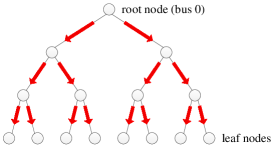
Figure 1: Radial topology of $\mathbb{G}$.

We orient the graph, without loss of generality, so that each line points away from bus 0. Denote a line in $\mathbb{E}$ by $(j,k)$ or $j\rightarrow k$ if it points from bus $j$ to bus $k$. Each bus $j$ (except bus 0) has a unique parent bus $i:=i_{j}$. Let $z_{jk}$ be the complex impedance of line $(j,k)\in\mathbb{E}$. Let $S_{jk}:=P_{jk}+\textbf{i}Q_{jk}$ denote the sending-end complex power from bus $j$ to bus $k$ where $P_{jk}$ and $Q_{jk}$ denote the real and reactive power flows. Let $l_{jk}$ denote the squared magnitude of the complex current from bus $j$ to bus $k$. Let $v_{j}$ denote the squared magnitude of the complex voltage phasor of bus $j$. We assume the voltage $v_{0}$ of bus 0 is fixed.

Each bus $j$ has a base load $s_{j}^{b}:=p^{b}_{j}+\textbf{i}q^{b}_{j}$ (excluding the battery charging loads from stations), where $p_{j}^{b}$ and $q_{j}^{b}$ denote the real and reactive power. Each bus $j$ may also have distributed generation $s_{j}^{g}:=p_{j}^{g}+\textbf{i}q_{j}^{g}$. Let $s_{j}$ denote the net complex power injection given by

$$s_{j} \!\!\!\!:=\!\!\!\! \left\{\begin{array}[]{ll}\!\!\!\!s^{g}_{j}-s^{b}_{j}-s^{e}_{j}&\text{ if $j$ supplies a station}\\ \!\!\!\!s^{g}_{j}-s^{b}_{j}&\text{ otherwise}\end{array}\right.$$

where $s^{e}_{j}$ denotes the total charging load at bus $j$. We assume the base loads $s_{j}^{b}$ are given and the generations $s_{j}^{g}$ and charging loads $s^{e}_{j}$ are variables.

We use the DistFlow equations proposed by Baran and Wu in [27] to model the power flows on the network:

$$\sum\limits_{k:(j,k)\in\mathbb{E}}{S_{jk}} =S_{ij}-z_{ij}l_{ij}+s_{j},\quad j\in\mathbb{N}$$ (2a)

$$v_{j}-v_{k} =2\mathrm{Re}(z_{jk}^{H}S_{jk})-|z_{jk}|^{2}l_{jk},\quad j\rightarrow k\in\mathbb{E}$$ (2b)

$$v_{j}l_{jk} =|S_{jk}|^{2},\quad j\rightarrow k\in\mathbb{E}$$ (2c)

where $v_{j}=:|V_{j}|^{2}$ and $l_{jk}:=|I_{jk}|^{2}$. The equations (2a) impose power balance at each bus, (2b) model the Ohm’s law, and (2c) define branch power flows. Note that $S_{i0}:=0$ and $I_{i0}:=0$ if $j=0$ is the substation bus. When bus $j$ is a leaf node of $\mathbb{G}$, all $S_{jk}=0$ in (2a). The quantity $z_{ij}|I_{ij}|^{2}$ is the loss on line $(i,j)$, and hence $S_{ij}-z_{ij}|I_{ij}|^{2}$ is the receiving-end complex power at bus $j$ from $i$.

The complex notation of the DistFlow equations (2) is only a shorthand for a set of real equations in the real vector variables $(s,v,l,S):=(p,q,v,l,P,Q):=(p_{j},q_{j},v_{j},l_{jk},P_{jk},Q_{jk},\,j,k\in\mathbb{N},\,(j,k)\in\mathbb{E})$. The equations (2a)–(2b) are linear in these variables but (2c) are quadratic, one of the two sources of nonconvexity in our joint battery swapping scheduling and OPF problem formulated below.

The operation of the distribution network must meet certain specifications. The squared voltage magnitudes must satisfy

$$\underline{v}_{j}\leq v_{j}\leq\overline{v}_{j},\quad j\in\mathbb{N}$$ (3a)

where $$\underline{v}_{j} \overline{v}_{j} j$$ and are given lower and upper bounds on the squared voltage magnitude at bus . The distributed real and reactive generations must satisfy

$$\underline{p}^{g}_{j}\leq p^{g}_{j}\leq\overline{p}^{g}_{j},\quad j\in\mathbb{N}$$ (3b)

$$\underline{q}^{g}_{j}\leq q^{g}_{j}\leq\overline{q}^{g}_{j},\quad j\in\mathbb{N}$$ (3c)

where $$\underline{p}^{g}_{j} \overline{p}^{g}_{j} \underline{q}^{g}_{j} \overline{q}^{g}_{j} j (j,k)$$, , , and are given lower and upper bounds on the real and reactive power generation at bus respectively. The power flows on line must satisfy

$$|S_{jk}|\leq\overline{S}_{jk},\quad j\rightarrow k\in\mathbb{E}$$ (3d)

where $\overline{S}_{jk}$ denotes the capacity of line $(j,k)$.

The model is quite general. For example, if a quantity is known and fixed, then we set both its upper and lower bounds to the given quantity, e.g., for the voltage of the substation bus, $\overline{v}_{0}=\underline{v}_{0}$. If there is no distributed generation at bus $j$ then $\overline{p}^{g}_{j}=\underline{p}^{g}_{j}=\overline{q}^{g}_{j}=\underline{q}^{g}_{j}=0$.

II-B Battery swapping scheduling

Let $\mathbb{N}_{w}:=\{1,2,\dots,N_{w}\}\subseteq\mathbb{N}$ denote the set of buses that supply electricity to stations. Their locations are fixed and known. There is a station connected to each bus $j\in\mathbb{N}_{w}$ and we use $j$ to index both the bus and the station. The batteries at station $j$ are either charging at a constant rate $r$ or already fully-charged and ready for swapping. Denote the total number of batteries and fully-charged batteries at the beginning of the current control interval by $M_{j}$ and $m_{j}$ respectively.

Let $\mathbb{A}:=\{1,2,\dots,A\}$ denote the set of EVs in the geographic area served by the distribution network that require battery swapping in the current interval. Let their states of charge be $(c_{a},{a\in\mathbb{A}})$. Let $u_{aj},~{}a\in\mathbb{A},~{}j\in\mathbb{N}_{w},$ represent the assignment:

$$u_{aj} = \left\{\begin{split}&1,\quad\mathrm{if~{}EV}~{}a~{}\mathrm{is~{}assigned~{}to~{}station}~{}j\\ &0,\quad\mathrm{otherwise}\end{split}\right.$$

and let ${u}:=(u_{aj},\,{a\in\mathbb{A},j\in\mathbb{N}_{w}}$) denote the vector of assignments.

Assumption 1. $A\leq\sum_{j\in\mathbb{N}_{w}}{m_{j}}$.

Under Assumption 1, there are enough fully-charged batteries in the system for all EVs in $\mathbb{A}$ in the current interval. This can be enforced when choosing the candidate set $\mathbb{A}$ of EVs for battery swapping, e.g., ranking EVs according to their states of charge and scheduling in an increasing order for at most $\sum_{j\in\mathbb{N}_{w}}{m_{j}}$ EVs.

The assignment $u$ satisfies the following conditions:

$$\sum\limits_{j\in\mathbb{N}_{w}}{u_{aj}} = 1,\quad a\in\mathbb{A}$$ (4a)

$$\sum\limits_{a\in\mathbb{A}}{u_{aj}} \leq m_{j},\quad j\in\mathbb{N}_{w}$$ (4b)

i.e., exactly one station is assigned to every EV and every assigned station has enough fully-charged batteries to serve EVs.

The system knows the current location of every EV $a$ and therefore can calculate the distance $d_{aj}$ from its current location to the assigned station $j$. If the EV is not currently carrying passengers and can go to swap its battery immediately, then $d_{aj}$ is the travel distance from its current location to station $j$, e.g., calculated from a routing application (such as Google map). If the EV must first complete its current passenger run before going to station $j$, then the distance $d_{aj}$ is the travel distance from its current location to the destination of its passengers and then to station $j$. The assigned station $j$ must be within each EV $a$’s driving range, i.e.,

$$u_{aj}d_{aj}\leq\gamma_{a}c_{a},\quad j\in\mathbb{N}_{w},a\in\mathbb{A}$$ (4c)

where $c_{a}$ is EV $a$’s current state of charge and $\gamma_{a}$ is its driving range per unit state of charge.

Since every EV produces a depleted battery that needs to be charged at rate $r$, we can express the net power injection $s_{j}=p_{j}+\textbf{i}q_{j}$ at bus $j$ in terms of assignment $u$ as:

$$p_{j} \!\!\!\!\!=\!\!\!\!\! \left\{\begin{split}&p_{j}^{g}-p_{j}^{b}-r\!\left(M_{j}-m_{j}+\sum_{a\in\mathbb{A}}{u_{aj}}\right)\!,&\!\!\!&j\in\mathbb{N}_{w}\\ &p_{j}^{g}-p_{j}^{b},&\!\!\!&j\in\mathbb{N}\setminus\mathbb{N}_{w}\end{split}\right.$$ (5a)

$$q_{j} \!\!\!\!=\!\!\! \ \ q_{j}^{g}-q_{j}^{b},\qquad j\in\mathbb{N}$$ (5b)

Let $f_{j}:\mathbb{R}\rightarrow\mathbb{R}$ models the generation cost at bus $j$, e.g., for a distributed gas generator. We assume all $f_{j}$ are strictly convex increasing functions [15, 17, 16]. We are interested in the following optimization problem:

$$\min\limits_{\bm{u},\bm{s},\bm{s}^{g},\atop\bm{v},\bm{l},\bm{S}} \sum\limits_{j\in\mathbb{N}}{f_{j}(p_{j}^{g})}+\alpha\sum\limits_{a\in\mathbb{A}}\sum\limits_{j\in\mathbb{N}_{w}}d_{aj}u_{aj}$$ (6)

$$\rm{s.t.} \eqref{eq:df}\eqref{eq:gridconstraints}\eqref{eq:uconstraints}\eqref{eq:inj},\ u_{aj}\in\{0,1\}$$

where $\sum\limits_{a\in\mathbb{A}}\sum\limits_{j\in\mathbb{N}_{w}}u_{aj}d_{aj}$ is the total travel distance of EVs and $\alpha>0$ is a weight that makes the generation cost and the travel distance comparable.

III Solution

The joint battery swapping scheduling and OPF problem (6) is generally difficult to solve because (2c) is nonconvex, as mentioned above, and $u$ is discrete. Our solution strategy has two steps.

1. SOCP relaxation. We first relax the nonconvex constraint (2c) into a second-order cone. Specifically, replace the DistFlow equations (2) by

$$\sum\limits_{k:(j,k)\in\mathbb{E}}{S_{jk}} =S_{ij}-z_{ij}l_{ij}+s_{j},\quad j\in\mathbb{N}$$ (7a)

$$v_{j}-v_{k} =2\mathrm{Re}(z_{jk}^{H}S_{jk})-|z_{jk}|^{2}l_{jk},\quad j\rightarrow k\in\mathbb{E}$$ (7b)

$$v_{j}l_{jk} \geq|S_{jk}|^{2},\quad j\rightarrow k\in\mathbb{E}$$ (7c)

Then the SOCP relaxation of the problem (6) is:

$$\min\limits_{\bm{u},\bm{s},\bm{s}^{g},\atop\bm{v},\bm{l},\bm{S}} \sum\limits_{j\in\mathbb{N}}{f_{j}(p_{j}^{g})}+\alpha\sum\limits_{a\in\mathbb{A}}\sum\limits_{j\in\mathbb{N}_{w}}d_{aj}u_{aj}$$ (8)

$$\rm{s.t.} \eqref{eq:df2}\eqref{eq:gridconstraints}\eqref{eq:uconstraints}\eqref{eq:inj},\ u_{aj}\in\{0,1\}$$

Fix any assignment $u\in\{0,1\}^{A}$. Then the problem (8) is a convex problem. It is a relaxation of the problem (6), given $u$, in the sense that the optimal objective value of the relaxation (8) lower bounds that of the original problem (6). If an optimal solution to the relaxation (8) attains equality in (7c) then the solution is also feasible, and therefore optimal, for the original problem (6). In this case, we say that the SOCP relaxation is exact. Sufficient conditions are known that guarantee the exactness of the SOCP relaxation; see [5, 6] for a comprehensive tutorial and references therein. Even when these conditions are not satisfied, SOCP relaxation for practical radial networks is often exact, as confirmed also by our simulations in Section IV.

Hence we will solve (8) instead of (6).

2. Generalized Benders decomposition. To deal with the discrete variables in (8), we apply generalized Benders decomposition. Benders decomposition was first proposed in [28] for problems where, when a subset of the variables are fixed, the remaining subproblem is a linear program. It is extended in [29] to the broader class of problems where the remaining subproblem is a convex program. We now apply it to solving (8).

Denote the continuous variables by $x:=(s,{s}^{g},{v},{l},{S})$ and the discrete variables by $u$. Denote the objective function by

$$F(x,u) := \sum\limits_{j\in\mathbb{N}}{f_{j}(p_{j}^{g})}+\alpha\sum\limits_{a\in\mathbb{A}}\sum\limits_{j\in\mathbb{N}_{w}}d_{aj}u_{aj}$$

Given any $u$, $F(x,u)$ is convex in $x$ since $f_{j}$’s are assumed to be strictly convex. Denote the constraint set for $x$ by

$$\mathbb{X} := \{x\in\mathbb{R}^{(5|\mathbb{N}|+3|\mathbb{E}|)}\,:\,x\text{ satisfies }\eqref{eq:gridconstraints}\eqref{eq:df2}\}$$

the constraint set for $u$ by

$$\mathbb{U} := \{u\in\{0,1\}^{AN_{w}}\,:\,u\text{ satisfies }\eqref{eq:uconstraints}\}$$

and the constraints (5) on $(x,u)$ by $G(x,u)=0$. Then the relaxation (8) takes the standard form for generalized Benders decomposition:

$$\min\limits_{x,u} F(x,u)$$ (9)

$$\rm{s.t.} G(x,u)=0,~{}x\in\mathbb{X},~{}u\in\mathbb{U}$$

where $F:\mathbb{R}^{(5|\mathbb{N}|+3|\mathbb{E}|)}\times\{0,1\}^{AN_{w}}\rightarrow\mathbb{R}$ is a scalar-valued function, and $G:\mathbb{R}^{(5|\mathbb{N}|+3|\mathbb{E}|)}\times\{0,1\}^{AN_{w}}\rightarrow\mathbb{R}^{2|\mathbb{N}|}$ is a vector-valued constraint function. Fixing any $u\in\mathbb{U}$, (9) is a convex subproblem in $x$. We now apply generalized Benders decomposition of [29] to (9).

Write (9) in the following equivalent form:

$$\min\limits_{u}\ \ W(u) \mathrm{s.t.}\qquad u\in\mathbb{U}\cap\mathbb{W}$$ (10a)

where

$$\begin{split}W(u):=\ &\min\limits_{x\in\mathbb{X}}\quad F(x,u)\\ &\ \mathrm{s.t.}\quad\ G(x,u)=0\end{split}$$ (10b)

and

$$\mathbb{W}:=\{u:G(x,u)=0\mathrm{~{}for~{}some}~{}x\in\mathbb{X}\}$$ (10c)

The problem (10b), called the slave problem, is convex and much easier to solve than (9). The set $\mathbb{W}$ consists of all $u$ for which (10b) is feasible and hence $\mathbb{U}\cap\mathbb{W}$ is the projection of the feasible region of (9) onto the $u$-space. The central idea of generalized Benders decomposition is to invoke the dual representations of $W(u)$ and $\mathbb{W}$ to derive the following equivalent problem to (10c) (see [29, Theorems 2.2 and 2.3]):

$$\min\limits_{u\in\mathbb{U}} \sup\limits_{\mu\in\mathbb{R}^{2|\mathbb{N}|}}\left\{\min\limits_{x\in\mathbb{X}}\left\{F(x,u)+\mu^{T}G(x,u)\right\}\right\}$$

$$\mathrm{s.t.} \min\limits_{x\in\mathbb{X}}\left\{\lambda^{T}G(x,u)\right\}=0,\quad\forall\lambda\in\mathbb{R}^{2|\mathbb{N}|}$$

Here $\lambda$ and $\mu$ are Lagrangian multiplier vectors for $\mathbb{W}$ and $W(u)$ respectively. This problem is equivalent to:

$$\min\limits_{u\in\mathbb{U},u_{0}} u_{0}$$ (11)

$$\mathrm{s.t.} u_{0}\geq\min\limits_{x\in\mathbb{X}}\left\{F(x,u)+\mu^{T}G(x,u)\right\},\ \ \forall\mu\in\mathbb{R}^{2|\mathbb{N}|}$$

$$\min\limits_{x\in\mathbb{X}}\left\{\lambda^{T}G(x,u)\right\}=0,\quad\forall\lambda\in\mathbb{R}^{2|\mathbb{N}|}$$

In summary, the series of manipulations has transformed the relaxation (8) into the master problem (11).

Since (11) has uncountably many constraints with all possible $\lambda$’s and $\mu$’s, it is neither practical nor necessary to enumerate all constraints in solving (11). Generalized Benders decomposition starts by solving a relaxed version of (11) that ignores all but a few constraints. If a solution of the relaxed version of (11) satisfies all the ignored constraints, then it is an optimal solution of (11) and the algorithm terminates. Otherwise, the solution process of the relaxed version of (11) will identify one $\mu$ or $\lambda$ for which the constraints are violated. These constraints are then added to the relaxed version of (11), and the cycle repeats.

Specifically the Benders decomposition algorithm for (8) (or equivalently (9)) is as follows.

• Step 1. Pick any $\bar{u}\in\mathbb{U}\cap\mathbb{W}$. Solve (10b) with $u=\bar{u}$ to obtain an optimal Lagrangian multiplier vector $\bar{\mu}$. Let $n_{\mu}=1$, $n_{\lambda}=0$, $\mu^{1}=\bar{\mu}$, and $UBD=W(\bar{u})$, where $n_{\mu}$, $n_{\lambda}$ are counters for the two types of constraints in (11), and $UBD$ denotes an upper bound on the optimal value of (9).

• Step 2. Solve the current relaxed master problem:

  $$\min\limits_{u\in\mathbb{U},u_{0}} u_{0}$$ (12)

  $$\mathrm{s.t.} u_{0}\geq\min\limits_{x\in\mathbb{X}}\left\{F(x,u)+\left({\mu^{i}}\right)^{T}G(x,u)\right\},$$

  $$\qquad\qquad\qquad\qquad\qquad\ \ i=1,\dots,n_{\mu}$$

  $$\min\limits_{x\in\mathbb{X}}\left\{\left({\lambda^{i}}\right)^{T}G(x,u)\right\}=0,$$

  $$\qquad\qquad\qquad\qquad\qquad\ \ i=1,\dots,n_{\lambda}$$

  Let $(\hat{u},\hat{u}_{0})$ be the optimal solution to (12). Clearly $\hat{u}_{0}$ is a lower bound on the optimal value of (9) since the constraints in (11) are relaxed to a smaller set of constraints in (12). Terminate the algorithm if $UBD-\hat{u}_{0}\leq\epsilon$, where $\epsilon>0$ is a sufficiently small threshold.

• Step 3. Solve the dual problem of (10b) with $u=\hat{u}$. The solution falls into the following two cases.

  1. Step 3a. The dual problem of (10b) has a finite solution $\hat{\mu}$. $W(\hat{u})$ is finite. Let $UBD=\min\{UBD,W(\hat{u})\}$. Terminate the algorithm if $UBD-\hat{u}_{0}\leq\epsilon$. Otherwise, increase $n_{\mu}$ by 1 and let $\mu^{n_{\mu}}=\hat{\mu}$. Return to Step 2.

  2. Step 3b. The dual problem of (10b) has an unbounded solution. Then (10b) is infeasible. Determine $\hat{\lambda}$ through a feasibility check problem and its dual [30]. Increase $n_{\lambda}$ by 1 and let $\lambda^{n_{\lambda}}=\hat{\lambda}$. Return to Step 2.

We make three remarks. First, the slave problem (10b) is convex and hence can generally be solved efficiently. The relaxed problem (12) involves discrete variables and are generally nonconvex, but it is much simpler than the original problem (9). Second, for our problem, (12) turns out to be a binary linear program because both $F$ and $G$ are separable functions in $(x,u)$ of the form:

$$F(x,u) =: f_{1}(x)+f_{2}(u)$$

$$G(x,u) =: g_{1}(x)+g_{2}(u)$$

where $f_{2}$ and $g_{2}$ are both linear in $u$. Indeed the constraints in (12) are

$$u_{0}-f_{2}(u)-\left({\mu^{i}}\right)^{T}g_{2}(u) \geq \min\limits_{x\in\mathbb{X}}\left\{f_{1}(x)+\left({\mu^{i}}\right)^{T}g_{1}(x)\right\}$$

$$\qquad\qquad\qquad i=1,\dots,n_{\mu}$$

$$\left({\lambda^{i}}\right)^{T}g_{2}(u) = -\min\limits_{x\in\mathbb{X}}\left({\lambda^{i}}\right)^{T}g_{1}(x)$$

$$\qquad\qquad\qquad i=1,\dots,n_{\lambda}$$

where the left-hand side is linear in the variable $u$ and the right-hand side is independent of $u$. Hence, in each iteration, the algorithm solves a binary linear program (12) and a convex program (10b). Finally, every time Step 2 is entered, one or two additional constraints are added to the binary linear program (12). This generally makes (12) harder to compute but also a better approximation of (11). It is proved in [29, Theorem 2.4] that the algorithm will terminate in finite steps since $\mathbb{U}$ is discrete and finite.

IV Numerical results

In this section, we evaluate the proposed algorithm through numerical simulations using a 56-bus distribution feeder of Southern California Edison (SCE) with a radial structure. More details about the feeder can be found in [31, Figure 2, TABLE I]. We add 4 distributed generators and 4 stations at different buses. The setup of the distributed generators is given in Table II(a). The 4 stations are assumed to be uniformly located in a 4km$\times$4km square area supplied by the distribution feeder, as shown in Table II(b). Suppose in a certain control interval, there are $A$ number of EVs that request battery swapping. Their current locations are randomized uniformly within the square area while their destinations are ignored. We use the Euclidean distance for $d_{aj}$. For convenience, it is assumed that $M_{j}=m_{j},~{}m_{j}=A,~{}j\in\mathbb{N}_{w}$, which means in each station batteries are all fully-charged and sufficient to serve all EVs. We assume all EVs have sufficient battery energy to reach any of the 4 stations, which means (4c) is readily satisfied. The extension to the general case where each EV has a limited driving range and can only reach some of the stations is straightforward. The constant charging rate is $r=0.01$MW [32] at all stations. To make the two components of the objective comparable, we set the weight $\alpha$ to be 0.02$/km first [33], and will then allow it to take different values to reveal its impact. Note that due to the randomness of EVs’ initialized locations, we conduct 10 simulation runs for each case setup. All numerical tests are run on a laptop with Intel Core i7-3632QM CPU@2.20GHz, 8GB RAM, and 64-bit Windows 10 OS.

TABLE I: Setup

Bus	$\overline{p}_{j}^{g}$	$\underline{p}_{j}^{g}$	$\overline{q}_{j}^{g}$	$\underline{q}_{j}^{g}$	Cost function
1	4	0	2	-2	$0.3{p^{g}}^{2}+30p^{g}$
4	2.5	0	1.5	-1.5	$0.1{p^{g}}^{2}+20p^{g}$
26	2.5	0	1.5	-1.5	$0.1{p^{g}}^{2}+20p^{g}$
34	2.5	0	1.5	-1.5	$0.1{p^{g}}^{2}+20p^{g}$

(a) Distributed generator

Bus	Location	$M_{j}$	$m_{j}$
5	(1,1)	$m_{j}$	$A$
16	(3,1)	$m_{j}$	$A$
31	(1,3)	$m_{j}$	$A$
43	(3,3)	$m_{j}$	$A$

(b) Station

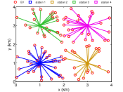
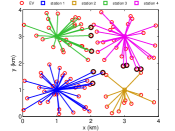
Figure 2: #EVs=100 (a) Nearest-station policy. (b) Optimal assignment.

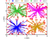
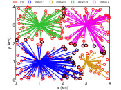
Figure 3: #EVs=300 (a) Nearest-station policy. (b) Optimal assignment.

Nearest-station policy. Without optimization, the default policy is that all EVs head for their nearest stations to swap batteries. This is shown in Fig. 2 and Fig. 3 for two specific cases with 100 and 300 EVs, respectively. In practice this myopic policy can lead to battery shortage at a station if many EVs cluster around that station due to correlation in traffic patterns. Moreover it can cause voltage instability: the voltage magnitudes of some buses drop below the threshold 0.95 p.u. in the 300-EV case, as shown in Table II.

TABLE II: Partial Bus data under nearest-station policy (300 EVs)

Bus	$|V_{j}|$ (p.u.)	$p_{j}^{g}$	$q_{j}^{g}$	$r\sum\limits_{a\in\mathbb{A}}{u_{aj}}$
1	1.050	0.571	0.000	/
4	1.047	2.500	0.663	/
5	1.031	/	/	0.660
16	0.941	/	/	0.700
18	0.948	/	/	/
19	0.944	/	/	/
26	1.050	2.500	0.410	/
31	1.020	/	/	0.830
34	1.044	2.500	1.500	/
43	1.015	/	/	0.810

Optimal assignment. Fig. 2 and Fig. 3 show the optimal assignments computed using the proposed algorithm for the above two cases, respectively. The nearest stations are not assigned to some of the EVs (marked black in the figures) when grid operational constraints such as voltage stability are taken into account. The numbers of such EVs is higher in the 300-EV case than that in the 100-EV case. The tradeoff between EVs’ total travel distance and the total generation cost is optimized. For comparison with Table II, the corresponding partial OPF results of the 300-EV case are listed in Table III. As we can see from Table III, the outputs (2.500 MW) of the distributed generators at buses 4, 26 and 34 have reached their full capacity (2.5 MW) while the injection (0.520 MW) at bus 1 (root bus) is far from its capacity (4 MW). This is consistent with our intuition that distributed generators that are closer to users and potentially cheaper than power from the transmission grid are favored in OPF. Under the optimal assignment, the deviations of voltages from their nominal value are all less than the 5%.

TABLE III: Partial Bus data under optimal assignment (300 EVs)

Bus	$|V_{j}|$ (p.u.)	$p_{j}^{g}$	$q_{j}^{g}$	$r\sum\limits_{a\in\mathbb{A}}{u_{aj}}$
1	1.050	0.520	0.000	/
4	1.048	2.500	0.590	/
5	1.025	/	/	0.990
15	0.981	/	/	/
16	0.974	/	/	0.300
17	0.980	/	/	/
18	0.973	/	/	/
19	0.969	/	/	/
26	1.050	2.500	0.439	/
31	1.019	/	/	0.840
34	1.044	2.500	1.500	/
43	1.013	/	/	0.870

Optimality of generalized Benders decomposition. The upper and lower bounds on the optimal objective values for the above two cases are plotted in Fig. 4 and Fig. 4, respectively, as the algorithm iterates between the master and slave problems. Basically, more iterations are required for larger-scale cases since it usually takes more iterations to attain an initial feasible solution. However, once we have a feasible solution, the gap between the upper and lower bounds starts to shrink rapidly and the convergence to optimality is achieved within a few iterations.

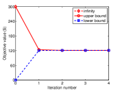
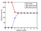
Figure 4: Convergence of generalized Benders decomposition (a) #EVs=100. (b) #EVs=300.

Exactness of SOCP relaxation. We check whether the solution computed by generalized Benders decomposition attains equality in (7c), i.e., whether the solution satisfies power flow equations and is implementable. Our final result confirms the exactness of the SOCP relaxation for the above two cases, and the relaxation is exact for most other cases we have tested on. Due to space limit, only some partial data of the 300-EV case are shown in Table IV.

In summary, SOCP relaxation and generalized Benders decomposition have solved our joint battery swapping scheduling and OPF problem (6) exactly.

TABLE IV: Exactness of SOCP relaxation (partial results for 300 EVs)

Bus		$v_{j}l_{jk}$	$|S_{jk}|^{2}$	Residual
From	To
1	2	0.271	0.271	0.000
2	3	0.006	0.006	0.000
2	4	0.202	0.202	0.000
4	5	1.369	1.369	0.000
4	6	0.005	0.005	0.000
4	7	1.952	1.952	0.000
7	8	1.691	1.691	0.000
8	9	0.009	0.009	0.000
8	10	1.269	1.269	0.000
10	11	1.092	1.092	0.000

Computational effort. To demonstrate the potential of the proposed algorithm for practical application, we check its required computational effort by counting its computation time for different number of EVs, since the number of discrete variables in the optimization problem is the computational bottleneck. We use Gurobi to solve the master problem (integer programming) and SDPT3 to solve the slave problem (convex programming) on the MATLAB R2012b platform. Fig. 5 shows the average computation time required by the proposed algorithm to find a global optimum for different numbers of EVs, which validates its computational efficiency.

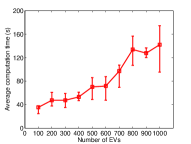
Figure 5: Average computation time as a function of #EVs.

Benefit. Fig. 6 displays the average relative reduction in the objective value with different $\alpha$’s using our algorithm, compared with the nearest-station policy. Scheduling flexibility is enhanced with more EVs, thus improving the savings. Clearly the smaller the weight $\alpha$ on EVs’ travel distance, the more benefit the proposed algorithm provides over the nearest-station policy. However, Fig.  6 also suggests that the improvement is small, i.e., the nearest-station policy is good enough if it is implementable.

The nearest-station policy is sometimes infeasible when there are more EVs nearest to a station than the number of fully-charged batteries at that station or when some operational constraints of the distribution network are violated. In our case study, infeasibility is mainly due to some voltages dropping below their lower limits. Define a metric voltage drop violation as $\mathrm{VDV}:=\sum_{j\in\mathbb{N}}\max\{\sqrt{\underline{v}_{j}}-|V_{j}|,0\}$ to quantify the degree of voltage violation. Fig. 7 shows the average VDV for the number of EVs ranging from 240 to 400 under the nearest-station policy. The voltage violation becomes more severe when the number of EVs increases.

It is also interesting to look at cases where there are more EVs nearest to a station than fully-charged batteries that station can provide, which, as far as we know, are common in practice. We reset $M_{1}=m_{1}=M_{2}=m_{2}=\frac{1}{2}A$ and $M_{3}=m_{3}=M_{4}=m_{4}=\frac{1}{8}A$ to simulate these situations. Hence the total number of fully-charged batteries in the system is $\frac{5}{4}A$. Fig. 8 shows, for each station, the average ratio of the number of EVs that go to the station for battery swapping to the number of fully-charged batteries at the station, under both the nearest-station policy and an optimal assignment. Under the optimal assignment, 99.40% of station 1’s batteries, 50.60% of station 2’s batteries, and all the batteries at stations 3, 4 are used, thus they have collectively served all $A$ EVs. Under the nearest-station policy, however, only 51.55% and 48.89% of stations 1 and 2’s batteries respectively (i.e., a total of around $\frac{1}{2}A$ batteries) are used for swapping. At either of stations 3 and 4, the number of EVs is approximately double that of available fully-charged batteries (192.61% and 205.62%, respectively). Fig. 8 shows the average number of unserved EVs under the nearest-station policy as a function of the total number $A$ of EVs. On average, a total of $\frac{1}{4}A$ EVs cannot be served at their nearest stations, mainly due to congestion at stations 3 and 4, while available fully-charged batteries at stations 1 and 2 are not fully utilized.

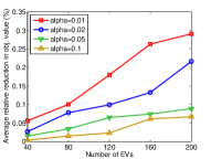
Figure 6: Average relative reduction in objective value.

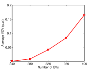
Figure 7: Average VDV under nearest-station policy.

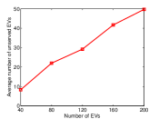
Figure 8: (a) Average ratio of the number of EVs to that of fully-charged batteries. (b) Average number of unserved EVs under nearest-station policy.

V Conclusion

We formulate an optimal scheduling problem for battery swapping that assigns to each EV a best station to swap its depleted battery based on its current location and state of charge. The schedule aims to minimize total travel distance and generation cost over both station assignments and power flow variables, subject to EV range constraints, grid operational constraints and AC power flow equations. We propose a centralized solution that relaxes the nonconvex constraint of OPF into a second-order cone and then applies generalized Benders decomposition to handle the binary nature of station assignments. Numerical case studies on the SCE 56-bus distribution feeder show the SOCP relaxation is mostly exact and generalized Benders decomposition computes an optimal solution efficiently.

References

- [1] C2ES, “Climate TechBook,” Center for Climate and Energy Solutions, US: www.c2es.org/energy/use/transportation, 2016.
- [2] EIA, “Monthly energy review,” Energy Information Administration, US Department of Energy: www.eia.gov/totalenergy/data/monthly/, 2015.
- [3] R.-C. Leou, C.-L. Su, and C.-N. Lu, “Stochastic analyses of electric vehicle charging impacts on distribution network,” IEEE Trans. on Power Systems, vol. 29, no. 3, pp. 1055–1063, 2014.
- [4] T. Shang, Y. Chen, and Y. Shi, “Orchestrating ecosystem co-opetition: Case studies on the business models of the EV demonstration programme in China,” Electric Vehicle Business Models, pp. 215–227, 2015.
- [5] S. H. Low, “Convex relaxation of optimal power flow, I: formulations and relaxations,” IEEE Trans. on Control of Network Systems, vol. 1, no. 1, pp. 15–27, 2014.
- [6] S. H. Low, “Convex relaxation of optimal power flow, II: exactness,” IEEE Trans. on Control of Network Systems, vol. 1, no. 2, pp. 177–189, 2014.
- [7] Z. Ma, D. Callaway, and I. Hiskens, “Decentralized charging control of large populations of plug-in electric vehicles,” IEEE Trans. on Control Systems Technology, vol. 21, no. 1, pp. 67–78, 2013.
- [8] L. Gan, U. Topcu, and S. H. Low, “Optimal decentralized protocol for electric vehicle charging,” IEEE Trans. on Power Systems, vol. 28, no. 2, pp. 940–951, 2013.
- [9] P. Papadopoulos, N. Jenkins, L. M. Cipcigan, I. Grau, and E. Zabala, “Coordination of the charging of electric vehicles using a multi-agent system,” IEEE Trans. on Smart Grid, vol. 4, no. 4, pp. 1802–1809, 2013.
- [10] S. Han, S. Han, and K. Sezaki, “Estimation of achievable power capacity from plug-in electric vehicles for V2G frequency regulation: Case studies for market participation,” IEEE Trans. on Smart Grid, vol. 2, no. 4, pp. 632–641, 2011.
- [11] A. O’Connell, D. Flynn, and A. Keane, “Rolling multi-period optimization to control electric vehicle charging in distribution networks,” IEEE Trans. on Power Systems, vol. 29, no. 1, pp. 340–348, 2014.
- [12] S. Chen and L. Tong, “iEMS for large scale charging of electric vehicles: Architecture and optimal online scheduling,” in Proc. of IEEE International Conference on Smart Grid Communications (SmartGridComm), pp. 629–634, 2012.
- [13] R. Li, Q. Wu, and S. S. Oren, “Distribution locational marginal pricing for optimal electric vehicle charging management,” IEEE Trans. on Power Systems, vol. 29, no. 1, pp. 203–211, 2014.
- [14] Z. Yu, S. Li, and L. Tong, “On market dynamics of electric vehicle diffusion,” in Proc. of the 52nd Annual Allerton Conferene on Communication, Control, and Computing, pp. 1051–1057, 2014.
- [15] S. Sojoudi and S. H. Low, “Optimal charging of plug-in hybrid electric vehicles in smart grids,” in Proc. of IEEE Power & Energy Society General Meeting, pp. 1–6, 2011.
- [16] L. Zhang, V. Kekatos, and G. B. Giannakis, “Scalable network-constrained electric vehicle charging in multiphase distribution grids,” arXiv preprint arXiv:1510.00403, 2015.
- [17] N. Chen, C. W. Tan, and T. Q. Quek, “Electric vehicle charging in smart grid: Optimality and valley-filling algorithms,” IEEE Journal of Selected Topics in Signal Processing, vol. 8, no. 6, pp. 1073–1083, 2014.
- [18] J. de Hoog, T. Alpcan, M. Brazil, D. A. Thomas, and I. Mareels, “Optimal charging of electric vehicles taking distribution network constraints into account,” IEEE Trans. on Power Systems, vol. 30, no. 1, pp. 365–375, 2015.
- [19] J. Franco, M. Rider, and R. Romero, “A mixed-integer linear programming model for the electric vehicle charging coordination problem in unbalanced electrical distribution systems,” IEEE Trans. on Smart Grid, vol. 6, no. 5, pp. 2200–2210, 2015.
- [20] X. Tan, B. Sun, and D. H. Tsang, “Queueing network models for electric vehicle charging station with battery swapping,” in Proc. of IEEE International Conference on Smart Grid Communications (SmartGridComm), pp. 1–6, 2014.
- [21] S. Yang, J. Yao, T. Kang, and X. Zhu, “Dynamic operation model of the battery swapping station for EV (electric vehicle) in electricity market,” Energy, vol. 65, pp. 544–549, 2014.
- [22] P. You, Z. Yang, Y. Zhang, S. H. Low, and Y. Sun, “Optimal charging schedule for a battery switching station serving electric buses,” IEEE Trans. on Power Systems, vol. 31, no. 5, pp. 3473–3483, 2016.
- [23] M. R. Sarker, H. Pandžić, and M. A. Ortega-Vazquez, “Optimal operation and services scheduling for an electric vehicle battery swapping station,” IEEE Trans. on Power Systems, vol. 30, no. 2, pp. 901–910, 2015.
- [24] Y. Zheng, Z. Y. Dong, Y. Xu, K. Meng, J. H. Zhao, and J. Qiu, “Electric vehicle battery charging/swap stations in distribution systems: comparison study and optimal planning,” IEEE Trans. on Power Systems, vol. 29, no. 1, pp. 221–229, 2014.
- [25] X. Zhang and R. Rao, “A benefit analysis of electric vehicle battery swapping and leasing modes in china,” Emerging Markets Finance and Trade, vol. 52, no. 6, pp. 1414–1426, 2016.
- [26] Q. Wang, K. Qin, and D. Chen, “Power supply radius optimization for substations with large capacity transformers.” http://www.cqvip.com/read/read.aspx?id=83887068504849524852484852.
- [27] M. E. Baran and F. F. Wu, “Optimal capacitor placement on radial distribution systems,” IEEE Trans. on Power Delivery, vol. 4, no. 1, pp. 725–734, 1989.
- [28] J. F. Benders, “Partitioning procedures for solving mixed-variables programming problems,” Numerische mathematik, vol. 4, no. 1, pp. 238–252, 1962.
- [29] A. M. Geoffrion, “Generalized benders decomposition,” Journal of optimization theory and applications, vol. 10, no. 4, pp. 237–260, 1972.
- [30] P. You, Z. Yang, M. Y. Chow, and Y. Sun, “Optimal cooperative charging strategy for a smart charging station of electric vehicles,” IEEE Trans. on Power Systems, vol. 31, no. 4, pp. 2946–2956, 2016.
- [31] M. Farivar, R. Neal, C. Clarke, and S. Low, “Optimal inverter var control in distribution systems with high PV penetration,” in Proc. of IEEE Power & Energy Society General Meeting, pp. 1–7, 2012.
- [32] M. Yilmaz and P. T. Krein, “Review of battery charger topologies, charging power levels, and infrastructure for plug-in electric and hybrid vehicles,” IEEE Trans. on Power Electronics, vol. 28, no. 5, pp. 2151–2169, 2013.
- [33] EIA, “Annual energy review,” Energy Information Administration, US Department of Energy: www.eia.doe.gov/emeu/aer, 2011.