Multi-Modal Mean-Fields via Cardinality-Based Clamping

Abstract

Mean Field inference is central to statistical physics. It has attracted much interest in the Computer Vision community to efficiently solve problems expressible in terms of large Conditional Random Fields. However, since it models the posterior probability distribution as a product of marginal probabilities, it may fail to properly account for important dependencies between variables.

We therefore replace the fully factorized distribution of Mean Field by a weighted mixture of such distributions, that similarly minimizes the KL-Divergence to the true posterior. By introducing two new ideas, namely, conditioning on groups of variables instead of single ones and using a parameter of the conditional random field potentials, that we identify to the temperature in the sense of statistical physics to select such groups, we can perform this minimization efficiently. Our extension of the clamping method proposed in previous works allows us to both produce a more descriptive approximation of the true posterior and, inspired by the diverse MAP paradigms, fit a mixture of Mean Field approximations. We demonstrate that this positively impacts real-world algorithms that initially relied on mean fields.

1 Introduction

Mean Field (MF) is a modeling technique that has been central to statistical physics for a century. Its ability to handle stochastic models involving millions of variables and dense graphs has attracted much attention in our community. It is routinely used for tasks as diverse as detection [13, 2], segmentation [31, 23, 9, 41], denoising [10, 27, 25], depth from stereo [14, 23] and pose-estimation [34].

MF approximates a “true” probability distribution by a fully-factorized one that is easy to encode and manipulate [22]. The true distribution is usually defined in practice through a Conditional Random Field (CRF), and may not be representable explicitly, as it involves complex inter-dependencies between variables. In such a case the MF approximation is an extremely useful tool.

While this drastic approximation often conveys the information of interest, the true distribution may concentrate on configurations that are very different, equally likely, and that cannot be jointly encoded by a product law. Section 3 depicts such a case where groups of variables are correlated and may take one among many values with equal probability. In this situation, MF will simply pick one valid configuration, which we call a mode, and ignore the others. So-called structured Mean Field methods [32, 7] can help overcome this limitation. This can be effective but requires arbitrary choices in the design of a simplified sub-graph for each new problem, which can be impractical especially if the initial CRF is very densely connected.

Here we introduce a novel way to automatically add structure to the MF approximation and show how it can be used to return several potentially valid answers in ambiguous situations. Instead of relying on a single fully factorized probability distribution, we introduce a mixture of such distributions, which we will refer to as Multi-Modal Mean Field (MMMF).

We compute this MMMF by partitioning the state space into subsets in which a standard MF approximation suffices. This is similar in spirit to the approach of [37] but a key difference is that our clamping acts simultaneously on arbitrarily sized groups of variables, as opposed to one at a time. We will show that when dealing with large CRFs with strong correlations, this is essential. The key to the efficiency of MMMF is how we choose these groups. To this end, we introduce a temperature parameter that controls how much we smooth the original probability distribution before the MF approximation. By doing so for several temperatures, we spot groups of variables that may take different labels in different modes of the distribution. We then force the optimizer to explore alternative solutions by clamping them, that is, forcing them to take different values. Our temperature-based approach, unlike the one of [37], does not require a priori knowledge of the CRF structure and is therefore compatible with “black box” models.

In the remainder of the paper, we will describe both MF and MMMF in more details. We will then demonstrate that MMMF outperforms both MF and the clamping method of [37] on a range of tasks.

2 Background and Related Work

Conditional Random Fields (CRFs) are often used to represent correlations between variables [36]. Mean Field inference is a means to approximate them in a computationally efficient way. We briefly review both techniques below.

2.1 Conditional Random Fields

Let $\mathbf{X}=\left(X_{1},\ldots,X_{N}\right)$ represent hidden variables and $\mathbf{I}$ an image evidence. A CRF relates the ones to the others via a posterior probability distribution

$$\vspace{-0.2cm}P(\mathbf{X}\mid\mathbf{I}) =\exp\left(-\mathcal{E}(\mathbf{X}\mid\mathbf{I})-\log(Z(\mathbf{I}))\right)\;,\vspace{-0.1cm}$$ (1)

where $\mathcal{E}(\mathbf{X}\mid\mathbf{I})$ is an energy function that is the sum of terms known as potentials $\bm{\phi}_{c}(\cdot)$ defined on a set of graph cliques $c\in\mathcal{C}$, $\log(Z(\mathbf{I}))$ is the log-partition function that normalizes the distribution. From now on, we will omit the dependency with respect to $\mathbf{I}$.

2.2 Mean Field Inference

The set of all possible configurations of $\mathbf{X}$, that we denote by $\mathcal{X}$, is exponentially large, which makes the explicit computation of marginals, Maximum-A-Posteriori (MAP) or $Z$ intractable and a wide range of variational methods have been proposed to approximate $P(\mathbf{X})$ [19]. Among those, Mean Field (MF) inference is one of the most popular. It involves introducing a distribution $Q$ written as

$$\vspace{-0.2cm}Q(\mathbf{X}=(x_{1},\ldots,x_{N}))=\prod_{i=1}^{N}q_{i}(x_{i})\;,\vspace{-0.1cm}$$ (2)

where $q_{i}(\,.\,)$ is a categorical discrete distribution defined for $x_{i}$ in a possible labels space $\mathcal{L}$. The $q_{i}$ are estimated by minimizing the KL-divergence

$$\text{KL}(Q||P)=\sum_{\mathbf{x}\in\mathcal{X}}Q(\mathbf{X}=\mathbf{x})\log\frac{Q(\mathbf{X}=\mathbf{x})}{P(\mathbf{X}=\mathbf{x})}\;.$$ (3)

Since $Q$ is fully factorized, the terms of the KL-divergence can be recombined as a sum of an expected energy, containing as many terms as there are potentials and a convex negative entropy containing one term per variable. Optimization can then be performed using a provably convergent gradient-descent scheme [3].

As will be shown in Section 3, this simplification sometimes comes at the cost of downplaying the dependencies between variables. The DivMBest method [29, 4] addresses this issue starting from the following observation: When looking for an assignment in a graphical model, the resulting MAP is not necessarily the best because the probabilistic model may not capture all that is known about the problem. Furthermore, optimizers can get stuck in local minima. The proposed solution is to sequentially find several local optima and force them to be different from each other by introducing diversity constraints in the objective function. It has recently been shown that it is provably more effective to solve for diverse MAPs jointly but under the same set of constraints [20]. However, none of these methods provide a generic and practical way to choose local constraints to be enforced over variable sub-groups. Furthermore, they only return a set of MAPs. By contrast, our approach yields a multi-modal approximation of the posterior distribution, which is a much richer description and which we will show to be useful.

Another approach to improving the MF approximation is to decompose it into a mixture of product laws by “clamping” some of the variables to fixed values, and finding for each set of values the best factorized distribution under the resulting deterministic conditioning. By summing the resulting approximations of the partition function, one can provably improve the approximation of the true partition function [37]. This procedure can then be repeated iteratively by clamping successive variables but is only practical for relatively small CRFs. At each iteration, the variable to be clamped is chosen on the basis of the graphical model weights, which requires intimate knowledge about its internals, which is not always available.

Our own approach is in the same spirit but can clamp multiple variables at a time without requiring any knowledge of the graph structure or weights.

Finally, DivMBest approaches do not provide a way to choose the best solution without looking at the ground-truth, except for the one of [39] that relies on training a new classifier for that purpose. By contrast, we will show that the multi modal Bayesian nature of our output induces a principled way to use temporal consistency to solve directly practical problems.

3 Motivation

To motivate our approach, we present here a toy example that illustrates a typical failure mode of the standard MF technique, which ours is designed to prevent. Fig. 1 depicts a CRF where each pixel represents a binary variable connected to its neighbors by attractive pairwise potentials.

For the sake of illustration, we split the grid into four zones as follows. The attractive terms are weak on left side but strong on the right. Similarly, in the top part, the unary terms favor value of $1$ while being completely random in the bottom part.

The unary potentials are depicted at the top left of Fig. 1 and the result of the standard MF approximation at the bottom in terms of the probability of the pixels being assigned the label $1$. In the bottom right corner of the grid, because the interaction potentials are strong, all pixels end up being assigned high probabilities of being 1 by MF, where they could just as well have all been assigned high probabilities to be zero. We explain below how our MMMF algorithm can produce two equally likely modes, one with all pixels being zero with high probability and the other with all pixel being one with high probability.

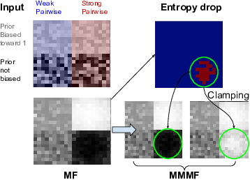
Figure 1: A typical failure mode of MF resolved by MMMF. Grey levels indicate marginal probabilities, under the prior (Input) and under the product laws (MF and MMMF).

4 Multi-Modal Mean Fields

Given a CRF defined with respect to a graphical model and the probability $P(\mathbf{X}=\mathbf{x})$ for all states in $\mathcal{X}$, the state space introduced in Section 2.1, the standard MF approximation only models a single mode of the $P$, as discussed in Section 2.2. We therefore propose to create a richer representation that accounts for potential multiple modes by replacing the fully factorized distribution of Eq. 2 by a weighted mixture of such distributions that better minimizes the KL-divergence to $P$.

The potential roadblock is the increased difficulty of the minimization problem. In this section, we present an overview of our approach to solving it, and discuss its key aspects in the following two.

Formally, let us assume that we have partitioned $\mathcal{X}$ into disjoint subsets $\mathcal{X}_{k}$ for $1\leq k\leq K$. We replace the original Mean Field (MF) approximation by one of the form

$$P(\mathbf{X}=\mathbf{x})\ \approx\ Q_{MM}(\mathbf{X}=\mathbf{x}) \!\!\!\!=\!\!\!\! \sum_{k}m_{k}Q_{k}(\mathbf{x})\;,$$ (4)

$$Q_{k}(\mathbf{x}) \!\!\!\!=\!\!\!\! \prod_{i}{q_{i}^{k}(x_{i})}\;,$$

where $Q_{k}$ is a MF approximation for the states $\mathbf{x}\in\mathcal{X}_{k}$ with individual probabilities $q_{i}^{k}$ that variable $i$ can take value $x_{i}$ in a set of labels $\mathcal{L}$, and $m_{k}$ is the probability that a state belongs to $\mathcal{X}_{k}$.

We can evaluate the $m_{k}$ and $q_{i}^{k}$ values by minimizing the KL-divergence between $Q_{MM}$ and $P$. The key to making this computation tractable is to guarantee that we can evaluate the $q_{i}^{k}$ parameters on each subset separately by performing a standard MF approximation for each. One way to achieve that is to constrain the support of the $Q_{k}$ distributions to be disjoint, that is,

$$\forall k\neq k^{\prime},Q_{k^{\prime}}\left(\mathcal{X}_{k}\right) = 0\;.$$ (5)

In other words, each MF approximation is specialized on a subset $\mathcal{X}_{k}$ of the state space and is computed to minimize the KL-Divergence there. In practice, we enrich our approximation by recursively splitting a set of states $\mathcal{X}_{k}$ among our partition $\mathcal{X}_{1},\dots,\mathcal{X}_{K}$ into two subsets $\mathcal{X}^{1}_{k}$ and $\mathcal{X}^{2}_{k}$ to obtain the new partition $\mathcal{X}_{1},\dots,\mathcal{X}_{k-1},\mathcal{X}^{1}_{k},\mathcal{X}^{2}_{k},\mathcal{X}_{k+1},\dots,\mathcal{X}_{K}$, which is then reindexed from $1$ to $K+1$. Initially, $\mathcal{X}_{k}$ represents the whole state space. Then we take it to be the newly created subset in a breadth-first order until a preset number of subsets has been reached. Each time, the algorithm proceeds through the following steps:

• It finds groups of variables likely to have different values in different modes of the distribution using an entropy-based criterion for the $q_{i}^{k}$.

• It partitions the set into two disjoint subsets according to a clause that sets a threshold on the number of variables in this group that take a specific label. $\mathcal{X}^{1}_{k}$ will contain the states among $\mathcal{X}_{k}$ that meet this clause and $\mathcal{X}^{2}_{k}$ the others.

• It performs an MF approximation within each subset independently to compute parameters $q_{i}^{k,1}$ and $q_{i}^{k,2}$ for each of them. This is done by a standard MF approximation, to which we add the disjointness constraint 5.

This yields a binary tree whose leaves are the $\mathcal{X}_{k}$ subsets forming the desired state-space partition. Given this partition, we can finally evaluate the $m_{k}$. In Section 5, we introduce our cardinality based criterion and show that it makes minimization of the KL-divergence possible. In Section 6, we show how our entropy-based criterion selects, at each iteration, the groups of variables on which the clauses depend.

5 Partitioning the State Space

In this section, we describe the cardinality-based criterion we use to recursively split state spaces and explain why it allows efficient optimization of the KL-divergence $\text{KL}(Q_{MM}\|P)$, where $Q_{MM}$ is the mixture of Eq. 4.

5.1 Cardinality Based Clamping

The state space partition $\mathcal{X}_{k\;,\;{1\leq k\leq K}}$ introduced above is at the heart of our approximation and its quality and tractability critically depend on how well chosen it is. In [37], each split is obtained by clamping to zero or one the value of a single binary variable. In other words, given a set of states $\mathcal{X}_{k}$ to be split, it is broken into subsets $\mathcal{X}_{k}^{1}=\{\mathbf{x}\in\mathcal{X}_{k}|x_{i}=0\}$ and $\mathcal{X}_{k}^{2}=\{\mathbf{x}\in\mathcal{X}_{k}|x_{i}=1\}$, where $i$ is the index of a specific variable. To compute a Mean Field approximation to $P$ on each of these subspaces, one only needs to perform a standard Mean Field approximation while constraining the $q_{i}$ probability assigned to the clamped variable to be either zero or one. However, this is limiting for the large and dense CRFs used in practice because clamping only one variable among many at a time may have very little influence overall. Pushing the solution towards a qualitatively different minimum that corresponds to a distinct mode may require simultaneously clamping many variables.

To remedy this, we retain the clamping idea but apply it to groups of variables instead of individual ones so as to find new modes of the posterior while keeping the estimation of the parameters $m_{k}$ and $q^{k}_{i}$ computationally tractable. More specifically, given a set of states $\mathcal{X}_{k}$ to be split, we will say that the split into $\mathcal{X}^{1}_{k}$ and $\mathcal{X}^{2}_{k}$ is cardinality-based if

$$\mathcal{X}^{1}_{k}=\{\mathbf{x}\in\mathcal{X}_{k}\text{ s.t. }\sum\limits_{u=1\dots L}\mathbbm{1}(\mathbf{x}_{i_{u}}=v_{u})\geq C\}\;,$$ (6)

$$\mathcal{X}^{2}_{k}=\{\mathbf{x}\in\mathcal{X}_{k}\text{ s.t. }\sum\limits_{u=1\dots L}\mathbbm{1}(\mathbf{x}_{i_{u}}=v_{u})<C\}\;,$$ (7)

where the $i_{1},\dots,i_{L}$ denote groups of variables that are chosen by the entropy-based criterion and $v_{1},\dots,v_{L}$ is a set of labels in $\mathcal{L}$. In other words, in one of the splits, more than $C$ of the variables have the assigned values and in the other less than $C$ do. For example, for semantic segmentation $\mathcal{X}^{1}_{k}$ would be the set of all segmentations in $\mathcal{X}_{k}$ for which at least $C$ pixels in a region take a given label, and $\mathcal{X}^{2}_{k}$ the set of all segmentations for which less than $C$ pixels do.

We will refer to this approach as cardinality clamping and will propose a practical way to select appropriate $i_{1},\dots,i_{L}$ and $v_{1},\dots,v_{L}$ for each split in Section 6.

5.2 Instantiating the Multi-Modal Approximation

The cardinality clamping scheme introduced above yields a state space partition $\mathcal{X}_{k\;,\;{1\leq k\leq K}}$. We now show that given such a partition, minimizing the KL-divergence $\text{KL}(Q_{MM}\|P)$ using the multi-modal approximation of Eq. 4 under the disjointness constraint, becomes tractable.

In practice, we relax the constraint 5 to near disjointness

$$\forall k\neq k^{\prime},Q_{k^{\prime}}\left(\mathcal{X}_{k}\right)\leq\epsilon\;,$$ (8)

where $\epsilon$ is a small constant. It makes the optimization problem better behaved and removes the need to tightly constrain any individual variable, while retaining the ability to compute the KL divergence up to $\mathcal{O}(\epsilon\log(\epsilon))$.

Let $\hat{m}$ and $\hat{q}$ stand for all the $m_{k}$ and $q_{i}^{k}$ parameters that appear in Eq. 4. We compute them as

$$\min\limits_{\hat{m},\hat{q}}\text{KL}(Q_{MM}\|P) = \min\limits_{\hat{m},\hat{q}}\sum\limits_{\mathbf{x}\in\mathcal{X}}\sum\limits_{k\leq K}m_{k}Q_{k}(\mathbf{x})\log\left(\dfrac{Q_{MM}(\mathbf{x})}{P(\mathbf{x})}\right)$$ (9)

$$\equiv \min\limits_{\hat{m}}\sum\limits_{k\leq K}m_{k}\log(m_{k})-\sum\limits_{k\leq K}m_{k}A_{k}\;,$$

$$\mbox{where \hskip 22.76228pt}A_{k} = \max\limits_{q^{k}_{i},{i=1\dots N}}\sum\limits_{\mathbf{x}\in\mathcal{X}}Q_{k}(\mathbf{x})\log\left(\dfrac{e^{-E(\mathbf{x})}}{Q_{k}(\mathbf{x})}\right)\;$$ (10)

where $A_{k}$ is maximized under the near-disjointness constraint of Eq. 16.

As proved formally in the supplementary material, the second equality of Eq. 9 is valid up to a constant and after neglecting a term of order $\mathcal{O}(\epsilon\log\epsilon)$ which appears under the near disjointness assumption of the supports. Given the $A_{k}$ terms of Eq. 10 and under the constraints that the mixture probabilities $\hat{m}$ sum to one, we must have

$$m_{k}=\dfrac{e^{A_{k}}}{\sum\limits_{k^{\prime}\leq K}e^{A_{k^{\prime}}}}\;,$$ (11)

and we now turn to the computation of these $A_{k}$ terms. We formulate it in terms of a constrained optimization problem as follows.

5.2.1 Handling Two Modes

Let us first consider the case where we generate only two modes modeled by $Q_{1}(\mathbf{x})=\prod q^{1}_{i}(x_{i})$ and $Q_{2}(\mathbf{x})=\prod q^{2}_{i}(x_{i})$ and we seek to estimate the $q^{1}_{i}$ probabilities. The $q^{2}_{i}$ probabilities are evaluated similarly.

Recall from Section 5.2 that the $q^{1}_{i}$ must be such that the $A_{1}$ term of Eq. 10 is maximized subject to the near disjointness constraint of Eq. 16, which becomes

$$Q_{1}\left(\sum\limits_{u=1\dots L}\mathbbm{1}(\mathbf{X}_{i_{u}}=v_{u})<C\right)\leq\epsilon\;,$$ (12)

under our cardinality-based clamping scheme defined by Eq. 7. Performing this maximization using a standard Lagrangian Dual procedure [8] requires evaluating the constraint and its derivatives. Despite the potentially exponentially large number of terms involved, we can do this in one of two ways. In both cases, the Lagrangian Dual procedure reduces to a series of unconstrained Mean Field minimizations with well known additional potentials.

1. When $C$ is close to $0$ or to $L$, the Lagrangian term can be treated as a specific form of pattern-based higher-order potentials, as in [35, 13, 21, 1].

2. When $C$ is both substantially greater than zero and smaller than $L$, we treat $\sum_{u=1\dots L}\mathbbm{1}(\mathbf{X}_{i_{u}}=v_{u})$ as a large sum of independent random variables under $Q_{1}$. We therefore use a Gaussian approximation to replace the cardinality constraint by a simpler linear one, and finally add unary potentials to the MF problem. Details are provided in the supplementary material.

We will encounter the first situation when tracking pedestrians and the second when performing semantic segmentation, as will be discussed in the results section.

5.2.2 Handling an Arbitrary Number of Nodes

Recall from Section 5 that, in the general case, there can be an arbitrary number of modes. They correspond to the leaves of a binary tree created by a succession of cardinality-based splits. Let us therefore consider mode $k$ for $1\leq k\leq K$. Let $B$ be the set of branching points on the path leading to it. The near disjointness 16, can be enforced with only $|B|$ constraints. For each $b\in B$, there is a list of variables $i^{b}_{1},\dots,i^{b}_{L^{b}}$, a list of values $v^{b}_{1},\dots,v^{b}_{L^{b}}$, a cardinality threshold $C^{b}$, and a sign for the inequality $\geq_{b}$ that define a constraint

$$Q_{k}\left(\sum\limits_{u=1\dots L^{b}}\mathbbm{1}(\mathbf{X}_{i^{b}_{u}}=v^{b}_{u})\geq_{b}C^{b}\right)\leq\epsilon$$ (13)

of the same form as that of Eq. 12. It ensures disjointness with all the modes in the subtree on the side of $b$ that mode $k$ does not belong to. Therefore, we can solve the constrained maximization problem of Eq. 10, as in Section 5.2.1, but with $|B|$ constraints instead of only one.

6 Selecting Variables to Clamp

We now present an approach to choosing the variables $i_{1},\dots,i_{L}$ and the values $v_{1},\dots,v_{L}$, which define the cardinality splits of Eqs. 6 and 7, that relies on phase transitions in the graphical model.

To this end, we first introduce a temperature parameter in our model that lets us smooth the probability distribution we want to approximate. This well known parameter for physicists [18] was used in a different context in vision by [28]. We study its influence on the corresponding MF approximation and how we can exploit the resulting behavior to select appropriate values for our variables.

6.1 Temperature and its Influence on Convexity

We take the temperature $T$ to be a number that we use to redefine the probability distribution of Eq. 1 as

$$\vspace{-1mm}P^{T}(\mathbf{x})=\dfrac{1}{Z^{T}}e^{-\small{\dfrac{1}{T}}\mathcal{E}(\mathbf{x})}\;,$$ (14)

where $Z^{T}$ is the partition function that normalizes $P^{T}$ so that its integral is one. For $T=1$, $P^{T}$ reduces to $P$. As $T$ goes to infinity, it always yields the same Maximum-A-Posteriori value but becomes increasingly smooth. When performing the MF approximation at high $T$, the first term of the KL-Divergence, the convex negative entropy, dominates and makes the problem convex. As $T$ decreases, the second term of the KL-Divergence, the expected energy, becomes dominant, the function stops being convex, and local minima can start to appear. In the supplementary material, we introduce a physics-inspired proof that, in the case of a dense Gaussian CRF [23], we can approximate and upper-bound, in closed-form, the critical temperature $T_{c}$ at which the KL divergence stops being convex. We validate experimentally this prediction, using directly the denseCRF code from [23]. This makes it easy to define a temperature range $[1,T_{max}]$ within which to look for $T_{c}$. For a generic CRF, no such computation may be possible and the range must be determined empirically.

6.2 Entropy-Based Splitting

We describe here our approach to splitting $\mathcal{X}$ into $\mathcal{X}_{1}$ and $\mathcal{X}_{2}$ at the root node of the tree. The subsequent splits are done in exactly the same way. The variables to be clamped are those whose value change from one local minimum to another so that we can force the exploration of both minima.

To find them, we start at $T_{max}$, a temperature high enough for the KL divergence to be convex and progressively reduce it. For each successive temperature, we perform the MF approximation starting with the estimate for the previous one to speed up the computation. When looking at the resulting set of approximations starting from the lowest temperature ones $T=1$, a telltale sign of increasing convexity is that the assignment of some variables that were very definite suddenly becomes uncertain. Intuitively, this happens when the CRF terms that bind variables is overcome by the entropy terms that encourage uncertainty. In physical terms, this can be viewed as a local phase-transition [18].

Let $T$ be a temperature greater than $1$ and let $Q^{T}$ and $Q^{1}$ be the corresponding Mean Field approximations, with their marginal probabilities $q^{T}_{i}$ and $q^{1}_{i}$ for each variable $i$. To detect such phase transitions, we compute

$$\delta_{i}(T)=\mathbbm{1}[\mathcal{H}(q^{T}_{i})>h_{high}]\mathbbm{1}[\mathcal{H}(q^{1}_{i})<h_{low}]\;,$$ (15)

for all $i$, where $\mathcal{H}$ denotes the individual entropy.

All variables and labels with positive $\delta_{i}$ become candidates for clamping. If there are none, we increase the temperature. If there are several, we can either pick one at random or use domain knowledge to pick the most suitable subset and values as will be discussed in the Results Section.

7 Results

We first use synthetic data to demonstrate that MMMF can approximate a multi-modal probability density function better than both standard MF and the recent approach of [37], which also relies on clamping to explore multiple modes. We then demonstrate that this translates to an actual performance gain for two real-world algorithms—one for people detection [13] and the other for segmentation [9, 40]—both relying on a traditional Mean Field approach. We will make all our code and test datasets publicly available.

The parameters that control MMMF are the number of modes we use, the cardinality threshold $C$ at each split, the $\epsilon$ value of Eq. 16, the entropy thresholds $h_{low}$ and $h_{high}$ of Eq. 15, and the temperature $T_{\max}$ introduced in Section 6. In all our experiments, we use $\epsilon=10^{-4}$, $h_{low}=0.3$, and $h_{high}=0.7$. As discussed in Section 6, when the CRF is a dense Gaussian CRF, we can approximate and upper bound the critical temperature $T_{c}$ in closed-form and we simply take $T_{\max}$ to be this upper bound to guarantee that $T_{\max}>T_{c}$. Otherwise, we choose $T_{\max}$ empirically on a small validation-set and fix it during testing.

7.1 Synthetic Data

To demonstrate that our approach minimizes the KL-Divergence better than both standard MF and the clamping one of [37], we use the same experimental protocol to generate conditional random fields with random weights as in [12, 38, 37]. Our task is then to find the MMMF approximation with lowest KL-Divergence for any given number of nodes. When that number is one, it reduces to MF. Note that the authors of [37] look for an approximation of the log-partition function, which is strictly the same as minimizing the KL-Divergence, as demonstrated in the supplementary material. Because it involves randomly chosen positive and negative weights, this problem effectively mimics difficult real-world ones with repulsive terms, uncontrolled loops, and strong correlations.

In Fig. 2, we plot the KL-Divergence as a function of the number of modes used to approximate the distribution on the standard benchmarks. These modes are obtained using either our entropy-based criterion as described in Section 6, or the MaxW one of [37], which we will refer to as BASELINE-MAXW. It involves sequentially clamping the variable having the largest sum of absolute values of pairwise potentials for edges linking it to its neighbors. It was shown to be one of the best methods among several others, which all performed roughly similarly. In our experiments, we used the phase-transition criterion of Section 6 to select candidate variables to clamp. We then either randomly chose the group of $L$ variables to clamp or used the MaxW criterion of [37] to select the best $L$ variables. We will refer to the first as OURS-RANDOM and to the second as OURS-MAXW. Finally, in all cases, $C=L$ and the values $v_{u}$ correspond to the ones taken by the MAP of the mode split.

In Fig. 2, we plot the resulting curves for $L=1$ and $L=3$, evaluated on 100 instances. OURS-RANDOM performs better than the method BASELINE-MAXW in most cases, even though it does not use any knowledge of the CRF internals, and OURS-MAXW, which does, performs even better. The results on the $13\times 13$ grid demonstrate the advantage of clamping variables by groups when the CRF gets larger.

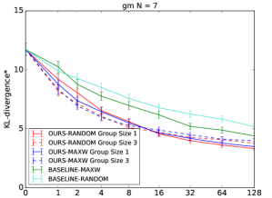
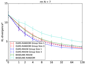
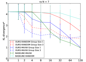
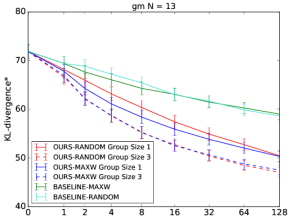
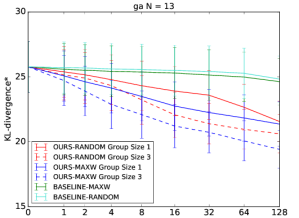
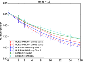
Mixed grid	Attractive grid	Mixed random	Attractive random

Figure 2: KL-divergence using either our clamping method or that of [37] averaged over 100 trials. The vertical bars represent standard deviations. Attractive means that pairwise terms are drawn uniformly from $[0,6]$ whereas Repulsive means drawn from $[-6,6]$. Grid indicates a grid topology for the CRF, whereas Random indicates that the connections are chosen randomly such that there are as many as in the grids. We ran our experiments with both $7\times 7$ and $13\times 13$ variables CRFs.

7.2 Multi-modal Probabilistic Occupancy Maps

The Probabilistic Occupancy Map (POM) method [13] relies on Mean Field inference for pedestrian detection. More specifically, given several cameras with overlapping fields of view of a discretized ground plane, the algorithm first performs background subtraction. It then estimates the probabilities of occupancy at every discrete location as the marginals of a product law minimizing the KL divergence from the “true” conditional posterior distribution, formulated as in Eq. 1 by defining an energy function. Its value is computed by using a generative model: It represents humans as simple cylinders projecting to rectangles in the various images. Given the probability of presence or absence of people at different locations and known camera models, this produces synthetic images whose proximity to the corresponding background subtraction images is measured and used to define the energy.

This algorithm is usually very robust but can fail when multiple interpretations of a background subtraction image are possible. This stems from the limited modeling power of the standard MF approximation, as illustrated in the supplementary material. We show here that, in such cases, replacing MF by MMMF while retaining the rest of the framework yields multiple interpretations, among which the correct one is usually to be found.

Fig. 3 depicts what happens when we replace MF by MMMF to approximate the true posterior, while changing nothing else to the algorithm. To generate new branches of the binary tree of Section 5, we find potential variables to clamp as described in Section 6. Among those, we clamp the one with the largest entropy gap—$\mathcal{H}(q^{T}_{i})-\mathcal{H}(q^{1}_{i})$, using the notations of Eq. 15—and its neighbors on the grid. When evaluating our cardinality constraint, we take $C$ to be 1, meaning that one branch of the tree corresponds to no one in the neighborhood of the selected location and the other to at least one person being present in this neighborhood. Since we typically create those locations by discretizing the ground plane into $10cm\times 10cm$ grid cells, this forces the two newly instantiated modes to be significantly different as opposed to featuring the same detection shifted by a few centimeters. In Fig. 3, we plot the results as dotted curves representing the MODA scores as functions of the distance threshold used to compute them [6]. In all cases, we used 4 modes for the MMMF approximation and followed the DivMBest evaluation metric [4] to produce a score by selecting among the 4 detection maps corresponding to each mode the one yielding the highest MODA score. This produces red dotted MMMF curves that are systematically above the blue dotted MF.

However, to turn this improvement into a practical technique, we need a way to choose among the 4 possible interpretations without using the ground truth. We use temporal consistency to jointly find the best sequence of modes, and reconstruct trajectories from this sequence. In the original algorithm, the POMs computed at successive instants were used to produce consistent trajectories using the a K-Shortest Path (KSP) algorithm [5]. This involves building a graph in which each ground location at each time step corresponds to a node and neighboring locations at consecutive time steps are connected. KSP then finds a set of node-disjoint shortest paths in this graph where the cost of going through a location is proportional to the negative log-probability of the location in the POM [33]. Since MMMF produces multiple POMs, we then solve a multiple shortest-path problem in this new graph, with the additional constraint that at each time step all the paths have to go through copies of the nodes corresponding to the same mode, as described in more details in the supplementary material.

The solid blue lines in Fig. 3 depict the MODA scores when using KSP and the red ones the multi-modal version, which we label as KSP^∗. The MMMF curves are again above the MF ones. This makes sense because ambiguous situations rarely persist for more than a few a frames. As a result, enforcing temporal consistency eliminates them.

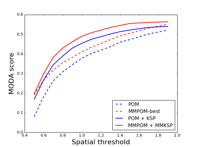
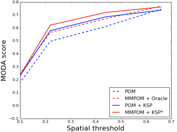
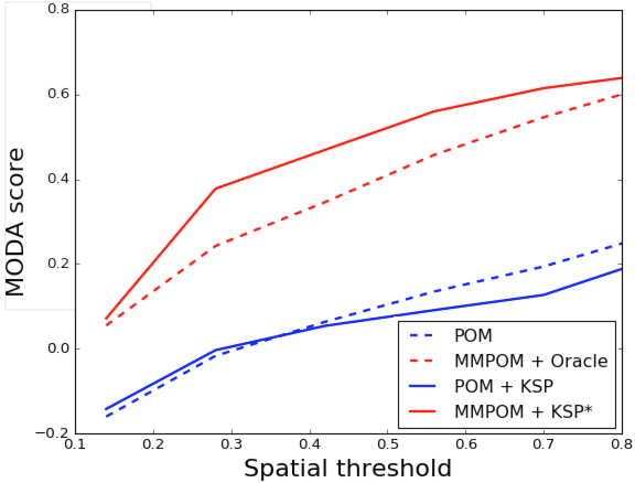
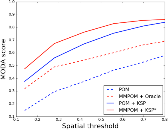
Figure 3: Replacing MF by MMMF in the POM algorithm [13]. The blue curves are MODA scores [6] obtained using MF and the red ones scores using MMMF. They are shown as solid lines when temporal consistency was enforced and as dotted lines otherwise. Note that the red MMMF lines are above corresponding blue MF ones in all cases. (a) 1000 frames from the MVL5 [26] dataset using a single camera. (b) 400 frames from the Terrace dataset [5] using two cameras. (c) 80 frames of the EPFL-Lab dataset [5] using a single camera. (d) 80 frames from the EPFL-Lab dataset [5] using two cameras.

7.3 Multi-Modal Semantic Segmentation

CRF-based semantic segmentation is one of best known application of MF inference in Computer Vision and many recent algorithms rely on dense CRF’s [23] for this purpose. We demonstrate here that our MMMF approximation can enhance the inference component of two such recent algorithms [9, 40] on the Pascal VOC 2012 segmentation dataset and the MPI video segmentation one  [15].

Individual VOC Images

We write the posterior in terms of the CRF of [9], which we try to approximate. To create a branch of the binary tree of Section 5, we first find the potential variables to clamp as described in Section 6. As in 7.2, we select the ones in the sliding window with the largest entropy gap, $\mathcal{H}(q^{T}_{i})-\mathcal{H}(q^{1}_{i})$. We then take $C$ to be $L/2$ when evaluating our cardinality constraint, meaning that we seek the dominant label among the selected variables and split the state space into those for which more than half these variables take this value and those in which less than half do.

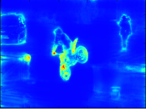
(a)	(b)
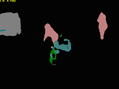
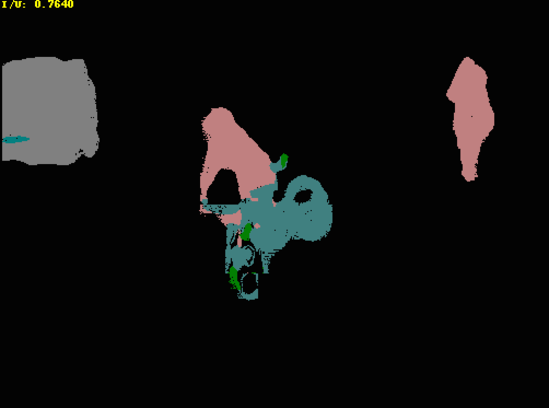
(c)	(d)

Figure 4: Qualitative semantic segmentation. (a) Original image. (b) Entropy gap. (c) Labels with maximum a Posteriori Probability after MF approximation. (d) Labels with maximum a Posteriori Probability for the best mode of the MMMF approximation.

Fig. 4 illustrates the results on an image of the VOC dataset. To evaluate such results quantitatively, we first use the DivMBest metric [4], as we did in Section 7.2. We assume we have an oracle that can select the best mode of our multi-modal approximation by looking at the ground truth. Fig. 5 depicts the results on the validation set of the VOC 2012 Pascal dataset in terms of the average intersection over union (IU) score as a function of the number of modes. When only 1 mode is used, the result boils down to standard MF inference as in [9]. Using 32 yields a $2.5\%$ improvement over the MF approximation. This may seem small until one considers that we only modify the algorithm’s inference engine and leave the unary terms unchanged. In [9, 41], this engine has been shown to contribute approximately $3\%$ to the overall performance, which means that we almost double its effectiveness. For analysis purposes, we implemented two baselines:

• Instead of clamping groups of variables, we only clamp the variable with the maximum entropy gap at each step. As depicted by the red curve in Fig. 5, this has absolutely no effect and illustrates the importance of clamping groups of variable instead of single ones as in [37].

• The DivMBest approach [4] first computes a MAP and then adds a penalty term to the energy function to find another MAP that is different from the first. It then repeats the process. We adapted this approach for MF inference. The green curve in Fig. 5 depicts the result, which MMMF outperforms by $1.5\%$.

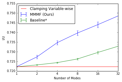
IU score for the best mode

Figure 5: Quantitative semantic segmentation on VOC 2012. IU score for best mode as a function of the number of modes. MMMF in blue, baselines in red and green.

Semantic Video Segmentation.

We ran the same experiment on the images of the MPI video segmentation dataset [15] using the CRF of [40]. In this case, we can exploit temporal consistency to avoid having to use an oracle and nevertheless get an exploitable result, as we did in Section 7.2. Furthermore, we can do this in spite of the relatively low frame-rate of about 1Hz.

More specifically, we first define a compatibility measure between consecutive modes based on label probabilities of matching key-points, which we compute using a key-point matching algorithm [30]. We then compute a shortest path over the sequence of modes, taking into account individual mode probabilities given by Eq. 11. Finally, we use only the MAP corresponding to the mode chosen by the shortest path algorithm to produce the segmentation. In Fig. 1, we again report the results in terms of IU score. This time the improvement is around $2.4\%$, which indicates that imposing temporal consistency very substantially improves the quality of the inference. To the best of our knowledge, other state of the art video semantic segmentation methods are not applicable for such image sequences. [17] requires non-moving scenes and a super-pixel decomposition, which prevents using all the dense CRF-based image segmentors. [24] was only applied to street scenes and requires a much higher frame rate to provide an accurate flow estimation.

Method	Mean IOU
MF	44.9%
[37] + Temp	44.9%
MMMF + Temporal	47.3%
MMMF-Best	53.2%

Table 1: Quantitative semantic segmentation MPI dataset [15].

8 Conclusion

We have shown that our MMMF aproach makes it possible to add structure to the standard MF approximation of CRFs and to increase the performance of algorithms that depend on it. In effect, our algorithm creates several alternative MF approximations with probabilities assigned to them, which effectively models complex situations in which more than one interpretation is possible.

Since MF has recently been integrated into structured learning architectures through the Back Mean-Field procedure [11, 25, 41, 1], future work will aim to replace MF by MMMF in this context as well.

Appendix A Proofs for Multi-Modal Mean-Fields via Cardinality-Based Clamping

This document provides technical details and proofs related to Section 5. We first prove the approximation of the KL-Divergence used in Eq. 9. Then, we show that the problem that we are trying to solve in Eq. 9, the minimization of the KL-Divergence, is actually equivalent to the one solved by [37], namely, finding an approximation to the log-partition function. It eventually justifies the benchmark experiments ran in 7.1. Finally, we justify the Gaussian approximation used in the case of large clamping groups in 5.2.1-(2).

A.1 Minimising the KL-Divergence

Let us see how the KL-Divergence between $Q_{MM}$ and P of Eq. 3 can be minimised with respect to the parameters $m_{k}$ and to the distributions $Q_{k}$, leading to Eq. 9. We reformulate the minimisation problem up to a constant approximation factor of order $\epsilon\log(\epsilon)$.

First, remember that our minimisation problem enforces the near-disjointness condition,

$$\forall k\neq k^{\prime}\sum_{\mathbf{x}\in\mathcal{X}_{k}^{\prime}}Q_{k}(\mathbf{x})\leq\epsilon\;,$$ (16)

between the elements of the mixture.

Let us then prove the following useful Lemma.

Lemma A.1

For all mixture element $k\leq K$,

$$\sum\limits_{\mathbf{x}\in\mathcal{X}}Q_{k}(\mathbf{x})\log\left(\sum\limits_{k^{\prime}\leq K}m_{k^{\prime}}Q_{k^{\prime}}(\mathbf{x})\right)=\sum\limits_{\mathbf{x}\in\mathcal{X}}Q_{k}(\mathbf{x})\log\left(m_{k}Q_{k}(\mathbf{x})\right)+\mathcal{O}(\epsilon\log\epsilon)\;.$$ (17)

• Let $k$ be the index of a mixture component $k\leq K$, and let us denote the approximation error

  $$\delta_{k}=\sum\limits_{\mathbf{x}\in\mathcal{X}}Q_{k}(\mathbf{x})\log\left(\sum\limits_{k^{\prime}\leq K}m_{k^{\prime}}Q_{k^{\prime}}(\mathbf{x})\right)-\sum\limits_{\mathbf{x}\in\mathcal{X}}Q_{k}(\mathbf{x})\log\left(m_{k}Q_{k}(\mathbf{x})\right)\;.$$ (18)

  Then, we use the near-disjointness condition to bound $\delta_{k}$,

  $$\delta_{k} \leq\underbrace{\sum\limits_{\mathbf{x}\in\mathcal{X}_{k}}Q_{k}(\mathbf{x})\log\left(1+\dfrac{\sum\limits_{k^{\prime}\neq k}m_{k^{\prime}}Q_{k^{\prime}}(\mathbf{x})}{Q_{k}(\mathbf{x})}\right)}_{I}+\underbrace{\sum\limits_{\mathbf{x}\in\mathcal{X}\setminus\mathcal{X}_{k}}Q_{k}(\mathbf{x})\log\left(1+\dfrac{\sum\limits_{k^{\prime}\neq k}m_{k^{\prime}}Q_{k^{\prime}}(\mathbf{x})}{Q_{k}(\mathbf{x})}\right)}_{J}$$ (19)

  We first use the well known inequality $\log(1+x)\leq x$ in order to upper bound $I$,

  $$I \leq\sum\limits_{\mathbf{x}\in\mathcal{X}_{k}}Q_{k}(\mathbf{x})\dfrac{\sum\limits_{k^{\prime}\neq k}m_{k^{\prime}}Q_{k^{\prime}}(\mathbf{x})}{Q_{k}(\mathbf{x})}$$ (20)

  $$\leq\sum\limits_{k^{\prime}\neq k}\sum\limits_{\mathbf{x}\in\mathcal{X}_{k}}m_{k^{\prime}}Q_{k^{\prime}}(\mathbf{x})$$ (21)

  $$\leq\sum\limits_{k^{\prime}\neq k}\epsilon$$ (22)

  $$\leq\mathcal{O}(\epsilon)\;.$$ (23)

  The second term, $J$, can then be upper-bounded using the fact that the $m_{k^{\prime}}$ and $Q_{k^{\prime}}$ are mixture weights and probabilities and hence $\sum\limits_{k^{\prime}\neq k}m_{k^{\prime}}Q_{k^{\prime}}(\mathbf{x})\leq 1$ for all $\mathbf{x}$. Therefore,

  $$J \leq\sum\limits_{\mathbf{x}\in\mathcal{X}\setminus\mathcal{X}_{k}}Q_{k}(\mathbf{x})\log\left(1+\dfrac{1}{Q_{k}(\mathbf{x})}\right)$$ (24)

  $$\leq\sum\limits_{\mathbf{x}\in\mathcal{X}\setminus\mathcal{X}_{k}}-Q_{k}(\mathbf{x})\log\left(Q_{k}(\mathbf{x})\right)$$ (25)

  $$\leq\sum\limits_{k^{\prime}\neq k}\sum\limits_{\mathbf{x}\in\mathcal{X}_{k^{\prime}}}-Q_{k}(\mathbf{x})\log\left(Q_{k}(\mathbf{x})\right)\;.$$ (26)

  Furthermore, for all $k^{\prime}\neq k$, the near-disjointness condition enforces that $\sum\limits_{\mathbf{x}\in\mathcal{X}_{k^{\prime}}}Q_{k}(\mathbf{x})\leq\epsilon$. Under this constraint, on each of the subsets $\mathcal{X}_{k^{\prime}}$, the maximal entropy is reached if $Q_{k}(\mathbf{x})=\dfrac{\epsilon}{\mid\mathcal{X}_{k^{\prime}}\mid}$ for all $\mathbf{x}$ in $\mathcal{X}_{k^{\prime}}$. And, therefore

  $$\sum\limits_{\mathbf{x}\in\mathcal{X}_{k^{\prime}}}-Q_{k}(\mathbf{x})\log\left(Q_{k}(\mathbf{x})\right) \leq\epsilon\log\left(\dfrac{\mid\mathcal{X}_{k}^{\prime}\mid}{\epsilon}\right)$$ (27)

  $$\leq\mathcal{O}(\epsilon\log\epsilon)+\mathcal{O}(\epsilon)\;,$$ (28)

  where the factor $\log(\mid\mathcal{X}_{k}\mid)$, which is of the order of the number of variables, has been integrated in the constant.

  Hence,

  $$J \leq\sum\limits_{k^{\prime}\neq k}\sum\limits_{\mathbf{x}\in\mathcal{X}_{k^{\prime}}}-Q_{k}(\mathbf{x})\log\left(Q_{k}(\mathbf{x})\right)$$ (29)

  $$\leq\mathcal{O}(\epsilon\log\epsilon)+\mathcal{O}(\epsilon)\;,$$ (30)

  which terminates the proof.

We can then move on to the minimisation of the KL-Divergence

$$\min\limits_{\hat{m},\hat{q}}\text{KL}(Q_{MM}\|P) =\min\limits_{\hat{m},\hat{q}}\sum\limits_{\mathbf{x}\in\mathcal{X}}\sum\limits_{k\leq K}Q_{MM}(\mathbf{x})\log\left(\dfrac{Q_{MM}(\mathbf{x})}{P(\mathbf{x})}\right)$$ (32)

$$=\min\limits_{\hat{m},\hat{q}}\sum\limits_{\mathbf{x}\in\mathcal{X}}\sum\limits_{k\leq K}Q_{MM}(\mathbf{x})\log\left(\dfrac{Q_{MM}(\mathbf{x})}{e^{-E(\mathbf{x})}}\right)+\log(Z)$$ (33)

$$=\min\limits_{\hat{m},\hat{q}}\sum\limits_{k\leq K}\sum\limits_{\mathbf{x}\in\mathcal{X}}m_{k}Q_{k}(\mathbf{x})\log\left(\dfrac{\sum\limits_{k^{\prime}\leq K}m_{k^{\prime}}Q_{k^{\prime}}(\mathbf{x})}{e^{-E(\mathbf{x})}}\right)+\log(Z)$$ (34)

$$=\min\limits_{\hat{m},\hat{q}}\sum\limits_{k\leq K}\sum\limits_{\mathbf{x}\in\mathcal{X}}m_{k}Q_{k}(\mathbf{x})\log\left(\dfrac{m_{k}Q_{k}(\mathbf{x})}{e^{-E(\mathbf{x})}}\right)+\log(Z)+\mathcal{O}(\epsilon\log\epsilon)$$ (35)

$$=\min\limits_{\hat{m}}\left[\sum\limits_{k\leq K}m_{k}\log m_{k}+\sum\limits_{k\leq K}\min\limits_{q_{k}}\sum\limits_{\mathbf{x}\in\mathcal{X}}m_{k}Q_{k}(\mathbf{x})\log\left(\dfrac{Q_{k}(\mathbf{x})}{e^{-E(\mathbf{x})}}\right)\right]+\log(Z)+\mathcal{O}(\epsilon\log\epsilon)$$ (36)

$$=\min\limits_{\hat{m}}\sum\limits_{k\leq K}m_{k}\log(m_{k})-\sum\limits_{k\leq K}m_{k}A_{k}+\log(Z)+\mathcal{O}(\epsilon\log\epsilon)\;,$$ (37)

where,

$$A_{k} =\max\limits_{q^{k}_{i},{i=1\dots N}}\sum\limits_{\mathbf{x}\in\mathcal{X}}Q_{k}(\mathbf{x})\log\left(\dfrac{e^{-E(\mathbf{x})}}{Q_{k}(\mathbf{x})}\right)\;.$$

Equation 35 is obtained using Lemma A.1.

Assuming that we are able to compute $A_{k}$, for all $k$, the minimisation of this KL-Divergence with respect to parameters $m_{k}$, under the nomalisation constraint

$$\sum\limits_{k\leq K}m_{k}=1\;,$$ (38)

is then straightforward and leads to

$$m_{k}=\dfrac{e^{A_{k}}}{\sum\limits_{k^{\prime}\leq K}e^{A_{k^{\prime}}}}\;.$$ (39)

A.2 Equivalence with the approximation of the partition function.

The recent work of [37], that we use as a baseline, looks for the best heuristic to choose the clamping variables. They measure the quality of the approximation through the closeness of the estimated partition function, which they compute as the sum of MF approximated partition functions for each component of the mixture, to the true one. We will now see that this problem is strictly equivalent to the minimisation of the KL-Divergence of Eq. 9.

Indeed, replacing 38 in 37, we directly obtain that

$$\text{KL}(Q_{MM}\|P) =\log(\sum\limits_{k^{\prime}\leq K}e^{A_{k^{\prime}}})+\log(Z)+\mathcal{O}(\epsilon\log\epsilon)$$ (40)

$$=\log(Z)-\log(\tilde{Z})+\mathcal{O}(\epsilon\log\epsilon)\;,$$ (41)

where,

$$\tilde{Z}=\sum\limits_{k^{\prime}\leq K}e^{A_{k^{\prime}}}\;,$$ (42)

is precisely the approximation of the partition function $Z$ proposed by [37]. In other terms, it is the sum of local variational lower-bounds on clamped subsets of the state space.

A.3 Gaussian approximation to the cardinality constraint.

In the following, we explain the Gaussian approximation of the cardinality constraint used in 5.2.1-(2) and in our application to Semantic Segmentation. Let us consider the case where we generate only two modes modelled by $Q_{1}(\mathbf{x})=\prod q^{1}_{i}(x_{i})$ and $Q_{2}(\mathbf{x})=\prod q^{2}_{i}(x_{i})$ and we seek to estimate the $q^{1}_{i}$ probabilities. The $q^{2}_{i}$ probabilities are evaluated similarly.

Recall that, each $A_{k}$ is obtained through the constrained MF optimisation problem

$$\max\limits_{q^{k}_{i},{i=1\dots N}} \sum\limits_{\mathbf{x}\in\mathcal{X}}Q_{k}(\mathbf{x})\log\left(\dfrac{e^{-E(\mathbf{x})}}{Q_{k}(\mathbf{x})}\right)$$ (43)

s.t. $$Q_{1}\left(\sum\limits_{u=1\dots L}\mathbbm{1}(\mathbf{X}_{i_{u}}=v_{u})<C\right)\leq\epsilon\;.$$

Under the probability $Q_{1}$, $\sum\limits_{u=1\dots L}\mathbbm{1}(\mathbf{X}_{i_{u}}=v_{u})$ is a sum of independent binary random variables that are non identically distributed, in other words, a Poisson Binomial Distribution. In the general case, there is no closed-form formula for computing the Cumulative Distribution Function of such a distribution from the individual marginals parametrising $Q_{1}$. However, when $L$ is large ($\geq 10$), the Gaussian approximation is good enough.

Therefore, we use a Gaussian approximation to replace the cardinality constraint by

$$\sum\limits_{u\in\{1\dots L\}}q^{1}_{i_{u}}(v_{u})<C+\sigma F^{-1}(1-\epsilon)\;,$$ (44)

where $F$ is the Gaussian cumulative distribution fonction and $\sigma^{2}$ the variance, which, in theory should be

$$\sigma^{2}=\sum\limits_{u\in\{1\dots L\}}q^{1}_{i_{u}}(v_{u})(1-q^{1}_{i_{u}}(v_{u}))\;,$$ (45)

but which can be either upper-bounded by $\dfrac{L}{4}$ or re-estimated at the beginning of each Lagrangian iteration.

In short, we replace the untractable higher order constraint LABEL:eq:constrainedOptim, by a simple one involving only the sum of the MF parameters $q^{1}_{i_{u}}(v_{u})$.

Appendix B Computing the Critical Temperature for the Dense Gaussian CRFs

We first compute analytically the phase transition temperature parameter $T_{c}$ of 6.2 where the KL-Divergence stops being convex. In the first part Analytical Derivation, we make strong assumptions in order to be able to obtain a closed form estimation of $T_{c}$. We then explain how this result helps understanding real cases. In the second part Experimental Analysis, in order to justify our assumptions, we run experiments under three regimes, one where our assumptions are strictly verified, one which corresponds to a real-life scenario and an intermediate one. This set of experiments shows that our strong assumptions provide a valuable insight for practical applications.

B.1 Analytical derivation

Let us take probability distribution $P$ to be defined by a dense Gaussian CRF [23]. In order to make computation tractable, we assume that the RGB distance between pixels is uniform and equal to $d_{rgb}$. Therefore the RGB Kernel is constant with value

$$\theta_{rgb}=e^{\dfrac{-d_{rgb}^{2}}{2\sigma_{rgb}}}\;.$$ (46)

We consider the case where we have only two possible labels and the same unary potential on all the variables. Even if this assumption sounds strong, we can expect them to be locally valid. Formally, on a $N\times N$ dense grid, the energy function is defined as

$$E(\mathbf{x}) =\dfrac{\Gamma\theta_{rgb}}{2\pi\sigma^{2}}\sum\limits_{(i,j),(i^{\prime},j^{\prime})}\mathbbm{1}[\mathbf{x}_{(i,j)}\neq\mathbf{x}_{(i^{\prime},j^{\prime})}]e^{-\dfrac{\|(i,j)-(i^{\prime},j^{\prime})\|^{2}}{2\sigma}}$$

$$+\sum\limits_{(i,j)}U_{(i,j)}\mathbbm{1}[\mathbf{x}_{(i,j)}=0]\;,$$

where $\sigma$ controls the range of the correlations and $U_{(i,j)}$ is a unary potential.

Since that we assumed that all the variables receive the same unary $U$, all the variables are undiscernibles. Furthermore, the pairwise potentials are attractive, we therefore expect all the mean-field parameters $q_{i,j}=Q(\mathbf{x}_{i,j}=0)$ to have the same value at the fixed point solution of the Mean-Field. Therefore, we designate this common parameter $q^{T}$ and we can try to find analytically the Mean-Field fixed point for $q^{T}$ corresponding to a temperature $T$.

At convergence, the parameter $q^{T}$ will have to satisfy

$$\log(q^{T}) =\mathbb{E}_{Q}(E(\mathbf{x})|x_{i}=0)$$

$$=-\dfrac{\Gamma\theta_{rgb}}{2\pi\sigma^{2}T}\sum\limits_{(i,j)\in\mathbb{Z}\times\mathbb{Z}}(1-q^{T})e^{-\dfrac{\|(i,j)\|^{2}}{2\sigma}}-\dfrac{U}{T}$$

$$=-\dfrac{(1-q^{T})\Gamma\theta_{rgb}+U}{T}$$

Hence, we obtain the fixed point equation

$$\tilde{q}^{T}=\dfrac{1}{2}\tanh\left({\dfrac{\tilde{q}^{T}\Gamma\theta_{rgb}-U}{T}}\right)\;,$$ (47)

where $\tilde{q}^{T}=q^{T}-0.5$. As depicted in Figure 6, when unaries are 0 (on the left) there are two distinct regimes for the solutions of this equation. For high $T$, there is only one stable solution at $\tilde{q}=0$. For low $T$, there are two distinct stable solutions where $\tilde{q}$ is close to $-0.5$ or $0.5$. The temperature threshold $T_{c}$ where the transition happens, corresponds to the solution of

$$\dfrac{1}{2}\dfrac{d\tanh(\dfrac{\tilde{q}\Gamma\theta_{rgb}}{T})}{d\tilde{q}}|_{\tilde{q}=0}=1\;,$$ (48)

and hence $T_{c}=\dfrac{\Gamma\theta_{rgb}}{2}$. For real images, we have $\theta_{rgb}\leq 1$, and therefore, $T_{c}=\dfrac{\Gamma}{2}$ can be used to upper-bound the true critical temperature.

When unaries are non-zero, there is no closed form solution for $T_{c}$, however, from Equation 47, we can show that the smaller the unaries ($U$), the lower the critical temperature will be. This is intuitively justified in Fig. 6.

The authors of [37], use several heuristics which basically consist in looking for high correlations and low unaries directly in the potentials of the graphical model, in order to find good variables to clamp. We, instead use a criterium based on the critical temperature in order to spot these.

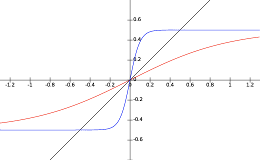
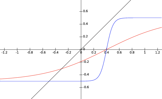
Without unaries	With unaries

Figure 6: $\tanh(\dfrac{\tilde{q}\Gamma-U}{T})$ for two temperatures. Low T (blue) and High T (red).

B.2 Experimental analysis

We use the dense CRF implementation of [23] to verify the phase transition experimentally for $\Gamma=10$. In our experiments, we used the three following settings, which range from the stylised example used for calculation to real semantic segmentation problems:

• Model 1: We use a uniform rgb image $d_{rgb}=0$. Two classes without unary potentials. This is exactly the model used for the derivations with $\theta_{rgb}=1$ and $U=0$.

• Model 2: Gaussian potentials defined over image coordinates distance + RGB distance. Two classes without unary potentials. In other words, $\theta_{rgb}\leq 1$.

• Model 3: Gaussian potentials defined over image coordinates distance + RGB distance. Two classes with unary potentials produced by a CNN. This is a real-life scenario.

Fig. 7 shows that, as expected, two regimes appear for Model 1, before and after $T=5$. We see that our prediction remains completely valid for Model 2, some non-uniform regions fall under the regime $\theta_{rgb}\leq 1$ and therefore the 10 % highest entropy percentile transitions slightly earlier. For Model 3, however, we see that the minimal and average entropy remain low even for $T>5$. This is well explained by the fact that large regions of the image receive strong unary potentials from one class or the other, and therefore fall under the case ”with unaries” of Fig. 6 where the $U$ parameter cannot be ignored. However, some uncertain regions receive unary potentials of same value for both labels, and therefore undergo a phase transition as predicted by our calculation. That is why the maximal entropy behaves similarly to Model 2. Our algorithm precisely targets these uncertain regions.

Interestingly, we see that in practice, the users of DenseCRF choose the $\Gamma$ and $T$ parameters in order to be in a Multi-Modal regime, but close to the phase transition. For instance in the public releases of [9] and  [41], the Gaussian kernel is set with $T=1$ and $\Gamma=3$.

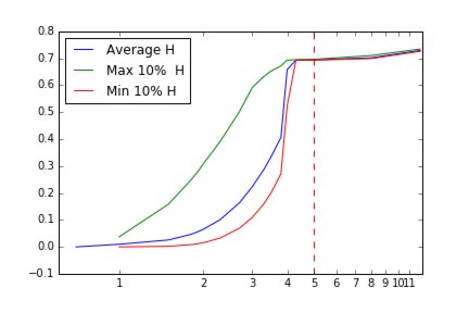
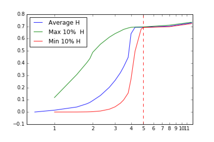
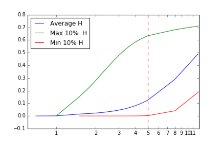
Model 1	Model 2	Model 3

Figure 7: Entropy as a function of temperature.

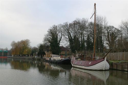
RGB Image

Model 1

Model 2

Model 3

Figure 8: Evolution of MF probability for background label when temperature increases

Appendix C K-Shortest Path algorithm for the Multi-Modal Probabilistic Occupancy Maps

We present here the algorithm we use to reconstruct tracks from the Multi-Modal Probabilistic Occupancy Maps (MMPOMs) of Section 7.2.

KSP

In the original algorithm of [5], the POMs computed at successive instants were used to produce consistent trajectories using the a K-Shortest Path (KSP) algorithm [33]. This involves building a graph in which each ground location at each time step corresponds to a node and neighboring locations at consecutive time steps are connected. KSP then finds a set of node-disjoint shortest paths in this graph where the cost of going through a location is proportional to the negative log-probability of the location in the POM [5]. The KSP problem can be solved in linear time and an efficient implementation is available online.

KSP for Multi-Modal POM

Since MMMF produces multiple POMs, one for each mode, at each time-step, we duplicate the KSP graph nodes, once for each mode as well. Each node is then connected to each copy of neighboring locations from previous and following time steps. We then solve a multiple shortest-path problem in this new graph, with the additional constraint that at each time step all the paths have to go through copies of the nodes corresponding to the same mode. This larger problem is NP-Hard and cannot be solved by a polynomial algorithm such as KSP. We therefore use the Gurobi Mixed-Integer Linear Program solver [16].

More precisely, let us assume that we have a sequence of Multi-Modal POMs $Q^{t}_{k}$ and mode probabilities $m^{t}_{k}$ for $t\in\{1,\dots,T\}$ representing time-steps and $k\in\{1,\dots,K\}$ representing different modes. Each $Q^{t}_{k}$ is materialized through a vector of probabilities of presence $q^{t}_{k,i}$, where each $i\leq N$ is indexes a location on the tracking grid.

Using the grid topology, we define a neighborhood around each variable, which corresponds to the maximal distance a walking person can make on a grid in one time step. Let us denote by $\mathcal{N}_{i}$ the set of indices corresponding to locations in the neighbourhood of $i$. The topology is fixed and hence $\mathcal{N}_{i}$ does not depend on the time steps. We define the following log-likelihood costs.

Using a Log-Likelihood penalty, we define the following costs:

• $C^{t}_{k,i}=\log\left(\dfrac{1-q^{t}_{k,i}}{q^{t}_{k,i}}\right)$, representing the cost of going through variable $i$ at time $t$ if mode $k$ is chosen.

• $C^{t}_{k}=\log\left(\dfrac{1-m^{t}_{k}}{m^{t}_{k}}\right)$, representing the cost of choosing mode $k$ at time $t$.

We solve for an optimization problem involving the following variables:

• $x^{t}_{k,i,l,j}$ is a binary flow variable that should be $1$ if a person was located in $i$ at $t$ and moved to $j$ at $t+1$, while modes $k$ and $l$ were respectively chosen at time $t$ and $t+1$.

• $y^{t}_{k}$ is a binary variable that indicates whether mode $k$ is selected at time $t$.

We can then rewrite the Multi-Modal K-Shortest Path problem as the following program, were we always assume that $t\leq T$ stands for a time step, $k\leq K$ and $l\leq K$ stand for mode indices, and $i\leq N$ and $j\leq N$ stand for grid locations:

$$\min \sum\limits_{t,k}C^{t}_{k}y^{t}_{k}+\sum\limits_{t,k,l\leq K}\sum\limits_{i,j\in\mathcal{N}_{i}}C^{t}_{k,i}x^{t}_{k,i,l,j}$$ (49)

s.t. $$\forall(t,k,i)\;,\;\;\sum\limits_{l,j\in\mathcal{N}_{i}}x^{t-1}_{l,j,k,i}=\sum\limits_{l,j\in\mathcal{N}_{i}}x^{t}_{k,i,l,j}$$ flow conservation

$$\forall(t,k,i)\;,\;\;\sum\limits_{l,j\in\mathcal{N}_{i}}x^{t}_{k,i,l,j}\leq y^{t}_{k}$$ disjoint paths + selected mode

$$\forall t\;,\;\;\sum\limits_{k}y^{t}_{k}=1$$ selecting one mode

$$\forall t,k,i,l,j\;,\;\;0\leq x^{t}_{k,i,l,j}\leq 1\;$$

$$\forall t,k\;,\;\;y^{t}_{k}\in\{0,1\}\;$$

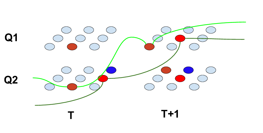
Figure 9: Illustration of the output of our K-Shortest Path algorithm in the case of multiple modes.

KSP prunning

However, the problem as written above, may involve several tens millions of flow variables and therefore becomes intractable, even for the best MILP solvers. We therefore first prune the graph to drastically reduce its size.

The obvious strategy would be by thresholding the POMs and removing all the outgoing and incoming edges from locations which have probabilities below $q_{thresh}$. However, this would be self-defeating as one of the main strengths of the KSP formulation is to be very robust to missing-detections and be able to reconstruct a track even if a detection is completely lost for several frames.

We therefore resort to a different strategy. More precisely, we initially relax the constraint disjoint paths + selected mode, to a simple disjoint path constraint, and remove the constraint selecting one mode. We therefore obtain a relaxed problem

$$\min \sum\limits_{t,k}\sum\limits_{t,k,l\leq K}\sum\limits_{i,j\in\mathcal{N}_{i}}C^{t}_{k,i}x^{t}_{k,i,l,j}$$ (50)

s.t. $$\forall(t,k,i)\;,\;\;\sum\limits_{l,j\in\mathcal{N}_{i}}x^{t-1}_{l,j,k,i}=\sum\limits_{l,j\in\mathcal{N}_{i}}x^{t}_{k,i,l,j}$$ flow conservation

$$\forall(t,k,i)\;,\;\;\sum\limits_{l,j\in\mathcal{N}_{i}}x^{t}_{k,i,l,j}\leq 1$$ disjoint paths

$$\forall t,k,i,l,j\;,\;\;0\leq x^{t}_{k,i,l,j}\leq 1\;$$

which is nothing but a vanilla K-Shortest Path Problem. It can be solved using our linear-time KSP algorithm. This KSP problem will output a very large number of paths, going through all the different modes simultaneously. From, this output, we extract the set of grid locations which are used, in any mode, at each time step, and select them as our potential locations in the final program. In our current implementation, we add to these locations, the ones for which $q^{t}_{k,i}\geq q_{thresh}$ for any mode at time-step $t$.

We can finally solve Program LABEL:eq:MILP, where non-selected locations are pruned from the flow graph. We don’t know if our strategy, based on a relaxation and pruning, provides a guaranteed optimal solution to LABEL:eq:MILP, but this is an interesting question.

Appendix D Pseudo-code for the Multi-Modal Mean-Fields algorithm

Algorithm 1 summarises the operations to split one mode into two, or, in other words, to obtain the two additional constraints which are used to define the two newly created subsets. Algorithm 2 summarises the operations to obtain the Multi-Modal Mean Field Distribution by constructing the whole Tree.

In Algorithm 2, $ConstraintTree$, is taken to be a Tree in the form of a list of constraints, one for each branching-point, or leaf,—except for the root—, in a breadth first order. The function $\texttt{pathto}(nNode)$, returns the set of indices corresponding to the branching points on the path to the branching point, or leaf with index $nNode$, including index $nNode$ itself.

Algorithm 1 Function:$\texttt{Split}(ConstraintList)$

Input:
$E(\mathbf{x})$: An Energy function defined by a CRF;
$\texttt{SolveMF}(E,ConstraintList)$: A Mean Field solver with cardinality constraint.;
$Temperatures$: A list of temperatures in increasing order;
$\mathcal{H}_{low},\mathcal{H}_{high}$: Entropy thresholds for the phase transition. 0.3 and 0.6 here.
$C$: A cardinality threshold
Output:
$LeftConstraints$: A triplet containing a list of variables, clamped to value, -C
$RightConstraints$: A triplet containing a list of variables, clamped to value, C

  $Q^{T_{0}}\leftarrow\texttt{SolveMF}(E)$

  for $\texttt{T in }Temperatures$ do

     $Q^{T}\leftarrow\texttt{SolveMF}(\dfrac{E}{T},ConstraintList)$

     $i_{list}\leftarrow[.]$

     $v_{list}\leftarrow[.]$

     for index in $1\dots\texttt{len}(Q^{t})$, v in $labels$ do

        if $\mathbbm{1}[\mathcal{H}(q^{T}_{index})>0.6]\mathbbm{1}[\mathcal{H}(q^{T_{0}}_{index})<0.3]\mathbbm{1}[q^{T_{0}}_{index,v}>0.5]=1$ then

           $i_{list}$.append(index),$v_{list}$.append(v)

        end if

     end for

     if $\texttt{len}(i_{list})>0$ then

        exit for loop

     end if

  end for

  $LeftConstraints$ = $i_{list},v_{list},-C$

  $RightConstraints$ = $i_{list},v_{list},C$

  return  $LeftConstraints$,$RightConstraints$

Algorithm 2 Compute Multi-Modal Mean Field

Input:
$E(\mathbf{x})$: An Energy function defined on a CRF;
$\texttt{SolveMF}(E,ConstraintList)$: A Mean Field solver with cardinality constraint;
$\texttt{Split}(ConstraintList)$: Alg. 1. A function that computes the new constraints.
$NModes$: A target for the number of modes in the Multi-Modal Mean Field
Output:
$Qlist$: A list of Mean Field distributions in the form of a table of marginals
$mlist$: A list of probabilities, one for each mode

  $ConstraintTree=[.]$ We first build the tree by adding constraints.

  while $nNode<NModes$ do

     $ConstraintList=[.]$

     for $p\texttt{ in pathto}(nNode)$ do

        $ConstraintList$.append(ConstraintTree[p])

     end for

     $LeftConstraints,RightConstraints\leftarrow\texttt{Split}(ConstraintList)$

     $ConstraintTree$.append($LeftConstraints$)

     $ConstraintTree$.append($RightConstraints$)

  end whileWe now turn to the computation of on MF distribution per leaf.

  $Qlist=[.],Zlist=[.],mlist=[.]$

  for mode in $0\dots NModes$ do

     $ConstraintList=[.]$

     for $p\texttt{ in pathto}(mode+NModes-1)$ do

        $ConstraintList$.append(ConstraintTree[p])

     end for

     Q,Z $\leftarrow$ SolveMF(E,ConstraintList)

     $Qlist.\texttt{append}(Q)$

     $Zlist.\texttt{append}(Z)$

  end forFinally, we compute the mode probabilities.

  for $mode$ in $0\dots NModes$ do

     $mlist.\texttt{append}(\dfrac{Zlist[mode]}{\sum Zlist})$

  end for

  return  $Qlist$, $mlist$

References

- [1] A. Arnab, S. Jayasumana, S. Zheng, and P. H. S. Torr. Higher order potentials in end-to-end trainable conditional random fields. CoRR, abs/1511.08119, 2015.
- [2] T. Bagautdinov, P. Fua, and F. Fleuret. Probability Occupancy Maps for Occluded Depth Images. In Conference on Computer Vision and Pattern Recognition, 2015.
- [3] P. Baque, T. Bagautdinov, F. Fleuret, and P. Fua. Principled Parallel Mean-Field Inference for Discrete Random Fields. In Conference on Computer Vision and Pattern Recognition, 2016.
- [4] D. Batra, P. Yadollahpour, A. Guzman-Rivera, and G. Shakhnarovich. Diverse M-Best Solutions in Markov Random Fields. In European Conference on Computer Vision, pages 1–16, 2012.
- [5] J. Berclaz, F. Fleuret, E. Türetken, and P. Fua. Multiple Object Tracking Using K-Shortest Paths Optimization. IEEE Transactions on Pattern Analysis and Machine Intelligence, 33(11):1806–1819, 2011.
- [6] K. Bernardin and R. Stiefelhagen. Evaluating Multiple Object Tracking Performance: the Clear Mot Metrics. EURASIP Journal on Image and Video Processing, 2008, 2008.
- [7] A. Bouchard-Côté and M. I. Jordan. Optimization of structured mean field objectives. In Proceedings of the Twenty-Fifth Conference on Uncertainty in Artificial Intelligence, UAI ’09, pages 67–74, Arlington, Virginia, United States, 2009. AUAI Press.
- [8] S. Boyd and L. Vandenberghe. Convex Optimization. Cambridge University Press, 2004.
- [9] L.-C. Chen, G. Papandreou, I. Kokkinos, K. Murphy, and A. Yuille. Semantic Image Segmentation with Deep Convolutional Nets and Fully Connected CRFs. In International Conference for Learning Representations, 2015.
- [10] W.-H. Cho, S.-H. Kim, S.-Y. Park, and J.-H. Park. Mean field annealing em for image segmentation. In Image Processing, 2000. Proceedings. 2000 International Conference on, volume 3, pages 568–571 vol.3, 2000.
- [11] J. Domke. Learning Graphical Model Parameters with Approximate Marginal Inference. CoRR, abs/1301.3193, 2013.
- [12] F. Eaton and Z. Ghahrmani. Choosing a variable to clamp: Approximate inference using conditioned belief propagation. In International Conference on Artificial Intelligence and Statistics, 2009.
- [13] F. Fleuret, J. Berclaz, R. Lengagne, and P. Fua. Multi-Camera People Tracking with a Probabilistic Occupancy Map. IEEE Transactions on Pattern Analysis and Machine Intelligence, 30(2):267–282, February 2008.
- [14] R. Fransens, C. Strecha, and L. Van Gool. A Mean Field EM-Algorithm for Coherent Occlusion Handling in Map-Estimation Prob. In Conference on Computer Vision and Pattern Recognition, 2006.
- [15] F. Galasso, N. Nagaraja, T. Cardenas, T. Brox, and B.Schiele. A Unified Video Segmentation Benchmark: Annotation, Metrics and Analysis. In International Conference on Computer Vision, December 2013.
- [16] I. Gurobi Optimization. Gurobi optimizer reference manual, 2016.
- [17] J. Hur and S. Roth. Joint Optical Flow and Temporally Consistent Semantic Segmentation. CoRR, abs/1607.07716, 2016.
- [18] L. P. Kadanoff. More is the same; phase transitions and mean field theories. Journal of Statistical Physics, 137(5):777, 2009.
- [19] J. H. Kappes, B. Andres, F. A. Hamprecht, C. Schnörr, S. Nowozin, D. Batra, S. Kim, B. X. Kausler, T. Kröger, J. Lellmann, et al. A comparative study of modern inference techniques for structured discrete energy minimization problems. International Journal of Computer Vision, 115(2):155–184, 2015.
- [20] A. Kirillov, B. Savchynskyy, D. Schlesinger, D. Vetrov, and C. Rother. Inferring m-best diverse labelings in a single one. In Proceedings of the 2015 IEEE International Conference on Computer Vision (ICCV), ICCV ’15, pages 1814–1822, Washington, DC, USA, 2015. IEEE Computer Society.
- [21] P. Kohli and C. Rother. Higher-Order Models in Computer Vision. In O. Lezoray and L. Grady, editors, Image Processing and Analysis with Graphs, pages 65–100. CRC Press, 2012.
- [22] D. Koller and N. Friedman. Probabilistc Graphical Models. The MIT Press, 2009.
- [23] P. Krähenbühl and V. Koltun. Parameter Learning and Convergent Inference for Dense Random Fields. In International Conference on Machine Learning, pages 513–521, 2013.
- [24] A. Kundu, V. Vineet, and V. Koltun. Feature Space Optimization for Semantic Video Segmentation. In Conference on Computer Vision and Pattern Recognition, pages 1–8, 2016.
- [25] Y. Li and R. S. Zemel. Mean Field Networks. In International Conference on Machine Learning, 2014.
- [26] R. Mandeljc, S. K. M. Kristan, and J. Perš. Tracking by Identification Using Computer Vision and Radio. Sensors, 2012.
- [27] S. Nowozin, C. Rother, S. Bagon, T. Sharp, B. Yao, and P. Kholi. Decision Tree Fields. In International Conference on Computer Vision, November 2011.
- [28] E. Premachandran, D. Tarlow, and D. Batra. Empirical Minimum Bayes Risk Prediction: How to Extract an Extra Few % Performance from Vision Models with Just Three More Parameters. In Conference on Computer Vision and Pattern Recognition, June 2014.
- [29] V. Ramakrishna and D. Batra. Mode-Marginals: Expressing Uncertainty via Diverse M-Best Solutions. Advances in Neural Information Processing Systems, 2012.
- [30] J. Revaud, P. Weinzaepfel, Z. Harchaoui, and C. Schmid. Deepmatching: Hierarchical deformable dense matching. International Journal of Computer Vision, 120(3):300–323, 2016.
- [31] M. Saito, T. Okatani, and K. Deguchi. Application of the Mean Field Methods to MRF Optimization in Computer Vision. In Conference on Computer Vision and Pattern Recognition, June 2012.
- [32] L. Saul and M. I. Jordan. Exploiting Tractable Substructures in Intractable Networks. In Advances in Neural Information Processing Systems, pages 486–492, 1995.
- [33] J. W. Suurballe. Disjoint Paths in a Network. Networks, 4:125–145, 1974.
- [34] V. Vineet, G. Sheasby, J. Warrell, and P. H. S. Torr. Posefield: An efficient mean-field based method for joint estimation of human pose, segmentation, and depth. In A. Heyden, F. Kahl, C. Olsson, M. Oskarsson, and X.-C. Tai, editors, EMMCVPR, volume 8081 of Lecture Notes in Computer Science, pages 180–194. Springer, 2013.
- [35] V. Vineet, J. Warrell, and P. Torr. Filter-Based Mean-Field Inference for Random Fields with Higher-Order Terms and Product Label-Spaces. International Journal of Computer Vision, 110(3):290–307, 2014.
- [36] C. Wang, N. Komodakis, and N. Paragios. Markov Random Field Modeling, Inference & Learning in Computer Vision & Image Understanding: A Survey. Computer Vision and Image Understanding, 117(11):1610–1627, 2013.
- [37] A. Weller and J. Domke. Clamping improves trw and mean field approximations. In Advances in Neural Information Processing Systems, 2015.
- [38] A. Weller and T. Jebara. Approximating the bethe partition function. In Uncertainty in Artificial Intelligence, 2014.
- [39] P. Yadollahpour, , D. Batra, and B. Shakhnarovich. Discriminative Re-Ranking of Diverse Segmentations. In Conference on Computer Vision and Pattern Recognition, 2013.
- [40] F. Yu and V. Koltun. Multi-scale context aggregation by dilated convolutions. In ICLR, 2016.
- [41] S. Zheng, S. Jayasumana, B. Romera-paredes, V. Vineet, Z. Su, D. Du, C. Huang, and P. Torr. Conditional Random Fields as Recurrent Neural Networks. In International Conference on Computer Vision, 2015.