Universality and Asymptotic Scaling in Drilling Percolation

Abstract

We present simulations of a 3-d percolation model studied recently by K.J. Schrenk et al. [Phys. Rev. Lett. 116, 055701 (2016)], obtained with a new and more efficient algorithm. They confirm most of their results in spite of larger systems and higher statistics used in the present paper, but we also find indications that the results do not yet represent the true asymptotic behavior. The model is obtained by replacing the isotropic holes in ordinary Bernoulli percolation by randomly placed and oriented cylinders, with the constraint that the cylinders are parallel to one of the three coordinate axes. We also speculate on possible generalizations.

In spite of its mature age, the theory of percolation is still full of surprises Araujo . A new page was turned open recently by Schrenk et al. Schrenk , who revisited a model that was first studied long ago by Kantor Kantor . While Kantor had concluded that it was in the universality class of ordinary 3-d percolation, the simulations in Schrenk clearly suggest that it is in a different universality class. But these simulations also indicate very large corrections to scaling. Since the simulations were done on systems with rather modest sizes and did not use extremely large statistics, we decided to perform larger simulations in order to check their claims. The result can be summarized easily: Although our estimates of critical parameters are significantly more precise than those of Schrenk (and of course also of Kantor ), we fully confirm their main results. But we also find indications that these might not represent the true asymptotic behavior, which then would be even more different from ordinary percolation.

The model studied in Kantor ; Schrenk , called “drilling percolation” in the following, is very simple. Take a large solid block of size $L\times L\times L$ with $L\gg 1$ on a simple cubic lattice, and remove randomly columns of size $1\times 1\times L$, located randomly in the cube and oriented randomly but aligned with one of the three axes. The maximal number of columns is $3\times L\times L$ (each column of fixed orientation can be in one of $L\times L$ positions, and there are three orientations). The control parameter is defined as

$$p=\frac{\text{number of columns {\it not} taken out}}{3L^{2}}.$$ (1)

Notice that this is not the fraction of retained sites, since one site can be in two or even three columns. Nevertheless we expect qualitatively the same behavior as for ordinary site (“Bernoulli”) percolation: While the non-removed parts percolate for $p=1$, they cannot percolate for $p=0$, and there must be a critical point $p_{c}$ in between.

The non-trivial aspect of the model is that it involves geometric objects of more than one non-trivial dimensionality. While the bulk is three dimensional, the columns (holes) have $d=1$. Thus we expect that the standard field theory for percolation Amit cannot be applied without modifications. It is in this respect similar to models with long range correlations in the disorder Weinrib , of which it is indeed a special and particularly simple case.

The simulations were done in Schrenk by means of two different algorithms, both of which seem however to be less than optimal. In the present paper we shall use instead a very simple and efficient generalization of the well known Leath algorithm Leath for site percolation.

The latter is a cluster growth algorithm that uses two data structures: (i) a bit map, where for each site $(i,j,k)$ of the lattice it is stored whether it had been tested ($s_{ijk}=1$) or not yet ($s_{ijk}=0$); and (ii) a queue or stack (depending on whether it is implemented breadth first or depth first Cormen ) that contains a list of “growth sites”, i.e. sites that had recently be “wetted” (i.e., included in the cluster) and whose neighbors have to be tested whether they can be wetted or not. Notice that the bit map $s$ does not need to distinguish for tested sites whether the test had been positive (i.e. they were wetted) or not, as no site can be wetted later, if the first test was negative (this distinguishes site from bond percolation). Time in this growth process is discrete, if the difference between the times when a site gets wetted and wets itself its neighbors is defined as one unit of time.

In our generalization we have to add three more arrays $X_{jk}$, $Y_{ik}$ and $Z_{ij}$ of sizes $L\times L$ each, the elements of which can assume three possible values. $X_{jk}=0$, e.g., means that it is not yet known whether the column parallel to the x-axis at position $(y=j,z=k)$ has been removed, $X_{jk}=1$ means that it has been removed, and $X_{jk}=2$ means that we know that it has not been removed (e.g. since some site in it has been wetted already). Thus at the beginning, all array elements are zero, except for the “seed” $(0,0,0)$ where the growth starts (implying $s_{000}=1,X_{00}=Y_{00}=Z_{00}=2$). Assume now a site $(i,j,k)$ is neighbor to a growth site, and is thus to be tested. If it had been tested already before, it has $s_{ijk}=1$ and nothing is done. Otherwise, if $s_{ijk}=0$, we test for all three directions whether the column passing through it is already known to be removed or not. If this is not yet known, it is removed with probability $1-p$ (resp. kept with probability $p$), and the array element is put to 1 (resp. 2). After this, we wet the site iff $X_{jk}=Y_{ik}=Z_{ij}=2$, i.e. if and only if none of the three columns has been removed.

In a first set of runs we started with a point seed on lattices with $L=2^{11}$, followed the cluster growth breadth-first as long as the spans of all clusters in all three directions was $<L$, and recorded the three time-dependent observables $P(t),R(t)$, and $N(t)$. These are the probability that the cluster grows for a time $\geq t$ (i.e., its “chemical radius” is $\geq t$), the r.m.s. distance of growth sites at time $\geq t$ from the seed, and the average number of growth sites (averaged over all clusters, those that are still growing and those that had already died). At the critical point $p=p_{c}$ we expect them to follow power laws

$$P(t)\sim t^{-\delta},\quad R(t)\sim t^{z},\quad{\rm and}\quad N(t)\sim t^{\eta}$$ (2)

with finite-$t$ corrections, but without any finite-$L$ corrections.

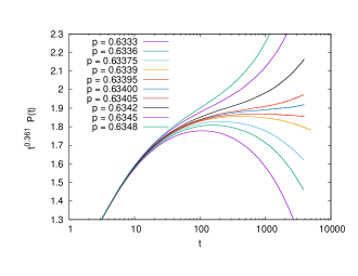
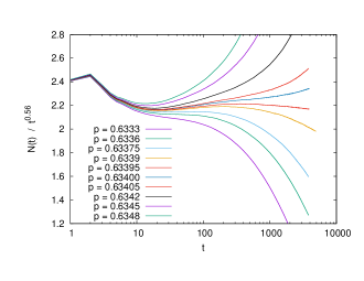
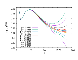
Figure 1: (color online) Top to bottom panels: Log-log plots of survival probability $P(t)$, average number of growth sites $N(t)$, and r.m.s. distance of growth sites from the seed, all plotted against time $t$. Each curve is for one fixed value of $p$, with $p$ decreasing from top to bottom. For more significance, a power of $t$ with suitable exponent is multiplied to each curve, so that the critical curves are roughly horizontal.

In a second set of runs we used lattices with helical b.c. and followed the cluster growth until it stopped because all wettable sites were already wetted, and measured properties like the cluster mass distribution $p(m)$, the dependence of the average cluster mass on $L$, and the density of the giant cluster (which is also the probability that a spreading from a single-site seed leads to a giant cluster).

Finally, in a third set of runs we used lattices of size $L\times L\times L_{z}$ with $L_{z}\gg L$. Initial conditions did not consist of single “wet” (or infected, in the interpretation of epidemic growth) points, but the entire plane $z=0$ was wet/infected, and the spreading was allowed only into the region $z>0$. Lateral boundary conditions were either periodic or open, but the b.c. at $z=L_{z}$ was not specified because it was checked that all clusters stopped growing for $z<L_{z}$. This was feasible, because these simulations were only done in the subcritical phase $p<p_{c}$. In this way we could measure spanning probabilities: On a given disorder realization and for any $z_{\rm max}\leq L_{z}$, there exists a cluster that spans from $z=0$ to $z=z_{\rm max}$, iff the growth stops at $z=z_{\rm max}$.

Results of the first (time-dependent, or “dynamical”) set of measurements are shown in Fig. 1. None of the curves in any of the three panels is really a straight line, indicating substantial corrections to scaling. In spite of this, one can identify a value $p_{c}\approx 0.63397$ where the curves in all three panels seem to become straight and horizontal for large $t$. This gives us a first rough set of exponent estimates, $\delta=0.361,\eta=0.56,$ and $z=0.765$. We have not yet given error estimates, since we have two more sources of information: The finite lattice simulations for $t\to\infty$ and, more importantly, the fan-outs of the curves in Fig. 1. The latter gives us an independent estimate of the correlation length exponent $\nu$. More precisely, we have finite-$t$ scaling laws like

$$P(t,p)=t^{-\delta}\phi[(p-p_{c})t^{1/\nu_{t}}]+\ldots,$$ (3)

and similar equations for $N$ and $R$. Here $\phi[x]$ is a scaling function that is analytic at $x=0$, and $\nu_{t}=\nu/z$.

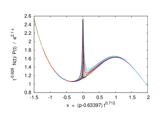
Figure 2: (color online) Plot of $t^{-0.928}N(t)/P(t)\exp(-2.1x)$ against $x=(p-p_{c})t^{1/\nu_{t}}$, where $p_{c}$ is the value estimated above, and $\nu_{t}=0.712$. The factor $\exp(-2.1x)$ was divided out in order to reduce the range on the y-axis from about three decades to half a decade. The values of $p$ used in this plot ranged from $0.623$ to $0.651$.

We checked Eq. (3) [and analogous ansatzes for the other observables] by plotting $t^{\delta}P(t,p)$ against $(p-p_{c})t^{1/\nu_{t}}$. Parameters $p_{c}$ and $\nu_{t}$ were chosen to obtain the best data collapse. In view of the strong corrections to scaling seen already in Fig. 1, we cannot indeed expect a perfect collapse, but we shall try to get a good collapse for large $t$. Results of such an attempt, this time not for $P$ but for the number $N/P$ of growth sites per still growing cluster, are shown in Fig. 2. This time we used a much wider range of $p$-values, $p\in[0.623,0.651]$. In this wide range $\phi$ would take a vast range of values, making a collapse plot look excellent but virtually useless. In order to increase significance, we have divided $\phi[x]$ by $\exp(2.1x)$. We see excellent collapse in the wings in Fig. 2, but huge deviations at $x\approx 0$ which precisely result from the small-$t$ corrections seen also in Fig. 1. Notice that we also changed slightly the exponent from the above estimate, in order to optimize the data collapse.

Having obtained in this way $\nu_{t}\approx 1.404$, we can now also estimate other exponents like $\nu=z\nu_{t}$ and $\beta=\delta\nu_{t}$.

For the second set of runs we used lattice sizes ranging from $32^{3}$ to $2048^{3}$. We do not show any results, as they were fully compatible with the dynamical simulations but proved to be less significant. In any case, we verified that the fractal dimension $D_{f}$ (governing the cutoff of the mass distribution) and the exponents $\tau$ (describing its power law decay) are obtained in perfect agreement with the scaling relations $D_{f}=3-\beta/\nu$ and $\tau=d/D_{f}+1$.

As a final result we obtain $p_{c}=0.633965(15)$ and the mutually consistent set of exponents $\delta=0.364(3),\eta=0.560(8),z=0.765(3),\nu_{t}=1.404(5),\nu=1.074(5),\beta=0.511(5),D_{f}=2.524(8),\tau=2.189(5).$ As for any critical exponent estimates, the errors here are not statistical but are mainly systematic errors due to uncertainties in the finite size corrections. Since critical exponent estimation involves an extrapolation (which by its nature is ill defined), the results are highly subjective and result from judicious plausibility considerations taking into account all measured observables. Notice in particular that least square fits would not be appropriate, and are the main source of the many wrong critical exponent estimates found in the literature. While $p_{c}$ is more precise than the value quoted in Schrenk by a factor $\approx 25$, the critical exponents are typically more precise by factors 2 to 5. But in all cases the agreement is within two standard deviations.

Let us finally discuss the spanning probabilities resulting in the subcritical phase from the third set of runs. Let us denote by $\Pi(p,r,L_{z})$ the probability that there exists a spanning cluster (from $z=0$ to $z=L_{z}$) on a lattice with aspect ratio $r=L_{z}/L$, and for given $p$-value $p$. In Schrenk it was proven mathematically that $\Pi(p,r,L_{z})$ decreases with $L_{z}$, for any fixed $r$ and for fixed $p\in[0.52974\ldots,p_{c}[$, not faster than a power. This is in striking contrast to ordinary percolation, where $\Pi(p,r,L_{z})$ decreases exponentially. A closer inspection of the proof reveals that the problem is similar to that of Griffiths phases Griffiths ; Dhar ; Moreira ; Cafiero , where frozen disorder leads to slow decay of correlations in time. Here we are not dealing with disorder frozen in time, but with disorder (the columns drilled parallel to the $z$-axis) that is frozen in $z$-direction. As a consequence we should observe correlations decreasing very slowly in the $z$-direction.

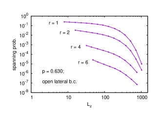
Figure 3: (color online) Log-log plot of spanning probabilities $\Pi(p=0.630,r,L_{z})$ against $L_{z}$, for fixed values of the aspect ratio $r$.

In Fig. 3 we show results for lattices with open lateral b.c. and $p=0.630$. This should be compared to Fig. 4 in Schrenk , where the same boundary conditions and the same value of $p$ were used, but which extend only to much smaller values of $L_{z}$. Due to this much smaller range of $L_{z}$, the authors of Schrenk claimed to see a power law and thus to confirm the mathematical prediction. We now see that this was not true. Although we cannot of course exclude an asymptotic power law, it should set in only at much larger values of $L_{z}$, in particular for small values of $r$. Simulations with different values of $p$ and with periodic b.c.’s, not shown here, fully confirm this.

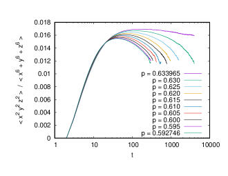
Figure 4: (color online) Log-linear plot of a moment ratio that would be equal to $1/60$ for isotropic clusters. More precisely, the data use moments of the growth site coordinates at time $t$, in clusters grown from a single point seed. Values of $p$ decrease from top to bottom.

Figure 3 suggests that presently reachable lattice sizes are not able to show the true asymptotic behavior. This is also suggested by distributions of cluster sizes and of spherical asymmetries as measured by averages of $x^{2}y^{2}z^{2}-(x^{6}+y^{6}+z^{6})/60$, of critical and sub-critical clusters grown from point seeds. They also should have power-behaved tails Schrenk . We indeed found that subcritical cluster size distributions showed some deviations from exponential decay (data not shown here), and that average asymmetries were significantly different from zero (see Fig. 4). But both were much smaller than what one would expect if the distributions were decaying like powers. Thus we conclude that the above results for the critical exponents might also not yet represent the true asymptotic behavior – which should be visible only for cluster and lattice sizes not reachable with present computational means. The total amount of CPU time (on PC’s and laptops) spent on this project was about a year.

In summary, we have verified that drilling percolation is in a new universality class, different from ordinary (Bernoulli) percolation, but the true asymptotic behavior might be still different from what is seen in Schrenk and in the present simulations. Let us finally discuss some possible generalizations.

The most obvious generalization is mixed drilling / Bernoulli percolation, where we take out both single sites and columns. We conjecture that in this case the long range aspect of the columns is relevant, and the model should be in the universality class of drilling percolation.

Next, we can consider the case where linear objects are again taken out, but they are oriented randomly, without any reference to coordinate axes Hilario . This seems to be more delicate. It is plausible that it is not in the universality class of ordinary percolation, but it might be in a universality class of its own. The same might be true for the case that there is a finite number $>3$ of possible orientations, e.g. coordinate axes and space diagonals. While the present algorithm would not work for completely random orientations, it could still be generalized to include diagonals.

More interesting from a theoretical point of view are higher dimensions, $d\geq 4$. For space dimension $d$ we can “drill” out subspaces of dimensions $\leq d-2$ and still have a non-trivial connectedness problem. For $d=4$, e. g., taking out columns and planes would still give non-trivial percolation problems. We conjecture that these are in different universality classes. As one goes to higher and higher dimensions, one expects then a proliferation of universality classes. It seems however non-trivial to check this by simulations, and it is not clear how to treat them analytically.

Finally, we shall study in a forthcoming paper Grass2017 a 3-d model with columnar defects in one direction only and with additional point (Bernoulli) defects. This model shows a much clearer Griffiths phase, and much stronger anisotropies even at the critical point.

I thank the authors of Schrenk , in particular K.J. Schrenk, M. Hilario, and V. Sidoravicius, for stimulating correspondence. I also thank N. Araújo for carefully reading the manuscript.

References

- (1) N. Araújo, P. Grassberger, B. Kahng, K. J. Schrenk, and R. M. Ziff, The European Physical Journal Special Topics 223, 2307 (2014).
- (2) K.J. Schrenk et al., Phys. Rev. Lett. 116, 055701 (2016).
- (3) Y. Kantor, Phys. Rev. B 33 , 3522 (1986).
- (4) D. J. Amit, Field Theory, the Renormalization Group and Critical Phenomena, 2nd Ed. (World Scientific Press, 1984).
- (5) A. Weinrib, Phys. Rev. B 29, 387 (1984).
- (6) P. L. Leath, Phys. Rev. B 14, 5046 (1976).
- (7) T.H. Cormen, C.E. Leiserson, R.L. Rivest, and C. Stein, Introduction to Algorithms, 2nd ed. (MIT Press and McGraw-Hill, 2001).
- (8) R.B. Griffiths, Phys. Rev. Lett. 23, 17 (1969).
- (9) D. Dhar, M. Randeria, and J.P. Sethna, Europhys. Lett. 5, 485 (1988).
- (10) A.G. Moreira and R. Dickman, Phys. Rev. E 54, R3090 (1996).
- (11) R. Cafiero, A. Gabrielli, and M.A. Muñoz, Phys. Rev. E 57, 5060 (1998).
- (12) M.R. Hilário, V. Sidoravicius, and A. Teixeira, Prob. Theory Relat. Fields 163, 613 (2015).
- (13) P. Grassberger, to be published.