Effective potential for relativistic scattering

We consider quantum inverse scattering with singular potentials and calculate the Sine-Gordon model effective potential in the laboratory and centre-of-mass frames. The effective potentials are frame dependent but closely resemble the zero-momentum potential of the equivalent Ruijsenaars-Schneider model.

1 Introduction and motivation

In recent years advances in lattice QCD techniques made possible to measure and study forces between nucleons. A major success was the first principles calculation of the two-nucleon potential by the HAL QCD collaboration [1, 2, 3], which was later extended to nucleon-hyperon interactions [4, 5] and to the study of three-baryon forces [6]. Three-neutron (and higher) interactions are crucial to determine the correct nuclear equation of state, which is used in the calculation of the mass and radius of neutron stars. Gravitational wave signals expected from inspiraling neutron star systems are sensitive to the resulting mass-radius relation.

The HAL QCD method [1] is based on measuring the Nambu-Bethe-Salpeter (NBS) wave function $\Psi_{E}({\mathbf{x}})$ of a two-nucleon state which satisfies (in the centre of mass frame) the “Schrödinger equation”

$$\left[-\frac{1}{m}\nabla^{2}+U_{E}({\mathbf{x}})\right]\Psi_{E}({\mathbf{x}})=E\,\Psi_{E}({\mathbf{x}}),$$ (1)

where $m$ is the nucleon mass. Due to the relativistic nature of the problem, the NBS “potential” $U_{E}({\mathbf{x}})$ is energy-dependent. This energy-dependence however is found to be weak and the NBS potential at low energies resembles the phenomenological nuclear potential used in nuclear physics for many decades [7, 8, 9]. In particular, at short distances it has a characteristic repulsive core.

The problem of energy dependence can be studied in some $1+1$ dimensional integrable models [10]. The Ising model and the O$(3)$ nonlinear $\sigma$-model were studied and it was found that at low energies the energy-dependent $U_{E}({\mathbf{x}})$ can be well approximated by its zero-momentum limit (corresponding to the case where the relative momentum of the two-particle state vanishes). The problem was also studied in the Sine-Gordon (SG) model [11]. In the semiclassical limit an energy-independent effective potential was constructed, which exactly reproduces the semiclassical time delays for all energies. This could be compared to the zero-momentum potential, which is explicitly known in this model from its equivalent Ruijsenaars-Schneider (RS) formulation [12, 13].

In this paper we continue to study the notion of effective potential in the integrable (analytically solvable) SG model in $1+1$ dimension. We model the way the phenomenological potential was determined from scattering experiments: we require that the quantum mechanical effective potential exactly reproduces the (analytically known) scattering phase shifts at all energies. The price we have to pay is that the effective potential is frame dependent. We will construct the effective potential in the laboratory frame of the scattering process and also in the centre of mass frame of the two particles. We will compare them to each other and to the zero-momentum potential known from the RS formulation of the model.

The paper is organized as follows. In section 2 we define the notion of effective potential for relativistic scattering. Section 3 is a review of quantum mechanical inverse scattering in one dimension. We generalize known results for the case of singular potentials. In section 4 and 5 we calculate the effective potential for soliton-soliton scattering in the SG model in the laboratory and centre-of-mass frames, respectively. Section 6 is a short summary of the results and contains our conclusions. Some technical details and examples can be found in the appendices together with the summary of the scattering phase shifts in the SG model.

2 Effective potentials

We will study the one-dimensional scattering of two identical partices of mass $m$ (with positions $x_{1}$, $x_{2}$ and momenta $p_{1}$, $p_{2}$), whose interaction has a strong repulsive core which does not allow the particles to come close to each other. If initially particle 1 is to the left of particle 2 then $x_{2}>x_{1}$ at all times. Initially $p_{1}>p_{2}$:

$\bullet$ $\longrightarrow$ $p_{1}$                                                      $p_{2}$ $\longleftarrow$ $\bullet$

$x_{1}$                                                                            $x_{2}$

Asymptotically, for $(x_{2}-x_{1})\to\infty$, the 2-particle wave function $\Phi(x_{1},x_{2})$ is a superposition of free waves:

$$\Phi(x_{1},x_{2})\approx\Phi_{\rm as}(x_{1},x_{2})={\rm e}^{i(k_{1}x_{1}+k_{2}x_{2})}+S(p_{1},p_{2}){\rm e}^{i(k_{2}x_{1}+k_{1}x_{2})},\qquad\quad x_{2}-x_{1}>>0.$$ (2)

Here the first term is the incoming free wave and the second one is the outgoing free wave which has picked up the phase factor $S(p_{1},p_{2})$ as a result of the interaction. We have introduced the wave vectors $k_{j}=p_{j}/\hbar$, $j=1,2$.

For relativistic scattering, the “S-matrix” $S(p_{1},p_{2})$ is a function of the relative rapidity of the particles:

$$S_{\rm R}(p_{1},p_{2})=-\Sigma(\theta_{1}-\theta_{2}),\qquad\qquad p_{j}=mc\sinh\theta_{j}.$$ (3)

For non-relativistic scattering we can use a quantum-mechanical description with a potential depending on the relative distance of the particles. The Hamilton operator has the form

$$\hat{\cal H}=-\frac{\hbar^{2}}{2m}\,\frac{\partial^{2}}{\partial x_{1}^{2}}-\frac{\hbar^{2}}{2m}\,\frac{\partial^{2}}{\partial x_{2}^{2}}+U(x_{2}-x_{1}).$$ (4)

We have to find a solution of the Schrödinger equation

$$\hat{\cal H}\Phi=E\Phi,\qquad\qquad E=\frac{\hbar^{2}}{2m}(k_{1}^{2}+k_{2}^{2})$$ (5)

with asymptotics (2). Separating the centre of mass and relative motions we can write

$$\Phi(x_{1},x_{2})={\rm e}^{iK(x_{1}+x_{2})}\Psi(x_{2}-x_{1}),$$ (6)

where the relative wave function satisfies the Schrödinger equation

$$-\frac{\hbar^{2}}{m}\Psi^{\prime\prime}(x)+U(x)\Psi(x)=\frac{\hbar^{2}}{m}\kappa^{2}\Psi(x).$$ (7)

Here

$$k_{1}=K+\kappa,\quad k_{2}=K-\kappa,\qquad\quad E=\frac{\hbar^{2}}{m}(K^{2}+\kappa^{2}),\qquad\kappa>0.$$ (8)

The $x\to\infty$ asymptotics of the relative wave function is required to be of the form

$$\Psi(x)\approx\Psi_{\rm as}(x)=-{\cal T}(\kappa){\rm e}^{i\kappa x}+{\rm e}^{-i\kappa x},\qquad x>>0.$$ (9)

Comparing to (2) gives

$$S_{\rm NR}(p_{1},p_{2})=-{\cal T}\left(\frac{p_{1}-p_{2}}{2\hbar}\right).$$ (10)

We can simplify the problem by introducing a length scale $\ell$ and rescaling the variables. We introduce

$$u(x)=\Psi(\ell x),$$ (11)

which satisfies

$$-u^{\prime\prime}(x)+q(x)u(x)=k^{2}u(x)$$ (12)

with

$$q(x)=\frac{m\ell^{2}}{\hbar^{2}}U(\ell x),\qquad\quad k=\ell\kappa$$ (13)

and has asymptotics

$$u_{\rm as}(x)={\rm e}^{-ikx}-S(k){\rm e}^{ikx},\qquad\quad{\cal T}(\kappa)=S(\kappa\ell).$$ (14)

The length scale is arbitrary but it is convenient to choose $\ell=2L$, where $L$ is the Compton wavelength of the particle, $L=\hbar/mc$. With this choice

$$S_{\rm NR}(p_{1},p_{2})=-S\left(\frac{p_{1}-p_{2}}{mc}\right),\qquad\quad U(x)=\frac{mc^{2}}{4}q\left(\frac{x}{2L}\right).$$ (15)

Our aim is to find a suitable effective potential $U(x)$ that, by solving the corresponding nonrelativistic Schrödinger equation, leads to the physical, i.e. relativistic, scattering S-matrix as function of the momentum of the particles. Thus we require

$$S\left(\frac{p_{1}-p_{2}}{mc}\right)\sim\Sigma\left({\rm arcsinh}\,\left(\frac{p_{1}}{mc}\right)-{\rm arcsinh}\,\left(\frac{p_{2}}{mc}\right)\right).$$ (16)

Clearly, it is impossible to find such an effective potential in general, since the true (relativistic) S-matrix is a function of the rapidity difference, whereas the non-relativistic formula depends on the momentum difference. The identification is possible only approximately at low energies, where $p_{j}\approx mc\theta_{j}$.

There are, however, two important special cases, where exact identification is possible. In the laboratory (fixed target) frame of the scattering we can require

$$({\rm LAB})\ \ \qquad S_{I}(k)=\Sigma\big{(}{\rm arcsinh}\,(k)\big{)},\qquad\quad p_{1}=kmc,\quad p_{2}=0.$$ (17)

Similarly, in the centre of mass frame we require

$$({\rm COM})\qquad S_{II}(k)=\Sigma\big{(}2\,{\rm arcsinh}\,(k/2)\big{)},\qquad p_{1}=-p_{2}=kmc/2.$$ (18)

The resulting effective potentials $U_{I}(x)$ and $U_{II}(x)$ will be different. The price we have to pay is frame dependence.

The problem we have to solve in both cases is to find the potential $q(x)$ in (12) if the corresponding S-matrix $S(k)$ is given. We are interested in potentials with a strong repulsive core, which means that $q(x)$ has to be singular when the relative distance $x$ approaches zero. This leads us to the mathematical problem of quantum inverse scattering with singular potentials, which is discussed in the next section.

3 Quantum inverse scattering with singular potentials

Quantum inverse scattering, the problem of finding the potential from scattering data, is a classical problem in quantum mechanics. It has been completely solved in the one-dimensional case [14, 15, 16] both for the entire line and the half line cases. The latter case is more important because the same mathematical problem emerges for three-dimensional spherically symmetric potentials after partial wave expansion. Here we will also be interested in this case, because we consider strongly repulsive potentials. The details of the reconstruction procedure depend on the class of the potentials and the simplest case is that of regular potentials [17]. We will proceed along the lines presented in [17], with some modifications necessary due to the singular core of our potentials.

We will consider the Schrödinger equation on the half line $x\geq 0$

$$-u^{\prime\prime}(x)+q(x)u(x)=k^{2}u(x)$$ (19)

with boundary condition $u(0)=0$. We will assume that the potential $q(x)$ is singular as $x\to 0$, more precisely we assume

$$q(x)\sim\frac{p(p-1)}{x^{2}},\qquad\quad x\to 0,$$ (20)

where $p>1$. (Later we will see that we recover the results for regular potentials in the limit $p\to 1$.) We also assume that

$$q(x)\to 0\qquad\quad{\rm as}\qquad\quad x\to\infty,$$ (21)

and that it vanishes faster than $1/x^{2}$.

3.1 Direct scattering

For any given $k$, we will need three special solutions of the differential equation (19). The physical solution $\varphi(x,k)$ is defined by its regular behaviour near the origin,

$$\varphi(x,k)=x^{p}[1+{\rm O}(x)],\qquad\quad x\to 0.$$ (22)

The singular solution $\tilde{\varphi}(x,k)$ is defined by the requirement

$$\tilde{\varphi}(x,k)=x^{1-p}[1+{\rm O}(x)],\qquad\quad x\to 0.$$ (23)

Finally the Jost solution is defined to have large $x$ asymptotics

$$f(x,k)={\rm e}^{ikx}[1+{\rm O}(1/x)],\qquad\quad x\to\infty.$$ (24)

In addition to the scattering solutions with real momentum $k$, the Schrödinger equation (19) may have normalizable bound state solutions with imaginary $k$ (negative energy). Since in our main example in this paper (soliton-soliton interaction in the Sine-Gordon model) there are no bound states we will discuss here the case without bound states. It is easy to work out the modifications necessary for potentials with bound states.

Since the second order differential equation (19) has only two linearly independent solutions, any of the above solutions can be expressed as linear combinations of the other two. For example, the Jost solution can be written as

$$f(x,k)=\tilde{f}(k)\varphi(x,k)+f(k)\tilde{\varphi}(x,k)$$ (25)

with some coefficients $\tilde{f}(k)$, $f(k)$. $f(k)$ is called the Jost function and plays an important role in scattering theory. It can be shown that $f(k)$ can alternatively be defined by the linear combination

$$\varphi(x,k)=\frac{2p-1}{2ik}\left\{f(-k)f(x,k)-f(k)f(x,-k)\right\}.$$ (26)

For real $k$

$$f^{*}(x,k)=f(x,-k)\qquad\qquad{\rm and}\qquad\qquad f^{*}(k)=f(-k)$$ (27)

and if we introduce the modulus and phase of $f(k)$ by writing

$$f(k)=|f(k)|{\rm e}^{-i\delta(k)}$$ (28)

we see that

$$|f(k)|=|f(-k)|\qquad{\rm and}\qquad\delta(-k)=-\delta(k)\quad{\rm mod\ }2\pi.$$ (29)

From (26) we see that for large $x$ asymptotically

$$\varphi(x,k)\approx-\frac{2p-1}{2ik}f(k)\left\{{\rm e}^{-ikx}-S(k){\rm e}^{ikx}\right\}=\frac{2p-1}{k}|f(k)|\sin[kx+\delta(k)].$$ (30)

Here

$$S(k)=\frac{f(-k)}{f(k)}={\rm e}^{2i\delta(k)}$$ (31)

and $\delta(k)$ is the phase shift.

It is possible to show that the large $k$ behaviour of the Jost function is

$$f(k)\approx\frac{\Gamma(2p-1)}{\Gamma(p)}(-2ik)^{1-p}[1+{\rm O}(1/k)].$$ (32)

This gives

$$\delta(k)=\frac{\pi}{2}(1-p)+{\rm O}(1/k),\qquad\quad\delta(\infty)=\frac{\pi}{2}(1-p).$$ (33)

Since (mod $2\pi$) $\delta(-\infty)=-\delta(\infty)$, $S(\infty)$ and $S(-\infty)$ are not the same in general, except for integer $p$, in which case

$$S(\infty)=S(-\infty)=(-1)^{p-1}.$$ (34)

The physical solutions $\varphi(x,k)$ satisfy the completeness relation

$$\frac{2}{\pi}\int_{0}^{\infty}\frac{k^{2}{\rm d}k}{(2p-1)^{2}|f(k)|^{2}}\varphi(x,k)\varphi(y,k)=\delta(x-y).$$ (35)

An other important object in inverse scattering theory is the transformation kernel $A(x,y)$. It is defined as the unique solution of the Goursat problem

$$\frac{\partial^{2}}{\partial x^{2}}A(x,y)=\frac{\partial^{2}}{\partial y^{2}}A(x,y)+q(x)A(x,y),$$ (36)

$$-2\frac{{\rm d}}{{\rm d}x}A(x,x)=q(x),$$ (37)

$$\lim_{(x+y)\to\infty}A(x,y)=\lim_{(x+y)\to\infty}\frac{\partial}{\partial x}A(x,y)=\lim_{(x+y)\to\infty}\frac{\partial}{\partial y}A(x,y)=0.$$ (38)

This transformation kernel can be used to define the unitary operator $\hat{\cal A}$ which maps the solutions of the free problem onto those of the interacting problem with potential $q(x)$. The action of $\hat{\cal A}$ is defined by

$$\big{(}\hat{\cal A}{\cal F}\big{)}(x)={\cal F}(x)+\int_{x}^{\infty}{\rm d}yA(x,y){\cal F}(y)$$ (39)

and the mapping is

$$f_{k}=\hat{\cal A}E_{k},\qquad\qquad f_{k}(x)=f(x,k),\qquad E_{k}(x)={\rm e}^{ikx}.$$ (40)

3.2 Inverse scattering

Starting from the completeness relation (35), by acting on it with the inverse of the unitary operator $\hat{\cal A}$, one can derive the most important equation of inverse scattering, the Marchenko integral equation. We have followed the steps presented in [17] for regular potentials. In our case with singular potential one has to be careful because unlike for regular potentials, $\delta(\infty)\not=0$ here. The result is that $A(x,y)$ satisfies the Marchenko equation

$$F(x+y)+A(x,y)+\int_{x}^{\infty}{\rm d}s\,A(x,s)\,F(s+y)=0,\qquad\quad y>x>0,$$ (41)

where

$$F(x)=\frac{1}{2\pi ix}\int_{-\infty}^{\infty}{\rm d}k{\rm e}^{ikx}S^{\prime}(k).$$ (42)

The Marchenko equation (41) is of the same form as for regular potentials, only the definition of $F(x)$ had to be modified. In the special case of integer $p$, an alternative form of (42) is obtained by partial integration

$$F(x)=\frac{1}{2\pi}\int_{-\infty}^{\infty}{\rm d}k{\rm e}^{ikx}\left[(-1)^{p-1}-S(k)\right].$$ (43)

For $p=1$ the standard formula [17] is reproduced.

Quantum inverse scattering now proceeds in three steps. The first step is to calculate $F(x)$ using the scattering data $S(k)$ in (42) or (43). The second step is to solve (41) for $A(x,y)$. The third and final step is to use

$$-2\frac{{\rm d}}{{\rm d}x}A(x,x)=q(x)$$ (44)

to determine $q(x)$.

4 Sine-Gordon effective potential in the laboratory frame

In this section we carry out the three steps of quantum inverse scattering to determine the effective SG potential that exactly reproduces the SG soliton-soliton scattering in the laboratory frame (case I). The SG S-matrix is given in Appendix B.

For simplicity, we deal with integer $p$ only. Using the identification (17) and the SG S-matrix (95) we have

$$S_{I}(k)=\prod_{m=1}^{p-1}\frac{s_{m}-ik}{s_{m}+ik},\qquad\quad s_{m}=\sin(\nu\pi m).$$ (45)

The first step is to calculate $F(x)$. For the above S-matrix (43) is easily evaluated with the help of the residue theorem and we obtain

$$F(x)=-\sum_{m=1}^{p-1}R_{m}\,{\rm e}^{-s_{m}x},\qquad\qquad R_{m}=2s_{m}\prod_{n\not=m}\frac{s_{n}+s_{m}}{s_{n}-s_{m}}.$$ (46)

The next step is to solve the Marchenko equation for $A(x,y)$. For $F(x)$ given by (46) we have to solve

$$-\sum_{m}R_{m}{\rm e}^{-s_{m}(x+y)}+A(x,y)-\sum_{m}R_{m}{\rm e}^{-s_{m}y}\int_{x}^{\infty}{\rm d}w\,A(x,w){\rm e}^{-s_{m}w}=0.$$ (47)

We see that the $y$ dependence of $A(x,y)$ must be of the form

$$A(x,y)=\sum_{m}R_{m}a_{m}(x){\rm e}^{-s_{m}y}.$$ (48)

When this expression is substituted back to (47) we find

$$a_{m}(x)={\rm e}^{-s_{m}x}+\sum_{n}R_{n}\int_{x}^{\infty}{\rm d}w\,a_{n}(x){\rm e}^{-(s_{m}+s_{n})w}.$$ (49)

The $w$ integration can be performed and we get

$$a_{m}(x)={\rm e}^{-s_{m}x}+\sum_{n}R_{n}\,a_{n}(x)\frac{1}{s_{m}+s_{n}}{\rm e}^{-(s_{m}+s_{n})x},$$ (50)

which can be further simplified by introducing

$$a_{m}(x)={\rm e}^{-s_{m}x}\,b_{m}(x),\qquad\qquad z_{m}(x)=R_{m}\,{\rm e}^{-2s_{m}x}.$$ (51)

We finally obtain the equations

$$b_{m}=1+\sum_{n}\frac{z_{n}\,b_{n}}{s_{m}+s_{n}}.$$ (52)

This way the Marchenko integral equation is reduced to an algebraic problem. We have to solve (52) for the $b_{m}$ variables and using this solution we can write

$$A(x,y)=\sum_{m}R_{m}\,b_{m}(x)\,{\rm e}^{-s_{m}(x+y)}.$$ (53)

Finally $A(x,x)$ is given by

$$A(x,x)=\sum_{m}b_{m}(x)\,z_{m}(x).$$ (54)

Figure 1: Comparison of the integrated effective potential $A(x,x)$ (solid) and the corresponding zero-momentum $A_{o}(x,x)$ (dashed) for $p=3$.

The solution of this algebraic problem turns out to be very simple. We can rearrange (52) to the matrix form

$$\sum_{n}{\cal M}_{mn}\,b_{n}=1$$ (55)

where

$${\cal M}_{mn}(x)=\delta_{mn}-\frac{z_{n}(x)}{s_{m}+s_{n}}.$$ (56)

As shown in Appendix C, the solution is the logarithmic derivative of the determinant of this matrix,

$$A(x,x)=\frac{{\rm d}}{{\rm d}x}\ln{\cal D}(x),\qquad\qquad{\cal D}(x)={\rm Det}\,\left({\cal M}(x)\right).$$ (57)

The final results can be further simplified if we introduce the “reduced” determinant $\hat{\cal D}$ by writing

$${\cal D}=2^{p-1}\,\left(\prod_{k<l}\frac{1}{s_{k}-s_{l}}\right)\left(\prod_{m}{\rm e}^{-s_{m}x}\right)\hat{\cal D}.$$ (58)

Since the determinant is a totally symmetric expression of the variables $s_{j}$ and the prefactor is totally antisymmetric, the reduced determinant must also be totally antisymmetric. Moreover, it turns out to be a polynomial in the variables $s_{j}$, $H_{j}$, $C_{j}$, where

$$H_{j}=\sinh(s_{j}x),\qquad\qquad C_{j}=s_{j}\cosh(s_{j}x).$$ (59)

It is easy to see that for $p=2$ we have $\hat{\cal D}=H_{1}$. We have calculated the reduced determinant for $p=3,4,5$ using Mathematica. For $p=3$

$$\hat{\cal D}=C_{1}H_{2}-C_{2}H_{1},$$ (60)

for $p=4$

$$\hat{\cal D}=-(s_{1}^{2}-s_{2}^{2})C_{3}H_{1}H_{2}+(s_{1}^{2}-s_{3}^{2})C_{2}H_{1}H_{3}-(s_{2}^{2}-s_{3}^{2})C_{1}H_{2}H_{3},$$ (61)

finally for $p=5$ Mathematica found

$$\hat{\cal D}=-(s_{1}^{2}-s_{2}^{2})(s_{3}^{2}-s_{4}^{2})C_{1}C_{2}H_{3}H_{4}\quad+\quad{\rm 5\ anti-permutations}.$$ (62)

The 5 additional terms on the right hand side of (62) make it totally antisymmetric.

From the above formulas it is clear how $\hat{\cal D}$ can be constructed from the variables $s_{j}$, $H_{j}$, $C_{j}$ in general. Since our calculation is algebraic, it must be valid also for the case discussed in Appendix A, since the corresponding S-matrix is also of the form (45), with $s_{m}=m$. It is a very non-trivial check on our result that in this case (57) is reduced to

$$\frac{p(p-1)}{2}[\coth(x)-1],$$ (63)

which is by far not obvious, but turns out to be true.

The small $x$ expansion of (57) takes the form

$$\begin{split}A(x,x)&=\frac{p(p-1)}{2x}-\sum_{j}s_{j}+\frac{x}{2p-1}\left(\sum_{j}s_{j}^{2}\right)+{\rm O}(x^{3})\\ &=\frac{p(p-1)}{2x}-\frac{1}{2}\cot\frac{\pi\nu}{2}+\frac{x}{4}+{\rm O}(x^{3}).\end{split}$$ (64)

The strength of the $x\to 0$ singularity is exactly the same as we assumed at the beginning of our considerations.

We have compared the (integrated) laboratory frame effective potential and the (integrated) zero-momentum potential in Figs. 1,2 for $p=3,4$.

Figure 2: Comparison of the integrated effective potential $A(x,x)$ (solid) and the corresponding zero-momentum $A_{o}(x,x)$ (dashed) for $p=4$.

5 Sine-Gordon effective potential in the centre of mass frame

In this section we calculate the SG effective potential in the centre of mass frame. Again, we restrict our attention to integer $p$. Using (18) and (95) we have

$$S_{II}(k)=\prod_{m=1}^{p-1}\frac{s_{m}-ik\rho(k)}{s_{m}+ik\rho(k)},\qquad\quad\rho(k)=\sqrt{1+\frac{k^{2}}{4}}.$$ (65)

This can be equivalently written

$$S_{II}(k)=(-1)^{p-1}+\sum_{m}\frac{R_{m}}{s_{m}+ik\rho(k)}$$ (66)

and correspondingly, using (43),

$$F_{II}(x)=-\sum_{m}R_{m}{\cal F}(x;s_{m}),$$ (67)

where

$${\cal F}(x;\sigma)=\frac{1}{2\pi}\int_{-\infty}^{\infty}{\rm d}k\,\frac{{\rm e}^{ikx}}{\sigma+ik\rho(k)}.$$ (68)

Let us introduce the notations

$$\sigma=\sin\varphi,\qquad\tilde{\sigma}=\cos\varphi,\qquad\qquad\alpha=\sin\frac{\varphi}{2},\qquad\beta=\cos\frac{\varphi}{2}.$$ (69)

The integrand of (68) in the upper half plane has poles at $k=2i\alpha$, $2i\beta$ with residues $-i\beta/\tilde{\sigma}$, $i\alpha/\tilde{\sigma}$ respectively and a cut starting at $k=2i$ and going up along the imaginary axis. We can evaluate the Fourier integral by closing the contour with a half-circle at infinity and using the residue theorem, but we have to add the contribution of the cut as well. The contribution of the poles is

$${\cal F}^{{\rm pole}}(x;\sigma)=\frac{1}{\tilde{\sigma}}\left(\beta{\rm e}^{-2\alpha x}-\alpha{\rm e}^{-2\beta x}\right)$$ (70)

and we can write

$${\cal F}(x;\sigma)={\cal F}^{{\rm pole}}(x;\sigma)+{\cal F}^{{\rm cut}}(x;\sigma),$$ (71)

where

$${\cal F}^{{\rm cut}}(x;\sigma)=-\frac{1}{\pi}\int_{2}^{\infty}{\rm d}\kappa\,\frac{\kappa R{\rm e}^{-\kappa x}}{\sigma^{2}+\kappa^{2}R^{2}},\qquad\quad R=\sqrt{\frac{\kappa^{2}}{4}-1}.$$ (72)

This form is more suitable for numerical evaluation because instead of an oscillating integrand it contains a decaying exponential.

Figure 3: The integrated effective potential in the COM frame for $p=2$ (dots). For comparison the analytically obtained LAB frame integrated effective potential $A(x,x)$ (solid) is also shown.

We calculated $F_{II}(x)$ numerically for $p=2$, $3$ and by discretizing the integrals solved the corresponding Marchenko equations numerically. The results are shown in Figs. 3,4. For comparison we also show in these plots the corresponding LAB frame (integrated) effective potentials. It can be seen that the frame dependence is weak: both effective potentials have the same qualitative features and are close to each other. The expected $1/x$ short distance behaviour is also reproduced. We can conclude that the notion of effective potential makes sense in this model.

Figure 4: The integrated effective potential in the COM frame for $p=3$ (dots). For comparison the analytically obtained LAB frame integrated effective potential $A(x,x)$ (solid) is also shown.

6 Summary and conclusion

The phenomenological potential in nuclear phsysics has a limited range of applicability because the very notion of a potential used in the Schrödinger equation is a nonrelativistic concept which is meaningful and valid (approximately) only below the $\pi$-production threshold. The NBS potential as measured by the original HAL QCD method [1] is energy dependent (although this energy dependence is moderate at low energies). An alternative possibility is to define [2, 3] an energy-independent, but nonlocal “potential”.

$1+1$ dimensional integrable models are useful because the analogous problems can be studied more explicitly. Moreover, since there is no particle production in integrable models, the two-particle description remains valid at all energies. It is possible to define an effective potential, which is energy independent and reproduces the scattering data exactly. The price one has to pay for energy independence is that due to the relativistic nature of the problem this effective potential becomes frame dependent.

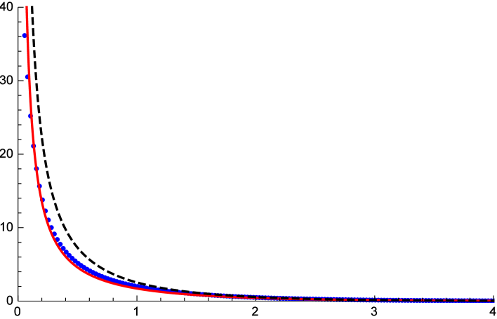
Figure 5: Comparison of integrated SG effective potentials for $p=3$. The solid (red) line, the (blue) dots and the dashed (black) line are the LAB frame, the COM frame and the zero-momentum potential, respectively.

In this paper we studied the effective potential in the SG model. We calculated the effective potential algebraically in the laboratory frame and numerically in the centre of mass frame using inverse scattering techniques. Our results are summarized in Fig. 5, where the LAB and COM frame effective potentials are compared and the zero-momentum potential (obtained from the equivalent Ruijsenaars-Schneider formulation of the model) is also shown. The three potentials are qualitatively very similar and also close numerically. Our conclusion is that (at least in this $1+1$ dimensional toy model) in spite of the problems discussed above the effective potential remains a useful concept.

Acknowledgments

This work was supported by the Major State Basic Research Development Program in China (No. 2015CB856903), the National Natural Science Foundation of China (Grant No. 11575254) and by the Hungarian National Science Fund OTKA (under K116505). J. B. would like to thank the CAS Institute of Modern Physics, Lanzhou, where most of this work has been carried out, for hospitality.

Appendix A Scattering and inverse scattering for the $1/\sinh^{2}x$ potential

To illustrate the steps of direct and inverse scattering, we take the solvable potential

$$q(x)=\frac{p(p-1)}{\sinh^{2}x}.$$ (73)

The solution of the Schrödinger equation (19) with this potential is well known and proceeds by introducing the new variables

$$u(x)={\rm e}^{ikx}F(z),\qquad\qquad z=\frac{1}{2}(1+\coth x).$$ (74)

The Schrödinger equation becomes

$$z(1-z)F^{\prime\prime}(z)+(1+ik-2z)F^{\prime}(z)+p(p-1)F(z)=0,$$ (75)

which is the hypergeometric differential equation with parameters

$$a=p,\qquad\quad b=1-p,\qquad\quad c=1+ik.$$ (76)

The hypergeometric differential equation has many solutions expressible by Gauss’ hypergeometric function ${}_{2}F_{1}$. The solutions we need are

$$\varphi(x,k)=\frac{1}{2^{p}}\left(1-{\rm e}^{-2x}\right)^{p}{\rm e}^{ikx}{}_{2}F_{1}\left(p,p-ik,2p;1-{\rm e}^{-2x}\right),$$ (77)

$$\tilde{\varphi}(x,k)=2^{p-1}\left(1-{\rm e}^{-2x}\right)^{1-p}{\rm e}^{ikx}{}_{2}F_{1}\left(1-p-ik,1-p,2-2p;1-{\rm e}^{-2x}\right),$$ (78)

$$f(x,k)=\left(1-{\rm e}^{-2x}\right)^{p}{\rm e}^{ikx}{}_{2}F_{1}\left(p,p-ik,1-ik;{\rm e}^{-2x}\right).$$ (79)

$\varphi(x,k)$ and $f(x,k)$ are always well defined by the above formula, but the above expression for $\tilde{\varphi}(x,k)$ is valid only if $p$ is not an integer or half-integer. This is a technical difficulty only and does not imply that $\tilde{\varphi}(x,k)$ does not exist in these cases. It only means that it cannot be simply expressed in terms of ${}_{2}F_{1}$. Moreover, our formulas for $f(k)$ and the S-matrix are continuous and turn out to be valid for integer/half-integer $p$ as well.

Using the well-known linear relations between the hypergeometric functions of argument $z$ and argument $1-z$ we can read off the coefficients defined by (25). In this example they turn out to be

$$f(k)=\frac{1}{2^{p-1}}\,\frac{\Gamma(1-ik)\Gamma(2p-1)}{\Gamma(p)\Gamma(p-ik)},$$ (80)

$$\tilde{f}(k)=2^{p}\,\frac{\Gamma(1-ik)\Gamma(1-2p)}{\Gamma(1-p-ik)\Gamma(1-p)}.$$ (81)

It can be checked that using (26) leads to the same expression for $f(k)$.

The S-matrix is

$$S(k)=\frac{\Gamma(1+ik)\Gamma(p-ik)}{\Gamma(1-ik)\Gamma(p+ik)}.$$ (82)

As mentioned before, this derivation is not valid for integer $p$. Nevertheless, the formula for the S-matrix remains valid for integer $p$ too. Moreover, for integer $p$ it simplifies to

$$S(k)=\prod_{j=1}^{p-1}\frac{j-ik}{j+ik}.$$ (83)

The simplest nontrivial case is $p=2$. The corresponding S-matrix is

$$S(k)=\frac{1-ik}{1+ik}$$ (84)

and (43) gives

$$F(x)=-2{\rm e}^{-x}.$$ (85)

For this $F(x)$ the Marchenko equation is easily solved and one finds

$$A(x,y)=\frac{{\rm e}^{-y}}{\sinh x}.$$ (86)

Thus

$$A(x,x)=\coth x-1$$ (87)

and using (44) the potential (73) is reproduced, as it should.

Appendix B The Sine-Gordon S-matrix

The Sine-Gordon (SG) model is perhaps the most studied two-dimensional integrable field theory. Its spectrum and S-matrix is exactly known from its bootstrap solution [18]. Moreover, an equivalent relativistic quantum mechanical description exists, the Ruijsenaars-Schneider model [12, 13].

The SG field theory Lagrangian is

$${\cal L}=\frac{1}{2}\left(\dot{\phi}^{2}-\phi^{\prime 2}\right)+\frac{\mu^{2}}{\beta^{2}}\cos(\beta\phi),$$ (88)

where $\mu$ is a mass parameter and $\beta$ is the SG coupling. The model is well-defined only if $0<\beta^{2}<8\pi$. $\beta^{2}=4\pi$ is the free fermion point. We will use the parameters

$$p=\frac{4\pi}{\beta^{2}}>\frac{1}{2}\qquad\qquad{\rm and}\qquad\qquad\nu=\frac{1}{2p-1}.$$ (89)

The spectrum of the model includes a U$(1)$ doublet of particles (soliton and antisoliton of mass $m$). There are also soliton-antisoliton bound states (breathers), whose mass spectrum is given by

$$m_{k}=2m\sin\left(\frac{\pi\nu k}{2}\right),\qquad\quad k=1,2,\dots<2p-1.$$ (90)

The soliton mass is related to the Lagrangian mass parameter by

$$m=\frac{2p-1}{\pi}\mu.$$ (91)

The full S-matrix of the model (scattering among solitons, antisolitons, breathers) is completely known [18], but in this paper we only need the soliton-soliton scattering S-matrix. Here there are no bound states and it is given by the formula

$$\Sigma(\theta)=\exp\left\{i\int_{0}^{\infty}\frac{{\rm d}\omega}{\omega}\sin\left(\frac{2\theta\omega}{\pi}\right)\frac{\sinh\big{(}(\nu-1)\omega\big{)}}{\cosh(\omega)\sinh(\nu\omega)}\right\}.$$ (92)

Analitically continuing $\Sigma(\theta)$ to the complex rapidity strip $0<{\rm Im}\,\theta<\pi$ we find that it has poles at

$$\theta_{k}=i\pi k\nu,\qquad\qquad k=1,2,\dots<2p-1.$$ (93)

In the large rapidity limit

$$\Sigma(\pm\infty)={\rm e}^{\pm i\pi(1-p)}.$$ (94)

$p$ is a continuous parameter, but the S-matrix simplifies for integer $p$. In this case $\Sigma(\theta)$ is a function of $\sinh(\theta)$ and is given by

$$\Sigma(\theta)=\prod_{j=1}^{p-1}\frac{s_{j}-i\sinh(\theta)}{s_{j}+i\sinh(\theta)},$$ (95)

where

$$s_{j}=\sin(\nu\pi j),\qquad\qquad j=1,2,\dots,p-1.$$ (96)

The Ruijsenaars-Schneider (RS) model [12, 13] is an integrable relativistic quantum mechanical model whose dynamics and S-matrix is completely equivalent to that of the SG field theory. From the RS description it is possible to read off the corresponding zero-momentum potential [13, 11]. In our conventions it reads (after restoring the constants $\hbar$, $c$)

$$U_{o}(x)=\frac{mc^{2}}{\sinh^{2}\left(\frac{\pi\nu x}{2L}\right)}.$$ (97)

After rescaling by $\ell=2L$ we get

$$q_{o}(x)=\frac{4}{\sinh^{2}(\pi\nu x)}.$$ (98)

Although it has no special meaning in the SG context, for later convenience we introduce

$$A_{o}(x,x)=\frac{2}{\pi\nu}\left[\coth(\pi\nu x)-1\right].$$ (99)

Its relation to $q_{o}(x)$ is analogous to (44).

Appendix C Determinant solution

Let us recall (55), the set of equations we have to solve for $b_{m}$ written in matrix form.

$$\sum_{n}{\cal M}_{mn}b_{n}=e_{m},\qquad\quad e_{m}=1,\quad m=1,2,\dots p-1,$$ (100)

where

$${\cal M}_{mn}=\delta_{mn}-\frac{z_{n}}{s_{n}+s_{m}}.$$ (101)

The solution can be written in matrix language as

$$b_{m}=\sum_{n}\left({\cal M}^{-1}\right)_{mn}e_{n}=\sum_{n}\left({\cal M}^{-1}\right)_{mn}$$ (102)

and the integrated potential, which is given by (54), as

$$A(x,x)=\sum_{m,n}z_{m}\left({\cal M}^{-1}\right)_{mn}.$$ (103)

Let us denote the determinant of (101) by ${\cal D}$,

$${\cal D}={\rm Det}({\cal M})$$ (104)

and its logarithmic derivative by

$${\cal A}(x)=\frac{{\rm d}}{{\rm d}x}\ln{\cal D}.$$ (105)

We conjecture that

$$A(x,x)={\cal A}(x).$$ (106)

For (105) an alternative expression is

$${\cal A}(x)=\frac{{\rm d}}{{\rm d}x}\ln{\rm Det}\,({\cal M})=\mathrm{Tr}\left\{{\cal M}^{-1}\frac{{\rm d}{\cal M}}{{\rm d}x}\right\}=\sum_{m,n}\left({\cal M}^{-1}\right)_{mn}\frac{{\rm d}}{{\rm d}x}{\cal M}_{nm}.$$ (107)

Since

$$\frac{{\rm d}}{{\rm d}x}{\cal M}_{mn}=\frac{2s_{n}z_{n}}{s_{m}+s_{n}},$$ (108)

we can write

$${\cal A}(x)=\sum_{m,n}z_{m}\left({\cal M}^{-1}\right)_{mn}\frac{2s_{m}}{s_{m}+s_{n}}=\sum_{m,n}z_{m}\left({\cal M}^{-1}\right)_{mn}\frac{(s_{m}+s_{n})+(s_{m}-s_{n})}{s_{m}+s_{n}}.$$ (109)

and further

$${\cal A}(x)=A(x,x)+{\cal B}(x),$$ (110)

where

$${\cal B}(x)=\sum_{m,n}z_{m}\left({\cal M}^{-1}\right)_{mn}\frac{s_{m}-s_{n}}{s_{m}+s_{n}}.$$ (111)

Next we write the matrix ${\cal M}$ as a matrix product of a symmetric and a diagonal matrix:

$${\cal M}={\cal K}\Delta,$$ (112)

where

$$\Delta_{mn}=z_{m}\delta_{mn},\qquad\quad{\cal K}_{mn}=\frac{1}{z_{m}}\delta_{mn}-\frac{1}{s_{m}+s_{n}},\qquad{\cal K}_{mn}={\cal K}_{nm}.$$ (113)

The inverse in matrix form is

$${\cal M}^{-1}=\Delta^{-1}{\cal K}^{-1}$$ (114)

and in components

$$\left({\cal M}^{-1}\right)_{mn}=\frac{1}{z_{m}}\left({\cal K}^{-1}\right)_{mn}.$$ (115)

So finally we have

$${\cal B}(x)=\sum_{m,n}\left({\cal K}^{-1}\right)_{mn}\frac{s_{m}-s_{n}}{s_{m}+s_{n}}=0,$$ (116)

due to the symmetry of the inverse matrix ${\cal K}^{-1}$. This proves the conjecture.

References

• [1] N. Ishii, S. Aoki and T. Hatsuda, The nuclear force from lattice QCD, Phys. Rev. Lett.  99, 022001 (2007) [arXiv:nucl-th/0611096].
• [2] S. Aoki, T. Hatsuda and N. Ishii, Nuclear Force from Monte Carlo Simulations of Lattice Quantum Chromodynamics, Comput. Sci. Dis.  1, 015009 (2008) [arXiv:0805.2462 [hep-ph]].
• [3] S. Aoki, T. Hatsuda and N. Ishii, Theoretical Foundation of the Nuclear Force in QCD and its applications to Central and Tensor Forces in Quenched Lattice QCD Simulations, Prog. Theor. Phys. 123, 89(2010) [arXiv:0909.5585 [hep-lat]].
• [4] T. Inoue et al. [HAL QCD collaboration], Baryon-Baryon Interactions in the Flavor SU(3) Limit from Full QCD Simulations on the Lattice, Prog. Theor. Phys. 124, 591 (2010) [arXiv:1007.3559 [hep-lat]].
• [5] T. Inoue et al. [HAL QCD Collaboration], Phys. Rev. Lett.  106, 162002(2011) Bound H-dibaryon in Flavor SU(3) Limit of Lattice QCD, [ arXiv:1012.5928 [hep-lat]].
• [6] T. Doi, S. Aoki, T. Hatsuda, Y. Ikeda, T. Inoue, N. Ishii, K. Murano and H. Nemura et al., Exploring Three-Nucleon Forces in Lattice QCD, Prog. Theor. Phys. 127, 723 (2012) [arXiv:1106.2276 [hep-lat]].
• [7] R. Machleidt, Phys. Rev.  C 63, 024001 (2001).
• [8] V. G. J. Stoks, R. A. M. Klomp, C. P. F. Terheggen and J. J. de Swart, Phys. Rev. C 49, 2950 (1994).
• [9] R. B. Wiringa, V. G. J. Stoks and R. Schiavilla, Phys. Rev. C 51, 38 (1995).
• [10] S. Aoki, J. Balog and P. Weisz, Bethe-Salpeter wave functions in integrable models, Prog. Theor. Phys.  121 (2009) 1003 [arXiv:0805.3098 [hep-th]].
• [11] J. Balog and P. Zhang, Effective potential from zero-momentum potential, Prog. Theor. Exp. Phys. 103B02 (2016) [arXiv:1602.07498 [nucl-th]].
• [12] S. N. M. Ruijsenaars and H. Schneider, A New Class of Integrable Systems and Its Relation to Solitons, Annals Phys.  170 (1986) 370.
• [13] S. N. M. Ruijsenaars, Sine-Gordon solitons versus relativistic Calogero-Moser particles, Proceedings, NATO Advanced Research Workshop on dynamical symmetries of integrable quantum field theories and lattice models, Kiev, Ukraine, September 25-30, 2000, (NATO ASI series II: Mathematics, physics and chemistry. 35)
• [14] I. Gel fand, B. Levitan, On the determination of a differential equation from its spectral function, Izvestiya Akad. Nauk SSSR. Ser. Mat. 15, (1951) 309-360. (in Russian)
• [15] B. Levitan, Inverse Sturm-Liouville problems, VNU Press, Utrecht, 1987.
• [16] V. A. Marchenko, Sturm-Liouville operators and applications, Birkhäuser, Basel, 1986.
• [17] For a review see A. G. Ramm, One-dimensional inverse scattering and spectral problems, [arXiv:math-ph/0309028].
• [18] A. B. Zamolodchikov and Al. B. Zamolodchikov, Factorized S Matrices in Two-Dimensions as the Exact Solutions of Certain Relativistic Quantum Field Models, Annals Phys.  120 (1979) 253.