Enhanced qubit readout using locally-generated squeezing and inbuilt Purcell-decay suppression

Abstract

We introduce and analyze a dispersive qubit readout scheme where two-mode squeezing is generated directly in the measurement cavities. The resulting suppression of noise enables fast, high- fidelity readout of naturally weakly coupled qubits, and the possibility to protect strongly coupled qubits from decoherence by weakening their coupling. Unlike other approaches exploiting squeezing, our setup avoids the difficult task of transporting and injecting with high fidelity an externally-generated squeezed state. Our setup is also surprisingly robust against unwanted non-QND backaction effects, as interference naturally suppresses Purcell decay: the system acts as its own Purcell filter. Our setup is compatible with the experimental state-of-the-art in circuit QED systems, but the basic idea could also be realized in other systems.

I Introduction

Quantum states of radiation that have quadrature noise suppressed below the vacuum level, the so called squeezed states QuantumNoise ; Walls:1983aa , have a long history in quantum optics and quantum information science. Their key utility has been in interferometric measurements, where they can be used to dramatically improve precision Giovannetti1330 . This has far ranging applications from gravitational wave detection Caves:1980aa ; Braginsky:1992kq ; Aasi2013 , to optomechanics Iwasawa:2013aa ; Peano:2015aa , and even biology Taylor:2013aa . More recently, squeezed states have been studied as a means to enhance qubit readout in quantum computing Barzanjeh2014 ; Didier2015 . The focus has been on superconducting quantum circuits, where readout is typically performed using a dispersive coupling to a microwave cavity Chow:2014fk ; Hatridge:2013zr ; Jeffrey:2014zr ; Murch:2013rt ; Riste2013 ; Roch:2014jk ; Steffen2013 , and where significant squeezing of microwave photons can be readily produced Eichler:2011aa ; Zhong:2013aa ; Eichler:2014aa ; Murch:2013aa ; Toyli:aa . In principle, by injecting squeezed radiation into a measurement cavity, one can significantly enhance readout fidelity Barzanjeh2014 ; Didier2015 ; Didier:2015aa . In practice however it is extremely difficult to transport and inject squeezed states into a measurement cavity without losses: state of the art transfer efficiencies are typically 70% at best Murch:2013aa ; Toyli:aa . As a result, the practical utility of injected squeezing for enhanced qubit measurement is severely limited.

In this work, we analyze a realistic setup that overcomes this omnipresent limitation. We introduce a two-cavity setup for dispersive qubit readout where two-mode squeezed radiation is generated in situ. We thus completely circumvent the difficult task of faithfully transporting a squeezed state to the system being measured. Combined with a dynamical symmetry of the system Didier2015 , this setup leads to a parametrically enhanced signal-to-noise ratio (SNR) and greatly reduced measurement times. Our scheme is particularly effective in the case of a weak coupling between the readout cavity and the qubit: here, we find that our scheme fundamentally changes the scaling of the SNR with coupling strength, such that it becomes independent of coupling strength at long times. As a result, one can extract information about a weakly coupled qubit at the same rate as a conventional setup having a strong, optimally-tuned qubit-cavity coupling. This remarkable feature of our setup is not possible if one simply injects squeezing into a traditional dispersive-readout cavity.

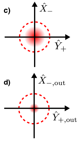
Figure 1: a) The ISTMS setup, consisting of two tunnel-coupled cavities, one of which is coupled to a qubit and the input-output port, and the other flux-pumped by an imbedded SQUID. b) Equivalently, the system can be thought of in terms of its eigenmodes, and the flux-pumping results in a two-mode squeezing interaction between them. c) intracavity and d) output state within the squeezed squeezed subspace defined by joint quadratures of the cavity normal modes (c.f. Eq. (3)), in the absence of any coupling to the qubit. The plots show that when compared to the vacuum state (dashed circle) the intracavity state is never squeezed by more than a factor of two, while the output state can be arbitrarily squeezed.

The remarkable enhancement of measurement in weakly coupled systems is not just of academic interest. Weakly coupled qubit-cavity systems are an emerging topic of current research, with recent developments in the coupling of a single-electron spin to a microwave cavity Petersson2012 ; Viennot2015 ; Stockklauser2015 having projected best-case coupling strengths that are much weaker than typical cavity dissipation rates, putting them firmly in the weak coupling regime. In addition, new circuit QED designs have been proposed that leverage weak coupling to suppress photon shot noise dephasing Zhang2016 . Our in-situ two-mode squeezing setup (ISTMS) would allow an exponential enhancement of measurement rates in such systems, in a way that would be impossible even if one were able to inject external squeezing perfectly.

Our analysis reveals that our ISTMS setup possesses other highly desirable features. Clearly, one potential drawback of generating squeezing in the measurement cavity is the possibility that the complementary amplified quadrature fluctuations in the cavity will cause extraneous backaction on the qubit. Remarkably, such effects are greatly suppressed in our system, as is standard Purcell decay of the qubit due to simple cavity vacuum fluctuations. This is because of a subtle interference effect, which causes the two-cavity system to act like a built-in Purcell filter.

II ISTMS Setup

We start with a setup that is somewhat analogous to the successful Bose-Hubbard dimer amplifier Eichler:2014aa : two tunnel coupled cavities, denoted left and right, where the left cavity has an embedded SQUID, and the right cavity is coupled to an input-output transmission line. To this we add a qubit coupled to the right cavity via a Jaynes-Cummings interaction, and flux-pump the SQUID embedded in the left cavity Yamamoto:2008aa . The ISTMS setup is shown in Fig. 1a).

The Hamiltonian describing this system is ($\hbar=1$ from here on)

$$\hat{H}=\hat{H}_{\rm res}+\hat{H}_{\rm paramp}+\hat{H}_{q}+\hat{H}_{\rm JC}$$ (1)

where $\hat{H}_{\rm res}=\omega_{c}\hat{a}_{L}^{\dagger}\hat{a}_{L}+\omega_{c}\hat{a}_{R}^{\dagger}\hat{a}_{R}+J\left(\hat{a}_{L}^{\dagger}\hat{a}_{R}+\hat{a}_{R}^{\dagger}\hat{a}_{L}\right)$ describes the tunnel coupled cavities (coupling strength $J$), with $\hat{a}_{L/R}$ ($\hat{a}_{L/R}^{\dagger}$) the lowering (raising) operators for the left/right cavities. $\hat{H}_{q}=\omega_{q}\hat{\sigma}_{z}/2$ is the qubit self-Hamiltonian, and $\hat{H}_{\rm JC}=g\left(\hat{a}_{R}^{\dagger}\hat{\sigma}^{-}+\hat{\sigma}^{+}\hat{a}_{R}\right)$ is the Jaynes-Cummings coupling between the qubit and the right cavity. Here $\hat{\sigma}_{z}$ is the Pauli-Z matrix describing the qubit energy eigenstates, and $\hat{\sigma}^{\pm}$ are the raising and lowering operators for the qubit.

Finally, $\hat{H}_{\rm paramp}=i\lambda e^{i\omega_{p}t}\hat{a}_{L}^{2}+h.c.$ is the parametric drive on the left cavity (amplitude $\lambda$) induced by flux-pumping the embedded SQUID at a frequency $\omega_{p}$ Yamamoto:2008aa . In the simplest setup, higher-order cavity nonlinearities will also be induced by the flux-pumped SQUID for large enough drive amplitude $\lambda$. However, in contemporary experiments the effective nonlinearity is reduced, either by introducing an additional linear inductance in the circuit, or by using a SQUID array, such that even up to strong drive amplitudes only the parametric term is relevant Eichler:2014aa ; Eichler2014 .

As we focus on the regime where $J\gg g,\lambda$ the tunnel-coupled cavities are best described by their eigenmodes, $\hat{a}_{E}=(\hat{a}_{L}+\hat{a}_{R})/\sqrt{2}$, $\hat{a}_{O}=(\hat{a}_{R}-\hat{a}_{L})/\sqrt{2}$, which we refer to as the even and odd modes (see Fig. 1(b)). The corresponding normal mode frequencies are $\omega_{E/O}=\omega_{c}\pm J$ . The flux pumping of the left cavity results in a two-mode squeezing interaction between these eigenmodes, which is resonant for $\omega_{p}=2\omega_{c}$.

We move into an interaction picture, such that each cavity normal mode frequency is shifted to zero. Setting $\omega_{q}=\omega_{c}$, we then make a standard dispersive transformation to eliminate the qubit-cavity interaction to leading order; here, $J$ plays the role of a large cavity-qubit detuning. This results in the Hamiltonian

$$\hat{H}_{D}=\chi\left(\hat{a}_{E}^{\dagger}\hat{a}_{E}-\hat{a}_{O}^{\dagger}\hat{a}_{O}\right)\hat{\sigma}_{z}-i\lambda\left(\hat{a}_{E}\hat{a}_{O}-\hat{a}^{\dagger}_{E}\hat{a}^{\dagger}_{O}\right),$$ (2)

where $\chi=g^{2}/(2J)$ is the dispersive coupling, and where we have neglected terms that are higher-order in powers of $g/J,\lambda/J$. We have also used the condition $\lambda/J\ll 1$ to allow a rotating wave approximation where non-resonant terms coming from the parametric drive are dropped (see A and B for more details).

Eq. (2) shows clearly that the qubit is dispersively coupled to both cavity normal modes, with dispersive couplings that only differ in sign. As discussed in Ref. Didier2015 , this situation is highly advantageous if one wants to exploit squeezing, as it gives rise to a dynamical symmetry that has been termed a “quantum mechanics free subspace” Tsang:2012aa ; we discuss this more below. Unlike Ref. Didier2015 , this symmetry is achieved without having to explicitly engineer two distinct qubit-cavity couplings, giving us a distinct practical advantage.

The coupling between the right cavity to its readout transmission line is described using standard input-output theory QuantumNoise , with an energy decay rate $2\kappa$. Hence, the decay rate for each of the normal modes is $\kappa$. Focusing on the case $J\gg\kappa$, the $\hat{a}_{E}$ and $\hat{a}_{O}$ modes are well resolved in frequency, and thus each couple to an independent set of transmission line modes (see C).

To understand how our system can be used for dispersive qubit readout we define $\hat{a}_{\pm}=(\hat{a}_{E}\pm\hat{a}_{O})/\sqrt{2}$ (in our interaction picture), and rewrite Eq. (2) in terms of the quadrature operators $\hat{X}_{\pm}=(\hat{a}_{\pm}+\hat{a}_{\pm}^{\dagger})/\sqrt{2}$ and $\hat{Y}_{\pm}=-i(\hat{a}_{\pm}-\hat{a}_{\pm}^{\dagger})/\sqrt{2}$

$$\hat{H}_{D}=\chi\left(\hat{X}_{+}\hat{X}_{-}+\hat{Y}_{+}\hat{Y}_{-}\right)\hat{\sigma}_{z}+\lambda\left(\hat{X}_{+}\hat{Y}_{+}-\hat{X}_{-}\hat{Y}_{-}\right).$$ (3)

The first term in this Hamiltonian describes a quantum-mechanics-free subsystem interaction Didier2015 ; Tsang:2012aa that mediates a qubit dependent rotation in the effective phase-space plane defined by $\{\hat{X}_{-},\hat{Y}_{+}\}$. A coherent driving of the $\hat{Y}_{+}$ quadrature will be rotated by the interaction with the qubit, resulting in a non-zero value of $\langle\hat{X}_{-}\rangle$ that is qubit state dependent. This can be detected via a homodyne measurement of the output field leaving the cavity, thus measuring the state of the qubit.

The second term in Eq. (3) describes the generation of in-situ squeezing that is unique and so crucial to our setup. It effectively damps both the $\{\hat{X}_{-},\hat{Y}_{+}\}$ quadratures without adding noise, thereby generating intracavity two-mode squeezing. While the intracavity squeezing remains weak, the squeezing of the output field quadratures can be much stronger, due to the well-known interference between the noise leaving the cavity and the vacuum noise that is promptly reflected at the cavity entrance QuantumNoise , as is shown in Fig. 1c) and d). The net result is that the vacuum noise is strongly reduced in any linear combination of $\{\hat{X}_{-},\hat{Y}_{+}\}$ quadratures, and in particular the combination that has maximal information on the qubit state. Unlike schemes using single-mode squeezing and dispersive interactions, one never has to worry about the anti-squeezed quadrature corrupting the measurement results.

While for $\chi=0$, Eq. (3) can produce arbitrarily large amounts of output two mode squeezing as one approaches the parametric instability at $\lambda=\kappa/2$, for non-zero $\chi$, the interaction with the qubit will disrupt the needed interference. The result is a double-peaked squeezing spectrum, with Lorentzian peaks at $\omega=\pm\chi$ (see Fig. 2). This effect is negligible for weak coupling, and even at stronger couplings the output noise remains squeezed below zero point. We stress that the interaction with the qubit never causes a mixing of squeezed and anti-squeezed quadratures (as occurs if one simply injects single-mode squeezing into a dispersively-coupled readout cavity Barzanjeh2014 ; Didier2015 ).

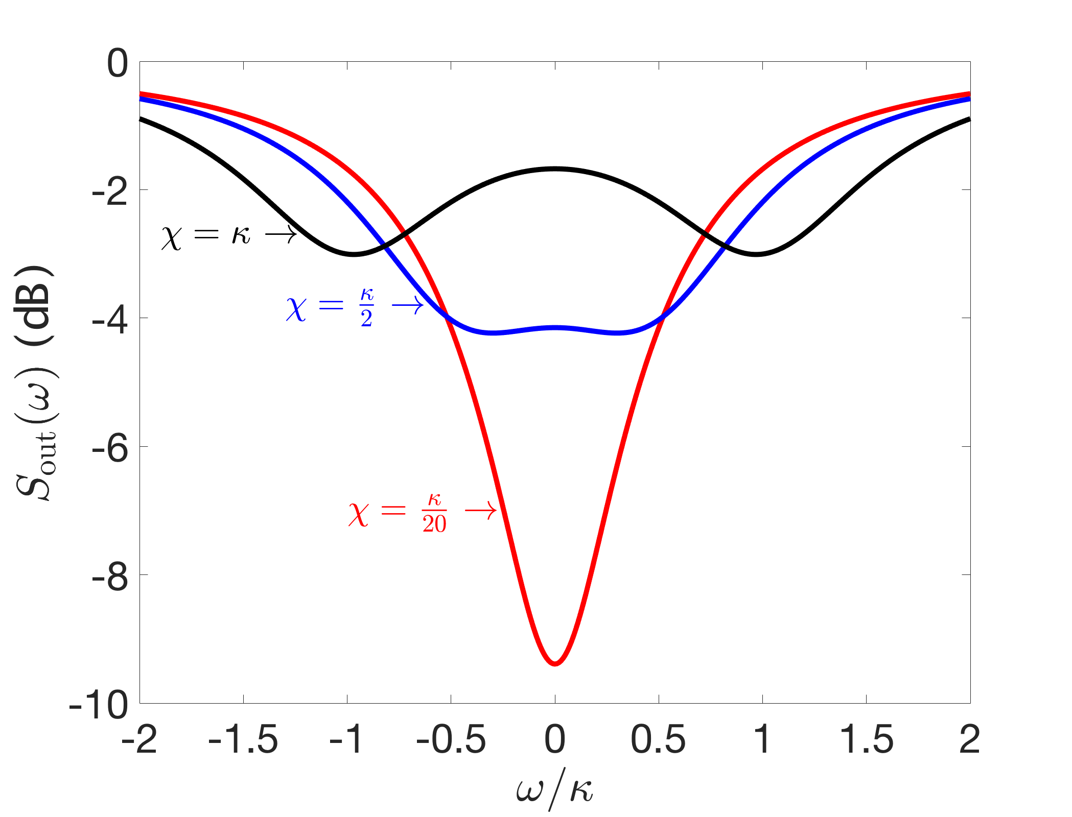
Figure 2: Output squeezing spectrum of the joint quadrature $\hat{X}_{-,{\rm out}}=\left(\hat{X}_{E,{\rm out}}+\hat{X}_{O,{\rm out}}\right)/\sqrt{2}$ for the ISTMS setup (see C), with $\lambda=\kappa/4$. As $\chi\rightarrow 0$ the spectrum approaches a single Lorentzian, while for stronger coupling it is the sum of two Lorentzians centered at $\pm\chi$. Even for strong coupling the noise is always squeezed below zero point, as the qubit back-action does not mix amplified noise into the output.

III Measurement rate in the long time limit

We first consider the measurement properties of our system in the limit where one integrates the homodyne current associated with the cavity output field for a time $\tau\gg 1/\kappa$. In this limit, the SNR generically behaves as $\sqrt{\Gamma\tau}$, where $\Gamma$ is the measurement rate (i.e. the rate at which information is obtained on the qubit state) Clerk:2010aa . For a standard dispersive readout (i.e. a single cavity and a simple coherent state drive), one makes a homodyne measurement of the output phase quadrature. The measurement rate satisfies

$$\Gamma_{\rm SM}=\Bigg{\{}\begin{array}[]{ll}4\bar{n}\kappa,&{\rm if}\ \chi=\kappa/2\\ 2\bar{n}\left(\chi/\kappa\right)^{2}\kappa,&{\rm if}\ \chi\ll\kappa/2.\end{array}$$ (6)

Here $\bar{n}$ is the average intracavity photon number induced by the coherent driving of the cavity. The first line represents the optimal case, where one has a strong, optimally tuned cavity-qubit coupling. The second line is the result for a weakly coupled qubit. One cannot increase $\bar{n}$ without bound to increase $\Gamma_{\rm SM}$ for weak coupling, as $\bar{n}$ is bounded by the critical photon number Blais2004 , above which detrimental back-action on the qubit occurs. Hence, new ideas are needed to overcome the slow measurement rates associated with weakly-coupled qubits.

We now turn to our ISTMS setup. The measurement again involves coherently driving the cavity, and integrating the appropriate output homodyne current for a time $\tau$. The coherent drive should displace the cavity $\hat{Y}_{E/O}$ quadratures, while the output homodyne measurement corresponds to monitoring the $\hat{X}_{-}$ collective quadrature. The parametric drive $\lambda$ is kept on during the measurement to generate the desired squeezing (taking $\lambda<\kappa/2$ to ensure the system stays stable). Further details on how the collective quadrature is measured (using standard techniques) are provided in C.

For long integration times, we find that the measurement rate is:

$$\Gamma_{\rm ISTMS}=\frac{8\bar{n}_{0}\chi^{2}}{\chi^{2}+\left(\frac{\kappa}{2}-\lambda\right)^{2}}\kappa,$$ (7)

Here, $\bar{n}_{0}$ is the intracavity photon number associated with the displacement induced by the coherent drive. The total average intracavity photon number $\bar{n}\equiv\langle\hat{a}_{E}^{\dagger}\hat{a}_{E}+\hat{a}_{O}^{\dagger}\hat{a}_{O}\rangle=\bar{n}_{0}+\bar{n}_{\rm sqz}$ also includes a contribution $\bar{n}_{\rm sqz}$ from the squeezing. This is given by $\bar{n}_{\rm sqz}=\lambda^{2}/\left[\left(\kappa/2\right)^{2}-\lambda^{2}\right]$.

IV Weak coupling enhancement

For weak couplings $\chi\ll\kappa$, the qubit-induced disruption of squeezing (i.e. $\chi^{2}$ term in denominator of Eq. (7)) is weak, and the ISTMS scheme enables dramatic enhancements of the measurement rate. To see this, we first note that once the parametric drive is increased past $\lambda\sim\kappa/2-\chi$, $\Gamma_{\rm ISTMS}$ becomes independent of $\lambda$, and saturates to a value that is independent of the dispersive coupling $\chi$. For the threshold value of $\lambda=\kappa/2-\chi$ we have

$$\Gamma_{\rm ISTMS}=4\bar{n}_{0}\kappa.$$ (8)

Strikingly, this expression is independent of the dispersive coupling $\chi$, even if $\chi\ll\kappa$. This result may seem odd, given that it implies a finite measurement rate as $\chi\rightarrow 0$. However, we consider the situation where as $\chi$ decreases the squeezing increases to compensate, such that the measurement rate remains finite.

To understand the significance of this result, we compare it against the measurement rate of a standard dispersive measurement made with the same total number of intracavity photons, but where the qubit coupling is increased to its optimal value $\chi\rightarrow\kappa/2$. We find:

$$\frac{\Gamma_{\rm ISTMS}[\chi\ll\kappa]}{\Gamma_{\rm SM,opt}[\chi=\kappa/2]}=\frac{\bar{n}_{0}}{\bar{n}_{0}+\frac{\kappa}{4\chi}}$$ (9)

If the ISTMS measurement is made with a sufficiently large coherent drive (such that that $\bar{n}_{0}\gg\kappa/\chi$), the measurement rate for a weakly coupled qubit can match the maximum measurement rate of a standard dispersive measurement (something that necessarily requires strong coupling).

Squeezing in the ISTMS scheme thus lets one in principle completely overcome the limitation of having a weakly coupled qubit without having to compensate with an extremely large number of measurement photons. This is also accomplished without having to transport and inject an externally prepared squeezed state into a cavity with high efficiency. We stress that this optimal scaling is not possible in a standard single-cavity setup, even if one could perfectly inject externally-generated single-mode squeezing; this is because the interaction with the qubit always mixes squeezed and anti-squeezed quadratures Barzanjeh2014 ; Didier2015 , something that does not happen in our scheme (c.f. Fig. 2).

V Short-time measurement dynamics

While our discussion so far focused on the long-time properties of a measurement (as described by the measurement rate), the ISTMS setup also provides strong advantages for finite measurement times. We quantify the speed of readout by the measurement time required to reach $99.99\%$ fidelity, $\tau^{*}$. The fidelity is given by $F=1-{\rm erfc}({\rm SNR}/2)/2$, where SNR denotes the signal-to-noise ratio. We will be interested in situations where $\tau^{*}\kappa$ is finite, and thus use in what follows the full expression for the time-dependent SNR (which reflects the non-white output noise spectrum) found in C.

We find that for weak couplings $\chi\ll\kappa$, the qubit-induced squeezing disruption is minimal, and the ISTMS scheme results in substantial reductions of $\tau^{*}$ compared to a standard dispersive measurement made with the same coupling and average intracavity photon number. This is shown explicitly in Fig. 3. For weak couplings $\chi=10^{-2}\kappa$, the ISTMS scheme results in an almost five-fold reduction in $\tau^{*}$ in the limit of large $\bar{n}_{0}$.

Despite the large $\bar{n}_{0}$, the total intracavity photon number is below the critical photon number, which is given by $n_{\rm crit}=J/4\chi$ for the ISTMS setup. For a realistic $J=10\kappa$, this gives $n_{\rm crit}=25,\ 50,\ 250$, for $\kappa/\chi=10,\ 20,\ 100$. As we are below $n_{\rm crit}$, we do not expect to see the effects of higher-order nonlinearities arising from the full Jaynes-Cummings interaction, and furthermore, there is a mounting body of evidence that even as one approaches $n_{\rm crit}$, the state of the system is not greatly affected Jeffrey:2014zr ; Khezri:2016aa ; Sank:2016aa . In support of this intuition, a numerical comparison to the full Jaynes-Cummings model is discussed in D.

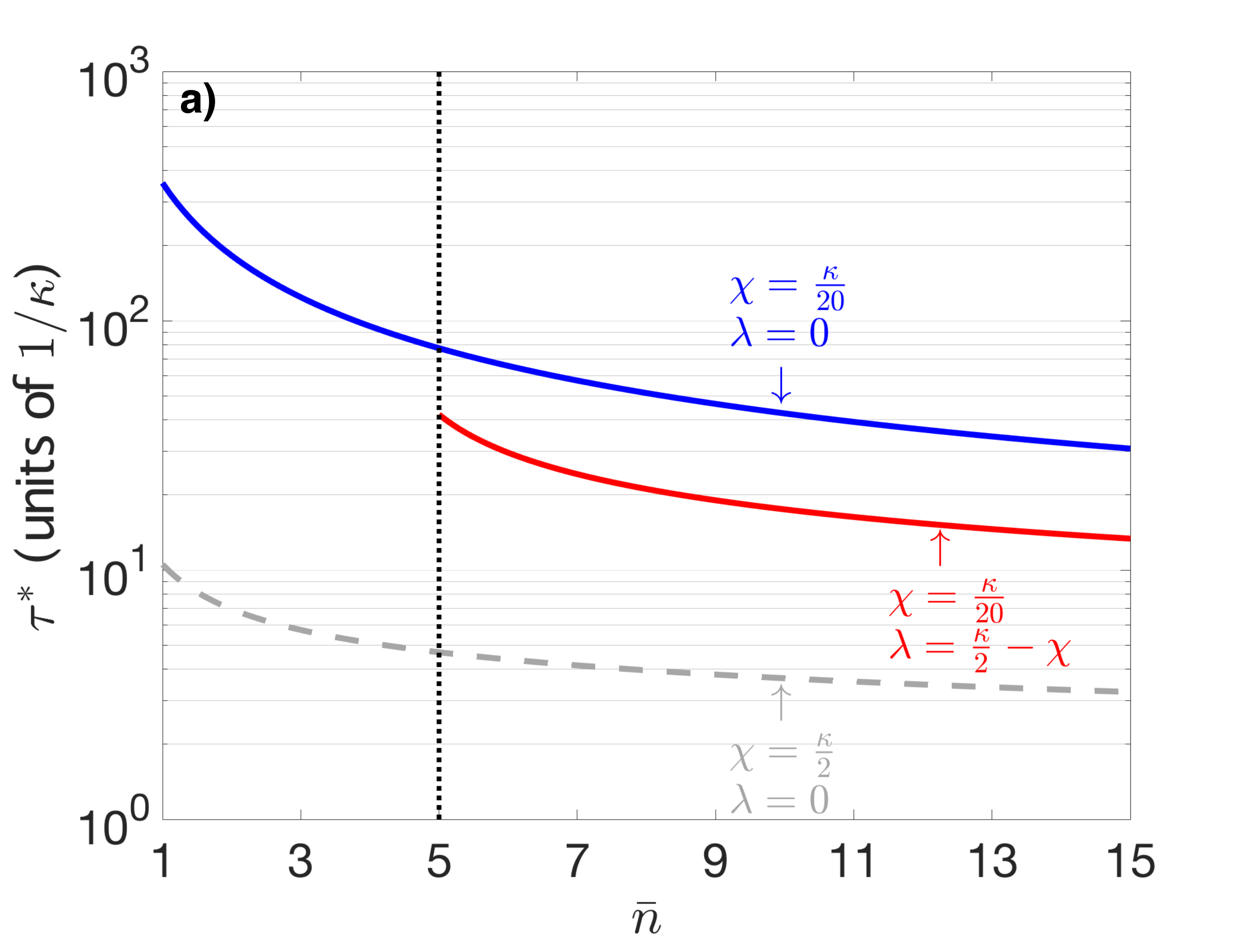
Figure 3: a) Measurement time $\tau^{*}$ needed for a fidelity $F=0.9999$ as a function of total intracavity photon number. Solid curves correspond to a weak qubit-cavity coupling $\chi=\kappa/20$, while the dashed curve describes an optimal strong coupling $\chi=\kappa/2$. For the ISTMS setup (red curve) the number of squeezing photons $n_{\rm sqz}\approx 4$, indicated by the dotted vertical line. b) Ratio of $\tau^{*}$ for standard readout with zero squeezing to that for the ISTMS setup with $\lambda=\kappa/2-\chi$. $\tau^{*}$ can be reduced almost five-fold for the weakest coupling.

VI Effect of losses

While the ISTMS setup does not suffer from the problems associated with transporting and injecting a squeezed state, its efficacy will be degraded if there are significant internal cavity losses $\kappa_{\rm int}$. Taking both cavities to have the same level of internal loss, and letting $\varepsilon=\kappa_{\rm int}/({\kappa_{\rm int}+\kappa})$, we find that the weak-coupling measurement rate in Eq. (8) (which is independent of coupling) is not modified by internal loss as long as $(\chi/\kappa)^{2}>\varepsilon/2$; in this regime the reductions in measurement time depicted in Fig. 3 are also not significantly impacted. Further details on the effects of internal losses (and external measurement efficiencies) are presented in E.

VII Suppression of Purcell decay and other extraneous qubit backaction

An obvious concern with the ISTMS setup is that anti-squeezing generated by the parametric drive will greatly enhance non-QND backaction effects on the qubit. In a standard dispersive setup, the non-QND backaction corresponds to Purcell decay, the cavity-enhanced relaxation of the qubit excited state Blais2004 . In our setup, one might expect that the parametric driving enhances both the cavity-induced qubit decay and qubit heating.

Remarkably, these are not issues in the ISTMS setup. This is the result of an interference effect involving the two cavities in the setup that cause it to act as its own, intrinsic Purcell filter, thus removing the necessity to construct an external filter Reed2010 ; Jeffrey:2014zr ; Govia:2015aa ; Bronn:2015aa . Heuristically, vacuum noise entering the right cavity can either drive the even or odd cavity normal mode before reaching the qubit (see Fig. 4). The interference between these possibilities is perfectly destructive at the qubit frequency (which is at the average to the two cavity normal mode frequencies). Formally, this results in a suppression of the effective photonic density of states seen by the qubit (see Fig. 4 and F).

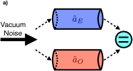
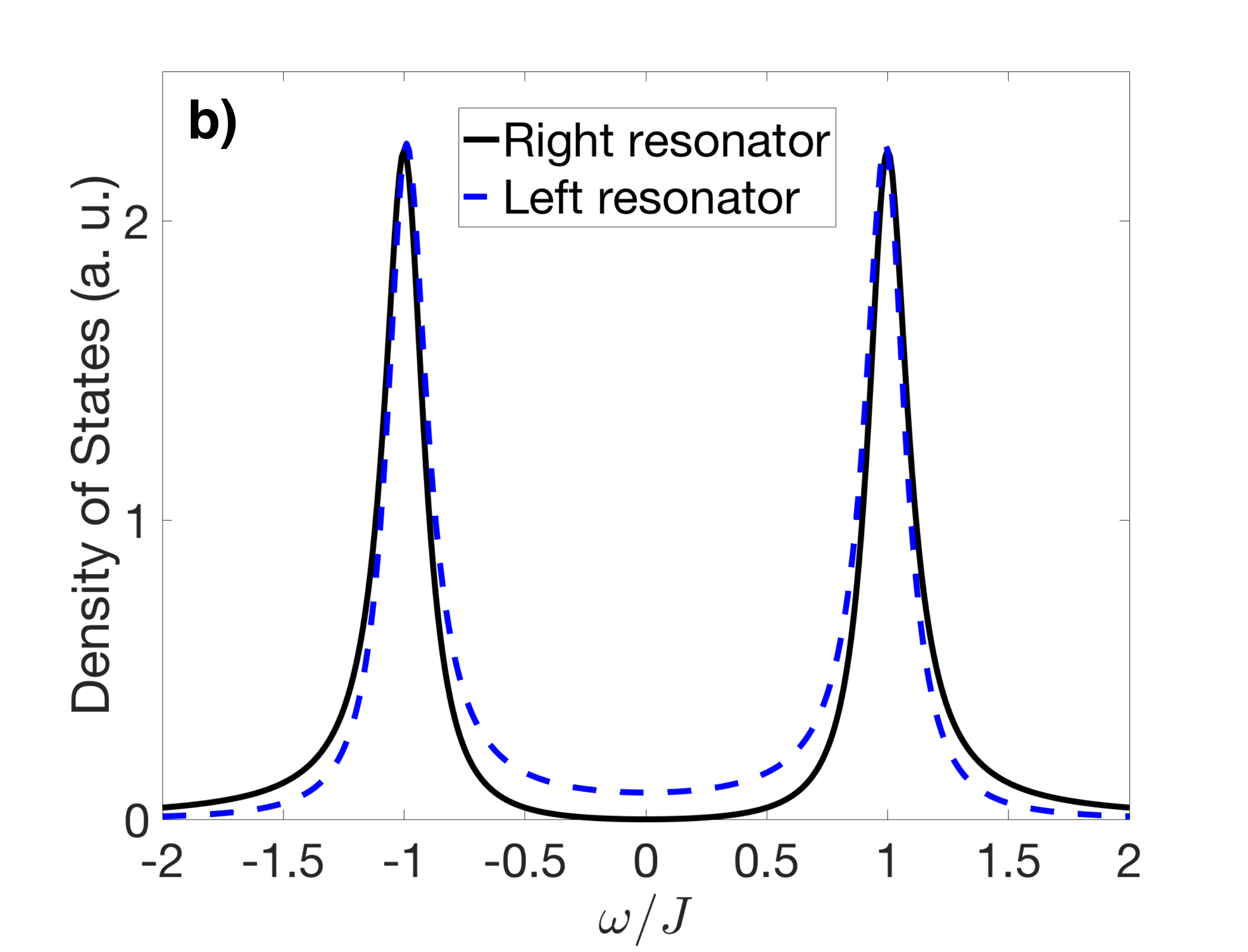
Figure 4: a) Schematic of the destructive interference leading to cancelation of the vacuum noise at the qubit frequency. b) Density of states (see F) of the right and left cavities for $\lambda=0$ and $J=5\kappa$. Due to quantum noise interference the DoS of the right cavity is exactly zero at the qubit frequency ($\omega=0$ in this frame).

Alternatively, one can understand the effect by considering how the cavity normal modes transform under the dispersive transformation. One finds to leading order in $1/J$

$$\hat{\tilde{a}}_{E/O}\simeq\hat{a}_{E/O}+\frac{g}{\sqrt{2}J}\left(\mp\hat{\sigma}^{-}+\frac{\lambda}{J}\hat{\sigma}^{+}\right),$$ (10)

where $\hat{\tilde{a}}_{E/O}$ denotes the transformed version of the original normal mode lowering operators $\hat{a}_{E/O}$ . As is standard, the weak hybridization of the qubit and cavity modes cause $\hat{\tilde{a}}_{E/O}$ to acquire a term involving the qubit lowering operator $\hat{\sigma}^{-}$. More unusual is the fact that these operators also mix with the qubit raising operator $\hat{\sigma}^{+}$ due to the parametric drive $\lambda$.

The transmission line coupled to the right cavity couples to $\hat{a}_{R}$ via a system-bath coupling Hamiltonian of the form $\hat{H}_{SB}=\sqrt{2\kappa}\hat{B}^{\dagger}\hat{a}_{R}+h.c.$, where $\hat{B}^{\dagger}$ is a bath operator that creates an excitation in the transmission line (see, e.g., Clerk:2010aa ). In the dispersive frame, $\hat{a}_{R}$ becomes:

$$\hat{\tilde{a}}_{R}=\frac{\hat{\tilde{a}}_{E}+\hat{\tilde{a}}_{O}}{\sqrt{2}}\simeq\frac{\hat{a}_{E}+\hat{a}_{O}}{\sqrt{2}}+\frac{g\lambda}{J^{2}}\hat{\sigma}^{+}.$$ (11)

Note that the $\hat{\sigma}^{-}$ perfectly cancels in this expression. As a result, there is no amplitude for creating a bath excitation (via $\hat{B}^{\dagger}$) and relaxing the qubit, meaning that conventional Purcell decay is suppressed.

In contrast, there is a weak amplitude for both creating a bath excitation and exciting the qubit. The corresponding heating rate of the qubit is readily found to be $\gamma_{H}=\kappa\left(g\lambda/J^{2}\right)^{2}$. This heating is an example of “quantum heating”, as discussed in Refs. Dykman:2011aa ; Marthaler:2006aa . While this heating is clearly unwanted, we stress that it is much weaker that standard Purcell decay in the regime of interest: standard Purcell decay would scale as $(g/J)^{2}\kappa$, where as the above heating effect is suppressed by an additional extremely small parameter $(\lambda/J)^{2}<(\kappa/2J)^{2}$, with $(\kappa/2J)^{2}\sim 1/100$ achievable for realistic values of $J$ Eichler:2014aa . Qubit dissipation effects due to internal loss in the left cavity are treated in F.

VIII Conclusion

We have presented an analysis of a realistic two-cavity setup that allows squeezing to dramatically enhance the readout of weakly-coupled qubits: our setup essentially allows one to recover the optimal measurement rate of a strongly-coupled system while using a weakly-coupled system. This is accomplished in a manner that does not require one to transport and inject an externally-produce squeezed state with high fidelity. The system is also remarkably robust against non-QND backaction effects, due to an interference effect that causes the system to act as its own, intrinsic Purcell filter. There are many possible routes for realizing the parametric drive used in our setup. One could flux-pump a SQUID embedded in the left cavity Yamamoto:2008aa , or use a Josephson-junction mediated coupling to an external pump mode, as has been done to great effect in Josephson parametric converter circuits Bergeal:2010aa ; Bergeal2010 ; Sliwa:2015aa . Finally, while the focus of our work has been on circuit/cavity QED, the ISTMS setup and the results obtained here are completely general, and can be applied to other physical systems, such as optomechanics Peano:2015aa .

IX Acknowledgements

This work was supported by the Army Research Office under Grant No. W911NF-14-1-0078.

Appendices

Appendix A Two-Mode Squeezing

We begin with the Hamiltonian describing two tunnel-coupled cavities, one of which has an embedded SQUID that is flux-pumped at frequency $\omega_{p}$ Yamamoto:2008aa

$$\hat{H} =\omega_{c}\hat{a}_{L}^{\dagger}{a}_{L}+\omega_{c}\hat{a}_{R}^{\dagger}{a}_{R}+J\left(\hat{a}_{L}^{\dagger}\hat{a}_{R}+\hat{a}_{R}^{\dagger}\hat{a}_{L}\right)$$

$$+i\lambda\left(e^{i\omega_{p}t}-e^{-i\omega_{p}t}\right)\left(\hat{a}_{L}-\hat{a}_{L}^{\dagger}\right)^{2},$$ (12)

where $J$ is the tunnel coupling strength and $\lambda$ is the strength of the flux pump. We define the eigenmodes of the coupled cavities as

$$\hat{a}_{E}=\frac{\hat{a}_{L}+\hat{a}_{R}}{\sqrt{2}},\ \ \hat{a}_{O}=\frac{\hat{a}_{R}-\hat{a}_{L}}{\sqrt{2}}.$$ (13)

In this basis, the Hamiltonian is given by

$$\hat{H} =\omega_{E}\hat{a}_{E}^{\dagger}{a}_{E}+\omega_{O}\hat{a}_{O}^{\dagger}{a}_{O}$$

$$+\frac{i\lambda}{2}\left(e^{i\omega_{p}t}-e^{-i\omega_{p}t}\right)\left(\hat{a}_{E}-\hat{a}_{O}-\hat{a}_{E}^{\dagger}+\hat{a}_{O}^{\dagger}\right)^{2},$$ (14)

where $\omega_{E}=\omega_{c}+J$ and $\omega_{O}=\omega_{c}-J$. Defining $\hat{A}=\left(\hat{a}_{E}-\hat{a}_{O}-\hat{a}_{E}^{\dagger}+\hat{a}_{O}^{\dagger}\right)^{2}$ and expanding we have

$$\hat{A}=\hat{a}_{E}\hat{a}_{E}+\hat{a}_{O}\hat{a}_{O}+\hat{a}^{\dagger}_{E}\hat{a}^{\dagger}_{E}+\hat{a}^{\dagger}_{O}\hat{a}^{\dagger}_{O}-2\hat{a}_{E}\hat{a}_{O}$$

$$-2\hat{a}^{\dagger}_{E}\hat{a}^{\dagger}_{O}-2\hat{a}^{\dagger}_{E}\hat{a}_{E}-2\hat{a}^{\dagger}_{O}\hat{a}_{O}+2\hat{a}^{\dagger}_{O}\hat{a}_{E}+2\hat{a}^{\dagger}_{E}\hat{a}_{O},$$ (15)

and in the interaction frame this becomes

$$\hat{A}_{I}=\ e^{-2i\omega_{E}t}\hat{a}_{E}\hat{a}_{E}+e^{-2i\omega_{O}t}\hat{a}_{O}\hat{a}_{O}+e^{2i\omega_{E}t}\hat{a}^{\dagger}_{E}\hat{a}^{\dagger}_{E}$$

$$+e^{2i\omega_{O}t}\hat{a}^{\dagger}_{O}\hat{a}^{\dagger}_{O}-2\hat{a}^{\dagger}_{E}\hat{a}_{E}-2\hat{a}^{\dagger}_{O}\hat{a}_{O}$$

$$-2e^{-i\left(\omega_{E}+\omega_{O}\right)t}\hat{a}_{E}\hat{a}_{O}-2e^{i\left(\omega_{E}+\omega_{O}\right)t}\hat{a}^{\dagger}_{E}\hat{a}^{\dagger}_{O}$$

$$+2e^{-i\left(\omega_{E}-\omega_{O}\right)t}\hat{a}^{\dagger}_{O}\hat{a}_{E}+2e^{i\left(\omega_{E}-\omega_{O}\right)t}\hat{a}^{\dagger}_{E}\hat{a}_{O}.$$ (16)

Setting $\omega_{p}=2\omega_{c}$, we drop all terms that oscillate rapidly at frequencies on the order of $\omega_{c}\gg J$ in the product $\left(e^{i\omega_{p}t}-e^{-i\omega_{p}t}\right)\hat{A}_{I}$ to arrive at the Hamiltonian in the interaction frame

$$\hat{H}_{I} =-i\lambda\left(\hat{a}_{E}\hat{a}_{O}-\hat{a}^{\dagger}_{E}\hat{a}^{\dagger}_{O}\right)$$

$$+\frac{i\lambda}{2}\left(e^{-i2Jt}\hat{a}_{E}\hat{a}_{E}+e^{i2Jt}\hat{a}_{O}\hat{a}_{O}-h.c.\right).$$ (17)

If $\lambda/(4J)\ll 1$, then we can also drop the single mode squeezing terms to arrive at the final Hamiltonian in the interaction frame

$$\hat{H}_{I}=-i\lambda\left(\hat{a}_{E}\hat{a}_{O}-\hat{a}^{\dagger}_{E}\hat{a}^{\dagger}_{O}\right),$$ (18)

and in the lab frame

$$\hat{H} =\omega_{E}\hat{a}_{E}^{\dagger}{a}_{E}+\omega_{O}\hat{a}_{O}^{\dagger}{a}_{O}$$

$$-i\lambda\left(e^{i2\omega_{c}t}\hat{a}_{E}\hat{a}_{O}-e^{-i2\omega_{c}t}\hat{a}^{\dagger}_{E}\hat{a}^{\dagger}_{O}\right).$$ (19)

Appendix B Dispersive Approximation

We now include coupling between the right cavity and the qubit to the two-mode squeezing Hamiltonian of Eq. (19). In the eigenmode basis and in a frame rotating at $\omega_{c}=\omega_{q}=\omega_{p}/2$ for both eigenmodes and the qubit, the Hamiltonian is given by

$$\hat{H}^{\prime}=J\hat{a}_{E}^{\dagger}{a}_{E}-J\hat{a}_{O}^{\dagger}{a}_{O}-i\lambda\hat{a}_{E}\hat{a}_{O}+i\lambda\hat{a}^{\dagger}_{E}\hat{a}^{\dagger}_{O}$$

$$+\frac{g}{\sqrt{2}}\left(\hat{a}_{E}^{\dagger}\hat{\sigma}^{-}+\hat{\sigma}^{+}\hat{a}_{E}\right)+\frac{g}{\sqrt{2}}\left(\hat{a}_{O}^{\dagger}\hat{\sigma}^{-}+\hat{\sigma}^{+}\hat{a}_{O}\right).$$ (20)

We make a Schrieffer-Wolff transformation via the generator $S=S_{E}+S_{O}$, where

$$S_{E}=u\hat{a}_{E}\hat{\sigma}^{+}+v\hat{a}_{E}\hat{\sigma}^{-}-u^{*}\hat{a}_{E}^{\dagger}\hat{\sigma}^{-}-v^{*}\hat{a}_{E}^{\dagger}\hat{\sigma}^{+},$$ (21)

$$S_{O}=n\hat{a}_{O}\hat{\sigma}^{+}+m\hat{a}_{O}\hat{\sigma}^{-}-n^{*}\hat{a}_{O}^{\dagger}\hat{\sigma}^{-}-m^{*}\hat{a}_{O}^{\dagger}\hat{\sigma}^{+},$$ (22)

with

$$u=-n=-\frac{g}{\sqrt{2}J}\left(1+\frac{\lambda^{2}}{J^{2}}\right)^{-1},$$ (23)

$$v=m=\frac{ig\lambda}{\sqrt{2}J^{2}}\left(1+\frac{\lambda^{2}}{J^{2}}\right)^{-1},$$ (24)

chosen to cancel terms of order $g$ in the transformed Hamiltonian. Keeping only terms up to second order in $g/J$, we obtain the dispersive Hamiltonian

$$\hat{H}_{D} =J\hat{a}_{E}^{\dagger}{a}_{E}-J\hat{a}_{O}^{\dagger}{a}_{O}+\chi\left(\hat{a}_{E}^{\dagger}{a}_{E}-\hat{a}_{O}^{\dagger}{a}_{O}\right)\hat{\sigma}_{z}$$

$$-i\lambda\left(1-\frac{\chi}{J}\hat{\sigma}_{z}\right)\left(\hat{a}_{E}\hat{a}_{O}-\hat{a}^{\dagger}_{E}\hat{a}^{\dagger}_{O}\right)$$

$$+\frac{i\lambda\chi}{2J}\left(1-\frac{\chi}{J}\hat{\sigma}_{z}\right)\left(\hat{a}_{E}^{2}-(\hat{a}_{E}^{\dagger})^{2}\right)\hat{\sigma}_{z}$$

$$+\frac{i\lambda\chi}{2J}\left(1-\frac{\chi}{J}\hat{\sigma}_{z}\right)\left(\hat{a}_{O}^{2}-(\hat{a}_{O}^{\dagger})^{2}\right)\hat{\sigma}_{z}.$$ (25)

where

$$\chi=\frac{g^{2}}{2J}\left(1+\frac{\lambda^{2}}{J^{2}}\right)^{-1},$$ (26)

which we approximate as $\chi=g^{2}/2J$ in the main text as $\lambda/J$ is a small parameter. As a result of the fact that the qubit frequency is placed exactly midway between the two cavity eigenmode frequencies, there is no second order qubit-mediated eigenmode coupling due to destructive interference.

The terms in the last two lines of Eq. (25) are single mode squeezing terms for each eigenmode. However, these terms are both off resonance and are damped by the small parameter $\chi/2J$. Therefore, provided $\lambda\chi/(4J^{2})\ll 1$ they can be safely ignored, and one obtains the dispersive Hamiltonian used in the main text.

Appendix C Measurement Dynamics and Signal-to-Noise Ratio

Starting from the Hamiltonian in the dispersive frame (Eq. (2) of the main text) we derive the equations of motion for the even and odd modes

$$\dot{\hat{a}}_{E}=-i\chi\hat{\sigma}_{z}\hat{a}_{E}+\lambda\hat{a}_{O}^{\dagger}-\frac{\kappa}{2}\hat{a}_{E}-\sqrt{\kappa}\hat{b}_{E,{\rm in}}(t),$$ (27)

$$\dot{\hat{a}}_{O}=i\chi\hat{\sigma}_{z}\hat{a}_{O}+\lambda\hat{a}_{E}^{\dagger}-\frac{\kappa}{2}\hat{a}_{O}-\sqrt{\kappa}\hat{b}_{O,{\rm in}}(t),$$ (28)

where $\kappa$ is the decay rate of the eigenmodes into the transmission line, and $\hat{b}_{E/O,{\rm in}}(t)$ are the input fields for each eigenmode. The above equations are obtained in the limit $J\gg\kappa$ where the environments of the even and odd modes can be treated as independent, as the even and odd modes effectively couple to orthogonal collections of modes in the right transmission line due to their large frequency separation, $2J$, and small linewidth, $\kappa$. For the purpose of calculating the SNR we need only consider the qubit in a definite state, and as such we will write $\hat{\sigma}_{z}$ as a real number $\sigma=\pm 1$ from here on.

In terms of the quadratures of the plus and minus modes, the system evolution equations are

$$\dot{\hat{X}}_{+}=\chi\sigma\hat{Y}_{-}+(\lambda-\frac{\kappa}{2})\hat{X}_{+}-\sqrt{\kappa}\hat{X}_{+,{\rm in}}(t),$$ (29)

$$\dot{\hat{X}}_{-}=\chi\sigma\hat{Y}_{+}-(\lambda+\frac{\kappa}{2})\hat{X}_{-}-\sqrt{\kappa}\hat{X}_{-,{\rm in}}(t),$$ (30)

$$\dot{\hat{Y}}_{+}=-\chi\sigma\hat{X}_{-}-(\lambda+\frac{\kappa}{2})\hat{Y}_{+}-\sqrt{\kappa}\hat{Y}_{+,{\rm in}}(t),$$ (31)

$$\dot{\hat{Y}}_{-}=-\chi\sigma\hat{X}_{+}+(\lambda-\frac{\kappa}{2})\hat{Y}_{-}-\sqrt{\kappa}\hat{Y}_{-,{\rm in}}(t),$$ (32)

with the input quadratures defined appropriately. We will focus on the squeezed quadratures $\hat{X}_{-}$ and $\hat{Y}_{+}$, whose evolution is decoupled from that of the amplified quadratures. In frequency space, the solutions for the squeezed quadratures are given by

$$\left(\begin{array}[]{c}\hat{X}_{-}(\omega)\\ \hat{Y}_{+}(\omega)\end{array}\right)=\frac{-\sqrt{\kappa}}{(\lambda+\frac{\kappa}{2}+i\omega)^{2}+\chi^{2}}\left(\begin{array}[]{cc}i\omega+\lambda+\frac{\kappa}{2}&-\chi\sigma\\ \chi\sigma&i\omega+\lambda+\frac{\kappa}{2}\end{array}\right)\left(\begin{array}[]{c}\hat{X}_{-,{\rm in}}(\omega)\\ \hat{Y}_{+,{\rm in}}(\omega)\end{array}\right)$$ (39)

and using the usual input-output relation $\hat{X}_{-,{\rm out}}(\omega)=\hat{X}_{-,{\rm in}}(\omega)+\sqrt{\kappa}\hat{X}_{-}(\omega)$, we can calculate the output field of the $\hat{X}_{-}$ quadrature in frequency space

$$\hat{X}_{-,{\rm out}}(\omega) =\left(1-\frac{\kappa(\lambda+\frac{\kappa}{2}+i\omega)}{(\lambda+\frac{\kappa}{2}+i\omega)^{2}+\chi^{2}}\right)\hat{X}_{-,{\rm in}}(\omega)$$

$$+\frac{\kappa\chi\sigma}{(\lambda+\frac{\kappa}{2}+i\omega)^{2}+\chi^{2}}\hat{Y}_{+,{\rm in}}(\omega).$$ (40)

C.1 Measurement Protocol

We consider a homodyne measurement, for which the homodyne current will be proportional to the average value of the output quadrature $\hat{X}_{-,{\rm out}}(t)$. It is important to note that while the measurement signal is contained in only one quadrature, $\hat{X}_{-,{\rm out}}(t)$, this quadrature exists in a frame rotating at different frequencies for the two cavities, and cannot be directly measured. The physical measurement requires measuring the homodyne currents for both the even and odd modes, i.e. $\left<\hat{X}_{E,{\rm out}}(t)\right>$ and $\left<\hat{X}_{O,{\rm out}}(t)\right>$, which are separated in frequency by $2J$. Calculation of $\left<\hat{X}_{-,{\rm out}}(t)\right>$ can then be done via classical post processing of these signals. As input we consider $\left<\hat{Y}_{+,{\rm in}}(t)\right>\neq 0$ and $\left<\hat{X}_{-,{\rm in}}(t)\right>=0$, such that in light of Eq. (40), $\left<\hat{X}_{-,{\rm out}}(t)\right>$ will be qubit-state dependent. As was the case for the measurement quadrature, the input quadrature $\hat{Y}_{+,{\rm in}}(t)$ cannot be directly accessed, so the physical input will consist of coherently driving both input modes, $\hat{Y}_{E,{\rm in}}(t)$ and $\hat{Y}_{O,{\rm in}}(t)$, such that the correct coherent drive is applied to the combined quadrature $\hat{Y}_{+,{\rm in}}(t)$.

C.2 Measurement Signal

We set

$$\left<\hat{Y}_{+,{\rm in}}(t)\right>=\sqrt{2}\left|\beta\right|\Theta(t-t_{0}),$$ (41)

which describes a coherent pulse incident on the system beginning at time $t_{0}$, which we assume is long after the system has reached its undriven steady-state. Without loss of generality we can set $t_{0}=0$. The factor of $\sqrt{2}$ comes from the fact that we define the input field of the plus mode as $\left<\hat{b}_{+,in}(t)\right>=i\left|\beta\right|\Theta(t-t_{0})$, so that the input is entirely in the $\hat{Y}_{+}$ quadrature. For this choice of input field, the expectation value of the output field is given by

$$\left<\hat{X}^{\sigma}_{-,{\rm out}}(t)\right>=\frac{-\sqrt{2}\kappa\chi\left|\beta\right|\sigma}{\left(\lambda+\frac{\kappa}{2}\right)^{2}+\chi^{2}}\Bigg{[}1$$

$$-\left(\cos\left(\chi t\right)+\frac{\lambda+\kappa/2}{\chi}\sin\left(\chi t\right)\right)e^{-\left(\lambda+\frac{\kappa}{2}\right)t}\Bigg{]}.$$ (42)

We define the measurement operator as $\hat{M}(t)=\hat{X}_{-,{\rm out}}^{+1}(t)-\hat{X}^{-1}_{-,{\rm out}}(t)$, and it is clear from Eq. (42) that the expectation value of this operator is $\left<\hat{M}(t)\right>=2\left<\hat{X}_{-,{\rm out}}^{+1}(t)\right>$. Using this, we calculate the integrated measurement signal

$$\mathcal{M}_{S}(\tau)=\sqrt{\kappa}\int_{0}^{\tau}dt\left<\hat{M}(t)\right>=$$

$$\frac{-2\sqrt{2\bar{n}_{0}}\chi}{\sqrt{\left(\lambda+\frac{\kappa}{2}\right)^{2}+\chi^{2}}}\Bigg{[}\kappa\tau-\frac{\kappa e^{-\left(\lambda+\frac{\kappa}{2}\right)\tau}}{\left(\lambda+\frac{\kappa}{2}\right)^{2}+\chi^{2}}\Bigg{(}\frac{\chi^{2}-(\lambda+\frac{\kappa}{2})^{2}}{\chi}\sin\left(\chi\tau\right)-2\left(\lambda+\frac{\kappa}{2}\right)\left[\cos\left(\chi\tau\right)-e^{\left(\lambda+\frac{\kappa}{2}\right)\tau}\right]\Bigg{)}\Bigg{]},$$ (43)

where we have reparameterized in terms of the coherent intracavity photon number $\bar{n}_{0}$, rather than the input photon flux $\left|\beta\right|$. In the asymptotic long-time limit, $\kappa\tau\gg 1$, the measurement signal can be approximated by

$$\mathcal{M}_{S}(\tau)\rightarrow\frac{-2\sqrt{2\bar{n}_{0}}\chi}{\sqrt{\left(\lambda+\frac{\kappa}{2}\right)^{2}+\chi^{2}}}\kappa\tau.$$ (44)

C.3 Noise

Using Eq. (40) we calculate the output noise to be

$$M^{\sigma}_{N}(t,t^{\prime})=\left<\hat{X}^{\sigma}_{-,{\rm out}}(t)\hat{X}^{\sigma}_{-,{\rm out}}(t^{\prime})\right>=\frac{1}{2}\bigg{(}\delta(t-t^{\prime})$$

$$-\frac{\kappa\lambda}{2(\lambda+\frac{\kappa}{2})}\Big{[}\Theta(t-t^{\prime})e^{-\left(\lambda+\frac{\kappa}{2}\right)(t-t^{\prime})}\left(e^{i\chi(t-t^{\prime})}+e^{-i\chi(t-t^{\prime})}\right)$$

$$+\Theta(t^{\prime}-t)e^{-\left(\lambda+\frac{\kappa}{2}\right)(t^{\prime}-t)}\left(e^{i\chi(t^{\prime}-t)}+e^{-i\chi(t^{\prime}-t)}\right)\Big{]}\bigg{)},$$ (45)

where $\Theta(t-t^{\prime})$ is the Heaviside step function. As expected, the noise is independent of the state of the qubit, and we can suppress the upper index $\sigma$. With this expression we can calculate the integrated noise

$$\mathcal{M}_{N}(\tau)=\kappa\int_{0}^{\tau}dt\int_{0}^{\tau}dt^{\prime}M_{N}(t,t^{\prime})=\frac{1}{2}\left(1-\frac{2\kappa\lambda}{\chi^{2}+\left(\lambda+\frac{\kappa}{2}\right)^{2}}\right)\kappa\tau$$

$$-\frac{\kappa^{2}\lambda}{\left(\lambda+\frac{\kappa}{2}\right)\left[\chi^{2}+\left(\lambda+\frac{\kappa}{2}\right)^{2}\right]^{2}}\Bigg{[}\left(\chi^{2}-\left(\lambda+\frac{\kappa}{2}\right)^{2}\right)\left(1-\cos\left(\chi\tau\right)e^{-\left(\lambda+\frac{\kappa}{2}\right)\tau}\right)-2\chi\left(\lambda+\frac{\kappa}{2}\right)\sin\left(\chi\tau\right)e^{-\left(\lambda+\frac{\kappa}{2}\right)\tau}\Bigg{]},$$ (46)

and in the asymptotic long-time limit this reduces to

$$\mathcal{M}_{N}(\tau)\rightarrow\frac{1}{2}\frac{\chi^{2}+\left(\lambda-\frac{\kappa}{2}\right)^{2}}{\chi^{2}+\left(\lambda+\frac{\kappa}{2}\right)^{2}}\kappa\tau.$$ (47)

C.4 Squeezing Spectrum

The squeezing spectrum is defined by

$$S_{{\rm out}}(\omega)=\int_{0}^{\infty}d\omega^{\prime}\left<\hat{X}_{-,{\rm out}}(\omega)\hat{X}_{-,{\rm out}}(\omega^{\prime})\right>$$ (48)

where $\hat{X}_{-,{\rm out}}(\omega)$ is the Fourier transform of $\hat{X}_{-,{\rm out}}(t)$. For the ISTMS setup, the squeezing spectrum is given by

$$S_{\rm out}(\omega) =\frac{1}{2}\Bigg{(}1-\frac{\kappa\lambda}{\lambda+\frac{\kappa}{2}}\Bigg{[}\frac{\lambda+\frac{\kappa}{2}}{\left(\lambda+\frac{\kappa}{2}\right)^{2}+\left(\omega+\chi\right)^{2}}$$

$$+\frac{\lambda+\frac{\kappa}{2}}{\left(\lambda+\frac{\kappa}{2}\right)^{2}+\left(\omega-\chi\right)^{2}}\Bigg{]}\Bigg{)},$$ (49)

which shows the double-Lorentzian shape seen in the main text. To measure the squeezing spectrum in dB, we compare to the squeezing spectrum for $\lambda=0$, $S_{\rm out}(\omega)=1/2$, using the formula

$$S_{\rm out}(\omega)\ (\rm dB)=10\log_{10}\left[2S_{\rm out}(\omega)\right].$$ (50)

C.5 Signal-to-Noise Ratio

With both the integrated signal and the integrated noise, we can write down the signal to noise ratio

$${\rm SNR}^{2} =\frac{\left(\mathcal{M}_{S}(\tau)\right)^{2}}{\mathcal{M}^{+1}_{N}(\tau)+\mathcal{M}^{-1}_{N}(\tau)}=\frac{\left(\mathcal{M}_{S}(\tau)\right)^{2}}{2\mathcal{M}_{N}(\tau)}$$

$$=\scriptstyle{\frac{\frac{8\bar{n}_{0}\chi^{2}}{\left(\lambda+\frac{\kappa}{2}\right)^{2}+\chi^{2}}\left[\kappa\tau-\frac{\kappa e^{-\left(\lambda+\frac{\kappa}{2}\right)\tau}}{\left(\lambda+\frac{\kappa}{2}\right)^{2}+\chi^{2}}\left(\frac{\chi^{2}-(\lambda+\frac{\kappa}{2})^{2}}{\chi}\sin\left(\chi\tau\right)-2\left(\lambda+\frac{\kappa}{2}\right)\cos\left(\chi\tau\right)\right)-\frac{2\kappa\left(\lambda+\frac{\kappa}{2}\right)}{\left(\lambda+\frac{\kappa}{2}\right)^{2}+\chi^{2}}\right]^{2}}{\frac{\chi^{2}+\left(\lambda-\frac{\kappa}{2}\right)^{2}}{\chi^{2}+\left(\lambda+\frac{\kappa}{2}\right)^{2}}\kappa\tau-\frac{2\kappa^{2}\lambda}{\left(\lambda+\frac{\kappa}{2}\right)\left[\chi^{2}+\left(\lambda+\frac{\kappa}{2}\right)^{2}\right]^{2}}\left[\left(\chi^{2}-\left(\lambda+\frac{\kappa}{2}\right)^{2}\right)\left(1-\cos\left(\chi\tau\right)e^{-\left(\lambda+\frac{\kappa}{2}\right)\tau}\right)-2\chi\left(\lambda+\frac{\kappa}{2}\right)\sin\left(\chi\tau\right)e^{-\left(\lambda+\frac{\kappa}{2}\right)\tau}\right]}}.$$ (51)

In the long-time limit, this becomes

$${\rm SNR}^{2}\rightarrow\frac{8\bar{n}_{0}\chi^{2}}{\chi^{2}+\left(\lambda-\frac{\kappa}{2}\right)^{2}}\kappa\tau.$$ (52)

Appendix D Numerical Comparison of the Jaynes-Cummings and Dispersive Hamiltonians

In order to quantify the effects of higher-order nonlinearities arising from interaction between the qubit and the cavities, we compare the steady-state of the dispersive Hamiltonian we have used in our calculations

$$\hat{H}_{D} =J\hat{a}_{E}^{\dagger}{a}_{E}-J\hat{a}_{O}^{\dagger}{a}_{O}+\chi\left(\hat{a}_{E}^{\dagger}{a}_{E}-\hat{a}_{O}^{\dagger}{a}_{O}\right)\hat{\sigma}_{z}$$

$$-i\lambda\left(\hat{a}_{E}\hat{a}_{O}-\hat{a}^{\dagger}_{E}\hat{a}^{\dagger}_{O}\right),$$ (53)

to that of the full Jaynes-Cummings model

$$\hat{H}^{\prime}=J\left(\hat{a}_{E}^{\dagger}{a}_{E}-\hat{a}_{O}^{\dagger}{a}_{O}\right)-i\lambda\left(\hat{a}_{E}\hat{a}_{O}-\hat{a}^{\dagger}_{E}\hat{a}^{\dagger}_{O}\right)$$

$$+\frac{g}{\sqrt{2}}\left(\hat{a}_{E}^{\dagger}\hat{\sigma}^{-}+\hat{\sigma}^{+}\hat{a}_{E}+\hat{a}_{O}^{\dagger}\hat{\sigma}^{-}+\hat{\sigma}^{+}\hat{a}_{O}\right).$$ (54)

To do so, we numerically calculate the steady-states of the master equations

$$\dot{\rho}=-i\left[\hat{H}_{D},\rho\right]+\kappa\mathcal{D}\left[\hat{a}_{E}\right]\rho+\kappa\mathcal{D}\left[\hat{a}_{O}\right]\rho,$$ (55)

$$\dot{\rho}=-i\left[\hat{H}^{\prime},\rho\right]+\kappa\mathcal{D}\left[\hat{a}_{E}\right]\rho+\kappa\mathcal{D}\left[\hat{a}_{O}\right]\rho,$$ (56)

where $\mathcal{D}\left[x\right]\rho=x\rho x^{\dagger}-\frac{1}{2}\left\{x^{\dagger}x,\rho\right\}$ is the usual dissipator. We have chosen to calculate the numerical steady-states in the even/odd basis, as in this basis the Jaynes-Cummings Hamiltonian can be made time-independent when expressed in a frame rotating at $\omega_{c}$. This makes numerical calculations less computationally intensive than if the Hamiltonian were time-dependent, as the Jaynes-Cummings Hamiltonian would be if expressed in the plus/minus basis. We compare the two steady-states by calculating their fidelity, defined as

$${\rm Fidelity}={\rm Tr}\left(\sqrt{\sqrt{\rho_{D}}\rho_{JC}\sqrt{\rho_{D}}}\right).$$ (57)

It is important to note that the Jaynes-Cummings and dispersive Hamiltonians are connected by a unitary transformation that “mixes” qubit and cavity observables, and as such the steady-states in the two frames are strictly speaking not directly comparable. However, based on previous work Govia:2016aa ; Khezri:2016aa , the scale of the lowest order effect of this mixing is set by $\chi/J$, and for our parameter choice ($\chi/J=1/200$) this will have only a small effect on a direct comparison of the steady-states. Additionally, as we are primarily interested in the effect the Jaynes-Cummings dynamics has on the cavity state, we treat the even and odd mode decay as independent, and do not model the correlated decay discussed in Section VII. As such, in the Jaynes-Cummings simulation, there will be both Purcell decay and the quantum heating described in Section VII, which will lead to weak thermalization of the qubit steady-state. We have not included this effect in the dispersive simulation, and assumed that the qubit remains in its ground state. Given these effects, there will automatically be a small difference between the two steady-states we calculate.

Fig. 5 shows that the fidelity error between the two steady-states grows as the parametric drive strength is increased. We measure the parametric drive strength in units of $\kappa/2-\chi$, such that a value of one corresponds to an SNR that is independent of $\chi$, as in Eq. (8). This increase in error is to be expected, as an increased parametric drive strength leads to a larger intracavity photon number at steady-state, though we are still far below the critical photon number. Even for a large parametric drive strength the error is no more than $1\%$, which indicates that keeping only the lowest order in the dispersive approximation is justified for the ISTMS setup.

While Fig. 5 represents the fidelity error for the full system, this error can be completely explained by the small qubit excited-state population in the Jaynes-Cummings steady-state, shown in Fig. 5. As previously mentioned, this small excited-state population is due to the weak quantum heating, though the dominant Purcell decay prevents full population inversion. The fidelity of the reduced qubit-states is given by

$${\rm Qubit\ Fidelity}={\rm Tr}\left(\sqrt{\sqrt{\rho^{Q}_{D}}\rho^{Q}_{JC}\sqrt{\rho^{Q}_{D}}}\right)$$

$$={\rm Tr}\left(\sqrt{\left|g\right>\!\left<g\right|\left(P_{E}\left|e\right>\!\left<e\right|+(1-P_{E})\left|g\right>\!\left<g\right|\right)\left|g\right>\!\left<g\right|}\right)$$

$$=\sqrt{1-P_{E}},$$ (58)

and this also shown in Fig. 5. As can be seen, the qubit-state error almost exactly estimates the full-state error, with the overestimate at small $\lambda$ due to numerical error. Therefore, we can conclude that the majority of error in the full state is due to the qubit-state error, and as such the cavity state is not appreciably affected by the higher-order nonlinearities in the Jaynes-Cummings interaction. Finally, we note that the effect of these higher-order terms has previously been investigated for injected squeezing Elliott:2015aa .

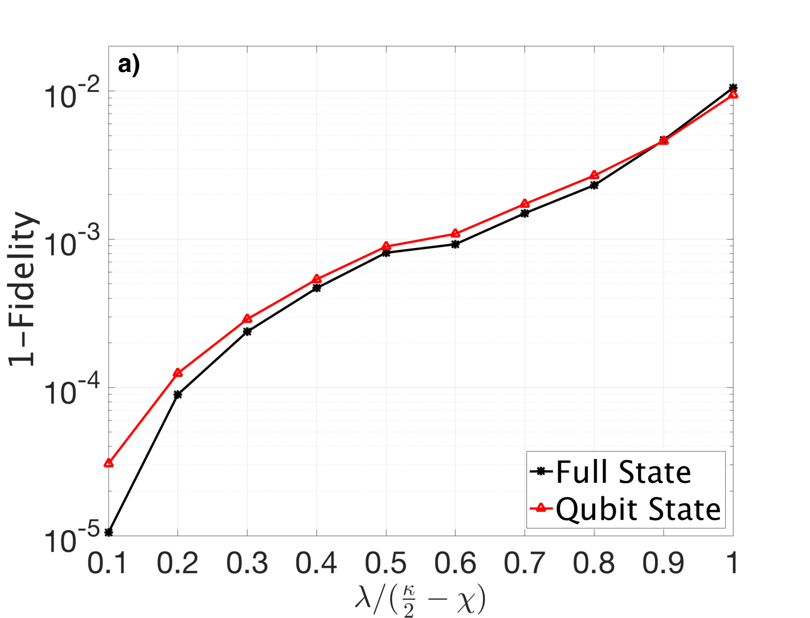
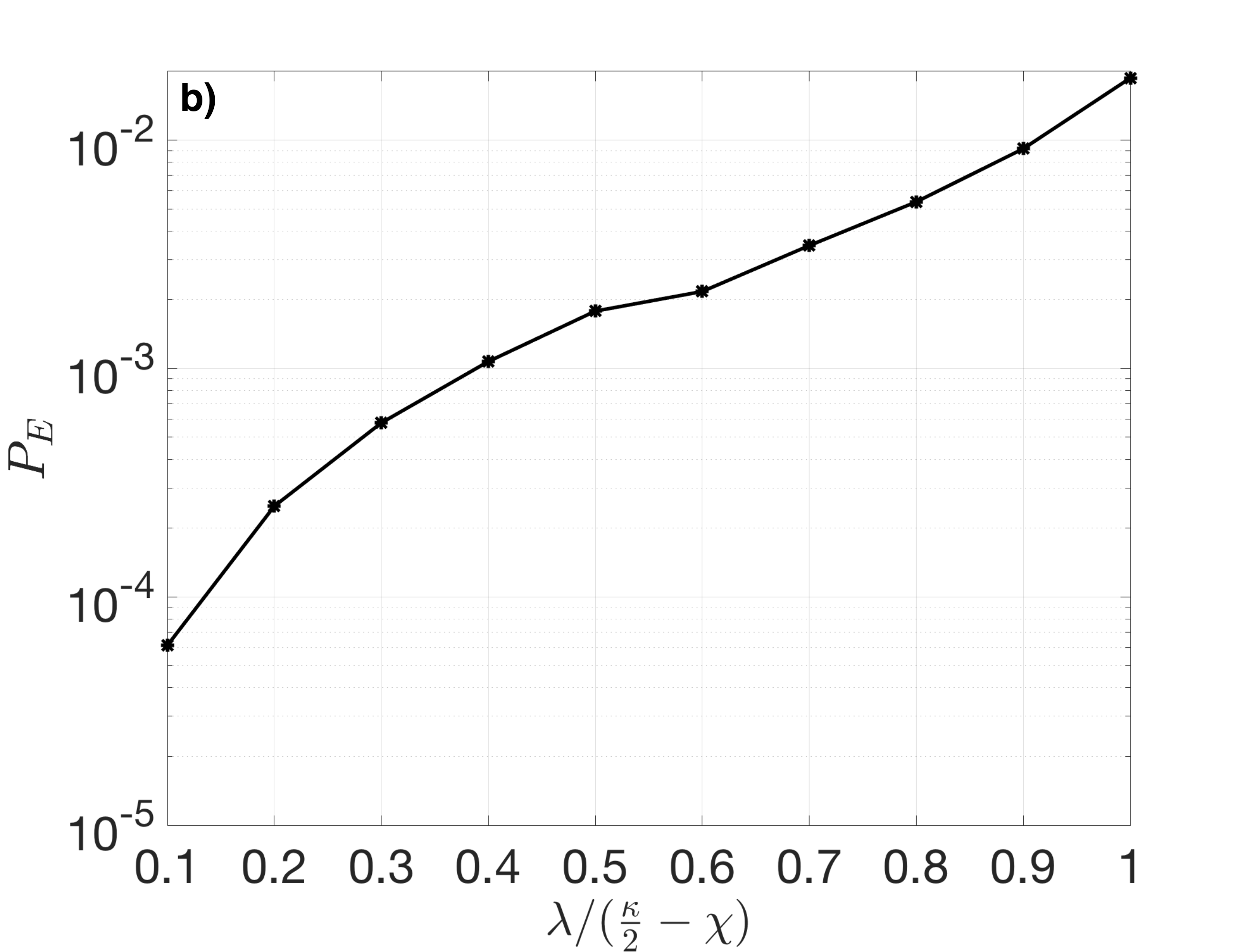
Figure 5: a) Error of the full steady-state (black stars) and qubit steady-state (red triangles) of the dispersive Hamiltonian compared to that for the full Jaynes-Cummings Hamiltonian, plotted as a function of the parametric drive strength. The system parameters are $\chi=\kappa/20$ and $\kappa=J/10$, which are well within experimental realization. b) Qubit excited state population at steady-state for the Jaynes-Cummings Hamiltonian, as a function of the parametric drive strength.

Appendix E Effect of System Losses

In this section we examine the effects of inefficiencies in transmission of the measurement signal, which we refer to as external loss, and internal loss from the cavities in the ISTMS setup. We find that both have qualitatively similar effects, and that the ISTMS setups is resilient to moderate amounts of external or internal loss.

E.1 External Loss

External loss of the signal is modeled by a beam splitter transformation on the output field $\hat{X}_{-,{\rm out}}(t)$, such that

$$\hat{X^{\prime}}_{-,{\rm out}}(t)=\sqrt{1-\eta}\hat{X}_{-,{\rm out}}(t)+\sqrt{\eta}\hat{z}_{-}(t),$$ (59)

where $\eta$ is the loss coefficient of the beam splitter, and $\hat{z}_{-}(t)$ is vacuum noise entering the signal from the other port of the beam splitter. Using this transformation, it can be shown that the signal and output noise become

$$\mathcal{M}^{\prime}_{S}(\tau)=\sqrt{1-\eta}\mathcal{M}_{S}(\tau),$$ (60)

$$\mathcal{M}^{\prime}_{N}(\tau)=(1-\eta)\mathcal{M}_{N}(\tau)+\eta\kappa\tau,$$ (61)

with $\mathcal{M}_{S}(\tau)$ and $\mathcal{M}_{N}(\tau)$ given by their expressions in C. The SNR is now given by

$${\rm SNR}^{2}_{\rm ext}=\frac{(1-\eta)\left(\mathcal{M}_{S}(\tau)\right)^{2}}{2\left[(1-\eta)\mathcal{M}_{N}(\tau)+\eta\kappa\tau\right]}.$$ (62)

In the long-time limit, and for $\lambda=\kappa/2-\chi$ this becomes

$${\rm SNR}^{2}_{\rm ext}\rightarrow\frac{4\bar{n}_{0}(1-\eta)}{1+\eta\left[\frac{1}{2}\left(\frac{\kappa}{\chi}\right)^{2}-\frac{\kappa}{\chi}\right]}\kappa\tau.$$ (63)

Therefore, for the SNR to be independent of $\chi$ in the weak coupling limit we require that

$$\frac{\chi}{\kappa}>\sqrt{\frac{\eta}{2}},$$ (64)

which restricts the amount of external loss the ISTMS setup can tolerate and still change the fundamental scaling of the SNR in the weak coupling limit.

The short time physics is also modified by external loss, and Fig. 6 shows the measurement time for different amounts of external loss. Here, the intuition from the long-time asymptotic limit also holds true, and for sufficiently small loss (in this case $1\%$) the measurement time is almost as short as for no loss. Even for $10\%$ loss the increase in measurement time is less than an order of magnitude over that for no loss.

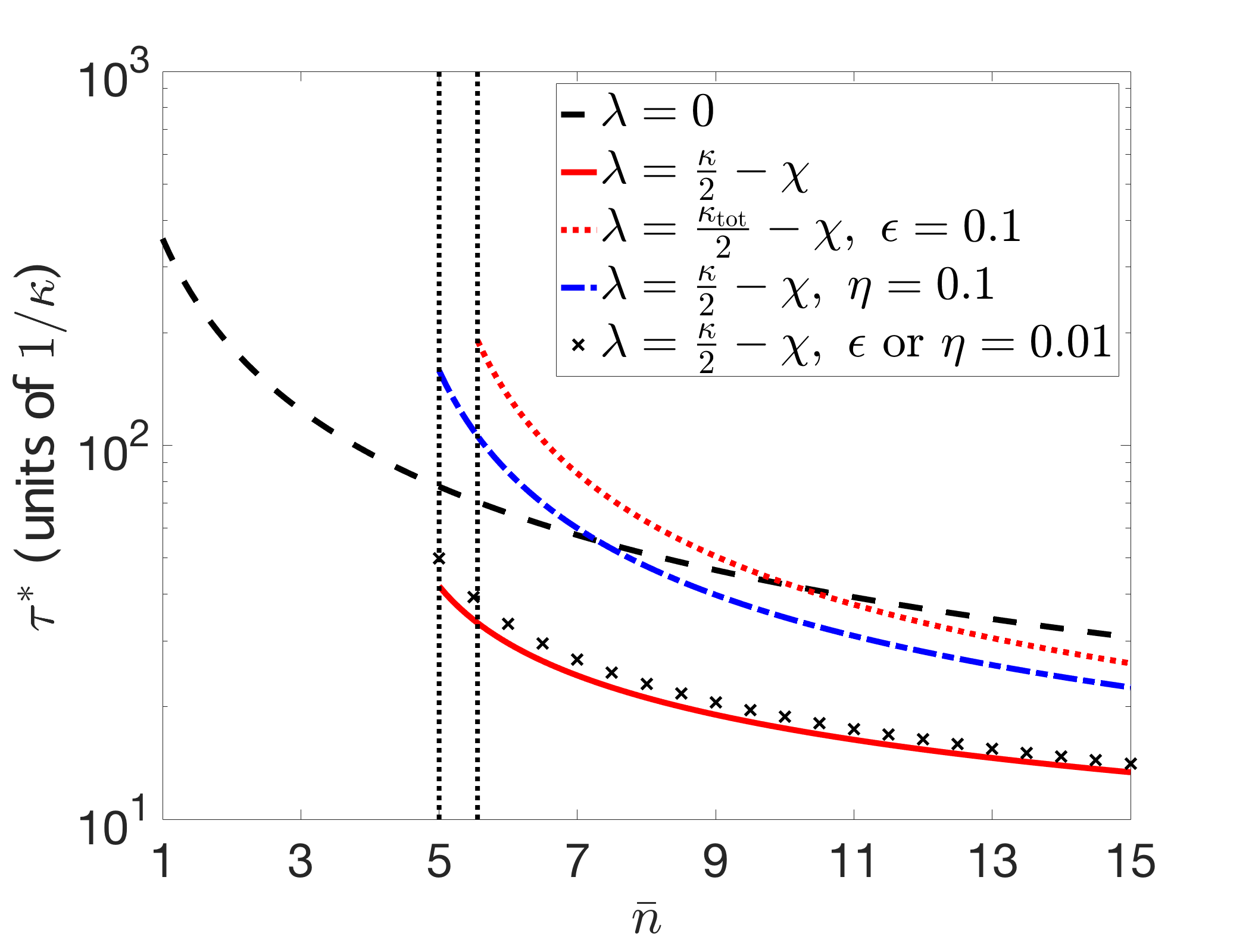
Figure 6: Weak coupling ($\chi=\kappa/20$) measurement time for various amounts of external ($\eta$) and internal ($\epsilon$) loss, as a function of total intracavity photon number $\bar{n}$. The output decay rate is $\kappa$ for all plots (i.e. $\kappa_{\rm tot}=\kappa/(1-\epsilon)$ for the internal loss plots). The dashed vertical lines indicate one plus the number of squeezed photons, with $\bar{n}_{\rm sqz}=4$ for $\epsilon=0,0.01$, and $\bar{n}_{\rm sqz}\approx 4.6$ for $\epsilon=0.1$ (the number of squeezed photons is independent of $\eta$). $\eta=\epsilon=0$ when not otherwise indicated.

E.2 Internal Loss

For internal loss we introduce the additional input-output channel $\hat{x}_{-,{\rm in/out}}(t)$ with decay rate $\kappa_{\rm int}$, which is a fraction $\epsilon$ of the total decay rate $\kappa_{\rm tot}=\kappa+\kappa_{\rm int}$, such that $\kappa_{\rm int}=\epsilon\left(\kappa+\kappa_{\rm int}\right)$. The total input state is now described by the quadrature

$$\hat{\mathcal{X}}_{-,{\rm in}}(t)=\sqrt{1-\epsilon}\hat{X}_{-,{\rm in}}(t)+\sqrt{\epsilon}\hat{x}_{-,{\rm in}}(t).$$ (65)

The input-output relation for the signal output port remains the same

$$\hat{X}_{-,{\rm out}}(t) =\hat{X}_{-,{\rm in}}(t)+\sqrt{\kappa}\hat{X}_{-}(t)$$

$$=\hat{X}_{-,{\rm in}}(t)+\sqrt{(1-\epsilon)\kappa_{\rm tot}}\hat{X}_{-}(t),$$ (66)

however, the field inside the cavities, $\hat{X}_{-}(t)$, now depends on $\hat{\mathcal{X}}_{-,{\rm in}}(t)$, not just on $\hat{X}_{-,{\rm in}}(t)$.

Following the same procedure as in C, we calculate the measurement signal and output noise, and we find that the SNR is given by the expression

$${\rm SNR}^{2}_{\rm int}=\frac{(1-\epsilon)^{2}\left(\mathcal{M}_{S}(\tau)\right)^{2}}{2\left[(1-\epsilon)\mathcal{M}_{N}(\tau)+\epsilon\kappa_{\rm tot}\tau\right]},$$ (67)

with $\mathcal{M}_{S}(\tau)$ and $\mathcal{M}_{N}(\tau)$ as before, but with $\kappa$ replaced by $\kappa_{\rm tot}$. This is qualitatively similar to the SNR for external loss, and we find that for

$$\frac{\chi}{\kappa_{\rm tot}}>\sqrt{\frac{\epsilon}{2}},$$ (68)

the SNR is independent of $\chi$ in the long-time limit for weak coupling and $\lambda=\kappa_{\rm tot}/2-\chi$. For $\epsilon\ll 1$, $\kappa_{\rm tot}\approx\kappa$ and this condition is approximately $\chi/\kappa>\sqrt{\epsilon/2}$, which is the same condition as for external loss.

For internal loss the short time physics also follows the behavior predicted by the asymptotic long-time results. As can be seen in Fig. 6, $10\%$ internal loss is slightly worse than $10\%$ external loss, but at $1\%$ loss the two situations are not discernibly different on the scale of Fig. 6 (and hence they are plotted as one curve).

Appendix F Qubit Back-Action and Purcell Decay

F.1 Density of States

To obtain the photonic density of states for the left and right cavities, we consider the system evolution in the absence of the qubit in the left/right basis

$$\dot{\hat{a}}_{R}=-iJ\hat{\sigma}_{z}\hat{a}_{L}-\kappa\hat{a}_{R}-\sqrt{2\kappa}\hat{b}_{R,{\rm in}}(t),$$ (69)

$$\dot{\hat{a}}_{L}=-i\chi\hat{\sigma}_{z}\hat{a}_{R}.$$ (70)

where we have set $\lambda=0$ for simplicity, as it does not affect the results for Purcell decay, and we are in a frame such that $\omega_{c}=\omega_{q}=0$. In frequency space, the solution to these equations is given by

$$\left(\begin{array}[]{c}\hat{a}_{R}(\omega)\\ \hat{a}_{L}(\omega)\end{array}\right)=-\sqrt{2\kappa}{\bm{\chi}}_{S}(\omega)\left(\begin{array}[]{c}\hat{b}_{R,{\rm in}}(\omega)\\ 0\end{array}\right)$$ (75)

where

$${\bm{\chi}}_{S}(\omega)=\frac{1}{i\omega(i\omega+\kappa)+J^{2}}\left(\begin{array}[]{cc}i\omega&-iJ\\ -iJ&i\omega+\kappa\end{array}\right)$$ (78)

is the susceptibility matrix for the cavities. The right and left cavity density of states are the real part of the diagonal elements of this matrix, and are given by

$$\rho[\omega]_{\rm R}=2{\rm Re}\left(\left[{\bm{\chi}}_{S}(\omega)\right]_{RR}\right)=\frac{2\kappa\omega^{2}}{\kappa^{2}\omega^{2}+\left(J^{2}-\omega^{2}\right)^{2}},$$ (79)

$$\rho[\omega]_{\rm L}=2{\rm Re}\left(\left[{\bm{\chi}}_{S}(\omega)\right]_{LL}\right)=\frac{2\kappa J^{2}}{\kappa^{2}\omega^{2}+\left(J^{2}-\omega^{2}\right)^{2}}.$$ (80)

Note that this definition is equivalent to defining the density of states in terms of the imaginary part of the retarded cavity Green’s function. The density of states is plotted in the main text, and as can be seen from the above equations, the density of states for the right resonator is zero for $\omega=0$. In the lab frame this corresponds to $\omega=\omega_{c}=\omega_{q}$, which explains the suppression of Purcell decay seen for the ISTMS setup.

F.2 Left Cavity Internal Loss

We consider internal loss in the left cavity via the system-bath Hamiltonian $\hat{H}^{\prime}_{SB}=\sqrt{2\kappa^{\prime}}\hat{B}^{{}^{\prime}\dagger}\hat{a}_{L}+h.c.$, where $\hat{B}^{{}^{\prime}\dagger}$ creates an excitation in the left cavity’s electromagnetic bath, and $\kappa^{\prime}\ll\kappa$ is the internal decay rate. Using the expressions for the eigenmodes in the dispersive regime from the main text, we see that the left cavity transforms as

$$\hat{\tilde{a}}_{L}\simeq\frac{\hat{a}_{E}-\hat{a}_{O}}{\sqrt{2}}-\frac{g}{J}\hat{\sigma}^{-},$$ (81)

In this case the two paths for the input noise from the left cavity interfere constructively, and the $\hat{\sigma}^{-}$ component remains. Therefore, Purcell decay can occur through this channel, with rate $\gamma^{\prime}_{PD}=\kappa^{\prime}\left(g/J\right)^{2}$. However, since $\kappa^{\prime}\ll\kappa$ the Purcell decay rate from the left cavity is very small, and overall, the qubit lifetime has been enhanced by the large factor $\kappa/\kappa^{\prime}$ for the ISTMS setup.

Bibliography

Bibliography

- [1] C. W. Gardiner and P. Zoller. Quantum Noise. Springer, Heidelberg, 2004.
- [2] D. F. Walls. Squeezed states of light. Nature, 306(5939):141–146, 11 1983.
- [3] Vittorio Giovannetti, Seth Lloyd, and Lorenzo Maccone. Quantum-enhanced measurements: Beating the standard quantum limit. Science, 306(5700):1330–1336, 2004.
- [4] Carlton M. Caves, Kip S. Thorne, Ronald W. P. Drever, Vernon D. Sandberg, and Mark Zimmermann. On the measurement of a weak classical force coupled to a quantum-mechanical oscillator. i. issues of principle. Rev. Mod. Phys., 52:341–392, Apr 1980.
- [5] Vladimir B. Braginsky and Farid Ya. Khalili. Quantum Measurement. Cambridge University Press, New York, NY, USA, 1992.
- [6] LIGO Scientific Collaboration. Enhanced sensitivity of the LIGO gravitational wave detector by using squeezed states of light. Nature Photonics, 7(8):613–619, jul 2013.
- [7] Kohjiro Iwasawa, Kenzo Makino, Hidehiro Yonezawa, Mankei Tsang, Aleksandar Davidovic, Elanor Huntington, and Akira Furusawa. Quantum-limited mirror-motion estimation. Phys. Rev. Lett., 111:163602, Oct 2013.
- [8] V. Peano, H. G. L. Schwefel, Ch. Marquardt, and F. Marquardt. Intracavity squeezing can enhance quantum-limited optomechanical position detection through deamplification. Phys. Rev. Lett., 115:243603, Dec 2015.
- [9] Michael A. Taylor, Jiri Janousek, Vincent Daria, Joachim Knittel, Boris Hage, BachorHans-A., and Warwick P. Bowen. Biological measurement beyond the quantum limit. Nat Photon, 7(3):229–233, 03 2013.
- [10] Sh. Barzanjeh, D. P. DiVincenzo, and B. M. Terhal. Dispersive qubit measurement by interferometry with parametric amplifiers. Physical Review B, 90(13):134515, oct 2014.
- [11] Nicolas Didier, Archana Kamal, William D Oliver, Alexandre Blais, and Aashish A Clerk. Heisenberg-Limited Qubit Read-Out with Two-Mode Squeezed Light. Phys. Rev. Lett., 115(9):093604, aug 2015.
- [12] Jerry M. Chow, Jay M. Gambetta, Easwar Magesan, David W. Abraham, Andrew W. Cross, B R Johnson, Nicholas A. Masluk, Colm A. Ryan, John A. Smolin, Srikanth J. Srinivasan, and M Steffen. Implementing a strand of a scalable fault-tolerant quantum computing fabric. Nat Commun, 5:4015, 06 2014.
- [13] M. Hatridge, S. Shankar, M. Mirrahimi, F. Schackert, K. Geerlings, T. Brecht, K. M. Sliwa, B. Abdo, L. Frunzio, S. M. Girvin, R. J. Schoelkopf, and M. H. Devoret. Quantum back-action of an individual variable-strength measurement. Science, 339(6116):178–181, 2013.
- [14] Evan Jeffrey, Daniel Sank, J. Y. Mutus, T. C. White, J. Kelly, R. Barends, Y. Chen, Z. Chen, B. Chiaro, A. Dunsworth, A. Megrant, P. J. J. O’Malley, C. Neill, P. Roushan, A. Vainsencher, J. Wenner, A. N. Cleland, and John M. Martinis. Fast accurate state measurement with superconducting qubits. Phys. Rev. Lett., 112:190504, May 2014.
- [15] K. W. Murch, S. J. Weber, C. Macklin, and I. Siddiqi. Observing single quantum trajectories of a superconducting quantum bit. Nature, 502(7470):211–214, 10 2013.
- [16] D Ristè, M Dukalski, C A Watson, G de Lange, M J Tiggelman, Ya M Blanter, K W Lehnert, R N Schouten, and L DiCarlo. Deterministic entanglement of superconducting qubits by parity measurement and feedback. Nature, 502(7471):350–4, October 2013.
- [17] N. Roch, M. E. Schwartz, F. Motzoi, C. Macklin, R. Vijay, A. W. Eddins, A. N. Korotkov, K. B. Whaley, M. Sarovar, and I. Siddiqi. Observation of measurement-induced entanglement and quantum trajectories of remote superconducting qubits. Phys. Rev. Lett., 112:170501, Apr 2014.
- [18] L Steffen, Y Salathe, M Oppliger, P Kurpiers, M Baur, C Lang, C Eichler, G Puebla-Hellmann, A Fedorov, and A Wallraff. Deterministic quantum teleportation with feed-forward in a solid state system. Nature, 500(7462):319–22, August 2013.
- [19] C. Eichler, D. Bozyigit, C. Lang, M. Baur, L. Steffen, J. M. Fink, S. Filipp, and A. Wallraff. Observation of two-mode squeezing in the microwave frequency domain. Phys. Rev. Lett., 107:113601, Sep 2011.
- [20] L Zhong, E P Menzel, R Di Candia, P Eder, M Ihmig, A Baust, M Haeberlein, E Hoffmann, K Inomata, T Yamamoto, Y Nakamura, E Solano, F Deppe, A Marx, and R Gross. Squeezing with a flux-driven josephson parametric amplifier. New Journal of Physics, 15(12):125013, 2013.
- [21] C. Eichler, Y. Salathe, J. Mlynek, S. Schmidt, and A. Wallraff. Quantum-limited amplification and entanglement in coupled nonlinear resonators. Phys. Rev. Lett., 113:110502, Sep 2014.
- [22] K. W. Murch, S. J. Weber, K. M. Beck, E. Ginossar, and I. Siddiqi. Reduction of the radiative decay of atomic coherence in squeezed vacuum. Nature, 499(7456):62–65, 07 2013.
- [23] D. M. Toyli, A. W. Eddins, S. Boutin, S. Puri, D. Hover, V. Bolkhovsky, W. D. Oliver, and I. Siddiqi. Resonance fluorescence from an artificial atom in squeezed vacuum. Phys. Rev. X 6, 031004 (2016), 2016.
- [24] Nicolas Didier, Jérôme Bourassa, and Alexandre Blais. Fast quantum nondemolition readout by parametric modulation of longitudinal qubit-oscillator interaction. Phys. Rev. Lett., 115:203601, Nov 2015.
- [25] K D Petersson, L W McFaul, M D Schroer, M Jung, J M Taylor, A A Houck, and J R Petta. Circuit quantum electrodynamics with a spin qubit. Nature, 490(7420):380–3, oct 2012.
- [26] J J Viennot, M C Dartiailh, A Cottet, and T Kontos. Coherent coupling of a single spin to microwave cavity photons. Science (New York, N.Y.), 349(6246):408–11, jul 2015.
- [27] A Stockklauser, V F Maisi, J Basset, K Cujia, C Reichl, W Wegscheider, T Ihn, A Wallraff, and K Ensslin. Microwave Emission from Hybridized States in a Semiconductor Charge Qubit. Physical review letters, 115(4):046802, jul 2015.
- [28] Gengyan Zhang, Yanbing Liu, James J. Raftery, and Andrew A. Houck. Suppression of photon shot noise dephasing in a tunable coupling superconducting qubit. mar 2016.
- [29] T. Yamamoto, K. Inomata, M. Watanabe, K. Matsuba, T. Miyazaki, W. D. Oliver, Y. Nakamura, and J. S. Tsai. Flux-driven josephson parametric amplifier. Applied Physics Letters, 93(4), 2008.
- [30] Christopher Eichler and Andreas Wallraff. Controlling the dynamic range of a josephson parametric amplifier. EPJ Quantum Technology, 1(1):2, 2014.
- [31] Mankei Tsang and Carlton M. Caves. Evading quantum mechanics: Engineering a classical subsystem within a quantum environment. Phys. Rev. X, 2:031016, Sep 2012.
- [32] A. A. Clerk, M. H. Devoret, S. M. Girvin, Florian Marquardt, and R. J. Schoelkopf. Introduction to quantum noise, measurement, and amplification. Rev. Mod. Phys., 82:1155–1208, Apr 2010.
- [33] Alexandre Blais, Ren-Shou Huang, Andreas Wallraff, S. Girvin, and R. Schoelkopf. Cavity quantum electrodynamics for superconducting electrical circuits: An architecture for quantum computation. Physical Review A, 69(6):062320, jun 2004.
- [34] Mostafa Khezri, Eric Mlinar, Justin Dressel, and Alexander N. Korotkov. Measuring a transmon qubit in circuit qed: Dressed squeezed states. Phys. Rev. A, 94:012347, Jul 2016.
- [35] Daniel Sank, Zijun Chen, Mostafa Khezri, J. Kelly, R. Barends, B. Campbell, Y. Chen, B. Chiaro, A. Dunsworth, A. Fowler, E. Jeffrey, E. Lucero, A. Megrant, J. Mutus, M. Neeley, C. Neill, P. J. J. O’Malley, C. Quintana, P. Roushan, A. Vainsencher, T. White, J. Wenner, Alexander N. Korotkov, and John M. Martinis. Measurement-induced state transitions in a superconducting qubit: Beyond the rotating wave approximation. Phys. Rev. Lett., 117:190503, Nov 2016.
- [36] M. D. Reed, B. R. Johnson, A. A. Houck, L. DiCarlo, J. M. Chow, D. I. Schuster, L. Frunzio, and R. J. Schoelkopf. Fast reset and suppressing spontaneous emission of a superconducting qubit. Applied Physics Letters, 96(20):203110, may 2010.
- [37] Luke C. G. Govia and Frank K. Wilhelm. Unitary-feedback-improved qubit initialization in the dispersive regime. Phys. Rev. Applied, 4:054001, Nov 2015.
- [38] N. T. Bronn, E. Magesan, N. A. Masluk, J. M. Chow, J. M. Gambetta, and M. Steffen. Reducing spontaneous emission in circuit quantum electrodynamics by a combined readout/filter technique. IEEE Transactions on Applied Superconductivity, 25(5):1–10, Oct 2015.
- [39] M. I. Dykman, M. Marthaler, and V. Peano. Quantum heating of a parametrically modulated oscillator: Spectral signatures. Phys. Rev. A, 83:052115, May 2011.
- [40] M. Marthaler and M. I. Dykman. Switching via quantum activation: A parametrically modulated oscillator. Phys. Rev. A, 73:042108, Apr 2006.
- [41] N Bergeal, R Vijay, V E Manucharyan, I Siddiqi, R J Schoelkopf, S M Girvin, and M H Devoret. Analog information processing at the quantum limit with a Josephson ring modulator. Nat Phys, 6(4):296–302, apr 2010.
- [42] N Bergeal, F Schackert, M Metcalfe, R Vijay, V E Manucharyan, L Frunzio, D E Prober, R J Schoelkopf, S M Girvin, and M H Devoret. Phase-preserving amplification near the quantum limit with a Josephson ring modulator. Nature, 465(7294):64–68, may 2010.
- [43] K. M. Sliwa, M. Hatridge, A. Narla, S. Shankar, L. Frunzio, R. J. Schoelkopf, and M. H. Devoret. Reconfigurable josephson circulator/directional amplifier. Phys. Rev. X, 5:041020, Nov 2015.
- [44] Luke C. G. Govia and Frank K. Wilhelm. Entanglement generated by the dispersive interaction: The dressed coherent state. Phys. Rev. A, 93:012316, Jan 2016.
- [45] Matthew Elliott and Eran Ginossar. Enhancement and state tomography of a squeezed vacuum with circuit quantum electrodynamics. Phys. Rev. A, 92:013826, Jul 2015.