Kondo temperature when the Fermi level is near a step in the conduction density of states

Abstract

The (111) surface of Cu, Ag and Au is characterized by a band of surface Shockley states, with constant density of states beginning slightly below the Fermi energy. These states as well as bulk states hybridize with magnetic impurities which can be placed above the surface. We calculate the characteristic low-temperature energy scale, the Kondo temperature $T_{K}$ of the impurity Anderson model, as the bottom of the conduction band $D_{s}$ crosses the Fermi energy $\epsilon_{F}$. We find simple power laws $T_{K}\simeq|D_{s}-\epsilon_{F}|^{\eta}$, where $\eta$ depends on the sign of $D_{s}-\epsilon_{F}$, the ratio between surface and bulk hybridizations with the impurity $\Delta_{s}/\Delta_{b}$ and the ratio between on-site and Coulomb energy $E_{d}/U$ in the model.

I Introduction

The Kondo effect is one of the paradigmatic phenomena in strongly correlated condensed matter systems hewson . It takes place when a localized magnetic impurity interacts via an exchange interaction with extended states. Below a characteristic temperature $T_{K}$, the impurity spin is screened by the conduction electrons, and the ground state is a many-body singlet formed by the impurity spin and the spin of the conduction electrons. Originally observed in dilute magnetic alloys, the Kondo effect has reappeared more recently in the context of semiconducting gold ; cro ; wiel ; grobis ; ama and molecular liang ; kuba ; parks ; roch ; parks2 ; serge ; vincent quantum-dot systems, and in systems of magnetic adatoms (e.g., Co or Mn) deposited on clean metallic surfaces, where the effect has been clearly observed experimentally as a narrow Fano-Kondo antiresonance in the differential conductance ($G(V)=dI/dV$, where $I$ is the current and $V$ the applied voltage) observed by a scanning tunneling microscope (STM) li ; madha ; man ; knorr ; limot ; henzl ; serra .

A STM permits the manipulation of single atoms or molecules on top of a surface eigler and the construction of structures of arbitrary shape such as quantum corrals.crom ; heller ; man The differential conductance measured by the STM is in general proportional to the local density of metal states, and it has contributions from bulk and surface states.fiete ; revi These contributions are weighted differently by the STM tip due to the different decay rate of the wave functions out of the surface.plihal The effect of the different distance dependence of tunneling processes involving $3d$ and $s/p$ states has been observed recently for Fe₂N on Cu(001).taka

The (111) surfaces of Cu, Ag and Au were used as the substrate for many observations of the Kondo effect li ; madha ; man ; knorr ; limot ; henzl ; serra ; zhao ; kome ; mina ; iancu and have the property that a parabolic band of two-dimensional Shockley surface states, confined to the last few atomic planes exists.hulb ; cerce ; abd This band is uncoupled to bulk states for small wave vectors parallel to the surface, due to the presence of a bulk-projected band gap at the center of the surface Brillouin zone.hulb These surface states represent an almost ideal example of a two-dimensional electron gas on a metal surface. The effective mass is between 0.31 and 0.38 of the electron mass,crom ; euc ; limot and the constant surface density of states begins at a step which lies below the Fermi energy by an energy $\approx 450$ meV for Cu,knorr $\approx 475$ meV for Au,cerce and $\approx 67$ meV for Ag.limot The corresponding steps have been observed in STM experiments.cerce ; limot Interestingly, it has been shown recently that the Shockley surface states can be thought as topologically derived surface states from a topological energy gap lying about $\sim$ 3 eV above the Fermi energy.claudia

The surface states are expected to be more sensitive to adatoms at the surface, and this fact has been used to confine electrons in corrals or resonators built from different adatoms.heller Recently, it has been shown that the effect on the surface density of states of resonators of Co and Ag adatoms built on the Ag(111) observed by an STM can be modeled by the effect of an attractive potential at the position of the adatoms on free electrons in two dimensions.joaq In a famous experiment, a Co atom acting as a magnetic impurity was placed at one focus of an elliptical quantum corral built on the Cu(111) surface. A Fano-Kondo antiresonance was observed in the differential conductance not only at that position, but also with reduced intensity at the other focus.man This “mirage” can be understood as the result of quantum interference in the way in which the Kondo effect is transmitted from one focus to the other by the different eigenstates of surface conduction electrons inside a hard-wall ellipse.revi ; rap ; por ; wei ; hal ; ali2 ; wil This experiment reveals that conducting surface states have an important hybridization with the impurity, although other experiments suggests that the hybridization of bulk electrons plays the dominant role in this effect. knorr ; limot ; henzl Interestingly, a Kondo resonance with $T_{K}\sim 180$ K was obtained for a system of a molecule containing a magnetic Co atom on a Si substrate prepared in such a way to have a surface metallic state on top of insulating Si.li2 In this case clearly bulk states do not contribute to the observed Kondo resonance. Some calculations suggest that surface states give an important contribution to the Fano-Kondo antiresonance,merino while others obtain a contribution of 1/36 or less depending on the orbital.barral A recent study for Co on Cu(111) suggests that the line shape of the Kondo resonance is affected by the presence of surface states.Baruselli From the mirage intensity it has been estimated that the coupling to the surface states is at least 1/10 that of the bulk.revi Recent experiments for a Co impurity on Ag(111) moro in which the surface density of states at the Fermi level $\rho_{s}(0)$ has been modified by means of resonators moro ; joaq obtain an increase of a factor larger than 2 in $T_{K}$ as a consequence of a moderate increase in $\rho_{s}(0)$, indicating a very important contribution of the surface states to the Kondo effect.

As we show in the next section, for hybridization independent of the energy (as usually assumed to be a reasonable approximation), the presence of a step in the conduction spectral density near the Fermi energy has dramatic effects on the Kondo temperature $T_{K}$ (the characteristic energy scale of the Kondo effect). It has been shown that the bottom of the surface band $D_{s}$ can be changed by alloying the different noble metals at the surface.cerce ; abd In fact this displacement has been measured by STM,cerce and it should be possible to use the STM to measure also the Fano-Kondo antiresonance and determine $T_{K}$. One may suspect that disorder affects the sharp onset of the surface states at $D_{s}$ but the states at this onset have very long wave length averaging the disorder. Furthermore, experiments on epitaxial Ag(111) films on Si(111)-($7\times 7$) have shown that it is possible to change $D_{s}$ and make it cross the Fermi energy by strain.neu We note that recent developments in scientific instruments using a piezoelectric vice,andy1 have been used to obtain both uniaxial compression and uniaxial tension on different samples. As an example, both effects increase the superconducting critical temperature of Sr₂RuO₄.andy2

In this work we calculate the Kondo temperature as a function of the bottom of the surface band, using different techniques: poor man’s scaling (PMS)hewson ; and on the effective Kondo model, non-crossing approximation (NCA),hewson ; bickers , slave bosons in the mean-field approximation (SBMFA),hewson ; cole ; newns and numerical-renormalization group (NRG).hewson ; Bulla ; Wilson ; Cragg ; Krishna ; Campo These approaches are known to reproduce correctly the relevant energy scale $T_{K}$ and its dependence of parameters in cases in which the conduction density of states is smooth. As we shall see, the presence of the surface states introduces some complications, due to the divergence of the one-body part of the self energy [Eq. (6) below] at energies near the step, but this can be handled by the NCA, which exactly incorporates arbitrary conduction densities and hybridizations in its integral equations.kroha

The PMS is a perturbative approach that integrates out progressively a small portion of the conduction states lying at the bottom and at the top of the conduction bands, renormalizing the Kondo coupling $J$. It ceases to be valid when $|D_{s}-\epsilon_{F}|\sim J$, where $\epsilon_{F}$ is the Fermi energy.hewson ; and

The NCA is equivalent to a sum of an infinite series of diagrams in perturbations in the hybridization.hewson ; bickers In contrast to NRG in which finite-energy features are artificially broadened due to the logarithmic discretization of the conducting band zitko ; loig , NCA correctly describes these features. For instance, the intensity and the width of the charge-transfer peak of the spectral density (the one near the dot level $E_{d}$) was found capa in agreement with other theoretical methods pru ; logan and experiment haug . Furthermore, it has a natural extension to non-equilibrium conditions wingreen and it is specially suitable for describing satellite peaks of the Kondo resonance, as those observed in Ce systems,reinert ; ehm or away from zero bias voltage in non-equilibrium transport.tosi_2 ; NFL ; st An alternative to NCA for non-equilibrium problems is renormalized perturbation theory, but it is limited to small bias voltage.hbo ; ng

The SBMFA, as the NCA uses a pseudoparticle representation, but in contrast to the latter, neglects the dynamics of the pseudoboson and takes it in average.hewson ; cole ; newns In spite of this and the fact that the charge-transfer peak is lost, the spectral density near the Fermi level and low-energy properties are well described. For this reason it has been successful in describing several Kondo systems,rome ; si ; mole including adatoms or molecules on the (111) surface of Cu or noble metals.revi ; rome ; mole ; joa2

The NRG is a very accurate technique that has been used for many problems. Baruselli ; Bulla ; Wilson ; Cragg ; Krishna ; Campo However, as stated above, in some cases it misses some finite energy features. This fact seems to introduce some difficulties in our problem, as we shall show.

In Sec. II, we describe the impurity Anderson model, the particularities of our case, and its Kondo limit used in PMS. The results are presented in Sec. III and Sec. IV contains a summary and discussion.

II Model and formalism

II.1 Hamiltonian

The Hamiltonian can be written as

$$H = \sum_{k\sigma}\varepsilon_{k}^{s}s_{k\sigma}^{\dagger}s_{k\sigma}+\sum_{k\sigma}\varepsilon_{k}^{b}b_{k\sigma}^{\dagger}b_{k\sigma}+E_{d}\sum_{\sigma}d_{\sigma}^{\dagger}d_{\sigma}+$$ (1)

$$+U\sum d_{\uparrow}^{\dagger}d_{\uparrow}d_{\downarrow}^{\dagger}d_{\downarrow}+\sum_{k\sigma}V_{k}^{s}[d_{\sigma}^{\dagger}s_{k\sigma}+\text{H.c.}]+$$

$$+\sum_{k\sigma}V_{k}^{b}[d_{\sigma}^{\dagger}b_{k\sigma}+\text{H.c.}].$$

where $d_{\sigma}^{\dagger}$ creates an electron with spin $\sigma$ at the relevant orbital of the magnetic impurity (assumed non-degenerate) and $s_{k\sigma}^{\dagger}$ ($b_{k\sigma}^{\dagger}$) are creation operators for an electron in the $k^{th}$ surface (bulk) conduction eigenstate.

The spectral density of electrons at the magnetic impurity is

$$\rho_{d\sigma}(\omega)=\frac{1}{2\pi i}[G_{d\sigma}(\omega-i\epsilon)-G_{d\sigma}(\omega+i\epsilon)],$$ (2)

where $\epsilon$ is a positive infinitesimal. Calling $z=\omega+i\epsilon$ ($z=\omega-i\epsilon$), the retarded (advanced) Green’s function at the interacting QD can be written in the form lan ; mir

$$G_{d\sigma}(z)=\frac{1}{z-E_{d}-\Sigma_{0\sigma}(z)-\Sigma_{d\sigma}(z)},$$ (3)

where $\Sigma_{d\sigma}(z)$ is the self-energy due to the interaction $U$ and $\Sigma_{0}(z)$, the non-interacting part of the self-energy (present also for $U=0$) is

$$\Sigma_{0\sigma}(z) = \Sigma_{0\sigma}^{b}(z)+\Sigma_{0\sigma}^{s}(z),$$

$$\Sigma_{0\sigma}^{c}(z) = \sum_{k}\frac{|V_{k}^{c}|^{2}}{z-\varepsilon_{k}^{c}},$$ (4)

where $c=b$ or $c=s$. As usual in this type of problems, in which the bulk contribution has no special features near the Fermi level, we assume a constant density of bulk states $\rho_{b}$ extending in a wide range from $-D$ to $D$, and a constant hybridization $V_{k}^{b}$. Defining $\Delta_{b}=\pi\rho_{b}|V_{k}^{b}|^{2}$, for energies near the Fermi level $\epsilon_{F}$ ($D\gg|\omega-\epsilon_{F}|$), we can neglect the real part of the bulk contribution to $\Sigma_{0\sigma}(z)$ revi and it becomes simply

$$\Sigma_{0\sigma}^{b}(\omega+i\epsilon)=-i\Delta_{b}.$$ (5)

The surface contribution do the density of states $\rho_{s}$ is constant and begins near the Fermi energy at $D_{s}$. For simplicity we assume that it ends also at $D$ as the bulk one. Then

$$\Sigma_{0\sigma}^{s}(\omega+i\epsilon)=-\frac{\Delta_{s}}{\pi}\ln\left(\frac{D-\omega}{|D_{s}-\omega|}\right)-i\Delta_{s}\theta(\omega-D_{s}),$$ (6)

where $\Delta_{s}=\pi\rho_{s}|V_{k}^{s}|^{2}$ and $\theta(\omega)$ is the step function. Thus, the non-interacting ($U=0$) Green’s function can be written in the form

$$G_{d\sigma}^{0}(z)=\frac{1}{z-\tilde{E}_{d}(\omega)+i[\Delta_{b}+\Delta_{s}\theta(\omega-D_{s})]},$$ (7)

where

$$\tilde{E}_{d}(\omega)=E_{d}-\frac{\Delta_{s}}{\pi}\ln\left(\frac{D-\omega}{|D_{s}-\omega|}\right)$$ (8)

is an effective energy of the localized level.

II.2 The Kondo limit

The Kondo effect takes place for dot occupations near one. This condition in terms of the parameters means $\Delta_{b}+\Delta_{s}\theta(\epsilon_{F}-D_{s})\ll\epsilon_{F}-\tilde{E}_{d}(\epsilon_{F})$, $\tilde{E}_{d}(\epsilon_{F})+U-\epsilon_{F}$. The Kondo Hamiltonian is obtained from the Anderson one by means of a canonical transformation to second order in the hybridization $V_{k}^{b}$ and $V_{k}^{s}$.hewson ; sw To simplify the problem, using the fact that all physical quantities depend on conduction spectral densities and hybridization only through the products $\Delta_{b}$ and $\Delta_{s}$, we consider an equivalent problem in which both hybridizations are equal to the bulk one and the new surface density of states $\tilde{\rho}_{s}$ is modified accordingly in such a way that

$$\Delta_{s}=\pi\tilde{\rho}_{s}|V_{k}^{b}|^{2}.$$ (9)

Then, the effective Kondo interaction can be written in the form

$$H_{K}=J\sum\limits_{kq}[S^{+}c_{k\downarrow}^{\dagger}c_{q\uparrow}+S^{-}c_{k\uparrow}^{\dagger}c_{q\downarrow}+S_{z}(c_{k\uparrow}^{\dagger}c_{q\uparrow}-c_{k\downarrow}^{\dagger}c_{q\downarrow})],$$ (10)

where $c_{i\sigma}^{\dagger}$ ($i=k,q$) includes both, bulk and surface conduction electrons, and the spin operators act on the localized spin ($|\sigma\rangle=d_{\sigma}^{\dagger}|0\rangle$). The interaction is calculated for conduction states near the Fermi energy $\epsilon_{F}$ and becomes for $V_{k}^{b}=V$ near $\epsilon_{F}$

$$J=\frac{|V|^{2}}{\epsilon_{F}-\tilde{E}_{d}(\epsilon_{F})}+\frac{|V|^{2}}{\tilde{E}_{d}(\epsilon_{F})+U-\epsilon_{F}}.$$ (11)

III Results

In this section we present the results of the different techniques used. For simplicity, from now on we choose the origin of energies at $\epsilon_{F}=0$.

III.1 Poor man’s scaling

Here used the PMS hewson ; and for the Kondo Hamiltonian, which allows us to obtain analytical results in the Kondo regime and for $|D_{s}|\gtrsim J$. The idea is very simple. Integrating out successively the states on the top and bottom of the conduction band renormalizing $J$, one has the same problem but with a smaller total band width (from $-D^{\prime}$ to $D^{\prime}$ and larger Kondo interaction $J(D^{\prime})$. Proceeding in this way until $D^{\prime}=|D_{s}|$, the step in the density of states disappears and one recovers the ordinary Kondo problem. In its simplest form (to second order in $J$), the equation for the change in $J$ in the range where the running cutoff $D^{\prime}$ is larger than $|D_{s}|$ is

$$\frac{dJ}{d\ln D^{\prime}}=-(2\rho_{b}+\tilde{\rho}_{s})J^{2}.$$ (12)

The different factors in front of the densities is due to the fact that the surface part only acts at the top of the band.

Integrating Eq. (12) one has an equation for $J(|D_{s}|)$

$$D\exp\left[-\frac{1}{(2\rho_{b}+\tilde{\rho}_{s})J}\right]=|D_{s}|\exp\left[-\frac{1}{(2\rho_{b}+\tilde{\rho}_{s})J(|D_{s}|)}\right],$$ (13)

and now one can use the expression for the Kondo temperature for a band with $|D_{s}|$, Kondo interaction $J(|D_{s}|)$ and density $\rho=\rho_{b}+\tilde{\rho}_{s}$ ($\rho=\rho_{b}$) for $D_{s}<0$ ($D_{s}>0$):

$$T_{K}\simeq|D_{s}|\exp\left[-\frac{1}{2\rho J(|D_{s}|)}\right].$$ (14)

Using Eqs. (9), (13) and (14) one obtains for $D_{s}<0$

$$T_{K} \simeq |D_{s}|^{\nu}D^{1-\nu}\exp\left[-\frac{1}{2J(\rho_{b}+\tilde{\rho}_{s})}\right],$$

$$\nu = \frac{\Delta_{s}}{2(\Delta_{b}+\Delta_{s})},$$ (15)

and for $D_{s}>0$

$$T_{K} \simeq D_{s}^{-\mu}D^{1+\mu}\exp\left[-\frac{1}{2J\rho_{b}}\right],$$

$$\mu = \frac{\Delta_{s}}{2\Delta_{b}}.$$ (16)

From Eqs. (8) and (11) one has

$$\frac{1}{J\rho_{b}} = \frac{\pi}{\Delta_{b}U}[-E_{d}(E_{d}+U)-(2E_{d}+U)x-x^{2}],$$

$$x = \frac{\Delta_{s}}{\pi}\ln\frac{|D_{s}|}{D}.$$ (17)

If $|D_{s}|$ is not too small, one can neglect the term in $x^{2}$ in comparison with the first term in square brackets in Eq. (17). In any case for small $|D_{s}|$, the PMS ceases to be valid. Using this approximation and replacing Eq. (17) in Eqs. (15) and (16) we obtain

$$T_{K} \simeq A|D_{s}|^{\eta}D^{1-\eta}\exp\left[\frac{\pi E_{d}(E_{d}+U)}{2U(\Delta_{b}+\Delta_{s})}\right],$$

$$\eta = \frac{\Delta_{s}}{(\Delta_{b}+\Delta_{s})}(1+\frac{E_{d}}{U}),\text{ if }D_{s}<0.$$

$$T_{K} \simeq BD_{s}^{\zeta}D^{1-\zeta}\exp\left[\frac{\pi E_{d}(E_{d}+U)}{2U\Delta_{b}}\right],$$

$$\zeta = \frac{\Delta_{s}E_{d}}{\Delta_{b}U},\text{ if }D_{s}>0,$$ (18)

where to second order in $J$, $A=B=1$. This is the main result of this section. As expected, the expressions are correct in the obvious limits, $\Delta_{s}=0$, $D_{s}=-D$, and $D_{s}=D$, although the prefactor is somewhat larger that a more accurate one that can be obtained including terms up to third order in $J$ in PMS.hewson ; solyom Including these terms in the present case is more involved than in the usual case in which an electron-hole symmetric conduction band is assumed. Terms of order $J^{3}/(D^{\prime}+|D_{s}|)$ appear when calculating $dJ/dD^{\prime}$ and an analytical solution of the differential equation is not possible. When $|D_{s}|=D$, the band recovers the electron-hole symmetry and we can borrow previous results, that we display for later use:

$$A = \sqrt{2\rho_{b}J(1+\Delta_{s}/\Delta_{b})},$$

$$B = \sqrt{2\rho_{b}J},$$ (19)

where $\rho_{b}J$ is given by Eq. (17).

For comparison with the results of other techniques, we note the limiting values of the exponents for infinite $U$ depending if either $E_{d}$ or $E_{d}+U$ remains finite

$$\eta = \frac{\Delta_{s}}{(\Delta_{b}+\Delta_{s})}\text{, }\zeta=0$$

$$\text{if }U \rightarrow +\infty,E_{d}\text{ finite,}$$ (20)

$$\eta = 0\text{, }\zeta=-\frac{\Delta_{s}}{\Delta_{b}}$$

$$\text{if }U \rightarrow +\infty,E_{d}+U\text{ finite.}$$ (21)

III.2 Non-crossing and slave-boson mean-field approximations

The non-crossing approximation (NCA) is a diagrammatic technique that reproduces correctly the Kondo temperature of the spin-1/2 impurity Anderson model in the limit $U\rightarrow+\infty$.hewson ; bickers Unfortunately, this is not the case for finite $U$ pruschke89 ; haule01 ; tosi11 . Therefore, we restrict the NCA calculations to $U\rightarrow+\infty$. To determine the value of the Kondo temperature $T_{K}$, we calculate the conductance through the magnetic impurity as a function of temperature $G(T)$ and look for the temperature such that $G(T_{K})=G_{0}/2$, where $G_{0}$ is the ideal conductance of the system (reached for $T=0$ and occupancy 1 of the dot level). Alternative definitions of $T_{K}$ differ in factor of the order of 1,tositk which is not relevant to us, since we are interested in the dependence of $T_{K}$ with $D_{s}$.

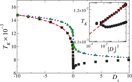
Figure 1: (Color online) Kondo temperature as a function of the bottom of the conduction band. Squares and circles: NCA. Triangles: SBMFA. Dashed (dot) line: fit to the NCA (SBMFA) results. The inset shows the NCA results in log-log scale. Parameters are $E_{d}=-4$, $\Delta_{b}=1$, $\Delta_{s}=0.1$.

In the following we take $\Delta_{b}+\Delta_{s}$ of the order of the unit of energy and set $D=10$. We begin taking $E_{d}=-4$ so that the system is in the Kondo regime. In Fig. 1 we show the resulting $T_{K}$ as a function of $D_{s}$ for a ratio $\Delta_{s}/\Delta_{b}=1/10$, the lower limit estimated on the basis of the mirage experiment for a Co impurity inside an elliptical corral on the Cu(111) surface.revi A fit of the NCA results with the function $T_{K}=C|D_{s}|^{\eta}$ in the interval $-10\leq D_{s}\leq-0.5$ gives $C=0.01204$ and $\eta=0.09039$. The exponent is in very good agreement with the PMS result $\eta=1/11=0.09091$ from Eq. (20). For smaller $|D_{s}|$, in particular when $|D_{s}|\sim T_{K}$, the PMS ceases to be valid. The NCA gives a continuous function for $T_{K}$ with a finite value for $D_{s}=0$. For positive $D_{s}$, PMS predicts a constant $T_{K}$ [Eqs. (18) and (20)]. As a first approximation, the NCA results are consistent with this. However, for small $D_{s}$, $T_{K}$ decreases by about 17%. There is also a non-monotonic behavior with a minimum near $D_{s}=0$. Concerning the magnitude of $T_{K}$, the NCA value for $D_{s}=-D$ is 0.0148, while Eq. (18) with $A=0.42$ given by Eq. (19) gives $T_{K}=0.0139$ in good agreement with the NCA result. For $D_{s}=D$, the corresponding values are 0.0080 and 0.0075 respectively. The NCA values are near 7% higher.

In Fig. 1 we also show the result of $T_{K}$ using the SBMFA for the same parameters. In this case, we define $T_{K}$ as the half width at half maximum of the Kondo resonance in the spectral density of states. The results shown in the figure were multiplied by 0.447 so that they coincide with those of the NCA for $D_{s}=-D$. Curiously, this factor is similar to $A=0.42$ discussed above. Although the SBMFA gives the correct order of magnitude of $T_{K}$ for not too small $D_{s}$, the dependence with $D_{s}$ is not reproduced, although the function can still be fit with power laws. For negative (positive) $D_{s}$ the fit gives an exponent 0.0442 (-0.045). Curiously, these values are close to the values $\nu=1/22=0.0454$ and $-\mu=-1/20=-0.05$ given in Eqs. (15) and (16). This fact suggest that the SBMFA misses the renormalization of $E_{d}$ due to the step in the density of states [Eq. (8)]. This is a shortcoming of the approximation for small $|D_{s}|$, and might be a problem for Ag, for which $-D_{s}$ is only 67 meV. However, for Co on Ag(111), for example, the ratio $T_{K}/|D_{s}|$ is still slightly below 0.1.serra For $T_{K}/|D_{s}|=0.1$ the ratio in Fig. 1 between the SBMFA and NCA is 1.11. As we shall see this ratio increases with $\Delta_{s}/\Delta_{b}$ but remains below an order of magnitude.

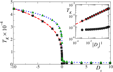
Figure 2: (Color online) Same as Fig. 1 for $\Delta_{b}=0.5$ and $\Delta_{s}=0.2$.

In Fig. 2 we show $T_{K}$ vs $D_{s}$ for a larger ratio $\Delta_{s}/\Delta_{b}=2/5$. The first obvious change with respect of the previous case is that now $T_{K}$ for negative and large in magnitude $D_{s}$ is about 50 times larger than for positive and large $D_{s}$, while in the previous case this factor was near 2. This is due to the fact that for negative $D_{s}$ both surface and bulk states contribute to the Kondo effect while for positive $D_{s}$ only the bulk states remain at the Fermi energy. Fitting as before the NCA results for $D_{s}<-0.125$ by a power law we obtain an exponent $\eta=0.2772$, again very near the PMS value $\eta=2/7=0.2857$. For positive $D_{s}$, $T_{K}$ increases slightly. In this case for $D_{s}=-D$, Eqs. (18) and Eq. (19) give $A=0.33$ and $T_{K}=4.16\times 10^{-3}$ while the NCA value is $4.44\times 10^{-3}$. For $D_{s}=D$ the corresponding values are $9.8\times 10^{-6}$ and $1.06\times 10^{-5}$. Again the NCA values are near or 8% larger than the PMS results.

The fitting of the SBMFA results for $|D_{s}|>0.125$ gives an exponent 0.142 for $D_{s}<0$ again near to $\nu=1/7=0.143$ and -0.199 for $D_{s}>0$ very near to $-\mu=-1/5$. For the comparison in Fig. 2, the SBMFA results were multiplied by 0.35, near to $A=0.33$, suggesting as before that SBMFA gives a value near to the PMS result to second order in $J$, while the NCA seems to capture higher order corrections. An additional factor 3.16 exists between SBMFA and NCA results for the point where for the NCA $T_{K}/|D_{s}|=0.1$.

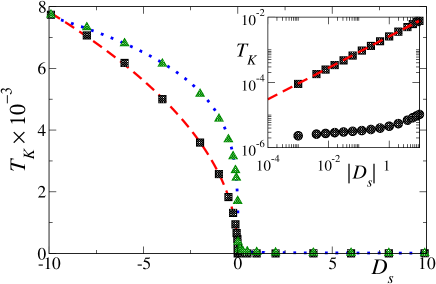
Figure 3: (Color online) Same as Fig. 1 for $\Delta_{b}=0.5$ and $\Delta_{s}=0.5$.

The case $\Delta_{s}=\Delta_{b}$ is displayed in Fig. 3. The general features are similar to those of the previous two figures, with a more dramatic difference in $T_{K}$ between negative and positive $D_{s}$ reaching three orders of magnitude. The NCA exponent of the fit for $D_{s}<-0.01$ gives $\eta=2/7=0.482$ near to the expected PMS value 1/2. As above, $T_{K}$ increases slowly for $D_{s}>0$. Here for $D_{s}=-D$, the PMS results give $A=0.40$ and $T_{K}=7.48\times 10^{-3}$ while the NCA value is $7.74\times 10^{-3}$ (3% larger). For $D_{s}=D$ the PMS value is the same as in the previous case and the NCA value is $1.05\times 10^{-5}$ (7% larger).

Fitting of the SBMFA results for $|D_{s}|>0.01$ gives exponents 0.239 and -0.496, near to the expected values 1/4 and -1/2 according to the analysis of the previous figures. The SBMFA results in the figure were were multiplied by 0.412. To see the difference between NCA and SBMFA results for small $D_{s}$, we have calculated the ratio between both of them when for the NCA $T_{K}/|D_{s}|=0.1$. Here the SBMFA gives a value 5.54 larger in the figure, or 13.4 times larger taken into account both factors.

The previous results were taken for infinite $U$ and finite $E_{d}$ for which the occupancy of the magnetic impurity fluctuates between 0 and 1, although it is near 1 in the Kondo limit. Another possible way to take this limit is to send $E_{d}\rightarrow-\infty$ together with $U\rightarrow+\infty$ keeping $E_{d}+U$ constant. This case correspond to fluctuations between a singly and double occupied impurity. The expected exponents are given by Eqs. (21). The behavior is qualitatively different from that studied so far in that $T_{K}$ is expected to be constant for $D_{s}<0$ and divergent for $D_{s}>0$ and not too small $D_{s}$. To solve one of these cases with the NCA we have performed a special electron-hole transformation that reflects the conduction bands around the Fermi energy and $E_{d}$ is changed to $-E_{d}-U$.loig .

The results in the original electron representation for $E_{d}+U=4$ and an intermediate ratio $\Delta_{s}/\Delta_{b}=2/5$ are shown in Fig. 4. In contrast to the previous cases, for negative $D_{s}$, $T_{K}$ increases with increasing $D_{s}$ reaching near 50% for $D_{s}=0$. According to Eqs. (21) one would expect a constant behavior for $D_{s}<0$. The difference might be due to terms of higher order in $J$ not included in our PMS treatment. Instead, the SBMFA predicts a decreasing $T_{K}$ with increasing $D_{s}$, which is not expected. For positive $D_{s}$ a fit of the NCA data gives an exponent $\zeta=-0.395$ in very nice agreement with $\zeta=-0.4$ given by Eqs. (21). Fitting of the SBMFA results gives exponents 0.142 for negative $D_{s}$ and -0.200 for positive $D_{s}$, again near to the values $\nu=1/7$ and $-\mu=1/5$ and in disagreement with NCA and PMS.

The PMS results for $T_{K}$ at $|D_{s}|=D$ are the same as for the case of Fig. (2) because of electron-hole symmetry in the absence of the step, namely $T_{K}=4.16\times 10^{-3}$ and $9.8\times 10^{-6}$, while the NCA values are very similar to those of that case $4.38\times 10^{-3}$ and $1.04\times 10^{-5}$. The difference might be due to an error of the order of 1% in determining $T_{K}$

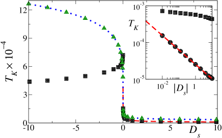
Figure 4: (Color online) Same as Fig. 1 for $E_{d}+U=4$, $\Delta_{b}=0.5$ and $\Delta_{s}=0.2$.

III.2.1 Spectral density within the NCA

The spectral density at the magnetic impurity for each spin $\rho_{d\sigma}(\omega)$ is given by Eq. (2). Due to the structure of the non-interacting part of the self-energy $\Sigma_{0\sigma}$ (see Section II) one expects that some anomaly might be present in $\rho_{d\sigma}(\omega)$ for $\omega\sim D_{s}$, particularly for large $\Delta_{s}$. In Fig. 5 we show $\rho_{d\sigma}(\omega)$ calculated with NCA for two small values of $D_{s}$ and other parameters as in Fig. 3. The main difference with usual NCA results for the spectral density is that the step in the conduction density of states is transfered through the hybridization to the impurity density of states and small steps are observed for $\omega=D_{s}$. The peak of larger spectral weight near $\omega=E_{d}$ is the charge-transfer peak. Since for $\omega\sim E_{d}$, there is no surface density of states, the total width at half maximum expected for this peak is $\sim 4\Delta_{b}=2$,capa in agreement with what we obtain. This peak is almost unchanged as $D_{s}$ crosses the Fermi energy [$\tilde{E}_{d}(E_{d})$ increases a little bit, see Eq. (8)].

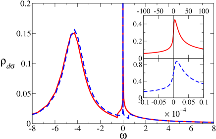
Figure 5: (Color online) Spectral density of states within NCA for $E_{d}=-4$, $\Delta_{b}=\Delta_{s}=0.5$ and two values of $D_{s}$, full line: $D_{s}=-0.5$, dashed line: $D_{s}=0.5$. The insets show details of the peaks near $\omega=0$.

Instead, the width of the Kondo peak near the Fermi energy changes dramatically. This width is of the order of the Kondo temperature $T_{K}$ and the absence of surface states for $D_{s}>0$ renders $T_{K}$ nearly three order of magnitude smaller. Mathematically this is caused by the absence of $\Delta_{s}$ in the exponent of Eq. (18). In spite of this, the shape of the Kondo peak does not change too much. Another difference apparent in the figure, is a factor near 2 between the intensity of the peak for $D_{s}>0$ compared to that for $D_{s}<0$. We remind the reader that due to the Friedel sun rule, the spectral density at the Fermi energy can be written in the form lan ; loig

$$\rho_{d\sigma}(\epsilon_{F})=\frac{\sin^{2}\varphi_{\sigma}}{\pi\Delta_{\sigma}(\epsilon_{F})},$$ (22)

where

$$\varphi_{\sigma}=\pi\langle d_{\sigma}^{\dagger}d_{\sigma}\rangle+\mathrm{Im}\int_{-\infty}^{\epsilon_{F}}d\omega G_{d\sigma}(\omega+i\epsilon)\frac{\partial\Sigma_{0\sigma}(\omega+i\epsilon)}{\partial\omega}.$$ (23)

In the usual case of a flat wide symmetric conduction band, $\partial\Sigma_{0\sigma}/\partial\omega=0$ and the integral in Eq. (23) can be neglected. This is not our case. However we expect that the influence of this term is rather small except when $\epsilon_{F}\sim D_{s}$. Taking into account that the NCA has some deviations of the order of 10% in Friedel sum rule,su42 we do not calculate the integral here. Since for both $D_{s}$ we obtain an occupancy $0.47<\langle d_{\sigma}^{\dagger}d_{\sigma}\rangle<0.5$, one expects $\varphi\sim\pi/2$ and $\rho_{d\sigma}(\epsilon_{F})$ slightly below $1/[\pi(\Delta_{b}+\Delta_{s})]\approx 0.318$ for $D_{s}<0$ and $1/(\pi\Delta_{b})\approx 0.637$ for $D_{s}>0$. The corresponding NCA values are 0.315 and 0.614 respectively. In any case NCA tends to overestimate $\rho_{d\sigma}(\epsilon_{F})$.su42

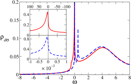
Figure 6: (Color online) Same as Fig. 5 for $E_{d}+U=4$.

In 6 we show the spectral density for the case in which the on site energies of the impurity $E_{d}$ and $E_{d}+U$ are reflected through the Fermi energy, keeping $U\rightarrow\infty$. This was calculated with NCA using an electron-hole transformation as explained in the previous section. The charge transfer peak is now located for energies above $\epsilon_{F}$ and has a width near $4(\Delta_{s}+\Delta_{b})$, wider than in the previous case, because the surface states also contribute to its width. The Kondo temperatures are larger than in the previous case, because now the shift given by the second member of Eq. (8) pushes the effective $d$ level towards the Fermi energy and then also $J$ increases [see Eq. (11)]. The structures for $\omega\sim D_{s}$ are more pronounced in this case, in particular for $D_{s}=0.5$, where one can see a pronounced peak mounted on the left side of the charge-transfer peak and probably taken some spectral weight from it. We have verified that in contrast to the Kondo peak, which as it is well known rapidly loses intensity with increasing temperature, the peak at $\omega=D_{s}$ for $D_{s}=0.5$ is practically independent of temperature for $T<T_{K}$.

Concerning the magnitude of the spectral density at the Fermi energy, we obtain with the NCA $\rho_{d\sigma}(\epsilon_{F})=0.315$ for $D_{s}<0$ and 0.597 for $D_{s}>0$, near to the maximum possible values according to the Friedel sum rule. They are likely overestimated by a few %.

III.3 Numerical renormalization group

Here we present our NRG results for the same case and parameters shown in Fig. 3. We have determined $T_{K}$ in the same way as with the NCA, namely the temperature at which the conductance through the systems falls to half the ideal value. To calculate the conductance we have calculated the Green function in each iteration which correspond to a temperature scale $\sim\lambda^{-0.5(N-1/2)}$ where $\lambda$ is the renormalization parameter and $N$ is the number of iteration, and we have used the z-trick Yoshida to reduce the errors due to discretization.

The result is shown in Fig. 7 for several values of $\Lambda$. We see that for the largest value $\Lambda=2.5$ one observes some oscillations, suggesting that the algorithm has some difficulties in representing a step at finite energies due to the logarithmic discretization. As $\Lambda$ decreases, the curve for negative $D_{s}$ approaches the dependence with $D_{s}$ expected from PMS and NCA. Unfortunately, decreasing $\Lambda$ further would require a precision that is beyond our capabilities. Concerning the magnitude of the Kondo temperature, the NRG value for $D_{s}=-D$ is $T_{K}^{0}=0.0048$, 38 % smaller than the corresponding NCA value 0.0077. For $D_{s}>0$ the behavior of $T_{K}$ is also similar to the NCA result.

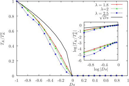
Figure 7: (Color online) Kondo temperature as a function of the bottom of the conduction band calculated with NRG for several values of $\Lambda$. The inset shows the results in log-log scale. Parameters as in Fig. 3. $T_{K}^{0}$ is the Kondo temperature for $D_{s}=-D$.

IV Summary and discussion

We have calculated the dependence of the characteristic energy scale of the Kondo effect $T_{K}$ for the impurity Anderson model in the presence of a step in the conduction density of states. This is the physical situation that takes place at the (111) surface of Cu, Ag and Au, where a two-dimensional band of surface Shockley states start at an energy $D_{s}$ slightly below the Fermi level $\epsilon_{F}$. Depending on the element, $\epsilon_{F}-D_{s}$ ranges from 67 to 475 meV. This difference can be changed by alloying the different noble metals at the surface,cerce ; abd or by applying strain, changing the sign of it,neu ; andy1 as explained in Section I.

We obtain that in the general case, as $D_{s}$ is varied, $T_{K}$ can be well described by a power law $T_{K}\simeq|D_{s}-\epsilon_{F}|^{\eta}$ for $D_{s}-\epsilon_{F}<0$ and a different power law $T_{K}\simeq(D_{s}-\epsilon_{F})^{\zeta}$ for $D_{s}-\epsilon_{F}>0$. This dependence is no more valid for very small $|D_{s}|\sim T_{K}$. The Kondo temperature is much larger for negative $D_{s}-\epsilon_{F}$ because of the presence of surface states at the Fermi energy. The exponent is in general non-trivial, except for $U\rightarrow\infty$ and $D_{s}-\epsilon_{F}>0$ ($<0$) if $E_{d}$ ($E_{d}+U$) is finite, in which case $\zeta=0$ ($\eta=0$) and $T_{K}$ slightly increases with $D_{s}$. The exponents are given by Eq. (18) and depend on the ratio between surface and bulk hybridizations with the impurity $\Delta_{s}/\Delta_{b}$ and the ratio between on-site and Coulomb energy $E_{d}/U$. Thus, changing $D_{s}-\epsilon_{F}$ by alloying or by other method, might provide a way to extract these ratios which are difficult to estimate by alternative methods.

For $|D_{s}-\epsilon_{F}|<\Delta_{s}+\Delta_{b}$ and $\Delta_{s}\gtrsim\Delta_{b}$, the spectral density of states of the magnetic impurity also shows steps or peaks at $\omega\sim D_{s}$.

We expect that our work stimulates further experimental work on the subject.

We now discuss several effects that might be present in real systems absent in our model. We have assumed a constant hybridization between the magnetic impurity added at the surface and both bulk and surface states. Actually, the important fact is that the hybridization is rather featureless in an energy range larger than $2|D_{s}|$ around the Fermi energy. In general, one expects that this should be true for sufficiently small $|D_{s}|$, if symmetry allows it. Some calculations suggest rather constant hybridization in a range of 1 eV around the Fermi energy.merino

We have also assumed a non-degenerate magnetic orbital hybridizing with bulk and surface states of the same symmetry (like a $d_{3z^{2}-r^{2}}$ localized state hybridizing with bulk and suface $s$ and $p_{z}$ states), leading to the simplest Anderson model to describe the system. In some cases degenerate orbitals are expected. For example, for iron(II) phtalocyanine (FePc) molecules on Au(111), the important orbitals are the degenerate Fe $3d$ Fe orbitals with symmetry $xz$ and $yz$ and the effective low-energy impurity model has SU(4) symmetry.mina ; mole ; joa2 Our results can be easily extended for this model and similar power-law dependences would result. However, in this case we expect that the hybridization vanishes at the bottom of the surface band for symmetry reasons. In the hypothetical case of two electrons occupying both orbitals, one has the two-channel spin-1 Kondo model, which is also a Fermi liquid dinap and we expect a similar physics.

One might wonder if Rashba spin-orbit coupling, which splits the Fermi wave vector of the surface states of Au(111) in two values (0.160 Å^-1 and 0.186 Å^-1 soc ) affects our conclusions. However, NRG calculations show that the effect on the Kondo temperature is very small.tksoc1 ; tksoc2 Therefore, except perhaps for very small $D_{s}-\epsilon_{F}$, we do not expect a significant effect.

Finally, to estimate the effect of a non sharp edge in the surface spectral density of states, we have calculated using PMS the Kondo temperature for a linear increase of $\rho_{s}$ between $D_{s}-\delta$ and $D_{s}$ with $\delta>0$ for $D_{s}<0$. To linear order in $\delta/|D_{s}|$ the result is

$$T_{K}(\delta)=T_{K}(0)\left[1+\frac{\Delta_{s}}{4(\Delta_{s}+\Delta_{b})}\frac{\delta}{|D_{s}|}\right]$$

Therefore, the correction is small except when $D_{s}$ is very near the Fermi level.

Concerning the different techniques used, we obtain a very good agreement between poor man’s scaling (PMS) on the effective Kondo model and the non-crossing approximation (NCA). Taking into account the success of both approaches in similar problems, this is a further indication that these approximations give accurate results for the Kondo temperature, apart from a factor of the order of one in the smallest non-trivial order order in PMS.

The numerical-renormalization group which is usually a very accurate technique for low-energy features has trouble in capturing the step in the conduction band, due to the logarithmic discretization of the latter.

The slave bosons in the mean-field approximation (SBMFA) gives wrong exponents for the dependence of $T_{K}$ on $D_{s}-\epsilon_{F}$. It seems to miss the renormalization of the effective exchange constant. In spite of this for not too small $|D_{s}-\epsilon_{F}|$ it gives the correct order of magnitude of $T_{K}$. Usually $|D_{s}-\epsilon_{F}|\gg T_{K}$. In one of the worst cases, Co on Ag(111), the ratio $T_{K}/(\epsilon_{F}-D_{s})$ is slightly below 0.1.serra For this ratio and some cases we have studied, the SBMFA overestimates $T_{K}$ by a factor near 4 in comparison with NCA [in addition to the prefactor $A$ in Eq. (18)], while it works better for small $\Delta_{s}$ or $E_{d}+U$ near the Fermi energy.

These results are useful for researchers studying similar problems.

References

- (1) A. C. Hewson, The Kondo Problem to Heavy Fermions (Cambridge University Press, Cambridge, England, 1997), ISBN 9780521599474.
- (2) D. Goldhaber-Gordon, H. Shtrikman, D. Mahalu, D. Abusch-Magder, U. Meirav, and M. A. Kastner, Nature 391, 156 (1998).
- (3) S. M. Cronenwett, T. H. Oosterkamp, and L. P. Kouwenhoven, Science 281, 540 (1998).
- (4) W.G. van der Wiel, S. de Franceschi, T. Fujisawa, J.M. Elzerman, S. Tarucha, and L.P. Kowenhoven, Science 289, 2105 (2000).
- (5) M. Grobis, I. G. Rau, R. M. Potok, H. Shtrikman, and D. Goldhaber-Gordon, Phys. Rev. Lett. 100, 246601 (2008).
- (6) S. Amasha, A. J. Keller, I. G. Rau, A. Carmi, J. A. Katine, H. Shtrikman, Y. Oreg, and D. Goldhaber-Gordon, Phys. Rev. Lett. 110, 046604 (2013).
- (7) W. Liang, M. P. Shores, M. Bockrath, J. R. Long, and H. Park, Nature 417, 725 (2002).
- (8) S. Kubatkin, A. Danilov, M. Hjort, J. Cornil, J. L, Brédas, N. Stuhr-Hansen, P. Hedegård, and Th. Bjö rnholm, Nature 425, 699 (2003).
- (9) J. J. Parks, A. R. Champagne, G. R. Hutchison, S. Flores-Torres, H. D. Abruña, and D. C. Ralph, Phys. Rev. Lett. 99, 026601 (2007).
- (10) N. Roch, S. Florens, V. Bouchiat, W. Wernsdorfer, and F. Balestro, Nature 453, 633 (2008).
- (11) J. J. Parks, A. R. Champagne, T. A. Costi, W. W. Shum, A. N. Pasupathy, E. Neuscamman, S. Flores-Torres, P. S. Cornaglia, A. A. Aligia, C. A. Balseiro, G. K.-L. Chan, H. D. Abruña, and D. C. Ralph, Science 328, 1370 (2010).
- (12) S. Florens, A, Freyn, N. Roch, W. Wernsdorfer, F. Balestro, P. Roura-Bas and A. A. Aligia, J. Phys. Condens. Matter 23, 243202 (2011).
- (13) R. Vincent, S. Klyatskaya, M. Ruben, W. Wernsdorfer, and F. Balestro, Nature (London) 488, 357 (2012).
- (14) J. Li, W.-D. Schneider, R. Berndt, and B. Delley, Phys. Rev. Lett. 80, 2893 (1998)
- (15) V. Madhavan, W. Chen, T. Jamneala, M. F. Crommie, and N. S. Wingreen, Science 280, 567 (1998).
- (16) H. C. Manoharan, C. P. Lutz, and D. M. Eigler, Nature (London) 403, 512 (2000).
- (17) N. Knorr, M. A. Schneider, L. Diekhöner, P. Wahl, and K. Kern, Phys. Rev. Lett. 88, 096804 (2002).
- (18) L. Limot, E. Pehlke, J. Kröger, and R. Berndt, Phys. Rev. Lett. 94, 036805 (2005).
- (19) J. Henzl and K. Morgenstern, Phys. Rev. Lett. 98, 266601 (2007).
- (20) D. Serrate, M. Moro-Lagares, M. Piantek, J. I. Pascual, and M. R. Ibarra, J. Phys. Chem. C 118, 5827 (2014).
- (21) D. M. Eigler and E. K. Schweizer, Nature (London) 344, 524 (1990).
- (22) M. F. Crommie, C. P. Lutz, and D. M. Eigler, Science 262, 218 (1993).
- (23) E. J. Heller, M. F. Crommie, C. P. Lutz, and D. M. Eigler, Nature (London) 369, 464 (1994).
- (24) G. A. Fiete and E. J. Heller, Rev. Mod. Phys. 75, 933 (2003); references therein.
- (25) A. A. Aligia and A. M. Lobos, J. Phys. Cond. Matt. 17, S1095 (2005); references therein.
- (26) M. Plihal and J. W. Gadzuk, Phys. Rev. B 63, 085404 (2001).
- (27) P. Roushan, J. Seo, C. V. Parker, Y. Hor, D. Hsieh, D. Qian, A. Richardella, M. Z. Hasan, R. Cava, and A. Yazdani, Nature (London) 460, 1106 (2009).
- (28) Y. Takahashi, T. Miyamachi, K. Ienaga, N. Kawamura, A. Ernst, and F. Komori, Phys. Rev. Lett. 116, 056802 (2016).
- (29) A. Zhao, Q. Li, L. Chen, H. Xiang, W. Wang, S. Pan, B. Wang, X, Xiao, J.Yang, J. G. Hou, and Q. Zhu, Science 309, 1542 (2005)
- (30) T. Komeda, H. Isshiki, J. Liu, Y-F. Zhang, N. Lorente, K. Katoh, B. K. Breedlove, and M. Yamashita, Nat. Commun. 2, 217 (2011).
- (31) E. Minamitani, N. Tsukahara, D. Matsunaka, Y. Kim, N. Takagi, and M. Kawai, Phys. Rev. Lett. 109, 086602 (2012).
- (32) V. Iancu, K. Shouteden, Z. Li, and C. Van Haesendonck, Chem. Commun. 52, 11359 (2016).
- (33) S. L. Hulbert, P. D. Johnson, N. G. Stoffel, W. A. Royer, and N. V. Smith, Phys. Rev. B 31, 6815 (1985).
- (34) H. Cercellier, C. Didiot, Y. Fagot-Revurat, B. Kierren, L. Moreau, D. Malterre, and F. Reinert, Phys. Rev. B 73, 195413 (2006).
- (35) Z. M. Abd El-Fattah, M. Matena, M. Corso, M. Ormaza, J. E. Ortega, and F. Schiller, Phys. Rev. B 86, 245418 (2012); references therin.
- (36) A. Euceda, D.M. Bylander, and L. Kleinman, Phys. Rev. B 28, 528 (1983).
- (37) B. Yan, B. Stadtmüller, N. Haag, S. Jakobs, J. Seidel, D. Jungkenn, S. Mathias, M. Cinchetti, M. Aeschlimann, and C. Felser, Nature Commun. 6, 10167 (2015).
- (38) J. Fernández, M. Moro-Lagares, D. Serrate, and A. A. Aligia, Phys. Rev. B 94, 075408 (2016)
- (39) A. A. Aligia, Phys. Rev. B 64, 121102(R) (2001).
- (40) D. Porras, J. Fernández-Rossier, and C. Tejedor, Phys. Rev. B 63, 155406 (2001).
- (41) M. Weissmann and H. Bonadeo, Physica E (Amsterdam) 10, 44 (2001).
- (42) K. Hallberg, A. A. Correa, and C. A. Balseiro, Phys. Rev. Lett. 88, 066802 (2002).
- (43) A. A. Aligia, Phys. Status Solidi (b) 230, 415 (2002).
- (44) G. Chiappe and A. A. Aligia, Phys. Rev. B 66, 075421 (2002).
- (45) Q. Li, S. Yamazaki, T. Eguchi, H. Kim, S.-J. Kahng, J. F. Jia, Q. K. Xue, and Y. Hasegawa, Phys. Rev. B, 80, 115431 (2009).
- (46) J. Merino and O. Gunnarsson, Phys. Rev. Lett. 93, 156601 (2004).
- (47) M. A. Barral, A. M. Llois, and A. A. Aligia, Phys. Rev. B 70, 035416 (2004).
- (48) Baruselli, P. P. and Requist, R. and Smogunov, A. and Fabrizio, M. and Tosatti, E., Phys. Rev. B, 92, 045119 (2015).
- (49) M. Moro-Lagares, Ph. D. thesis, Universidad de Zaragoza, Spain (2015).
- (50) G. Neuhold and K. Horn, Phys. Rev. Lett. 78, 1327 (1997).
- (51) C. W. Hicks, M. E. Barber, S. D. Edkins, D. O. Brodsky and A. P. Mackenzie, Rev. Sci. Inst. 65, 65003 (2014).
- (52) C. W. Hicks, D. O. Brodsky, E. A. Yelland, A. S. Gibbs, J. A. N. Bruin, M. E. Barber, S. D. Edkins, K. Nishimura, S. Yonezawa, Y. Maeno and A. P. Mackenzie, Science 344, 283 (2014).
- (53) P. W. Anderson, J. Phys. C 3, 2439 (1970).
- (54) N.E. Bickers, Rev. of Mod. Phys. 59, 845 (1987).
- (55) P. Coleman, Phys. Rev. B 29, 3035 (1984); 35, 5072 (1987)
- (56) D. M. Newns and N. Read, Adv. Phys. 36, 799 (1987).
- (57) Bulla, Ralf and Costi, Theo A. and Pruschke, Thomas, Rev. Mod. Phys., 80, 395 (2008).
- (58) K. G. Wilson, Reviews of Modern Physics 47, 773 (1975).
- (59) D M Cragg, P Lloyd and P Nozieres, Journal of Physics C: Solid State Physics, 13, 803 (1980).
- (60) H. R. Krishna-murthy, J. W. Wilkins, and K. G. Wilson, Physical Review B 21, 1003 (1980).
- (61) V. L. Campo Jr and L. N. Oliveira, Phys. Rev. B 72, 104432 (2005).
- (62) J. Kroha and P. Wölfle, Acta Phys. Pol. B 29, 3781 (1998).
- (63) R. Žitko, Phys. Rev. B 84, 085142 (2011).
- (64) L. Vaugier, A.A. Aligia and A.M. Lobos, Phys. Rev. B 76, 165112 (2007).
- (65) A. A. Aligia, P. Roura-Bas, and S. Florens, Phys. Rev. B 92, 035404 (2015).
- (66) Th. Pruschke and N. Grewe, Z. Phys. B 74, 439 (1989).
- (67) D. E. Logan, M. P. Eastwood, and M. A. Tusch, J. Phys. Condens. Matter 10, 2673 (1998).
- (68) J. Könemann, B. Kubala, J. König, and R. J. Haug, Phys. Rev. B 73, 033313 (2006).
- (69) N. S. Wingreen and Y. Meir, Phys. Rev. B 49, 11040 (1994).
- (70) F. Reinert, D. Ehm, S. Schmidt, G. Nicolay, S. Hüfner, J. Kroha, O. Trovarelli, and C. Geibel, Phys. Rev. Lett. 87, 106401 (2001).
- (71) D. Ehm, S. Hüfner, F. Reinert, J. Kroha, P. Wölfle, O. Stockert, C. Geibel, and H. v. Löhneysen, Phys. Rev. B 76, 045117 (2007).
- (72) L. Tosi, P. Roura-Bas, and A. A. Aligia, J. Phys.: Condens. Matter 27 335601 (2015).
- (73) S. Di Napoli, P. Roura-Bas, A. Weichselbaum and A. A. Aligia, Phys. Rev. B 90, 125149 (2014).
- (74) P. Roura-Bas and A. A. Aligia, Phys. Rev. B 80, 035308 (2009); J. Phys. Condens. Matt. 22, 025602 (2010).
- (75) A. C. Hewson, J. Bauer, and A. Oguri, J. Phys.: Condens. Matter 17, 5413 (2005), and references therein.
- (76) A. A. Aligia, Phys. Rev. B 89, 125405 (2014), and references therein.
- (77) M. Romero and A. A. Aligia, Phys. Rev. B 83, 155423 (2011)
- (78) X-Y. Feng, J. Dai, C-H. Chung, and Q. Si, Phys. Rev. Lett. 111, 016402 (2013).
- (79) A. M. Lobos, M. A. Romero, and A. A. Aligia, Phys. Rev. B 89, 121406(R) (2014).
- (80) J. Fernández, A. A. Aligia, and A. M. Lobos, Europhys. Lett. 109, 37011 (2015).
- (81) D. C. Langreth, Phys. Rev. 150, 516 (1966).
- (82) A. Lobos and A. A. Aligia, Phys. Rev. B 68, 035411 (2003).
- (83) J. R. Schrieffer and P. A. Wolff, Phys. Rev. 149, 491 (1966).
- (84) J. Sólyom and A. Zawadosky, J. Phys. F 4, 80 (1974).
- (85) Th. Pruschke and N. Grewe, Z. Phys. B - Condensed Matter 74, 439 (1989).
- (86) K. Haule, S. Kirchner, J. Kroha, and P. Wölfle, Phys. Rev. B 64, 155111 (2001).
- (87) L. Tosi, P. Roura-Bas, A. M. Llois, and L. O. Manuel, Phys. Rev. B 83, 073301 (2011).
- (88) L. Tosi, P. Roura-Bas, A. M. Llois and A. A. Aligia, Physica B 407, 3263 (2012).
- (89) L. Tosi, P. Roura-Bas, and A. A. Aligia, Physica B 407, 3259 (2012).
- (90) M. Yoshida, M. A. Whitaker, and L. N. Oliveira, Phys. Rev. B 41, 9403 (1990).
- (91) S. Di Napoli, M. A. Barral, P. Roura-Bas, L. O. Manuel, A. M. Llois, and A. A. Aligia, Phys. Rev. B 92, 085120 (2015).
- (92) J. Henk, M. Hoesch, J. Osterwalder, A. Ernst and P. Bruno, J. Phys.: Condens. Matter 16 , 7581 (2004).
- (93) R. Žitko and J. Bonča, Phys. Rev. B 84, 193411 (2011).
- (94) A. Wong, S. E. Ulloa, N. Sandler, and K. Ingersent, Phys. Rev. B 93, 075148 (2016).