3D Simulation of Spindle Gravitational Collapse
of a Collisionless Particle System

Abstract

We simulate the spindle gravitational collapse of a collisionless particle system in a 3D numerical relativity code and compare the qualitative results with the old work done by Shapiro and Teukolsky Shapiro:1991zza . The simulation starts from the prolate-shaped distribution of particles and a spindle collapse is observed. The peak value and its spatial position of curvature invariants are monitored during the time evolution. We find that the peak value of the Kretschmann invariant takes a maximum at some moment, when there is no apparent horizon, and its value is greater for a finer resolution, which is consistent with what is reported in Ref. Shapiro:1991zza . We also find a similar tendency for the Weyl curvature invariant. Therefore, our results lend support to the formation of a naked singularity as a result of the axially symmetric spindle collapse of a collisionless particle system in the limit of infinite resolution. However, unlike in Ref. Shapiro:1991zza , our code does not break down then but go well beyond. We find that the peak values of the curvature invariants start to gradually decrease with time for a certain period of time. Another notable difference from Ref. Shapiro:1991zza is that, in our case, the peak position of the Kretschmann curvature invariant is always inside the matter distribution.

I Introduction

Gravitational collapse is one of the most typical and attractive phenomena in general relativity. The singularity theorem (see, e.g., Ref. Hawking:1973uf ) states that the formation of spacetime singularities is inevitable as a result of gravitational collapse with physically reasonable matter fields. If the cosmic censorship conjecture, proposed by Penrose 1969NCimR…1..252P ; 2002GReGr..34.1141P ; Penrose1979 , is valid, those singularities generated from general and physically reasonable initial data should be clothed by a black hole horizon. Visible spacetime singularities are so-called naked singularities and a bunch of examples for a naked singularity are reported in various spacetimes. Generality of naked singularity formation is an important open issue in general relativity.

The cosmic censorship conjecture and naked singularity formation is of interest not only in a mathematical aspect of general relativity, but also in finding the cut-off energy scale of general relativity. In other words, a spacetime domain near a naked singularity with infinite curvature, which we call a border of spacetime Harada:2004mv , may be a window into new physics beyond general relativity. Even if the curvature scale does not exceed the cut-off scale, it would provide the locally high energy region in which unknown high energy particle physics phenomena may take place. The higher curvature regions associated with gravitational collapse would provide a key to understand unsolved problems in cosmology, astrophysics and high energy particle physics.

In this paper, we focus on non-spherical gravitational collapse. As is stated by the hoop conjecture Thorne1972 , a gravitational source with a sufficiently large circumference compared to its gravitational radius cannot form a black hole with a horizon. Therefore, we expect that the gravitational collapse which causes a highly elongated or flattened object at the end may not be surrounded by a black hole horizon and produces a spacetime border. One of the most famous examples has been presented by Shapiro and Teukolsky (ST) Shapiro:1991zza , where the violation of the cosmic censorship conjecture due to spindle gravitational collapse of collisionless ring sources is discussed assuming axisymmetry. Our purpose in this letter is the reanalysis of this system by using recently developed numerical relativity techniques without exact axisymmetry.

Shapiro and Teukolsky Shapiro:1991zza firstly dealt with relativistic collisionless matter in axisymmetric spacetimes (see Ref. Yamada:2011br for a higher-dimensional version). Full 3-dimensional simulations of relativistic collisionless particle systems have been performed by Shibata in Refs. Shibata:1999 ; Shibata:1999wi . We basically follow the methods adopted in Refs. Shibata:1999 ; Shibata:1999wi . The specifications of our numerical procedure are described in Sec. II.

In this paper, we use the geometrized units in which both the speed of light and Newton’s gravitational constant are one.

II Summary of Methods

II.1 Geometrical Variables

In this paper, we solve time evolution based on the so called BSSN formalism Shibata:1995we ; Baumgarte:1998te with a method of 2nd order finite differences. The maximal slicing and the hyperbolic gamma driver Alcubierre:2002kk are adopted for the gauge conditions. For stable calculations, we implement the Kreiss-Oliger Kreiss-Oliger dissipation. Although we do not write all equations down, just to fix the notation, we start with introducing geometrical and matter variables for the numerical integration. Readers may refer to several textbooks on numerical relativity(e.g., Refs. 2010nure.book…..B ; Gourgoulhon:2007ue ; shibata2016numerical ) for details.

We consider the following form of line elements:

$$\mathrm{d}s^{2}=-\alpha^{2}\mathrm{d}t^{2}+\gamma_{ij}\left(\mathrm{d}x^{i}+\beta^{i}\mathrm{d}t\right)\left(\mathrm{d}x^{j}+\beta^{j}\mathrm{d}t\right),$$ (1)

where $i,j=1,2,3$, and $\gamma_{ij}$, $\alpha$ and $\beta^{i}$ are the spatial metric, lapse function and shift vector, respectively. The Roman indices are lowered and raised by the spatial metric $\gamma_{ij}$. For numerical integration, we use the Cartesian coordinate system and decompose the spatial metric as

$$\gamma_{ij}={\rm e}^{4\psi}\tilde{\gamma}_{ij}~{}~{}{\rm with}~{}~{}\det\tilde{\gamma}=1.$$ (2)

The unit normal vector field $n^{\mu}$ to the spatial hyper-surface is given by $n_{\mu}=-\alpha\left(\mathrm{d}t\right)_{\mu}$, where the Greek index $\mu$ runs from 0 to 3. Then, the projection tensor $\gamma_{\mu}^{~{}\nu}$ satisfying $\gamma_{\mu}^{~{}\nu}n_{\nu}=0$ is given by

$$\gamma_{\mu}^{~{}\nu}=n_{\mu}n^{\nu}+g_{\mu}^{~{}\nu}.$$ (3)

The extrinsic curvature $K_{ij}$ is defined by

$$K_{ij}=-\gamma_{i}^{~{}\mu}\gamma_{j}^{~{}\nu}\nabla_{\mu}n_{\nu}.$$ (4)

We adopt the following decomposition of the extrinsic curvature:

$$K_{ij}={\rm e}^{4\psi}\tilde{A}_{ij}+\frac{1}{3}K\gamma_{ij},$$ (5)

where $K$ and ${\rm e}^{4\psi}\tilde{A}_{ij}$ are the trace and traceless parts of the extrinsic curvature $K_{ij}$. Then, the Einstein equations can be written in terms of $\alpha$, $\beta^{i}$, $\gamma_{ij}$($\tilde{\gamma}_{ij}$ and $\psi$) and $K_{ij}$($\tilde{A}_{ij}$ and $K$). For example, the Hamiltonian and momentum constraints are written as

$$16\pi E-R-K^{2}+K_{ij}K^{ij} = 0,$$ (6)

$$\mathcal{M}^{i}:=8\pi J^{i}-D_{j}K^{ji}+D^{i}K = 0,$$ (7)

where $R$ and $D_{i}$ are the scalar curvature and the covariant derivative with respect to $\gamma_{ij}$, and $E$ and $J^{i}$ are defined by using the stress energy tensor $T^{\mu\nu}$ as follows:

$$E = n_{\mu}n_{\nu}T^{\mu\nu},$$ (8)

$$J^{i} = -\gamma^{i}_{~{}\mu}n_{\nu}T^{\mu\nu}.$$ (9)

For a later convenience, we also introduce the following variable:

$$S^{ij}=\gamma^{i}_{~{}\mu}\gamma^{j}_{~{}\nu}T^{\mu\nu}.$$ (10)

II.2 Stress energy tensor for a collisionless particle system

Let us consider the collisionless particle system composed of $N$ particles each of which travels a timelike geodesic. The four velocity $u^{\mu}_{p}$ of the particle labelled by a positive integer $p$ can be decomposed as follows Vincent:2012kn :

$$u_{p}^{\mu}=\Gamma_{p}\left(n^{\mu}+V_{p}^{\mu}\right),$$ (11)

where the spatial velocity components $V_{p}^{\mu}$ satisfy $V_{p}^{\mu}n_{\mu}=0$, and $\Gamma_{p}$ is the Lorentz factor. Then, the 3+1 decomposition of the geodesic equations is expressed as follows Vincent:2012kn :

$$\frac{\mathrm{d}\Gamma_{p}}{\mathrm{d}t} = \Gamma_{p}V_{p}^{i}\left(\alpha K_{ij}V_{p}^{j}-\partial_{i}\alpha\right),$$ (12)

$$\frac{\mathrm{d}V_{p}^{j}}{\mathrm{d}t} = \alpha V_{p}^{j}\left[V_{p}^{i}\left(\partial_{j}\ln\alpha-K_{jk}V_{p}^{k}\right)+2K^{i}_{~{}j}-V_{p}^{k}\Gamma^{i}_{jk}\right]-\gamma^{ij}\partial_{j}\alpha-V_{p}^{j}\partial_{j}\beta^{i},$$ (13)

$$\frac{\mathrm{d}\tau_{p}}{\mathrm{d}t} = \frac{\alpha}{\Gamma_{p}},$$ (14)

where $\tau_{p}$ is the proper time and $\mathrm{d}/\mathrm{d}t=\frac{\alpha}{\Gamma_{p}}u_{p}^{\mu}\partial_{\mu}$.

The energy momentum tensor for a particle system is given by (see, e.g., Misner:1974qy )

$$T^{\mu\nu}=-\sum_{p}m_{p}\frac{\delta^{3}\left(\bm{x}-\bm{x}_{p}\right)}{u^{\lambda}_{p}n_{\lambda}\sqrt{\gamma}}u^{\mu}_{p}u^{\nu}_{p},$$ (15)

where $m_{p}$ is the proper mass of the particle and $\bm{x}$ and $\bm{x}_{p}$ denote the spatial coordinates and those values at the particle position, respectively. Then, from Eqs. (8–10), we obtain

$$E = \sum_{p}m_{p}\Gamma_{p}\frac{\delta^{3}\left(\bm{x}-\bm{x}_{p}\right)}{\sqrt{\gamma}},$$ (16)

$$J^{i} = \sum_{p}m_{p}\Gamma_{p}V^{i}_{p}\frac{\delta^{3}\left(\bm{x}-\bm{x}_{p}\right)}{\sqrt{\gamma}},$$ (17)

$$S^{ij} = \sum_{p}m_{p}\Gamma_{p}V^{i}_{p}V^{j}_{p}\frac{\delta^{3}\left(\bm{x}-\bm{x}_{p}\right)}{\sqrt{\gamma}}.$$ (18)

In this paper, we assume that the proper mass of every particle is identical to $m$.

Since the delta function cannot be numerically treated, we introduce the following smoothing:

$$\delta^{3}\left(\bm{x}-\bm{x}_{p}\right)\rightarrow f_{\rm sp}\left(\left|\bm{x}-\bm{x}_{p}\right|,r_{\rm s}\right)$$ (19)

with

$$f_{\rm sp}(r,r_{\rm s})=\frac{1}{\pi r_{\rm s}^{3}}\left\{\begin{array}[]{lll}1-\frac{3}{2}\left(\frac{r}{r_{\rm s}}\right)^{2}+\frac{3}{4}\left(\frac{r}{r_{\rm s}}\right)^{3}&{\rm for}&0\leq\frac{r}{r_{\rm s}}\leq 1\\ \frac{1}{4}\left(2-\frac{r}{r_{\rm s}}\right)^{3}&{\rm for}&1\leq\frac{r}{r_{\rm s}}\leq 2\\ 0&{\rm for}&2<\frac{r}{r_{\rm s}}\end{array}\right.,$$ (20)

where $r_{\rm s}$ characterizes the size of a particle.

II.3 Cleaning of the Hamiltonian constraint violation

In order to reduce the violation of the Hamiltonian constraint, we update the conformal factor $\psi$ at each time step. The update is done by using the iteration steps of the Successive Over-Relaxation (SOR) method for solving the elliptic equation of the Hamiltonian constraint. The Hamiltonian constraint (6) can be rewritten in the following form:

$$\tilde{D}_{i}{\tilde{D}}^{i}\psi=-\tilde{D}_{i}\psi{\tilde{D}}^{i}\psi+\frac{1}{8}\tilde{R}+{\rm e}^{4\psi}\left(\frac{1}{12}K^{2}-\frac{1}{8}\tilde{A}_{ij}{\tilde{A}}^{ij}-2\pi E\right),$$ (21)

where $\tilde{D}_{i}$ and $\tilde{R}$ are the covariant derivative and Ricci scalar with respect to $\tilde{\gamma}_{ij}$. The iteration step is repeated only a few times depending on the degree of the violation. This prescription reduces the violation of the Hamiltonian constraint during the time evolution.

II.4 Flow of time evolution

We use the 2nd order leap frog method with time filtering for the time evolution. In our calculation, we slightly modified the evolution of ${\tilde{\Gamma}}^{i}$ defined by $-\partial_{i}{\tilde{\gamma}}^{ij}$ from that in the conventional BSSN scheme as follows:

$$\frac{\partial{\tilde{\Gamma}}^{i}}{\partial t}=\left[\frac{\partial{\tilde{\Gamma}}^{i}}{\partial t}\right]_{\rm BSSN}-2{\rm e}^{4\psi}\mathcal{M}^{i},$$ (22)

where the first term in the right-hand side represents the conventional terms in the BSSN scheme(see, e.g., Refs. 2010nure.book…..B ; Gourgoulhon:2007ue ; shibata2016numerical ). This modification does not make any qualitative difference in the results, but reduces the momentum constraint violation by a factor of a few in our simulation(see, e.g., Refs. Frittelli:1996wr ; Kidder:2001tz for similar prescriptions). It should be noted that the added term is trivial if the momentum constraints are well satisfied. The reason for the smaller momentum constraint violation is not clear and further careful investigation would be needed for other practical application of this procedure. But, we do not pursue the reason further in this paper since the modification does not make any qualitative difference in our case.

The flow of the calculation is as follows:

1. Starting from the initial data, we calculate next step geometrical variables except for $\alpha$. Variables for each particle are also evolved by using the geodesic equations, where geometrical variables at each particle position are calculated by using a 2nd order interpolation.

2. The energy momentum tensor is calculated from the particle distribution. Here, we note that the expressions (8–10) are independent of $\alpha$ which has not been fixed yet.

3. $\psi$ is updated by the cleaning of the Hamiltonian constraint violation.

4. By solving the elliptic equation of the maximal slice condition, we obtain $\alpha$.

The above procedure is repeated.

III Shapiro-Teukolsky Collapse with particles

III.1 Initial Data Construction

As in Ref. Shapiro:1991zza , we start with conformally flat and momentarily static initial data, that is,

$$\tilde{\gamma}_{ij}=\delta_{ij}~{},~{}~{}K_{ij}=0.$$ (23)

The momentum constraint equation (7) is trivially satisfied by setting $J^{i}=0$. In terms of particle variables, we assume $\Gamma_{p}=1$ and $V^{i}_{p}=0$ for every particle. The Hamiltonian constraint equation is written as

$$\triangle\Psi=-2\pi E\Psi^{5}=-2m\sum_{p}f_{\rm sp}\left(\left|\bm{x}-\bm{x}_{p}\right|,r_{\rm s}\right)/\Psi,$$ (24)

where $\Psi={\rm e}^{\psi}$ and $\triangle$ is the Laplace operator in the 3-dimensional Euclidean space. This equation can be solved by using SOR method once the particle distribution is fixed. We generate the particle distribution with reference to a continuous density distribution and the corresponding conformal factor denoted by $\bar{E}$ and $\bar{\Psi}$, respectively.

Following Refs. Shapiro:1991zza ; Nakamura:1988zq , we determine the particle distribution based on the following continuum density distribution:

$$\frac{1}{2}\bar{E}\bar{\Psi}^{5}=E_{\rm N}:=\left\{\begin{array}[]{lll}\frac{3M_{\rm N}}{4\pi a^{2}b}&{\rm for}&\frac{x^{2}+y^{2}}{a^{2}}+\frac{z^{2}}{b^{2}}\leq 1\\ 0&{\rm for}&\frac{x^{2}+y^{2}}{a^{2}}+\frac{z^{2}}{b^{2}}>1\end{array}\right.,$$ (25)

where $M_{\rm N}$ is a constant which represents the total Newtonian rest mass, $a$ is the equatorial radius and $b$ is the radius of the major axis. Then, $\bar{\Psi}$ can be expressed by the Newtonian potential $\Phi$ as follows:

$$\bar{\Psi}=1-\Phi$$ (26)

with

$$\triangle\Phi=4\pi E_{\rm N}.$$ (27)

For a prolate ($a<b$) spheroid, we obtain 1969efe..book…..C ; Nakamura:1988zq

$$\Phi = -\frac{3M_{\rm N}}{2be}\beta-\frac{3M_{\rm N}}{4b^{3}e^{3}}\left(\beta-\sinh\beta\cosh\beta\right)R^{2}-\frac{3M_{\rm N}}{2b^{3}e^{3}}\left(\tanh\beta-\beta\right)z^{2},$$ (28)

where $e=\sqrt{1-a^{2}/b^{2}}$ and $R=\sqrt{x^{2}+y^{2}}$, and $\beta$ satisfies

$$\begin{array}[]{lll}\sinh\beta=\frac{be}{a}&{\rm for}{}&\frac{x^{2}+y^{2}}{a^{2}}+\frac{z^{2}}{b^{2}}\leq 1,\\ R^{2}\sinh^{2}\beta+z^{2}\tanh^{2}\beta=b^{2}e^{2}&{\rm for}{}&\frac{x^{2}+y^{2}}{a^{2}}+\frac{z^{2}}{b^{2}}>1.\end{array}$$ (29)

Since the asymptotic behaviour in the limit $r=\sqrt{x^{2}+y^{2}+z^{2}}\rightarrow\infty$ is given by

$$\lim_{r\rightarrow\infty}\bar{\Psi}=1-\lim_{r\rightarrow\infty}\Phi=1+\frac{M_{\rm N}}{r},$$ (30)

taking the isotropic coordinate into account, the total mass $M$ can be read off as $2M_{\rm N}$.

By using this density distribution as the reference, the number of particles $\Delta N$ in a grid box with the volume $\Delta V$ is set by

$$\Delta N=\frac{\bar{E}\bar{\Psi}^{6}}{m}\Delta V=\frac{2E_{\rm N}\bar{\Psi}}{m}\Delta V,$$ (31)

where the mass $m$ is related to the total number of particles $N$ as

$$mN=M_{0}:=\int\bar{E}\bar{\Psi}^{6}\mathrm{d}^{3}x=\int 2E_{\rm N}\bar{\Psi}\mathrm{d}^{3}x=2M_{\rm N}+\frac{6}{5}\frac{M_{\rm N}^{2}}{be}\ln\frac{1+e}{1-e}.$$ (32)

We randomly distribute $N$ particles in accordance with Eq. (31), and numerically solve Eq. (24). Here, we note that, whereas the reference density distribution of the continuum is the same as that in ST, exact axisymmetry is not assumed in our case unlike in the ST case. This is because the real density distribution is composed of the particles which are randomly distributed.

III.2 Results for the same parameter setting as ST

We consider the domain for the numerical calculation given by $0<x^{i}/L<1$, where $x^{i}=(x,y,z)$. Hereafter, we normalize all dimensionful quantities in the unit of $M$. We consider the situation characterized by the following parameter set:

$$\frac{L}{M}=20~{},~{}~{}\frac{b}{M}=10~{},~{}~{}e=0.9.$$ (33)

The values of $b/M$ and $e$ are equivalent to those in ST. The initial data given by this parameter set result in a spindle collapse without an apparent horizon. In the calculation, the grid interval $\Delta$, particle size $r_{\rm s}$ and particle number $N$ are set as

$$\Delta=L/120~{},~{}~{}N=10^{6}~{},~{}~{}r_{\rm s}=L/75.$$ (34)

We have also performed a set of simulations of the physically identical model with several different resolutions. Changing the grid interval $\Delta$, we impose the following scaling for the particle size $r_{\rm s}$ and number $N$:

$$r_{\rm s}\propto\Delta~{},~{}~{}N\propto 1/\Delta^{3},$$ (35)

so that $\Delta N$, the number of particles in a grid box, is kept constant. We have checked that the dynamics of the system does not significantly depend on the size and shape of the particle profile(see Ref. Yamada:2011br for results with a Gaussian shape). All figures are for the case of $\Delta=L/120$ unless otherwise noted. We note that, in order to minimize the dispersion in dependence on the resolution, we use a common pseudo random numbers to generate particle distribution for each resolution. Therefore, a part of particles have identical initial positions for each resolution.

We emphasize that we have monitored the existence of an apparent horizon covering the origin of the coordinates during the time evolution starting from the initial data given in the previous section and concluded that there is no horizon during the time evolution. On the other hand, as will be shown in the next subsection, starting from a different initial data set, we have found an example in which an apparent horizon is finally formed after a spindle collapse. We have also monitored the violation of constraint equations (Fig. 1).

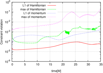
Figure 1: Constraint violations are depicted as functions of time. The violation of the Hamiltonian constraint and the momentum constraints is evaluated at each grid point using an appropriate normalization. The L1-norm and max-norm are calculated for each constraint and plotted as functions of time.

We found that suppressing the max-norm of the momentum constraint violation is relatively hard with our numerical scheme. In this subsection, we require that the max-norm of the momentum constraint violation is at most at the level of 10%. The resolution dependence of the L1-norm of the momentum constraint violation is shown in Fig. 2.

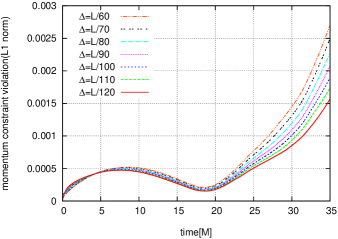
Figure 2: L1-norm of the momentum constraint violation is depicted as a function of time for each resolution.

It should be noted that, since we scale the total number and size of particles depending on the grid interval, the usual second order convergence cannot be expected(see Appendix for the second order convergence with fixed number and size of particles). Nevertheless, Fig. 2 shows that the constraint violation is smaller for a finer resolution at late times. We also note that in our simulation the convergence is not clear for local quantities without averaging due to the randomness of the particle distribution.

First, we show the snapshots of the particle distribution and density distribution, the values of the Kretschmann curvature invariant $\mathcal{K}:=R_{\mu\nu\rho\lambda}R^{\mu\nu\rho\lambda}$ and the Weyl curvature invariant $\mathcal{W}:=C_{\mu\nu\rho\lambda}C^{\mu\nu\rho\lambda}$ on the $x$-$z$ plane, where $C_{\mu\nu\rho\lambda}$ is the Weyl curvature.

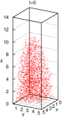
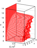
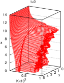
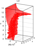
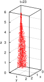
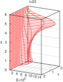
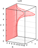
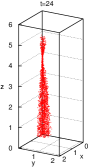
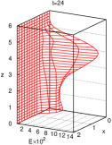
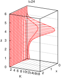
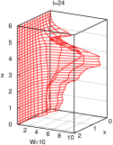
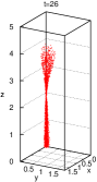
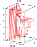
Figure 3: Snapshots of the particle distribution and density distribution, Kretschmann curvature invariant $\mathcal{K}$ and Weyl curvature invariant $\mathcal{W}$ on the $x$-$z$ plane are shown. The numerical value of every dimensionful variable is given in the unit of $M$. The snapshots at $t=23M$ are shown for comparison with figures in ST. The peak values $\mathcal{K}_{\rm p}$ and $\mathcal{W}_{\rm p}$ take the maximum values at $t\simeq 24M$ and $t\simeq 25M$, respectively.

Since our shift gauge condition is different from that used in ST, the spatial shape of the particle distribution in our coordinates cannot be directly compared with that in ST in the strict sense. Nevertheless, as is shown in Fig.  3, at $t=23M$, we can find a matter concentration near $z=5M$ similarly to the result in ST. Around this time, the system experiences the first caustic near the top of the matter distribution. We note that, unlike in ST Shapiro:1991zza , our calculation does not break down even after this time. After the first caustic, the particles which went through the caustic start to spread outward from the $z$-axis. The total length of $z$-direction continues to shrink, and the position of the caustic moves inward toward the origin.

At $t=24M$, the value of $\mathcal{K}$ has a peak at a point near the density peak. Around this time, the peak value $\mathcal{K}_{\rm p}$ takes the maximum value $\mathcal{K}_{\rm max}$ and gradually decreases with time after that. The value of $\mathcal{W}$ at its peak, denoted by $\mathcal{W}_{\rm p}$, takes the maximum value $\mathcal{W}_{\rm max}$ around $t=25M$ soon after the time when $\mathcal{K}_{\rm p}=\mathcal{K}_{\rm max}$. The values of $\mathcal{K}_{\rm p}$ and $\mathcal{W}_{\rm p}$ are depicted as functions of time in Fig. 4. As is similar to FIG. 3 in ST, the value of $\mathcal{K}_{\rm p}$ starts to increase around $t\simeq 20M$, and we find faster growth for a finer resolution.

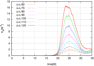
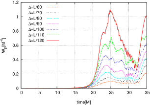
Figure 4: $\mathcal{K}_{\rm p}$ and $\mathcal{W}_{\rm p}$ are depicted as functions of time.

In spite of the dynamics qualitatively similar to that reported in ST, we can also find a significant difference from ST. In ST, it is reported that the peak position of the curvature invariant at $t=23M$ is at $\simeq 6.1M$ outside the matter distribution. While in our case, the functional form of $\mathcal{K}$ roughly traces the form of the density distribution. The main contribution for $\mathcal{K}_{\rm p}$ comes from the Ricci part of the curvature. Since the density is also divergent near the peak of $\mathcal{K}$, one may be concerned with a small trapped region in the vicinity of the peak. If the size of the trapped region is as small as a few grid intervals, our apparent horizon finder can not resolve it. Therefore, in order to investigate the existence of the small trapped region, we calculate the value of expansion $\Theta$ on the spheres centered at the peak of $\mathcal{K}$ instead of searching for the apparent horizon. The expansion $\Theta$ is defined by

$$\Theta=D_{i}s^{i}+K_{ij}s^{i}s^{j}-K,$$ (36)

where $s^{i}$ is the unit normal vector to the sphere. In Fig. 5, we depict the value of $\Theta$ averaged on each sphere as a function of the radius of the sphere.

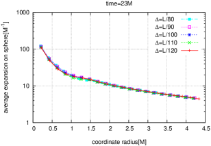
Figure 5: The averaged value of $\Theta$ is depicted as a function of the radius of the sphere for each resolution.

As is shown in Fig. 5, the average value of $\Theta$ is positive at least within our resolution. This suggests nonexistence of such an apparent horizon.

Finally, let us check how $\mathcal{K}_{\rm max}$ and $\mathcal{W}_{\rm max}$ depend on the numerical resolution. In Fig. 6, $\mathcal{K}_{\rm max}$ and $\mathcal{W}_{\rm max}$ are depicted as functions of the grid interval $\Delta$, where $\mathcal{W}_{\rm max}$ is evaluated within the time interval $0\leq t<30M$. The behaviour of $\mathcal{K}_{\rm max}$ for smaller $\Delta$ seems to have an inverse power dependence on $\Delta$. We also find similar tendency for $\mathcal{W}_{\rm max}$. These dependences suggest divergent curvature invariants in the limit of infinite resolution similarly to ST.

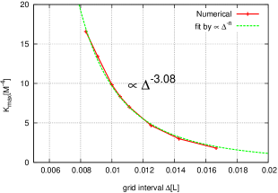
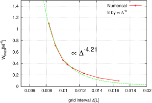
Figure 6: $\mathcal{K}_{\rm max}$ and $\mathcal{W}_{\rm max}$ are depicted as functions of the grid interval $\Delta$.

III.3 Results for a larger mass system

As is written in the section III.2, we did not find an apparent horizon for the same parameter setting as the ST case. In the sense of the hoop conjectureThorne1972 , we expect that a trapped region can be more easily formed for a larger mass system with the same size and shape of the matter distribution. In this subsection, we show an example in which an apparent horizon is formed after the occurrence of the maximum value of the Kretschmann invariant by increasing the total mass comparing the grid interval. It is also worthy to note that, since the total mass of the previous system is given by $M=6\Delta$, the corresponding horizon radius in the isotropic coordinate is given by $M/2=3\Delta$. Therefore, the resolution seems to be not enough to resolve the spherical horizon for the Schwarzschild black hole with the same mass $M$.

Let us consider the particle distribution generated by the following parameter set:

$$\frac{L}{M}=\frac{13}{2}~{},~{}~{}\frac{b}{M}=\frac{13}{4}~{},~{}~{}e=0.9.$$ (37)

We leave the value of ellipticity unchanged but consider a smaller initial size compared with the total mass $M$. The expected typical horizon radius in the isotropic coordinates is given by $\frac{1}{2}M=\frac{1}{13}L=\frac{120}{13}\Delta$.

First, we show the snapshots of the particle distribution, density distribution, Kretschmann curvature invariant and momentum constraint violation in Fig. 7.

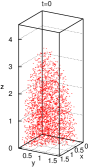
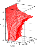
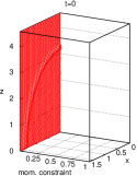
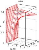
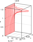
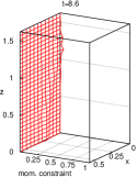
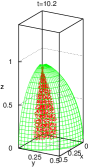
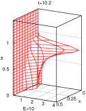
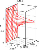
Figure 7: Snapshots of the particle distribution and the density distribution, Kretschmann curvature invariant $\mathcal{K}$ and momentum constraint violation on the $x$-$z$ plane are shown. The numerical value of every dimensionful variable is given in the unit of $M$. The peak value $\mathcal{K}_{\rm p}$ take the maximum values at $t\simeq 8.6M$. As is shown in the panel of the particle distribution at $t=10.2M$, an apparent horizon appears at this time.

The qualitative picture of the particle dynamics is similar to the previous case. However, in this case, an apparent horizon appears at $t\simeq 10.2M$ as is depicted in the lower left-most panel in Fig. 7. The value of $z$-axis at the pole of the horizon, denoted by $z_{\rm h}$ is given by $z_{\rm h}\simeq 0.82M$. The density, Kretschmann invariant and momentum constraint violation take the maximum value inside the horizon at the formation time. We show the time evolution of $\mathcal{K}_{\rm p}$ and constraint violation in Fig. 8.

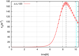
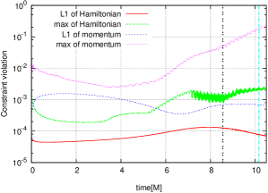
Figure 8: $\mathcal{K}_{\rm p}$ and values of constraint violation are depicted as functions of time. The vertical lines show the time at $\mathcal{K}_{\rm max}$ and the horizon formation, respectively.

From this figure, it is clear that an apparent horizon is formed after $\mathcal{K}_{\rm p}$ takes the maximum value. We also checked the resolution dependence of the shape and time at the horizon formation time. As is shown in Fig. 9, the horizon formation time and the apparent shape are almost convergent.

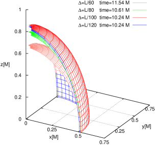
Figure 9: Resolution dependence of the horizon formation time and the apparent shape are shown.

The position of the maximum momentum constraint violation is located on the $z$-axis after $t=6M$. Let $z_{*}$ denote the value of the $z$ coordinate at the peak of the momentum constraint violation. We depict the value of $z_{*}$ as a function of time in Fig. 10.

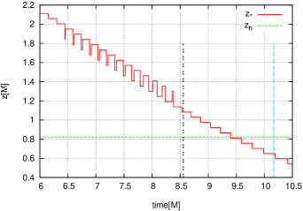
Figure 10: $z_{*}$ is depicted as a function of time. The two vertical lines show the time at $\mathcal{K}_{\rm max}$ and the horizon formation, respectively.

Although $z_{*}$ is well inside the apparent horizon at the formation time, it takes a larger value at an earlier time.

The result shown in this subsection is well understood in the sense of the hoop conjectureThorne1972 . That is, the matter distribution is too elongated for the formation of the horizon which covers the most part of the system at the moment of $\mathcal{K}_{p}=\mathcal{K}_{\rm max}$. However, after a certain period of time after $\mathcal{K}_{p}=\mathcal{K}_{\rm max}$, the matter distribution gets compacted into a region whose circumference in every direction is comparable to $4\pi M$.

IV Summary and Discussion

We have performed 3D general relativistic simulations of the non-spherical gravitational collapse of a collisionless particle system. Particles have been randomly distributed inside a prolate spheroid. Unlike the case done by Shapiro and Teukolsky (ST) in Ref. Shapiro:1991zza , exact axisymmetry has not been assumed. We have found that a peak of the Kretschmann curvature invariant appears near the pole of the matter distribution, and the peak value takes a maximum after a period of time. The maximum value of the Kretschmann curvature invariant is greater for a finer resolution and looks divergent in the limit of infinite resolution. We have also found a similar tendency for the Weyl curvature invariant. In this sense, our results also lend support to the formation of a naked singularity like in the ST case with an axially symmetric spindle collapse. It should be noted that, even if we did not find an apparent horizon, the singularity could be covered by the global event horizon. For instance, in Ref. Ponce:2010fq , such possibility is addressed for initially stationary configurations of pointlike and singular line sources. The results in Ref. Ponce:2010fq indicate the presence of a naked singularity when the size of the singular source is large enough compared with its mass. The event horizon search in the system treated in this paper is beyond the scope of this paper and we leave it as a future work.

One remarkable difference from the ST case is that the peak position of the Kretschmann invariant always stays inside the matter distribution, while it is outside the matter distribution near the pole for the ST case. The reason of this difference is not quite clear. A consistent result with ST is also reported in Ref. Yamada:2011br by Yamada and Shinkai. They performed a similar simulation to that in ST by using an axisymmetric code with a finer resolution. Therefore, the lower resolution in ST is unlikely to be the reason. One possible reason is that there is no exact axisymmetry in our case in contrast with the ST case. If it is correct, our result might suggest structural instability of the singular spacetime suggested by ST. Another difference from the ST case is that our numerical integration does not break down even when the Kretschmann invariant takes a maximum value but goes further well beyond this moment. We have not found an apparent horizon in the simulation starting from the initial situation same as in ST. As is shown in the section III.3, by using a different initial data set, we have found an example in which an apparent horizon is finally formed after a certain period of time after the occurrence of the maximum value of the peak of the Kretschmann invariant.

Not only do the analyses of collisionless particle systems make contributions to the understanding of the theoretical aspects of gravitational collapse, but also provide a model of gravitational collapse in a possible early matter-dominated phase of our Universe 1980PhLB…97..383K ; 1982SvA….26..391P ; 2009PhRvD..80f3511A ; 2012JCAP…09..017A ; 2013JCAP…05..033A . Similar analyses in cosmological situations may also make help to understand the criterion for primordial black hole formation in the matter-dominated phase Harada:2016mhb . In order to make our setting more realistic for gravitational collapse in cosmological situations, we need to choose an appropriate boundary condition (e.g., periodic boundary condition as in Refs. Yoo:2012jz ; Yoo:2013yea ) and initial data Shibata:1999zs ; Harada:2015yda . Gravitational collapse of a collisionless particle system in an expanding universe will be reported elsewhere Yoo-Harada-Okawa_prep .

Appendix A Convergence check

In this Appendix, we show a result of the convergence check for our numerical code. In Fig. 11, we plot the value of $\tilde{\gamma}_{zz}$ on $z$-axis at $t=24M$ for each resolution with the following fixed parameters:

$$\frac{L}{M}=20~{},~{}~{}\frac{b}{M}=10~{},~{}~{}e=0.9~{},~{}~{}N=125000~{},~{}~{}r_{\rm s}=2L/75.$$ (38)

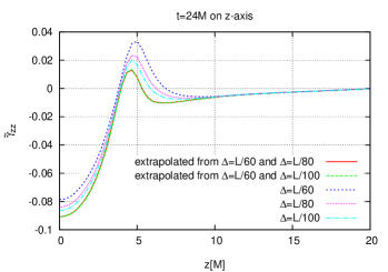
Figure 11: $\tilde{\gamma}_{zz}$ on $z$-axis at $t=24M$ is shown for each value of $\Delta$. The dependence of the second order convergence is clearly confirmed.

Assuming the second order convergence, we consider the following resolution dependence of $\tilde{\gamma}_{zz}$:

$$\tilde{\gamma}_{zz}(z;\Delta)=\tilde{\gamma}_{zz0}(z)+\tilde{\gamma}_{zz2}(z)\Delta^{2}+\mathcal{O}(\Delta^{3}),$$ (39)

where $\tilde{\gamma}_{zz0}$ and $\tilde{\gamma}_{zz2}$ represent the true value and second order error, respectively. Using $\tilde{\gamma}_{zz}$ for two different resolutions $\Delta_{1}$ and $\Delta_{2}$, we can estimate the true value $\tilde{\gamma}_{zz0}$ with the following extrapolation:

$$\tilde{\gamma}_{zz0}(z)\simeq\frac{\tilde{\gamma}_{zz}(z,\Delta_{1})\Delta_{2}^{2}-\tilde{\gamma}_{zz}(z,\Delta_{2})\Delta_{1}^{2}}{\Delta_{2}^{2}-\Delta_{1}^{2}}.$$ (40)

In Fig. 11, two different extrapolations agree with each other. This result clearly show the second order convergence of our code with fixed number and size of particles.

References

- (1) S. L. Shapiro and S. A. Teukolsky, Phys. Rev. Lett. 66, 994 (1991), Formation of naked singularities: The violation of cosmic censorship.
- (2) S. W. Hawking and G. F. R. Ellis, The Large Scale Structure of Space-TimeCambridge Monographs on Mathematical Physics (Cambridge University Press, 2011).
- (3) R. Penrose, Nuovo Cimento Rivista Serie 1 (1969), Gravitational Collapse: the Role of General Relativity.
- (4) R. Penrose, General Relativity and Gravitation 34 (2002), ”Golden Oldie”: Gravitational Collapse: The Role of General Relativity.
- (5) R. Penrose, General Relativity, an Einstein Centenary Survey (Cambridge University Press, Cambridge, England, 1979).
- (6) T. Harada and K.-i. Nakao, Phys. Rev. D70, 041501 (2004), arXiv:gr-qc/0407034, Border of spacetime.
- (7) K. S. Thorne, Magic Without Magic (Freeman, San Francisco, 1972).
- (8) Y. Yamada and H.-a. Shinkai, Phys. Rev. D83, 064006 (2011), arXiv:1102.2090, Formation of naked singularities in five-dimensional space-time.
- (9) M. Shibata, Prog. Theor. Phys. 101, 251 (1999), 3D numerical simulation of black hole formation using collisionless particles: Triplane symmetric case.
- (10) M. Shibata, Prog. Theor. Phys. 101, 1199 (1999), arXiv:gr-qc/9905058, Fully general relativistic simulation of merging binary clusters: Spatial gauge condition.
- (11) M. Shibata and T. Nakamura, Phys.Rev. D52, 5428 (1995), Evolution of three-dimensional gravitational waves: Harmonic slicing case.
- (12) T. W. Baumgarte and S. L. Shapiro, Phys.Rev. D59, 024007 (1999), arXiv:gr-qc/9810065, On the numerical integration of Einstein’s field equations.
- (13) M. Alcubierre et al., Phys. Rev. D67, 084023 (2003), arXiv:gr-qc/0206072, Gauge conditions for long term numerical black hole evolutions without excision.
- (14) H. Kreiss and J. Oliger, (1973), Methods for the approximate solution of time dependent prob- lems.
- (15) T. W. Baumgarte and S. L. Shapiro, Numerical Relativity: Solving Einstein’s Equations on the Computer (, 2010).
- (16) E. Gourgoulhon, (2007), arXiv:gr-qc/0703035, 3+1 formalism and bases of numerical relativity, Lecture notes.
- (17) M. Shibata, Numerical relativity (World Scientific Publishing Co. Pte. Ltd, Singapore, 2016).
- (18) F. H. Vincent, E. Gourgoulhon, and J. Novak, Class.Quant.Grav. 29, 245005 (2012), arXiv:1208.3927, 3+1 geodesic equation and images in numerical spacetimes.
- (19) C. W. Misner, K. S. Thorne, and J. A. Wheeler, Gravitation (W. H. Freeman, San Francisco, 1973).
- (20) S. Frittelli and O. A. Reula, Phys. Rev. Lett. 76, 4667 (1996), arXiv:gr-qc/9605005, First order symmetric hyperbolic Einstein equations with arbitrary fixed gauge.
- (21) L. E. Kidder, M. A. Scheel, and S. A. Teukolsky, Phys. Rev. D64, 064017 (2001), arXiv:gr-qc/0105031, Extending the lifetime of 3-D black hole computations with a new hyperbolic system of evolution equations.
- (22) T. Nakamura, S. L. Shapiro, and S. A. Teukolsky, Phys. Rev. D38, 2972 (1988), Naked Singularities and the Hoop Conjecture: An Analytic Exploration.
- (23) S. Chandrasekhar, Ellipsoidal figures of equilibrium (, 1969).
- (24) M. Ponce, C. Lousto, and Y. Zlochower, Class. Quant. Grav. 28, 145027 (2011), arXiv:1008.2761, Seeking for toroidal event horizons from initially stationary BH configurations.
- (25) M. Y. Khlopov and A. G. Polnarev, Physics Letters B 97, 383 (1980), Primordial black holes as a cosmological test of grand unification.
- (26) A. G. Polnarev and M. Y. Khlopov, Soviet Ast. 26, 391 (1982), Dustlike Stages in the Early Universe and Constraints on the Primordial Black-Hole Spectrum.
- (27) L. Alabidi and K. Kohri, Phys. Rev. , 063511 (2009), arXiv:0906.1398, Generating primordial black holes via hilltop-type inflation models.
- (28) L. Alabidi, K. Kohri, M. Sasaki, and Y. Sendouda, JCAP 9, 017 (2012), arXiv:1203.4663, Observable spectra of induced gravitational waves from inflation.
- (29) L. Alabidi, K. Kohri, M. Sasaki, and Y. Sendouda, JCAP 5, 033 (2013), arXiv:1303.4519, Observable induced gravitational waves from an early matter phase.
- (30) T. Harada, C.-M. Yoo, K. Kohri, K.-i. Nakao, and S. Jhingan, (2016), arXiv:1609.01588, Primordial black hole formation in the matter-dominated phase of the Universe.
- (31) C.-M. Yoo, H. Abe, K.-i. Nakao, and Y. Takamori, Phys.Rev. D86, 044027 (2012), arXiv:1204.2411, Black Hole Universe: Construction and Analysis of Initial Data.
- (32) C.-M. Yoo, H. Okawa, and K.-i. Nakao, Phys.Rev.Lett. 111, 161102 (2013), arXiv:1306.1389, Black Hole Universe: Time Evolution.
- (33) M. Shibata and M. Sasaki, Phys. Rev. D60, 084002 (1999), arXiv:gr-qc/9905064, Black hole formation in the Friedmann universe: Formulation and computation in numerical relativity.
- (34) T. Harada, C.-M. Yoo, T. Nakama, and Y. Koga, Phys. Rev. D91, 084057 (2015), arXiv:1503.03934, Cosmological long-wavelength solutions and primordial black hole formation.
- (35) C.-M. Yoo, T. Harada, and O. Hirotada, in preparation.