Active Brownian particles moving in a random Lorentz gas

Abstract

Biological microswimmers often inhabit a porous or crowded environment such as soil. In order to understand how such a complex environment influences their spreading, we numerically study non-interacting active Brownian particles (ABPs) in a two-dimensional random Lorentz gas. Close to the percolation transition in the Lorentz gas, they perform the same subdiffusive motion as ballistic and diffusive particles. However, due to their persistent motion they reach their long-time dynamics faster than passive particles and also show superdiffusive motion at intermediate times. While above the critical obstacle density $\eta_{c}$ the ABPs are trapped, their long-time diffusion below $\eta_{c}$ is strongly influenced by the propulsion speed $v_{0}$. With increasing $v_{0}$, ABPs are stuck at the obstacles for longer times. Thus, for large propulsion speed, the long-time diffusion constant decreases more strongly in a denser obstacle environment than for passive particles. This agrees with the behavior of an effective swimming velocity and persistence time, which we extract from the velocity autocorrelation function.

1 Introduction

Active matter has been in the focus of intense research for the last decade Ramaswamy2010 ; Romanczuk2012 ; Marchetti2013 ; Zottl2016 . On small length scales it describes the motion of biological microswimmers such as swimming bacteria or motile cells, and of artificial microswimmers, such as active Janus particles or self-propelled emulsion droplets Polin2009 ; Alizadehrad2015 ; Schmitt2013 ; Adhyapak2015 ; Schmitt2016 ; Maass2016 . In a homogeneous environment, microswimmers at low Reynolds number first move ballistically and then cross over to enhanced diffusion due to random rotational motion of their swimming direction Zottl2016 ; Howse2007 . Active Brownian particles provide a simple stochastic model for microswimmer such as active Janus particles Romanczuk2012 , which in contrast to bacteria do not tumble.

Natural microswimmers usually do not move in homogeneous environments but encounter soft and solid walls, obstacles Drescher2011 ; Berke2008 ; Schaar2015 ; Takagi2014 ; Kaiser2012 , or even more complex environments like the intestinal tract Berg , porous soil Ford2007 , and blood flow Engstler2007 . A heterogeneous environment can be realized in different ways, both in experiments and theory, e.g., by regular or irregular patterns of obstacles Park2008 ; Holm2011 ; Volpe2011 ; Heddergott2012 ; Majmudar2012 ; Johari2013 ; Chepizhko2013a ; Chepizhko2013 ; Reichhardt2014 ; Schirmacher2015 ; Chepizhko2015b ; Raatz2015 ; Munch2016 , mazes Khatami2016 , arrays of funnels Tailleur2009 ; Kaiser2012 ; Wan2008 ; Volpe2014 ; Galajda2007 ; Reichhardt2016 , pinning substrates Sandor2016a , or patterned light fields, which control the velocity of the microswimmer Volpe2014a ; Pototsky2013 . For a review see Zottl2016 ; Bechinger2016 .

In real systems the heterogeneities of the environment are mosty irregular. One way to model them is the random Lorentz gas Weijland1968a ; Hofling2008b ; Sch??bl2014 . In this approach the obstacles are fixed and randomly distributed with a given area fraction. The properties of the Lorenzt gas change fundamentally with varying density. In particular, it shows a transition to continuum percolation Mertens2012 , where the complementary free space stops to percolate through the whole system. As a consequence, the dynamics of a test particle in such a Lorentz gas crucially depends on density. Above a critical obstacle density, the test particle can no longer explore the whole environment but stays trapped and long-range transport is effectively suppressed. Höfling et al. have observed that in two dimensions and close to the critical density diffusive and ballistic particles show the same subdiffusive motion in a random Lorentz gas Hofling2008b ; Spanner2011 ; Bauer2010 ; Spanner2016 ; Schnyder2015 .

Microswimmers can interact in different ways with obstacles. For example, Chepizhko et al. have studied self-propelled particles in an environment of randomly distributed point-like obstacles. Instead of implementing steric interactions, they let the self-propelled particles deflect from the point-like obstacles with a characteristic turning speed Chepizhko2013a . Depending on the system parameters, this setting can lead to trapped states where particles circle around an obstacle and thus to subdiffusive motion. It also shows interesting effects during collective motion. For example, transport in the presence of obstacles is optimized by a specific noise value Chepizhko2013 ; Chepizhko2015b .

In this article we will investigate an active Brownian particle (ABP) moving in a random Lorentz gas implementing explicit steric interactions between ABP and obstacles. We will demonstrate that it performs the same subdiffusive motion as ballistic and diffusive particles close to percolation. Besides this universal feature, ABPs explore their environment faster than passive particles due to their persistent motion and therefore reach their long-time dynamics at earlier times. At intermediate times their dynamics is superdiffusive. A determining characteristic of ABPs is that they are stuck to the obstacles due to their self-propulsion. This has consequences for the diffusive spreading below the critical obstacle density. Namely, for large propulsion speed, the long-time diffusion constant decreases more strongly in a denser obstacle environment than for passive particles. We rationalize this behavior by studying the velocity autocorrelaton function, which motivates us to introduce an effective swimming velocity and persistence time.

The article is structured as follows. In sect. 2 we introduce the equations of motion of the ABP and model the obstacle environment as a random Lorentz gas. In sect. 3 we recap the dynamics of a passive Brownian particle in the Lorentz gas and compare it to the ABP in sect. 4. Finally, in sect. 5 we discuss how the long-time diffusion coefficient of an ABP and its persistent motion is reduced in the presence of obstacles using the velocity autocorrelation function. We finish with concluding remarks in sect. 6.

2 Introduction of the model

2.1 Active Brownian particle interacting with obstacles

Our model of a microswimmer is a circular active Brownian particle (ABP) with radius $R_{s}$. It moves with a constant velocity $v_{0}$ along a direction ${\mathbf{e}}$ in a two-dimensional environment filled with circular obstacles of radius $R_{o}$. The particle also experiences rotational and translational thermal noise. Thus, the Langevin equations governing the dynamics of the ABP reads Romanczuk2012 ; Zottl2016

$$\begin{split}\frac{\mathrm{d}\mathbf{r}(t)}{\mathrm{d}t}&=v_{0}\mathbf{e}(t)+\mu^{T}\sum_{i}\mathbf{F}_{o}^{i}+\sqrt{2D^{T}}\boldsymbol{\eta}^{T}(t),\\ \frac{\mathrm{d}\mathbf{e}(t)}{\mathrm{d}t}&=\sqrt{2D^{R}}\boldsymbol{\eta}^{R}(t)\times\mathbf{e}(t)\,,\end{split}$$ (1)

where $D^{T}$ and $D^{R}$ are the respective translational and rotational diffusion constants. Furthermore, $\boldsymbol{\eta}^{T}(t)$ is a rescaled stochastic force and $\boldsymbol{\eta}^{R}(t)$ a rescaled stochastic torque, both with zero mean and Gaussian white noise correlations:

$$\langle\boldsymbol{\eta}^{T,R}(t)\rangle =0,$$ (2)

$$\langle\boldsymbol{\eta}^{T,R}(t_{1})\otimes\boldsymbol{\eta}^{T,R}(t_{2})\rangle =\mathbf{1}\delta(t_{1}-t_{2}).$$ (3)

Note that the stochastic torque always points out of the $x,y$ plane, $\boldsymbol{\eta}^{R}=\eta_{z}^{R}\mathbf{e}_{z}$.

Finally, the interaction force $\mathbf{F}_{o}^{i}$ between an ABP and obstacle $i$ is modeled by pure volume exclusion. It derives from the Weeks-Chandler-Anderson potential, which is a Lennard-Jones potential cut off at the minimum:

$$V=\begin{cases}4\varepsilon\left[\left(\frac{\sigma}{r}\right)^{12}-\left(\frac{\sigma}{r}\right)^{6}\right]+\varepsilon&\text{for }r<d^{*}\\ 0&\text{for }r\geq d^{*}\,.\end{cases}$$ (4)

Here, $d^{*}=2^{1/6}\sigma=R_{s}+R_{o}$ is the distance, where the potential is minimal and where it also vanishes. The resulting force in Eq. (1) is then given by $\mathbf{F}_{o}=-\boldsymbol{\nabla}V$. Hydrodynamic interactions are neglected in this model.

The motion of the active Brownian particle in free space is fully characterized by the dimensionless Péclet number, which compares the times needed for diffusive and active motion along a distance $R_{s}$,

$$\text{Pe}=\frac{2R_{s}v_{0}}{D^{T}}\,.$$ (5)

Moreover, in a homogeneous bulk system the ABP moves ballistically on the persistence length $\Delta s_{r}=v_{0}\tau_{r}$, where $\tau_{r}=1/D^{R}$ is the persistence time completely determined by the rotational diffusion constant.

2.2 Lorentz model and continuum percolation

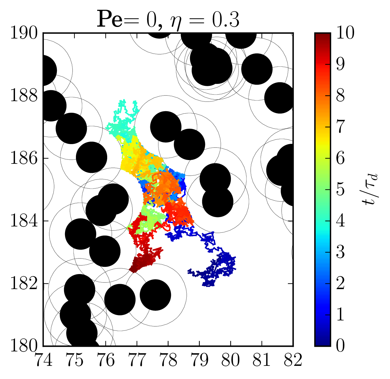
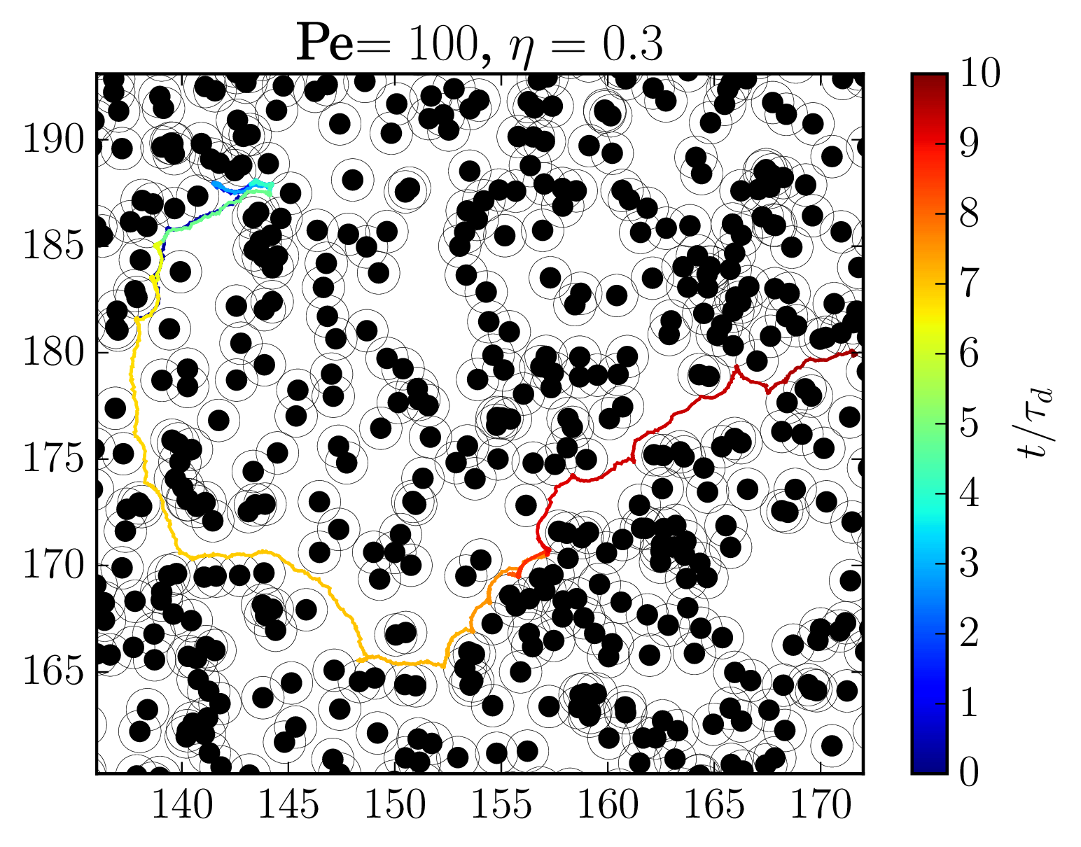
Figure 1: Left: Trajectory of a passive Brownian particle in a heterogeneous environment with reduced obstacle density $\eta=0.3$. Right: Trajectory of an ABP with $\mathrm{Pe}=100$ under the same conditions. Time along the trajectories is encoded by color according to the color bar.

We model the heterogeneous environment by a random Lorentz gas, where circular obstacles are randomly distributed in the plane and with positions fixed in space (spatial Poisson point process) Stauffer1994 . The obstacles are assigned a reduced density or area fraction $\eta=\pi R_{o}^{2}/A$, where $A$ is the area of the system. However, since the obstacles can fully penetrate each other, the actual area fraction is Torquato2002

$$\phi_{o}=1-e^{-\eta}\,.$$ (6)

Percolation theory gives some first insights how an ABP moves through the random Lorentz gas. It provides a critical density for the transition to an infinite cluster of overlapping disks percolating through the whole system Torquato2002 or for the percolating free space between obstacles Bauer2010 . In two dimensions the critical particle area fraction for the percolating cluster of connected disks is $\phi_{o,c}=0.67637\pm 0.00005$ Torquato2002 , while the critical void area fraction for the percolating free space is $\phi_{v,c}\approx 0.324$ Bauer2010 . The latter determines whether the ABP ultimately performs diffusive motion or becomes localized (localization transition). In two dimensions the two area fractions add up to one, because the percolating clusters of free space and of overlapping disks are complementary to each other. They can only coexist in strongly anisotropic systems but not in the random Lorentz gas with its isotropic distribution of disks. In three dimensions this restriction is no longer valid.

In our simulations we always choose the reduced density $\eta$ instead of the actual area fraction $\phi_{o}$. Using Eq. (6) the critical value of the reduced obstacle density is $\eta_{c}=-\ln\left(1-\phi_{o,c}\right)\approx 1.12815$. Now, the ABP itself has a finite extent, so the accessible space for its center of mass is determined not only by the obstacles but also by the swimmer radius. The ABPs can only pass between two obstacles if their distance is larger than $2(R_{o}+R_{s})$ assuming ideal hard-core interactions. Thus, we can map the problem of an extended swimmer in a random environment onto a point-like swimmer in an environment of obstacles with an effective radius $R_{\text{eff}}=R_{o}+R_{s}=2R_{o}$ and an effective reduced density $\eta^{\text{eff}}=N\pi(R_{\text{eff}})^{2}/V=4\eta$ (here and in the following we assume $R_{o}=R_{s}$). Therefore, we find for the critical reduced density of the actual obstacles

$$\eta_{c}=\eta_{c}^{\text{eff}}/4\approx 0.28\,.$$ (7)

We will see that in our system the localization transition takes place at densities larger than the theoretically predicted value $\eta_{c}\approx 0.28$. This is mainly due to a finite-size effect. Near to the critical density, the size of the largest finite cluster of free space (or the largest trap) diverges as the correlation length: $\xi\sim|\eta-\eta_{c}|^{-\nu}$. The exponent $\nu=4/3$ is known from lattice percolation and also valid for continuum percolation. In our simulations we can only realize a finite system with size $L$ and apply periodic boundary conditions, in order to mimic infinite systems. The system size $L$ is then an upper bound for the size of the largest cluster of accessible space given by $\xi$. Coming from high densities $\eta$, the free space starts to percolate for $\xi\approx L$ and the apparent critical density in a finite system is shifted according to $\eta_{c}(L)-\eta_{c}(\infty)\sim L^{-1/\nu}$. In contrast to Ref. Bauer2010 , where the system size was $L/R_{o}=10000$, we use much smaller systems with a fixed number of $15000$ obstacles. Depending on $\eta$, the system size becomes $L=\sqrt{A}=\sqrt{15000\pi R_{o}^{2}/\eta}$, which ranges from 140 to 343 for $\eta\in[0.1,0.6]$ used in our simulations. This is a factor 100 smaller than in Bauer2010 and roughly gives a shift of $\eta_{c}(L)-\eta_{c}(\infty)\sim 0.02$, in agreement with our results presented below. Finally, note that in contrast to typical studies of percolation, we keep the number of obstacles fixed rather than the system size. This makes sense since active particles strongly accumulate at bounding surfaces which, therefore, strongly influence the dynamics of ABPs Schaar2015 .

2.3 System parameters

For all of our simulations we use an environment with 15000 obstacles. To determine the long-time behavior of the ABPs, we perform simulations with 500 non-interacting swimmers in the same environment. In order to study the short-time behavior and especially the velocity autocorrelation function in more detail, we simulate 100 non-interacting swimmers in upto six different realizations of the environment, so 600 trajectories in total.

We randomly place the obstacles on a square with area $A$ and allow them to overlap. Then, the swimmers are randomly distributed but overlaps with obstacles are not allowed. If they occur, the relevant swimmers are newly placed. Since ABPs eventually accumulate at the surfaces of the obstacles, the random swimmer distribution is not the steady state of the system. So, before we start our data acquisition, we let the system equilibrate during a time $0.5\tau_{d}$. Here,

$$\tau_{d}=(2R_{s})^{2}/D^{T}$$ (8)

is the time a passive particle needs to diffuse its own size, while the ABP moves over much longer distances during $\tau_{d}$ depending on the Péclet number.

In the following, we set $R_{s}=R_{o}=R$. We give lengths in units of $2R$ and rescale time by $\tau_{d}=(2R)^{2}/D^{T}$. In three dimensions the respective thermal diffusion coefficients for translation and rotation are related by $D^{R}=3D^{T}/(4R^{2})$ Zottl2016 . Albeit in two dimensions, we use the same ratio in all our simulations and the ratio of the diffusion times becomes $\tau_{r}/\tau_{d}=1/3$. Finally, for the time step $\Delta t$ in the Langevin-dynamics simulations we choose $\Delta t\leq 10^{-5}$ in units of $\tau_{d}$, where we need to adjust $\Delta t$ to smaller values with increasing Péclet number.

3 Influence of the random environment on a passive Brownian particle

Before presenting our results for ABPs, we review some basic results for passive Brownian particles. Figure 1 shows a close-up of the system with obstacles in black. The surrounding excluded volume due to the finite size of the Brownian particles is indicated by gray rings. We show the trajectories of the passive and active Brownian particles, where color encodes time. The trajectory of the center of the passive particle (left) is only governed by diffusion. It explores the accessible free space and moves about eight particle diameters away from the starting point as expected for $t=10$.

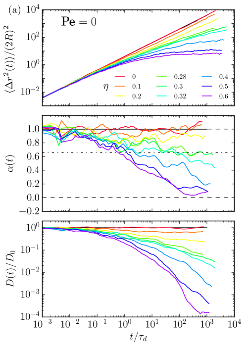
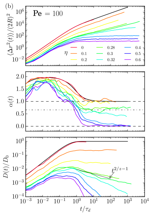
Figure 2: Mean squared displacement $\langle\Delta r^{2}\rangle$ (top), local exponent $\alpha(t)$ (center), and local diffusion coefficient $D(t)/D_{0}$ (bottom) for (a) a passive and (b) an active Brownian particle. The dashed-dotted lines in the middle graphs indicate $\alpha=2/z\approx 0.66$.

To be more quantitative, we discuss the mean squared displacement, the local exponent $\alpha(t)$, and the local diffusion coefficient $D(t)$ for different reduced obstacle densities as shown in Fig. 2(a).

3.1 Mean squared displacement

For a Brownian particle in two dimensions, diffusing in free space, the mean squared displacement is given by $\langle\Delta r^{2}(t)\rangle=4D^{T}t$ and shown by the black curve in the upper graph of Fig. 2(a). At small obstacle densities ($\eta=0.1$, 0.2) the mean squared displacement behaves similar to the free case, however, with a smaller diffusion coefficient (note the double-logarithmic plot). For very high obstacle densities ($\eta=0.5$, 0.6) it eventually saturates at finite values. At intermediate obstacle densities we observe subdiffusive behavior also at long times. Thus, the mean squared displacement shows a transition from a linear to a localized regime via subdiffusion. In an inifinitely extended system, the latter occurs exactly at the critical density $\eta_{c}$, where the free space does not percolate any more. Beyond this density particles are trapped in regions of finite size and the mean squared displacement saturates at $\langle\Delta r^{2}(t)\rangle$ equal to the areas of these regions. All this is thoroughly reviewed in Ref. Bauer2010 . We will now be more quantitative to be able to compare with the ABPs.

3.2 Local exponent

Subdiffusive behavior is indicated by $\langle\Delta r^{2}(t)\rangle\propto t^{\alpha}$ with an exponent $\alpha<1$. Thus we determine the local exponent

$$\alpha(t)=\frac{\mathrm{d}\log\langle\Delta r^{2}(t)\rangle}{\mathrm{d}\log t}\,.$$ (9)

from the mean squared displacement and plot it in the middle graph of Fig. 2(a). In free space ($\eta=0$) $\alpha(t)$ does not change in time and is always one. Also for low $\eta$ the exponent fluctuates around one, which indicates that the particle dynamics is still governed by conventional diffusion and the obstacles do not have much impact, whereas for very high $\eta$ the exponent tends to zero as expected when particles become trapped or localized. For intermediate obstacle densities $\eta$ the local exponent $\alpha(t)$ is smaller than one and indicates subdiffusive behavior. In particular, at $\eta=0.28$ the exponent reaches the value $\alpha=2/z=2/3.036\approx 0.66$ as expected at the percolation transition and shown by the dashed-dotted line. However, for most parameters the exponent has not yet reached a stationary value.

In an inifinite system close to percolation, particles exhibit subdiffusion below the correlation length $\xi$ of the fractal cluster of free space. Then, on lengths larger than $\xi$ they either become trapped ($\eta<\eta_{c}$) or diffusive ($\eta>\eta_{c}$) Torquato2002 . Subdiffusion persists exactly at $\eta=\eta_{c}$, where $\xi$ diverges. In finite systems the correlation length $\xi$ is bounded by the system size $L$. So any subdiffusive motion at short times with $\langle\Delta r^{2}(t)\rangle<\xi^{2}$ is only transient and will ultimately become trapped for $\eta\geq\eta_{c}(L)$ with an exponent $\alpha=0$ or turn into normal diffusion for $\eta<\eta_{c}$ with an exponent $\alpha=1$. Thus, in Fig. 2(a), middle graph the curve for $\eta=0.28$ and probably also for $\eta=0.3$ will ultimately reach one for long times beyond our simulated times, whereas the curves for larger $\eta$ clearly tend towards zero.

Passive particles diffuse slowly and in contrast to active particles need a long time to explore their environment. Together with the diverging $\xi$ close to the percolation transition, this explains why in Fig. 2 only the exponents far from the critical density ($\eta=0.1,02$ and $\eta=0.6$) have reached the stationary values of one and zero, respectively.

3.3 Local diffusion coefficient

Another quantity to characterize the mean squared displacement is the local diffusion coefficient

$$D(t)=\frac{1}{4}\frac{\mathrm{d}\langle\Delta r^{2}(t)\rangle}{\mathrm{d}t}\,.$$ (10)

In the lower graph of Fig. 2(a) we plot it normalized by the diffusion coefficient in free space, $D_{0}$, which is $D^{T}$ for passive particles. Already at low densities $\eta$ the diffusion coefficient $D(t)$ is not constant in time. At $\eta=0.1$ it slightly decreases and around $t=\tau_{d}$ saturates at a ratio $D(t)/D_{0}$ below one. For $\eta=0.2$ the ratio decreases further and takes more time to become stationary. For obstacle densities above the percolation transition $D(t)$ tends to zero as expected. In agreement with the discussion in Sec. 3.2, at intermediate densities the time to reach a diffusive state with a constant $D(t)$ or a localized state with $D(t)=0$ becomes very large close to the critical density $\eta=\eta_{c}(L)$.

Analyzing the local exponent $\alpha(t)$ and the local diffusion coefficient $D(t)/D_{0}$ shows that obstacles at low densities $\eta$ act as an additional source of noise, while at high obstacle densities $\eta$ they confine the available space of the swimmers to a finite extent. A good discussion of the scaling behavior of the dynamics of Brownian particles in a heterogeneous environment close to percolation is found in Bauer2010 .

4 Influence of the random environment on a microswimmer

In this section we first study how the complex environment influences the motion of ABPs moving at $\mathrm{Pe}=100$, as an example. We show how the dynamics of the swimmer changes with obstacle density. The results to be discussed below are plotted in Fig. 2(b). In sect. 4.4 we will compare ABPs of different velocities close to the percolation transition.

In contrast to a passive particle the ABP is much more in contact with the obstacles and covers a longer path due to its swimming velocity. This is demonstrated in Fig. 1(b) for an example trajectory at $\mathrm{Pe}=100$. The ABP spends less time in the free space but is rather guided along the walls of obstacle clusters. Due to its overdamped motion the ABP just stops if its self-propulsive velocity points perpendicular to a bounding wall. However, as long as the swimming direction has a component parallel to an obstacle surface, it will slide along the surface. The ABP leaves the obstacle due to rotational diffusion of its swimming direction (governed by the persistence time $\tau_{r}$) and because the obstacle is curved.

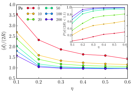
Figure 3: Mean distance of an ABP to the closest obstacle, $\langle d\rangle/(2R)$, plotted versus $\eta$ for different $\mathrm{Pe}$. Inset: Probability for the ABP to have a distance $d$ smaller than $1.1(2R)$ to the nearest obstacle, $P(d/(2R)<1.1)$.

Indeed, Fig. 3 demonstrates that the mean distance of an ABP to the closest obstacle drastically decreases with increasing Péclet number at the same obstacle density $\eta$. In partiular, for $\mathrm{Pe}\geq 50$ the mean distance is close to $2R$. It varies only little with increasing $\eta$ and all ABPs reside close to or at obstacle surfaces. Correspondingly, the probability of an ABP to be at a distance smaller than $1.1(2R)$ to the nearest obstacle increases with $\mathrm{Pe}$ and approaches one (see inset of Fig. 3).

4.1 Mean squared displacement

Free space

For an ABP moving with velocity $v_{0}$ the mean squared displacement in free space can be written as Howse2007 ; Downton2009 ; TenHagen2011 :

$$\langle\Delta r^{2}(t)\rangle=4D^{T}t+2v_{0}^{2}\tau_{r}t-2v_{0}^{2}\tau_{r}^{2}\left(1-e^{-t/\tau_{r}}\right).$$ (11)

From this equation one infers two relevant time scales and an effective diffusion coefficient at long times. On times shorter than

$$\tau_{1}=4D^{T}/v_{0}^{2}=4\tau_{d}/\mathrm{Pe}^{2}\,,$$ (12)

where we used Eqs. (5) and (8) to derive the second expression, translational diffusion dominates over active propulsion and the ABPs move by thermal diffusion. Typically, this regime is only observed at small Péclet numbers. On times up to the persistence time $\tau_{r}=1/D^{R}$ (in two dimensions), self-propulsion dominates and the ABPs move ballistically. On times larger than $\tau_{r}$ the particle orientation decorrelates and diffusive motion occurs with an increased effective diffusion coefficient $D_{\text{eff}}=D^{T}+1/2v_{0}^{2}\tau_{r}$. The ballistic regime and the crossover to enhanced diffusion around $\tau_{r}=\tau_{d}/3$ is clearly illustrated in the upper graph of Fig. 2(b). The initial diffusive regime occurs at times smaller than $\tau_{1}=4\cdot 10^{-4}\tau_{d}$ and is not visible in the graph.

Random environment

Here the mean squared displacement in Fig. 2(b) follows the general trend set by passive particles and ABPs in free space. An inital ballistic or superdiffusive regime is followed by either effective diffusion at small densities $\eta$ or a localization at high $\eta$, where $\langle\Delta r^{2}(t)\rangle$ saturates at the square of the mean trap size. Close to the critical percolation density we now observe a subdiffusive regime, which extends over several decades in time compared to the passive case. The time spent in the subdiffusive regime becomes shorter further away from the critical density (see for example $\eta=0.4$).

Due to their self-propulsion, ABPs cover a much longer distance than passive particles in the same time (see Fig. 1). As a result, they explore the confining space of a trap much faster. Thus, the mean squared displacement of ABPs at densities $\eta=0.4$ and higher saturates at a pronounced plateau much earlier than for passive particles.

At short times, passive particles or slow swimmers explore the whole free space by diffusion with the same diffusion coefficient. Therefore, all the curves for different $\eta$ in the upper graph of Fig. 2(a) initially lie on top of each other. In contrast, for fast ABPs the inital ballistic/superdiffusive motion slows down with increasing $\eta$. ABPs strongly accumulate at the obstacles and the time they spend in free space decreases with $\eta$. Thus, effectively also their mean motility decreases with increasing $\eta$ at short times, which explains that the mean squared displacement in Fig. 2(b) is shifted downwards. In sect. 5.2 we will introduce an effective swimming velocity, which rationalizes the observed behavior.

4.2 Local exponent

Free space

In the middle graph of Fig. 2(b) the black solid line shows the analytic result for the local exponent of an ABP moving in free space, which we directly calculate using Eq. (11):

$$\alpha(t)=\frac{\mathrm{d}\log\langle\Delta r^{2}\rangle}{\mathrm{d}\log t}=\frac{4D^{T}t+2v_{0}^{2}\tau_{r}t-2v_{0}^{2}\tau_{r}te^{-t/\tau_{r}}}{\langle\Delta r^{2}\rangle}\,.$$ (13)

Rescaling times by $\tau_{d}$ and lengths by the diameter $2R$, one shows that the temporal evolution of the local exponent only depends on the Péclet number, which also sets the time scale for the transition from diffusion to ballistic movement, as $\tau_{1}$ in Eq. (12) demonstrates. The second time scale $\tau_{d}$ marks the transition from ballistic back to diffusive motion.

Random environment

In contrast to passive particles, the ABPs reach their long-time behavior much faster at times around $\tau_{d}$ and the transition is more pronounced. This is clearly demonstrated by the graphs for $\alpha(t)$ in Fig. 2. The exponent of the ABP assumes $\alpha=1$ for the diffusive motion at small $\eta=0.1,0.2$, becomes zero at high obstacle densities $\eta=0.4,0.5,0.6$, and indicates clear subdiffusive motion at the intermediate densities $\eta=0.28,0.3$. As for passive particles we roughly find $\alpha$ close to 0.66 (dashed-dotted line) indicating that subdiffusion close to the critical percolation density is mainly governed by the topology of free space and not by the difference between Brownian and ballistic active motion.

At short times the ballistic/superdiffusive regime shrinks in the presence of obstacles with increasing $\eta$ and also the local exponent $\alpha$ decreases. In particular, the crossover time from ballistic/superdiffusive motion to diffusion shifts to smaller times when $\eta$ becomes larger. Interestingly, at high obstacle densities, $\eta\geq 0.4$, a short diffusive regime with $\alpha=1$ is established before localization with $\alpha=0$. occurs.

4.3 Local diffusion coefficient

Free space

We readily calculate the local diffusion coeffcient of an ABP using Eq. (11):

$$D(t)=\frac{1}{4}\frac{\mathrm{d}\langle\Delta r^{2}(t)\rangle}{\mathrm{d}t}=D^{T}+\frac{1}{2}v_{0}^{2}\tau_{r}-\frac{1}{2}v_{0}\tau_{r}e^{-t/\tau_{r}}\,.$$ (14)

It is plotted as the solid black line in the bottom graph of Fig. 2 and shows a plateau at the effective diffusion coefficient $D_{\text{eff}}=D^{T}+v_{0}^{2}\tau_{r}/2$, as already discussed.

Random environment

Very prominently, at low $\eta$ the steady-state diffusion coefficient strongly decreases from the free-space value. Thus, even at low densities, the obstacles have a much more pronounced effect compared to passive particles and strongly decrease the mobility of ABPs. For high obstacle densities, $\eta\geq 0.4$, one clearly observes how $D(t)$ approaches zero. This occurs at smaller times, when $\eta$ increases. Finally, in the vicinity of the percolation transition the diffusion coefficient behaves close to the universal power law, $D(t)\propto t^{2/z-1}$, as indicated in the graph.

4.4 Microswimmers in a random Lorentz gas close to the percolation transition

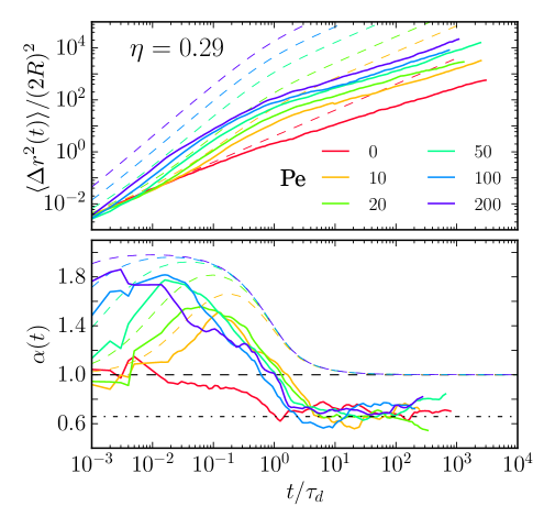
Figure 4: Mean squared displacement $\langle\Delta r^{2}\rangle$ (top) and local exponent $\alpha(t)$ (bottom) for ABPs plotted versus time for different Péclet numbers at $\eta=0.29$. The dashed lines show the analytic results for free space from Eqs. (11) and (13). The dashed-dotted line in the bottom graph indicates $\alpha=2/z\approx 0.66$.

In this section we study how ABPs move in a two-dimensional random environment close to the percolation transition. Investigations of passive particles, both diffusive and ballistic, demonstrate some universal behavior Bauer2010 . In Fig. 4 we plot the mean squared displacement $\langle\Delta r^{2}(t)\rangle$ and the local exponent $\alpha(t)$ for ABPs moving with different Péclet numbers in an environment with $\eta=0.29$. For comparison, the dashed lines show the analytic results for free space without any obstacles from Eqs. (11) and (13).

Two features are visible. First, while in free space the curves for the mean squared displacement are shifted upwards with increasing $\mathrm{Pe}$, in the presence of the obstacles they roughly emanate from the same value at the smallest time $t=10^{-3}\tau_{d}$. The reason is that ABPs assemble at and swim against the obstacles as discussed in the beginning of Sec. 4. So, in contrast to free space only a small fraction of them can move forward when rotational diffusion orients their swimming directions away from the obstacles. In Sec. 5.2 we will rationalize this behavior by introducing an effective swimming velocity $v_{\mathrm{eff}}$.

Second, while in free space the ABPs enter the diffusive regime for $t>\tau_{d}$, they all show subdiffusive motion in the random environment close to the percolation transition. For intermediate times $1<t/\tau_{d}<10^{2}$ and for all Péclet numbers the exponent $\alpha$ stays close to the universal value $\alpha\approx 0.66$ shown by the dashed-dotted horizontal line in the lower plot. This indicates that close to the percolation transition the dynamics of the ABP is entirely controlled by the random environment regardless of $\mathrm{Pe}$. One can expect such a behavior from the results of Refs. Bauer2010 ; Spanner2016 . For the same random environment they showed that in two dimensions the transport of passive particles, either Brownian or ballistic, shares the same universality class.

5 Long-time diffusion and persistent motion

We now discuss two overall features of ABPs moving in a random Lorentz gas. First, we look at the long-time diffusion coefficient for densities below the percolation transition and then address how the persistent motion of an ABP is reduced in the presence of obstacles using the velocity autocorrelation function.

5.1 Long-time diffusion coefficient

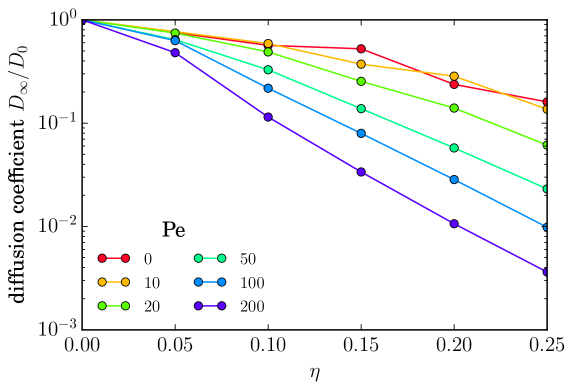
Figure 5: Long-time diffusion coefficient $D_{\infty}$ versus $\eta$ for different $\mathrm{Pe}$. $D_{0}$ is the coefficient for $\eta=0$.

Below the percolation threshold, the local diffusion constant $D(t)$, which we determine from the mean squared displacement using Eq. (10), assumes a constant value $D_{\infty}$ in the limit of long times. In Fig. 5 we plot $D_{\infty}$ versus $\eta$ for different $\mathrm{Pe}$ and refer it to the respective free-space value $D_{0}(\eta=0)$. All $D_{\infty}$ decrease with increasing obstacle density, however the decrease is stronger for larger Péclet numbers. While for passive particles the diffusion coefficient declines by less than an order of magnitude, it decreases by more than two orders for $\mathrm{Pe}=200$. The reason is that at such a high Péclet number the ABP is mostly stuck at the obstacles and hardly explores the space in between. This can be rationalized by an effective swimmining speed smaller than the free-space value $v_{0}$, which we introduce in the following.

5.2 Velocity autocorrelation function

The velocity autocorrelation function (VACF) is a means to demonstrate the persistent motion of microswimmers. Therefore, we study now how the VACF changes for ABPs in the random Lorentz gas, in order to extract effective values for swimming velocitiy, decorrelation time, and persistence length.

Free space

In free space the velocity autocorrelation function $C_{0}(t)=\langle\mathbf{v}(t)\cdot\mathbf{v}(0)\rangle$ follows from the Langevin equation (1) setting $\mathbf{F}_{o}^{i}=\mathbf{0}$. With $\dot{\mathbf{r}}=\mathbf{v}$ and the properties of Gaussian white noise as defined in Eqs. (2) and (3), the VACF becomes Kapral2013

$$C_{0}(t)=\langle\mathbf{v}(t)\cdot\mathbf{v}(0)\rangle=v_{0}^{2}\langle\mathbf{e}(t)\cdot\mathbf{e}(0)\rangle+2D^{T}\delta(t)$$ (15)

with the orientational correlation function Dhont1996

$$\langle\mathbf{e}(t)\cdot\mathbf{e}(0)\rangle=e^{-t/\tau_{r}}\,.$$ (16)

The decorrelation time in two dimensions is $\tau_{r}=1/D^{R}$. In the following we will also call it persistent time, since it gives the time scale on which the ABP moves persistently in one direction. Note, in the absence of external forces, the deterministic velocity of the ABP always points along the orientation vector $\mathbf{e}(t)$, therefore $C_{0}(t)$ is determined by the autocorrelations of $\mathbf{e}(t)$.

Random environment

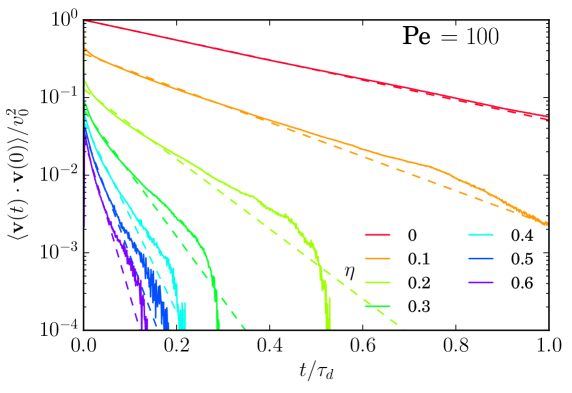
Figure 6: Velocity autocorrelation functions for $\mathrm{Pe}=100$ and different obstacle densities. The dashed lines indicate the exponential fit from Eq. (17).

In a random Lorentz gas an ABP interacts sterically with the obstacles, where it cannot move along its orientation vector $\mathbf{e}(t)$. It rather slides along the boundaries of the obstacles or is stuck in traps with convex shape formed by the obstacles. Both cases are illustrated in Fig. 1. Because we do not take into account hydrodynamic interactions with the obstacles and there are no other torques acting, the dynamics of the orientation vector $\mathbf{e}(t)$ is not affected by the random environment. Thus, its autocorrelation function follows Eq. (16). However, the full VACF strongly depends on the steric interactions of the ABP with the obstacles and cannot be calculated analytically. Therefore, we determine it from the swimmer trajectories. We calculate velocity values at discrete timesteps [$\mathbf{v}(t)=\Delta\mathbf{r}(t)/\Delta t$], numerically compute the Fourier transform of the time series, and then the VACF as $C(t)=\int\langle|\mathbf{v}(\omega)|^{2}\rangle e^{i\omega t}d\omega/(2\pi)$ using the Wiener-Khinchin theorem Kubo1991 .

As an example, Fig. 6 shows $C(t)=\langle\mathbf{v}(t)\cdot\mathbf{v}(0)\rangle$ in units of $v_{0}2$ for $\mathrm{Pe}=100$ for different obstacle densities $\eta$. While at $\eta=0$ we nicely recover the expected exponential decay from the orientational decorrelation, we observe deviations from it with increasing $\eta$. The autocorrelations in velocity decay faster with increasing $\eta$ and then drop sharply to zero. At times much smaller than $\tau_{d}$ we can even see anticorrelations in $C(t)$ (not shown). They arise at times $t\leq\tau_{1}=4\tau_{d}/\mathrm{Pe}^{2}$, where thermal translational diffusion dominates over active propulsion [see Eq. (12)]. While stuck at an obstacle and oriented towards it, Brownian motion moves the ABP away from the obstacle and thereby causes these anticorrelations.

Approximating the VACF by an exponential,

$$C(t)=v_{\text{eff}}^{2}e^{-t/\tau_{\text{eff}}}\,,$$ (17)

allows us to define an effective propulsion velocity $v_{\text{eff}}$ and an effective persistence time $\tau_{\text{eff}}$. The velocity $v_{\text{eff}}$ can be interpreted as the mean velocity of an ABP in the crowded environment. It is smaller than $v_{0}$, since the VACF also averages over ABPs, which are stuck at obstacles or in traps. The exponential curves determined by least square fits for the VACF data in the range $0.01\tau_{d}<t<\tau_{d}$ are shown as dashed lines in Fig. 6.

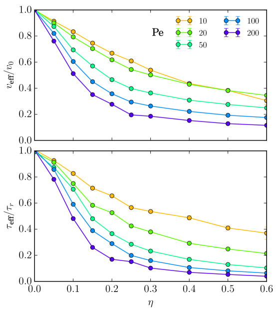
Figure 7: Effective propulsion velocity $v_{\text{eff}}$ in units of $v_{0}$ (top) and effective persistence time $\tau_{\text{eff}}$ in units of $\tau_{r}$ (bottom) plotted versus $\eta$ for different Péclet numbers.

In Fig. 7 we show the fit parameters $v_{\text{eff}}$ (top) and $\tau_{\text{eff}}$ (bottom) rescaled, respectively, by the intrinsic propulsion velocity $v_{0}$ and the orientational decorrelation time $\tau_{r}$. The effective velocity decreases with increasing $\eta$ since the ABP has less free space to move forward and thus the probability to find it at an obstacle with zero or reduced velocity increases. The same is true for larger $\mathrm{Pe}$, where the ABP traverses the free space faster and thereby spends more time being stuck at the obstacles. The persistence time $\tau_{\text{eff}}$, on which velocity correlations decay, shows the same behavior. It decreases with increasing $\eta$ and $\mathrm{Pe}$, thus when the ABP spends more time at the obstacles, where its total velocity changes magnitude and direction.

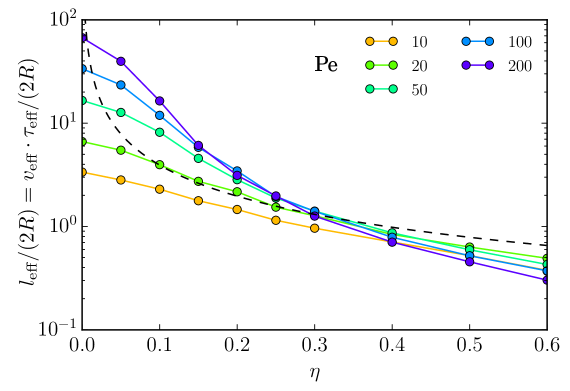
Figure 8: Effective persistence length $l_{\text{eff}}=v_{\text{eff}}\cdot\tau_{\text{eff}}$ in units of obstacle diameter $2R$ plotted versus $\eta$ for different $\mathrm{Pe}$. The black dashed line corresponds to the mean free path $l_{\text{free}}$ in a random Lorentz gas.

It is instructive to introduce an effective persistence length $l_{\text{eff}}=\tau_{\text{eff}}\cdot v_{\text{eff}}$, which we plot in units of obstacle diameter $2R$ in Fig. 8. At $\eta=0$, $l_{\text{eff}}$ coincides of course with the persistence length of an ABP in free space, $v_{0}\tau_{r}$. It decreases with increasing $\eta$ but below $\eta=0.3$ it rises with $\mathrm{Pe}$, which makes sense. However, for sufficiently large $\eta$ we expect $l_{\text{eff}}$ to be governed by the random environment of the Lorentz gas, for which the mean free path is $l_{\text{free}}=(RN/L^{2})^{-1}=\pi R/4\eta$ Torquato2002 . It is plotted as black dashed line in Fig. 8. Indeed, at around $\eta=0.3$, i.e., above the percolation density $\eta_{c}\approx 0.28$, the effective persistence lengths for different $\mathrm{Pe}$ are close to $l_{\text{free}}$, except for $\mathrm{Pe}=10$, where translational Brownian motion is still important. Above $\eta=0.3$ they all lie below the geometrical length $l_{\text{free}}$ and are smallest for the largest $\mathrm{Pe}$, as expected from the definition of $l_{\text{eff}}$.

6 Summary and conclusions

To conclude, in this article we studied the dynamics of active Brownian particles in a two-dimensional heterogeneous environment of fixed obstacles modeled by a random Lorentz gas. Using Brownian dynamics simulations, we explored how ABPs with different Péclet numbers move at varying obstacle density. The percolation transition of the Lorentz gas plays a major role for the long-time dynamics of ABPs, separating long-range transport of ABPs on the one hand from trapping of ABPs on the other hand. At obstacle densities below the critical density, ABPs are able to diffuse over long distances, while at obstacle densities above the critical density all ABPs are trapped in finite regions. This separation is independent of the Péclet number of the ABPs.

Close to the critical obstacle density, we observe that independent of the Péclet number, ABPs show subdiffusive motion on intermediate time scales with the same dynamic exponent as passive and ballistic particles. Thus, we expect that in two dimensions they share the same universality class with passive diffusive and ballistic particles. Therefore, the properties of the random Lorentz gas alone control the transition between long-range transport and trapping of ABPs as well as the dynamic exponent at and close to the percolation transition. However, in contrast to this universal behavior, we find that ABPs due to their persistent motion explore their environment faster than passive particles and, consequently, reach their long-time dynamics at earlier times. The persistent motion also makes ABPs superdiffusive on intermediate times.

A main characteristic of ABPs is that they swim against obstacles and are stuck there until noise rotates them away from the surface normal. As a result, the long-time diffusion constant decreases more strongly in a denser obstacle environment than for passive particles and this effect becomes stronger for large Péclet numbers. For example, for ABPs with $\mathrm{Pe}=200$ the diffusion constant decreases by more than two orders of magnitude until an obstacle density of 0.25, while the decline for passive particles is below a factor of ten.

Diffusion of ABPs in free space is determined by propulsion velocity and persistence time, while in a random environment obstacles perturb the persistent motion of ABPs even at low densities. By measuring the velocity autocorrelation functions from the trajectories of the ABPs and making an exponential fit, we determined effective values for propulsion velocity and persistence time. They indeed decrease with increasing obstacle density and Péclet number and thereby rationalize the observation for the long-time diffusion constant.

Based on the current study we aim at extending our investigations in different directions. For example, we will place the ABPs into a random environment with a constant gradient in the obstacle density. We expect this setting to induce a drift of the ABPs towards the denser region. One could view this as a form of taxis similar to motile cells exposed to a substrate of varying stiffness. The cells move along a gradient towards regions of largest substrate stiffness thus performing durotaxis Lo2000 ; Plotnikov2013 . ABPs also show a motility-induced phase separation Speck2014b ; Cates2014 ; Takatori2015b ; Blaschke2016 , where they phase-separate into a gas and dense phase for sufficiently large propulsion velocity and density. Immobile obstacles can act as nucleation sites of dense ABP clusters Reichhardt2014 and we will explore how they influence the phase behavior of ABPs.

- (1) S. Ramaswamy, Annu. Rev. Condens. Matter Phys. 1, 323 (2010)
- (2) P. Romanczuk, M. Bär, W. Ebeling, B. Lindner, L. Schimansky-Geier, Eur. Phys. J. Spec. Top. 202, 1 (2012)
- (3) M. C. Marchetti, J. F. Joanny, S. Ramaswamy, T. B. Liverpool, J. Prost, M. Rao, R. A. Simha, Rev. Mod. Phys. 85, 1143 (2013)
- (4) A. Zöttl, H. Stark, J. Phys. Condens. Matter 28, 253001 (2016)
- (5) M. Polin, I. Tuval, K. Drescher, J. P. Gollub, R. E. Goldstein, Science 325, 487 (2009)
- (6) D. Alizadehrad, T. Krüger, M. Engstler, H. Stark, PLoS Comput. Biol. 11, e1003967 (2015)
- (7) M. Schmitt, H. Stark, Europhys. Lett. 101, 44008 (2013)
- (8) T. C. Adhyapak, H. Stark, Phys. Rev. E 92, 052701 (2015)
- (9) M. Schmitt, H. Stark, Eur. Phys. J. E 39, 80 (2016)
- (10) C. C. Maass, C. Krüger, S. Herminghaus, C. Bahr, Annu. Rev. Condens. Matter Phys. 7, 171 (2016)
- (11) J. R. Howse, R. A. L. Jones, A. J. Ryan, T. Gough, R. Vafabakhsh, R. Golestanian, Phys. Rev. Lett. 99, 8 (2007)
- (12) K. Drescher, J. Dunkel, L. H. Cisneros, S. Ganguly, R. E. Goldstein, Proc. Natl. Acad. Sci. 108, 10940 (2011)
- (13) A. P. Berke, L. Turner, H. C. Berg, E. Lauga, Phys. Rev. Lett. 101, 038102 (2008)
- (14) K. Schaar, A. Zöttl, H. Stark, Phys. Rev. Lett. 115, 038101 (2015)
- (15) D. Takagi, J. Palacci, A. B. Braunschweig, M. J. Shelley, J. Zhang, Soft Matter 10, 1784 (2014)
- (16) A. Kaiser, H. H. Wensink, H. Löwen, Phys. Rev. Lett. 108, 268307 (2012)
- (17) H. C. Berg, E. coli in Motion, Biological and Medical Physics, Biomedical Engineering (Springer New York, New York, NY, 2004)
- (18) R. M. Ford, R. W. Harvey, Adv. Water Resour. 30, 1608 (2007)
- (19) M. Engstler, T. Pfohl, S. Herminghaus, M. Boshart, G. Wiegertjes, N. Heddergott, P. Overath, Cell 131, 505 (2007)
- (20) S. Park, H. Hwang, S. W. Nam, F. Martinez, R. H. Austin, W. S. Ryu, PLoS One 3, 1 (2008)
- (21) S. H. Holm, J. P. Beech, M. P. Barrett, J. O. Tegenfeldt, Lab Chip 11, 1326 (2011)
- (22) G. Volpe, I. Buttinoni, D. Vogt, H.-J. Kümmerer, C. Bechinger, Soft Matter 7, 8810 (2011)
- (23) N. Heddergott, T. Krüger, S. B. Babu, A. Wei, E. Stellamanns, S. Uppaluri, T. Pfohl, H. Stark, M. Engstler, PLoS Pathog. 8, 11 (2012)
- (24) T. Majmudar, E. E. Keaveny, J. Zhang, M. J. Shelley, J. R. Soc. Interface 9, 73, 1809 (2012)
- (25) S. Johari, V. Nock, M. M. Alkaisi, W. Wang, Lab Chip 13, 9, 1699 (2013)
- (26) C. Reichhardt, C. J. Olson Reichhardt, Phys. Rev. E - Stat. Nonlinear, Soft Matter Phys. 90, 1, 1 (2014)
- (27) W. Schirmacher, B. Fuchs, F. Höfling, T. Franosch, Phys. Rev. Lett. 115, 240602 (2015)
- (28) M. Raatz, M. Hintsche, M. Bahrs, M. Theves, C. Beta, Eur. Phys. J. Spec. Top. 224, 1185 (2015)
- (29) J. L. Münch, D. Alizadehrad, S. B. Babu, H. Stark, Soft Matter 12, 7350 (2016)
- (30) M. Khatami, K. Wolff, O. Pohl, M. R. Ejtehadi, H. Stark, Sci. Rep. to be published (2016)
- (31) J. Tailleur, M. E. Cates, Europhys. Lett. 86, 6, 60002 (2009)
- (32) M. B. Wan, C. J. Olson Reichhardt, Z. Nussinov, C. Reichhardt, Phys. Rev. Lett. 101, 018102 (2008)
- (33) G. Volpe, S. Gigan, G. Volpe, Am. J. Phys. 82, 659 (2014)
- (34) P. Galajda, J. Keymer, P. Chaikin, R. Austin, J. Bacteriol. 189, 8704 (2007)
- (35) C. J. O. Reichhardt, C. Reichhardt, arXiv:1604.01072 [cond-mat.soft] (2016)
- (36) C. Sándor, A. Libál, C. Reichhardt, C. J. O. Reichhardt, arXiv:1608.05323 [cond-mat.soft] (2016)
- (37) G. Volpe, G. Volpe, S. Gigan, Sci. Rep. 4, 3936 (2014)
- (38) A. Pototsky, A. M. Hahn, H. Stark, Phys. Rev. E 87, 4, 042124 (2013)
- (39) C. Bechinger, R. Di Leonardo, H. Löwen, C. Reichhardt, G. Volpe, G. Volpe, arXiv:1602.00081[cond-mat.soft] 1–54 (2016)
- (40) A. Weijland, J. Van Leeuwen, Physica 38, 35 (1968)
- (41) F. Höfling, T. Munk, E. Frey, T. Franosch, J. Chem. Phys. 128, 164517 (2008)
- (42) S. Schöbl, S. Sturm, W. Janke, K. Kroy, Phys. Rev. Lett. 113, 238302 (2014)
- (43) S. Mertens, C. Moore, Phys. Rev. E 86, 061109 (2012)
- (44) M. Spanner, F. Höfling, G. E. Schröder-Turk, K. Mecke, T. Franosch, J. Phys. Condens. Matter 23, 234120 (2011)
- (45) T. Bauer, F. Höfling, T. Munk, E. Frey, T. Franosch, Eur. Phys. J. Spec. Top. 189, 103 (2010)
- (46) M. Spanner, F. Höfling, S. C. Kapfer, K. R. Mecke, G. E. Schröder-Turk, T. Franosch, Phys. Rev. Lett. 116, 060601 (2016)
- (47) S. K. Schnyder, M. Spanner, F. Höfling, T. Franosch, J. Horbach, Soft Matter 11, 701 (2015)
- (48) O. Chepizhko, F. Peruani, Phys. Rev. Lett. 111, 16, 1 (2013)
- (49) O. Chepizhko, E. G. Altmann, F. Peruani, Phys. Rev. Lett. 110, 23, 1 (2013)
- (50) O. Chepizhko, F. Peruani, Eur. Phys. J. Spec. Top. 224, 7, 1287 (2015)
- (51) D. Stauffer, A. Aharony, Introduction to Percolation Theory (Taylor & Francis, 1994)
- (52) S. Torquato, Random Heterogeneous Materials, vol. 16 of Interdisciplinary Applied Mathematics (Springer New York, New York, NY, 2002)
- (53) M. T. Downton, H. Stark, J. Phys. Condens. Matter 21, 204101 (2009)
- (54) B. ten Hagen, S. van Teeffelen, H. Löwen, J. Phys. Condens. Matter 23, 194119 (2011)
- (55) R. Kapral, J. Chem. Phys. 138, 020901 (2013)
- (56) J. K. G. Dhont, An introduction to dynamics of colloids (Elsevier, 1996)
- (57) R. Kubo, M. Toda, N. Hashitsume, Statistical Physics II : Nonequilibrium Statistical Mechanics (Springer Berlin Heidelberg, 1991)
- (58) C. M. Lo, H. B. Wang, M. Dembo, Y. L. Wang, Biophys. J. 79, 144 (2000)
- (59) S. V. Plotnikov, C. M. Waterman, Curr. Opin. Cell Biol. 25, 619 (2013)
- (60) T. Speck, A. M. Menzel, J. Bialké, H. Löwen, J. Chem. Phys. 142, 224109 (2015)
- (61) M. E. Cates, J. Tailleur, Annu. Rev. Condens. Matter Phys. 6, 1, 219 (2015)
- (62) S. C. Takatori, J. F. Brady, Phys. Rev. E 91, 3, 032117 (2015)
- (63) J. Blaschke, M. Maurer, K. Menon, A. Zöttl, H. Stark, Soft Matter to be publ (2016)