A posteriori error estimators
for hierarchical B-spline discretizations

Abstract

In this article we develop function-based a posteriori error estimators for the solution of linear second order elliptic problems considering hierarchical spline spaces for the Galerkin discretization. We prove a global upper bound for the energy error. The theory hinges on some weighted Poincaré type inequalities, where the B-spline basis functions are the weights appearing in the norms. Such inequalities are derived following the lines in [Veeser and Verfürth, 2009], where the case of standard finite elements is considered. Additionally, we present numerical experiments that show the efficiency of the error estimators independently of the degree of the splines used for discretization, together with an adaptive algorithm guided by these local estimators that yields optimal meshes and rates of convergence, exhibiting an excellent performance.

Keywords: a posteriori error estimators, adaptivity, hierarchical splines

1 Introduction

The design of reliable and efficient a posteriori error indicators for guiding local refinement when solving numerically partial differential equations is essential, both for defining a robust and automatic adaptive procedure and for ensuring to find suitable approximations of the desired solution without exceeding the limits of available softwares.

The main idea behind a posteriori error estimation is to build a properly locally refined mesh in order to equidistribute the approximation error. Whereas for standard finite element methods several intuitive ways of refining locally a mesh are clear and broadly analysed, for isogeometric methods [Hughes et al., 2005, Cottrell et al., 2009], the development of efficient and robust strategies to get suitably locally refined meshes constitutes a challenging problem because the tensor product structure of B-splines [de Boor, 2001, Schumaker, 2007] is broken. Different alternatives have been proposed in order to tackle this situation, such as hierarchical splines, T-splines, LR-splines or PHT-splines. Among them, hierarchical splines based on the construction presented in [Vuong et al., 2011] (see also the previous work [Kraft, 1997]) are probably the easiest to define and to implement for their use in the context of isogeometric methods.

Regarding a posteriori error estimation using hierachical spline spaces for discretizations in isogeometric methods, up to this moment we can only mention the results from [Buffa and Giannelli, 2016], where residual based error indicators has been proposed. In that case, the authors considered an approach following the standard techniques in classical finite elements for deriving element-based a posteriori error estimators using the truncated basis for hierachical splines introduced in [Giannelli et al., 2012, Giannelli et al., 2014]. The presented proof for the reliability of such estimators needs to assume some restrictions over the hierachical meshes, with the purpose of controlling the overlap of the truncated basis function supports.

We notice that although truncation is indeed a possible strategy to recover partition of unity, this procedure requires a specific construction that entails complicated basis function supports, that may be non convex and/or not connected, and their use may produce a non negligible overhead with an adaptive strategy. Thus, in this article, we consider the hierachical basis without truncation recovering the simplicity of basis function supports, that in this case are boxes. Moreover, taking into account the hierachical space defined in [Buffa and Garau, 2016], we can also recover the partition of unity.

The main goal of this article is to obtain simple residual type a posteriori error estimators for linear second order elliptic problems using discretizations in hierarchical spline spaces. As pointed out in [Buffa and Garau, 2016], where the hierarchical basis can be obtained simply through parent-children relations, the design of estimators associated to basis functions (instead of elements) seems to be more suitable or natural for guiding adaptive refinements. We derive reliable function-based a posteriori error indicators without any restrictions over the hierachical mesh configurations, i.e., we are able to bound the error in energy norm by our global a posteriori error indicator. In order to prove such upper bound for the error, it is key the use of some Poincaré type inequalities where the B-splines are weight functions and also that their supports are, obviously, convex sets. In this point it is important to remark that a posteriori error estimations in the context of classical finite element methods have been widely studied in the available literature, see for example, [Babuška and Rheinboldt, 1978] and [Morin et al., 2003]. On a hand, our approach can be considered as a generalization to high order splines of some existent Poincaré type inequalities; and on the other hand, in order to do that, we follow closely the lines from [Veeser and Verfürth, 2009], where specific Poincaré type inequalities are proved and the classical barycentric coordinate functions appear as weight functions.

This article is organized as follows. In Section 2 we briefly introduce the variational formulation of the elliptic problem that we consider, and in Section 3 we describe precisely the hierachical spline spaces that we use for its Galerkin discretization. Next, we state and prove some Poincaré type inequalities that have B-splines as weight functions in Section 4, which are used in Section 5 to derive function-based a posteriori error estimators and to prove that such estimators constitute an upper bound for the energy error. In Section 6 we analyse a reduction property of our estimators after refinement of the hierachical mesh. Finally, in Section 7 we propose an adaptive algorithm guided by our estimators and illustrate its behaviour through several numerical tests, showing that the global estimator is efficient and the algorithm experimentally converges with the optimal rate.

2 Problem setting

For simplicity, we consider the following linear elliptic problem on the parametric domain $\Omega=[0,1]^{d}\subset\mathbb{R}^{d}$, $d=2,3,\dots$,

$$\left\{\begin{aligned} -\operatorname{div}\big{(}\mathcal{A}\nabla u\big{)}+\bm{b}\cdot\nabla u+cu&=f\qquad&&\text{in }\Omega\\ u&=0\qquad&&\text{on }\partial\Omega\end{aligned}\right.$$ (1)

where $\mathcal{A}\in W^{1,\infty}(\Omega;\mathbb{R}^{d\times d})$ is uniformly symmetric positive definite over $\Omega$, i.e., there exist constants $0<\gamma_{1}\leq\gamma_{2}$ such that

$$\gamma_{1}|\xi|^{2}\leq\xi^{T}\mathcal{A}(x)\xi\leq\gamma_{2}|\xi|^{2},\quad\forall x\in\Omega,\ \xi\in\mathbb{R}^{d},$$ (2)

$\bm{b}\in W^{1,\infty}(\Omega;\mathbb{R}^{d})$, $c\in L^{\infty}(\Omega)$. We assume that $c-\frac{1}{2}\operatorname{div}(\bm{b})\geq 0$.

We say that $u\in H^{1}_{0}(\Omega):=W^{1,2}_{0}(\Omega)$ is a weak solution of (1) if

$$B[u,v]=F(v),\quad\forall\,v\in H^{1}_{0}(\Omega),$$ (3)

where $\mathcal{B}:H^{1}_{0}(\Omega)\times H^{1}_{0}(\Omega)\to\mathbb{R}$ is the bounded bilinear form given by

$$B[u,v]:=\int_{\Omega}\mathcal{A}\nabla u\cdot\nabla v+\bm{b}\cdot\nabla u\,v+c\,u\,v,$$

and $F:H^{1}_{0}(\Omega)\to\mathbb{R}$ is the lineal functional defined by

$$F(v):=\int_{\Omega}fv.$$

Taking into account (2) and that $c-\frac{1}{2}\operatorname{div}(\bm{b})\geq 0$ , it is easy to check that $B$ is coercive, that is,

$$\gamma_{1}\|\nabla v\|_{L^{2}(\Omega)}^{2}\leq B[v,v],\qquad\forall\,v\in H^{1}_{0}(\Omega).$$ (4)

Thus, as a consequence of the Lax-Milgram theorem, we have that problem (3) is well posed.

3 Discretization using hierarchical spline spaces

In this section we revise briefly the definitions of univariate and tensor product B-splines that we use to build a basis for a hierachical spline space like those from [Kraft, 1997, Vuong et al., 2011]. Then, we state the discrete formulation of problem (3) when considering such spaces.

Univariate B-spline bases

Let $\Xi_{p,n}:=\{\xi_{j}\}_{j=1}^{n+p+1}$ be a $p$-open knot vector, i.e., a sequence such that

$$0=\xi_{1}=\dots=\xi_{p+1}<\xi_{p+2}\leq\dots\leq\xi_{n}<\xi_{n+1}=\dots=\xi_{n+p+1}=1,$$

where the two positive integers $p$ and $n$ denote a given polynomial degree, and the corresponding number of B-splines defined over the subdivision $\Xi_{p,n}$, respectively. Here, $n\geq p+1$. We also introduce the set $Z_{p,n}:=\{\zeta_{j}\}_{j=1}^{\tilde{n}}$ of breakpoints (i.e., knots without repetitions), and denote by $m_{j}$ the multiplicity of the breakpoint $\zeta_{j}$, such that

$$\Xi_{p,n}=\{\underbrace{\zeta_{1},\dots,\zeta_{1},}_{m_{1}\text{ times}}\underbrace{\zeta_{2},\dots,\zeta_{2},}_{m_{2}\text{ times}}\dots\underbrace{\zeta_{\tilde{n}},\dots,\zeta_{\tilde{n}}}_{m_{\tilde{n}}\text{ times}}\},$$

with $\displaystyle\sum_{i=1}^{\tilde{n}}m_{i}=n+p+1$. Note that the two extreme knots are repeated $p+1$ times, i.e., $m_{1}=m_{\tilde{n}}=p+1$. We assume that an internal knot can be repeated at most $p+1$ times, that is, $m_{j}\leq p+1$, for $j=2,\dots,{\tilde{n}}-1$.

Let $\mathcal{B}(\Xi_{p,n}):=\{b_{1},b_{2},\dots,b_{n}\}$ be the B-spline basis [de Boor, 2001, Schumaker, 2007] associated to the knot vector $\Xi_{p,n}$. In particular, we remark that the local knot vector of $b_{j}$ is given by $\{\xi_{j},\dots,\xi_{j+p+1}\}$, which is a subsequence of $p+2$ consecutive knots of $\Xi_{p,n}$; and that the support of $b_{j}$, denoted by $\operatorname{supp}b_{j}$, is the closed interval $[\xi_{j},\xi_{j+p+1}]$. Additionally, the B-spline basis $\mathcal{B}(\Xi_{p,n})$ is in fact a basis for the space $\mathcal{S}_{p,n}$ of the piecewise polynomials of degree $p$ over the mesh $\mathcal{I}(\Xi_{p,n}):=\{[\zeta_{j},\zeta_{j+1}]\,|\,j=1,\dots,{\tilde{n}}-1\}$, that have $r_{j}:=p-m_{j}$ continuous derivatives at the breakpoint $\zeta_{j}$, for $j=1,\dots,{\tilde{n}}$. If $r_{j}=-1$ for some $j$, the splines in $\mathcal{S}_{p,n}$ can be discontinuous at $\zeta_{j}$.

Tensor product B-spline bases

Let $d\geq 1$. In order to define a tensor product $d$-variate spline function space on the parametric domain $\Omega:=[0,1]^{d}\subset\mathbb{R}^{d}$, we consider ${\bf p}:=(p_{1},p_{2},\dots,p_{d})$ the vector of polynomial degrees with respect to each coordinate direction and ${\bf n}:=(n_{1},n_{2},\dots,n_{d})$, where $n_{i}\geq p_{i}+1$. For $i=1,2,\dots,d$, let $\Xi_{p_{i},n_{i}}:=\{\xi_{j}^{(i)}\}_{j=1}^{n_{i}+p_{i}+1}$ be a $p_{i}$-open knot vector, i.e.,

$$0=\xi_{1}^{(i)}=\dots=\xi_{p_{i}+1}^{(i)}<\xi_{p_{i}+2}^{(i)}\leq\dots\leq\xi_{n_{i}}^{(i)}<\xi_{n_{i}+1}^{(i)}=\dots=\xi_{n_{i}+p_{i}+1}^{(i)}=1,$$

where the two extreme knots are repeated $p_{i}+1$ times and any internal knot can be repeated at most $p_{i}+1$ times. We denote by $\mathcal{S}_{\bf p,n}$ the tensor product spline space spanned by the B-spline basis $\mathcal{B}_{\bf p,n}$ defined as the tensor product of the univariate B-spline bases $\mathcal{B}(\Xi_{p_{1},n_{1}}),\ldots,\mathcal{B}(\Xi_{p_{d},n_{d}})$. More precisely, $\beta\in\mathcal{B}_{\bf p,n}$ if and only if

$$\beta(x)=\beta_{1}(x_{1})\dots\beta_{j}(x_{j})\dots\beta_{d}(x_{d}),$$ (5)

where $\beta_{j}\in\mathcal{B}(\Xi_{p_{j},n_{j}})$, for $j=1,2,\dots,d$, and $x_{j}$ denotes the $j$-th component of $x\in\mathbb{R}^{d}$. We notice that the support of $\beta$, denoted by $\omega_{\beta}$, is a box in $\mathbb{R}^{d}$ given by

$$\omega_{\beta}:=\operatorname{supp}\beta=\operatorname{supp}\beta_{1}\times\dots\times\operatorname{supp}\beta_{j}\times\dots\times\operatorname{supp}\beta_{d}.$$ (6)

Finally, the associated Cartesian grid $\mathcal{Q}_{\bf p,n}$ consists of the cells $Q=I_{1}\times\dots\times I_{d}$, where $I_{i}$ is an element (closed interval) of the $i$-th univariate mesh $\mathcal{I}(\Xi_{p_{i},n_{i}})$, for $i=1,\dots,d$.

Sequence of tensor product spline spaces

In order to define a hierachical structure, we assume that there exists an underlying sequence of tensor product $d$-variate spline spaces $\{\mathcal{S}_{\ell}\}_{\ell\in\mathbb{N}_{0}}$, where $\mathcal{S}_{\ell}$ is called the space of level $\ell$, such that

$$\mathcal{S}_{0}\subset\mathcal{S}_{1}\subset\mathcal{S}_{2}\subset\mathcal{S}_{3}\subset\dots.$$ (7)

Each of these spaces are indeed obtained from a tensorization of univariate spline spaces as we explain now.

Let ${\bf p}:=(p_{1},p_{2},\dots,p_{d})$ denote the chosen vector of polynomial degrees for the univariate splines in each coordinate direction. For $\ell\in\mathbb{N}_{0}$, $\mathcal{S}_{\ell}:=\mathcal{S}_{{\bf p},{\bf n}_{\ell}}$ is the tensor product spline space and $\mathcal{B}_{\ell}:=\mathcal{B}_{{\bf p},{\bf n}_{\ell}}$ is the corresponding B-spline basis, that we call the set of B-splines of level $\ell$, for some ${\bf n}_{\ell}=(n_{1}^{\ell},n_{2}^{\ell},\dots,n_{d}^{\ell})$. In order to guarantee (7), we assume that if $\xi$ is a knot in $\Xi_{p_{i},n_{i}^{\ell}}$ with multiplicity $m$, then $\xi$ is also a knot in $\Xi_{p_{i},n_{i}^{\ell+1}}$ with multiplicity at least $m$, for $i=1,\dots,d$ and $\ell\in\mathbb{N}_{0}$. Furthermore, we denote by $\mathcal{Q}_{\ell}:=\mathcal{Q}_{{\bf p},{\bf n}_{\ell}}$ the corresponding Cartesian mesh, and we say that $Q\in\mathcal{Q}_{\ell}$ is a cell of level $\ell$. We note that we assume that the cells are closed sets.

B-splines possess several important properties, such as non-negativity, partition of unity, local linear independence and local support, that make them suitable for design and analysis, see [Cottrell et al., 2009, de Boor, 2001, Schumaker, 2007] for details. Moreover, we have that B-splines of level $\ell$ can be written as linear combinations of B-splines of level $\ell+1$ with non-negative coefficients, which is known as two-scale relation. More specifically, if $\mathcal{B}_{\ell}=\{\beta_{i,\ell}\mid i=1,\dots,N_{\ell}\}$, where $N_{\ell}$ is the dimension of the space $\mathcal{S}_{\ell}$, for $\ell\in\mathbb{N}_{0}$; this property can be stated as follows:

$$\beta_{i,\ell}=\sum_{k=1}^{N_{\ell+1}}c_{k,\ell+1}(\beta_{i,\ell})\,\beta_{k,\ell+1},\qquad\forall\,\beta_{i,\ell}\in\mathcal{B}_{\ell},$$ (8)

with $c_{k,\ell+1}(\beta_{i,\ell})\geq 0$. We notice that, due to the local linear independence of B-splines, only a limited number of the coefficients $c_{k,\ell+1}(\beta_{i,\ell})$ are different from zero. Taking into account (8) we define the set of children of $\beta_{i,\ell}$, denoted by $\mathcal{C}(\beta_{i,\ell})$, consisting of the functions $\beta_{k,\ell+1}$ such that $c_{k,\ell+1}(\beta_{i,\ell})\neq 0$, that is,

$$\mathcal{C}(\beta_{i,\ell}):=\{\beta_{k,\ell+1}\in\mathcal{B}_{\ell+1}\,\mid\,c_{k,\ell+1}(\beta_{i,\ell})\neq 0\}.$$

As we will see later on, in cases of interest such as subsequent levels obtained by dyadic refinement, the number of children is bounded and the bound depends solely on the degree ${\bf p}$.

Hierarchical spline space

In [Buffa and Garau, 2016] the authors considered a particular subspace of the hierarchical space presented in [Kraft, 1997, Vuong et al., 2011], which still enjoys of good local approximation properties and leads to simple refinement schemes, because it is defined in a way that focus on the relation between functions. In order to define precisely a basis for the hierachical space that we consider, we first need to fix a hierarchy of subdomains of $\Omega=[0,1]^{d}$ as in the next definition, which in turn provides the different levels in the multilevel structure.

Definition 3.1.

[Hierarchy of subdomains] Let $n\in\mathbb{N}$ be arbitrary. We say that the set ${\bf\Omega}_{n}:=\{\Omega_{0},\Omega_{1},\dots,\Omega_{n}\}$ is a hierarchy of subdomains of $\Omega$ of depth $n$ if

$$\Omega=\Omega_{0}\supset\Omega_{1}\supset\dots\supset\Omega_{n-1}\supset\Omega_{n}=\emptyset,$$

and each subdomain $\Omega_{\ell}$ is the union of cells of level $\ell-1$, for $\ell=1,\dots,n-1$.

We now are in position of introducing the basis for the hierachical space.

Definition 3.2.

[Hierarchical basis] Let $\{\mathcal{S}_{\ell}\}_{\ell\in\mathbb{N}_{0}}$ be a sequence of spaces like (7) with the corresponding B-spline bases $\{\mathcal{B}_{\ell}\}_{\ell\in\mathbb{N}_{0}}$, and ${\bf\Omega}_{n}:=\{\Omega_{0},\Omega_{1},\dots,\Omega_{n}\}$ a hierarchy of subdomains of depth $n$. We define the hierarchical basis $\mathcal{H}:=\mathcal{H}_{n-1}$ computed with the following recursive algorithm:

$$\left\{\begin{array}[]{l}\mathcal{H}_{0}:=\mathcal{B}_{0},\\ \displaystyle\mathcal{H}_{\ell+1}:=\{\beta\in\mathcal{H}_{\ell}\mid\operatorname{supp}\beta\not\subset\Omega_{\ell+1}\}\cup\bigcup_{\begin{subarray}{c}\beta\in\mathcal{H}_{\ell}\\ \operatorname{supp}\beta\subset\Omega_{\ell+1}\end{subarray}}\mathcal{C}(\beta),\quad\ell=0,\dots,n-2.\end{array}\right.$$

An interesting property of the hierachical basis $\mathcal{H}$ is that the coefficients for writing the unity are strictly positive. That is, we have

$$\sum_{\beta\in{\mathcal{H}}}a_{\beta}\beta(x)=1,\qquad\text{for }x\in\Omega,$$ (9)

with $a_{\beta}>0$ (see [Buffa and Garau, 2016, Theorem 5.2]).

In the following we say that $\beta$ is an active function if $\beta\in\mathcal{H}$, it is an active function of level $\ell$ if $\beta\in\mathcal{H}\cap\mathcal{B}_{\ell}$, and it is a deactivated function of level $\ell$ if $\beta\in\mathcal{H}_{\ell}\setminus\mathcal{H}_{\ell+1}$. Moreover, $\mathcal{H}_{\ell}\cap\mathcal{B}_{\ell}$ is the union of active and deactivated functions of level $\ell$.

We remark that, unlike in the definition given in [Vuong et al., 2011] where a B-spline of level $\ell+1$ is added to $\mathcal{H}_{\ell+1}$ if its support is contained in $\Omega_{\ell+1}$, in Definition 3.2 B-splines of level $\ell+1$ are added only if they are children of a deactivated function of level $\ell$.

The hierarchical spline basis $\mathcal{H}$ is associated to an underlying hierarchical mesh $\mathcal{Q}\equiv\mathcal{Q}({\bf\Omega}_{n})$, given by

$$\mathcal{Q}:=\bigcup_{\ell=0}^{n-1}\{Q\in\mathcal{Q}_{\ell}\,\mid\,Q\subset\Omega_{\ell}\,\wedge\,Q\not\subset\Omega_{\ell+1}\}.$$

Analogously, we say that $Q$ is an active cell if $Q\in\mathcal{Q}$, and it is an active cell of level $\ell$ if $Q\in\mathcal{Q}_{\ell}\cap\mathcal{Q}$. We will also say that $Q$ is a deactivated cell of level $\ell$ if $Q\in\mathcal{Q}_{\ell}$ and $Q\subset\Omega_{\ell+1}$.

Finally, we notice that a B-spline of level $\ell$ is active if all the active cells within its support are of level $\ell$ or higher, and at least one of such cells is actually of level $\ell$. A B-spline is deactivated when all the cells of its level within the support are deactivated.

Discretization of the variational problem

In order to discretize problem (3) we consider a hierarchy of subdomains ${\bf\Omega}_{n}$ of $\Omega$ and the corresponding spline space $\mathcal{S}(\mathcal{Q}):=\operatorname{span}\mathcal{H}$ with the hierarchical basis $\mathcal{H}$ and the mesh $\mathcal{Q}$ as defined above. Now, we define the discrete space $\mathcal{S}_{0}\equiv\mathcal{S}_{0}(\mathcal{Q})$ by

$$\mathcal{S}_{0}:=\{V\in\mathcal{S}(\mathcal{Q})\,|\,V_{|_{\partial\Omega}}\equiv 0\}.$$

Thus, the discrete counterpart of (3) consists in finding $U\in\mathcal{S}_{0}$ such that

$$B[U,V]=F(V),\quad\forall\,V\in\mathcal{S}_{0}.$$ (10)

4 Weighted Poincaré type inequalities

In this section we briefly revise some basic notions about weighted Sobolev spaces and then we state weighted Poincaré type inequalities (see Theorems 4.2 and 4.6 below) that will be needed for proving the reliability of the function-based a posteriori error estimators to be presented in the next section.

4.1 Some definitions about weighted Sobolev spaces

Let $A\subset\mathbb{R}^{d}$ be a bounded domain with Lipschitz boundary. If $\rho$ is a nonnegative locally integrable function, we denote by $L^{2}(A,\rho)$ the space of measurable functions $u$ such that

$$\|u\|_{L^{2}(A,\rho)}:=\left(\int_{A}|u(x)|^{2}\rho(x)dx\right)^{\frac{1}{2}}<\infty.$$

Notice that $L^{2}(A,\rho)$ is a Hilbert space equipped with the scalar product

$$\langle u,v\rangle_{A,\rho}:=\int_{A}u(x)v(x)\rho(x)dx.$$

We also define the weighted Sobolev space $H^{1}(A,\rho)$ of weakly differentiable functions $u$ such that $\|u\|_{H^{1}(A,\rho)}<\infty$, where

$$\|u\|_{H^{1}(A,\rho)}^{2}:=\|u\|_{L^{2}(A,\rho)}^{2}+\|\nabla u\|_{L^{2}(A,\rho)}^{2}.$$

Finally, $H^{1}_{0}(A,\rho)$ is the closure of $C^{\infty}_{0}(A)$ in $H^{1}(A,\rho)$.

4.2 A weighted Poincaré inequality

Before stating the main result of this section, we recall the definition of concave functions.

Definition 4.1 (Concave function).

A function $f$ defined on a convex set $A\subset\mathbb{R}^{d}$ is concave on $A$ if for any $\alpha$, $0<\alpha<1$, there holds

$$f(\alpha x+(1-\alpha)y)\geq\alpha f(x)+(1-\alpha)f(y),\qquad\forall\,x,y\in A.$$

The weighted Poincaré inequality stated in [Chua and Wheeden, 2006] holds for a weight $\rho$ such that $\rho^{s}$ is a concave function on its support, for some $s>0$. Thus, in view of Theorem 4.5 below, which states that this is the case when $\rho$ is a multivariate B-spline basis function, the following result is an immediate consequence of [Chua and Wheeden, 2006, Thm. 1.1 and Thm. 1.2] (see also [Veeser and Verfürth, 2009, Lemma 5.2]).

Theorem 4.2 (Weighted Poincaré inequality).

If $\beta$ is a tensor product B-spline basis function, then

$$\|v-c_{\beta}\|_{L^{2}(\omega_{\beta},\beta)}\leq\frac{1}{\pi}\operatorname{diam}(\omega_{\beta})\|\nabla v\|_{L^{2}(\omega_{\beta},\beta)},\qquad\forall\,v\in H^{1}(\omega_{\beta},\beta),$$

where $c_{\beta}:=\frac{\int_{\omega_{\beta}}v\,\beta}{\int_{\omega_{\beta}}\beta}$.

In order to prove that $\beta^{s}$ is a concave function on its support, for some $s>0$, when $\beta$ is a tensor product B-spline basis function, we first notice that the result holds for univariate B-splines thanks to the Brunn–Minkowski inequality, as explained in [Curry and Schoenberg, 1966, Section 2]. More precisely, the following result holds.

Lemma 4.3.

Let $\beta$ be a univariate B-spline basis function of degree $p$. Then, $\beta^{\frac{1}{p}}$ is concave on its support.

On the other hand, the following generalized Cauchy-Schwarz inequality can be proved by mathematical induction:

$$(a_{1}^{d}+b_{1}^{d})^{\frac{1}{d}}(a_{2}^{d}+b_{2}^{d})^{\frac{1}{d}}\dots(a_{d}^{d}+b_{d}^{d})^{\frac{1}{d}}\geq a_{1}a_{2}\dots a_{d}+b_{1}b_{2}\dots b_{d},$$ (11)

for all nonnegative numbers $a_{1},a_{2},\dots,a_{d},b_{1},b_{2},\dots,b_{d}$.

Now, as a consequence of (11) we have following result.

Lemma 4.4.

If $f_{1},f_{2},\dots,f_{d}$ are nonnegative concave functions on a convex set $A\subset\mathbb{R}^{d}$ then $(f_{1}f_{2}\dots f_{d})^{\frac{1}{d}}$ is concave on $A$.

Proof.

The assertion of this lemma follows from (11) taking $a_{i}=(\alpha f_{i}(x))^{\frac{1}{d}}$ and $b_{i}=((1-\alpha)f_{i}(y))^{\frac{1}{d}}$, for $i=1,\dots,d$, and regarding Definition 4.1. ∎

Finally, using Lemma 4.3 and the last lemma we can prove the following result.

Theorem 4.5.

Let $\beta$ be a tensor product $d$-variate B-spline basis function as in (5). If the univariate B-splines that define $\beta$ are of degree $p$, then $\beta^{\frac{1}{pd}}$ is concave on its support.

Proof.

From (5) we have that $\beta(x)=\beta_{1}(x_{1})\dots\beta_{j}(x_{j})\dots\beta_{d}(x_{d})$, where $\beta_{j}$ are univariate B-splines for $j=1,2,\dots,d$, and $x_{j}$ denotes the $j$-th component of $x\in\mathbb{R}^{d}$. Now, by Lemma 4.3 we have that $f_{j}(x):=\beta_{j}(x_{j})^{\frac{1}{p}}$ is concave, for $j=1,2,\dots,d$. Finally, applying Lemma 4.4 we obtain that $(\beta_{1}(x_{1})^{\frac{1}{p}}\dots\beta_{j}(x_{j})^{\frac{1}{p}}\dots\beta_{d}(x_{d})^{\frac{1}{p}})^{\frac{1}{d}}=\beta(x)^{\frac{1}{pd}}$ is concave on its support. ∎

4.3 A weighted Friedrichs inequality

When considering Dirichlet boundary conditions as in problem (1), it is useful to have a suitable weighted Poincaré-Friedrichs inequality in the case that the weight function is a B-spline which does not vanish on a part of the boundary of $\Omega$. More precisely, we have the following result, which generalizes [Veeser and Verfürth, 2009, Lemma 5.1] to high order splines.

Theorem 4.6 (Weighted Friedrichs inequality).

Let $\beta$ be a tensor product B-spline basis function such that $\beta_{|_{\partial\Omega}}\not\equiv 0$. Then, there exists a constant $C_{F}>0$, independent of $\beta$, such that

$$\|v\|_{L^{2}(\omega_{\beta},\beta)}\leq C_{F}\operatorname{diam}(\omega_{\beta})\|\nabla v\|_{L^{2}(\omega_{\beta},\beta)},$$ (12)

for all $v\in H^{1}(\omega_{\beta},\beta)$ satisfying $v_{|_{\Gamma_{\beta}}}\equiv 0$, where $\Gamma_{\beta}:=\partial\Omega\cap\partial\omega_{\beta}$ is a set with positive $(d-1)$-dimensional Lebesgue measure.

The Friedrichs inequality stated in the last theorem can be proved following the same steps from [Veeser and Verfürth, 2009]. In particular, such inequality can be obtained as a consequence of the weighted Poincaré inequality given in Theorem 4.2 and a suitable weighted trace inequality.

The following result is a trace theorem where B-splines are used as weight functions and can be seen as an extension of [Veeser and Verfürth, 2009, Proposition 4.3]; its proof follows exactly the same lines, but we include it here for completeness.

Proposition 4.7 (Weighted trace theorem).

Let $\beta$ be a tensor product B-spline basis function given by

$$\beta(x)=\beta_{1}(x_{1})\dots\beta_{j}(x_{j})\dots\beta_{d}(x_{d}),$$

where $\beta_{j}$ are univariate B-splines of a fixed degree $p$, for $j=1,2,\dots,d$, and $x_{j}$ denotes the $j$-th component of $x\in\mathbb{R}^{d}$. Assume that $\beta_{|_{\partial\Omega}}\not\equiv 0$, and let $Q\subset\operatorname{supp}\beta$ be a cell of the associated Cartesian grid that has a side $S\subset\partial\Omega$ such that $\beta_{|_{S}}\not\equiv 0$. Then,

$$\frac{\int_{S}w\beta}{\int_{S}\beta}-\frac{\int_{Q}w\beta}{\int_{Q}\beta}=\frac{1}{p+1}\frac{\int_{Q}\gamma_{Q,S}\cdot\nabla w\,\beta}{\int_{Q}\beta},\qquad\forall\,w\in W^{1,1}(Q),$$ (13)

where $\gamma_{Q,S}(x):=(x_{i}-a_{i}){\bf e}_{i}$, for $x=(x_{1},\dots,x_{d})\in Q$. Here, $a=(a_{1},\dots,a_{d})$ is any vertex of $Q$ that does not belong to $S$ and $i$ denotes the coordinate direction given by the unit vector ${\bf e}_{i}$ that is orthogonal to the side $S$.

Proof.

In this proof we use the symbol $\strokedint_{A}f$ to denote the average of a function $f$ over a set $A$, that is, $\frac{1}{|A|}\int_{A}f$.

If $v\in W^{1,1}(Q)$, as an immediate consequence of Gauss divergence theorem (see also [Veeser and Verfürth, 2009, Proposition 4.2]) to the vector field $v\gamma_{Q,S}$, it follows that

$$\strokedint_{S}v-\strokedint_{Q}v=\strokedint_{Q}\gamma_{Q,S}\cdot\nabla v.$$ (14)

Now, let $w\in W^{1,1}(Q)$. Applying (14) with $v=w\beta$ we obtain

$$\strokedint_{S}w\beta-\strokedint_{Q}w\beta=\strokedint_{Q}\gamma_{Q,S}\cdot\nabla(w\beta)=\strokedint_{Q}\gamma_{Q,S}\cdot\nabla w\,\beta+\strokedint_{Q}\gamma_{Q,S}\cdot\nabla\beta\,w.$$ (15)

Let $i$ be the coordinate direction given by the unit vector ${\bf e}_{i}$ that is orthogonal to the side $S$. Taking into account that $\beta_{|_{S}}\not\equiv 0$ and that $S\subset\partial\Omega$, we have that $\beta_{i}(x_{i})=\frac{|S|^{p}}{|Q|^{p}}|x_{i}-a_{i}|^{p}$, where $a=(a_{1},\dots,a_{d})$ is any vertex of $Q$ that does not belong to $S$, which in turn implies that

$$\gamma_{Q,S}(x)\cdot\nabla\beta(x)=p\beta(x),\qquad\forall\,x\in Q.$$

Thus, from (15) we obtain that

$$\strokedint_{S}w\beta-(p+1)\strokedint_{Q}w\beta=\strokedint_{Q}\gamma_{Q,S}\cdot\nabla w\,\beta.$$

Finally, (13) follows from the last equation dividing both sides by $\int_{S}\beta$, and taking into account that $\strokedint_{S}\beta=(p+1)\strokedint_{Q}\beta$. ∎

We finish this section using the last proposition for proving the weighted Friedrichs inequality stated in Theorem 4.6.

Proof of Theorem 4.6.

Let $c\in\mathbb{R}$ and let $v\in H^{1}(\omega_{\beta},\beta)$ such that $v_{|_{\Gamma_{\beta}}}\equiv 0$. Then,

$$\|v\|_{L^{2}(\omega_{\beta},\beta)} \leq\|v-c\|_{L^{2}(\omega_{\beta},\beta)}+\|c\|_{L^{2}(\omega_{\beta},\beta)}$$

$$\leq\|v-c\|_{L^{2}(\omega_{\beta},\beta)}+\frac{\int_{\omega_{\beta}}\beta}{\int_{\Gamma_{\beta}}\beta}\int_{\Gamma_{\beta}}|v-c|\beta.$$ (16)

Let $S\subset\Gamma_{\beta}$ and $Q_{S}$ be a cell that has $S$ as a side. Applying Proposition 4.7 with $w=|v-c|$, taking into account that $\max_{x\in Q}|\gamma_{Q,S}(x)|\leq\frac{|Q|}{|S|}$ and using Hölder inequality we have

$$\frac{\int_{S}|v-c|\beta}{\int_{S}\beta} \leq\frac{\int_{Q_{S}}|v-c|\beta}{\int_{Q_{S}}\beta}+\frac{1}{p+1}\frac{|Q|}{|S|}\frac{\int_{Q_{S}}|\nabla v|\beta}{\int_{Q_{S}}\beta}$$

$$\leq\frac{1}{\left(\int_{Q_{S}}\beta\right)^{\frac{1}{2}}}\left(\|v-c\|_{L^{2}(Q_{S},\beta)}+\frac{1}{p+1}\frac{|Q|}{|S|}\|\nabla v\|_{L^{2}(Q_{S},\beta)}\right).$$

Now we use the last inequality to bound the second term in the right hand side of (16),

$$\frac{\int_{\omega_{\beta}}\beta}{\int_{\Gamma_{\beta}}\beta}\int_{\Gamma_{\beta}}|v-c|\beta \leq\int_{\omega_{\beta}}\beta\sum_{S\subset\Gamma_{\beta}}\frac{\int_{S}|v-c|\beta}{\int_{S}\beta}$$

$$\leq\sqrt{d}\left(\int_{\omega_{\beta}}\beta\right)\left(\sum_{S\subset\Gamma_{\beta}}\frac{1}{\int_{Q_{S}}\beta}\right)^{\frac{1}{2}}\left(\|v-c\|_{L^{2}(\omega_{\beta},\beta)}+\frac{1}{p+1}\operatorname{diam}(\omega_{\beta})\|\nabla v\|_{L^{2}(\omega_{\beta},\beta)}\right).$$

where we have used the Cauchy-Schwarz inequality. Finally, (12) follows taking into account (16), Theorem 4.2 and the last inequality. ∎

5 A computable upper bound for the error

In this section we use the Poincaré type inequalities proved in the previous section in order to get an a posteriori upper bound for the energy error when computing the discrete solution of problem (3) using the hierarchical schemes proposed in Section 3. Once such key inequalities are available, the procedure to derive reliable residual type a posteriori error estimators follows the standard steps used when considering classical finite elements.

Let $u\in H^{1}_{0}(\Omega)$ be the solution of problem (3) and $U\in\mathcal{S}_{0}$ be the Galerkin approximation of $u$ satisfying (10). Specifically, the main goal of this section is to define some computable quantities $\mathcal{E}_{\mathcal{H}}(U,\beta)$, for $\beta\in\mathcal{H}$, so that

$$\|\nabla(u-U)\|_{L^{2}(\Omega)}\leq C\left(\sum_{\beta\in\mathcal{H}}\mathcal{E}_{\mathcal{H}}(U,\beta)^{2}\right)^{\frac{1}{2}},$$

for some constant $C>0$.

Notice that the coercivity (4) of the bilinear form implies that

$$\|\nabla(u-U)\|_{L^{2}(\Omega)}^{2}\leq\frac{1}{\gamma_{1}}B[u-U,u-U]=\frac{1}{\gamma_{1}}\langle\mathbf{R}(U),u-U\rangle,$$

where the residual $\mathbf{R}$ of a function $V\in\mathcal{S}_{0}$ is given by

$$\langle\mathbf{R}(V),v\rangle:=F(v)-B[V,v]=B[u-V,v],\qquad\text{for all $v\in H^{1}_{0}(\Omega)$}.$$

Thus, we have that

$$\|\nabla(u-U)\|_{L^{2}(\Omega)}\leq\frac{1}{\gamma_{1}}\|\mathbf{R}(U)\|_{H^{-1}(\Omega)},$$ (17)

and therefore, we have to bound $\|\mathbf{R}(U)\|_{H^{-1}(\Omega)}$. Assuming that $\mathcal{S}_{0}\subset C^{1}(\Omega)$, since $U\in\mathcal{S}_{0}$, integration by parts yields

$$\langle\mathbf{R}(U),v\rangle=\int_{\Omega}\underbrace{(f+\operatorname{div}(\mathcal{A}\nabla U)-\bm{b}\cdot\nabla U-cU)}_{=:r(U)}v,\qquad\forall v\in H^{1}_{0}(\Omega).$$

Now, for each $v\in H^{1}_{0}(\Omega)$ we associate a discrete function $v_{\mathcal{Q}}\in\mathcal{S}_{0}$ given by

$$v_{\mathcal{Q}}:=\sum_{\beta\in\mathcal{H}}c_{\beta}a_{\beta}\beta,\quad\text{where }\quad c_{\beta}:=\begin{cases}\frac{\int_{\omega_{\beta}}v\beta}{\int_{\omega_{\beta}}\beta},&\text{if }\beta_{|_{\partial\Omega}}\equiv 0,\\ 0,&\text{otherwise.}\end{cases}$$

Here, the coefficients $a_{\beta}$ are those given by (9) and $\omega_{\beta}=\operatorname{supp}\beta$ (cf. (6)). Taking into account that $\sum_{\beta\in\mathcal{H}}a_{\beta}\beta\equiv 1$ on $\Omega$ and using that $U$ satisfies (10), we have that

$$\langle\mathbf{R}(U),v\rangle=\langle\mathbf{R}(U),v-v_{\mathcal{Q}}\rangle=\sum_{\beta\in\mathcal{H}}a_{\beta}\langle\mathbf{R}(U),(v-c_{\beta})\beta\rangle=\sum_{\beta\in\mathcal{H}}a_{\beta}\int_{\omega_{\beta}}r(U)(v-c_{\beta})\beta.$$

By Hölder’s inequality and the weighted Poincaré type inequalities given in Theorems 4.2 and 4.6, it follows that

$$\langle\mathbf{R}(U),v\rangle \leq\sum_{\beta\in\mathcal{H}}a_{\beta}\|r(U)\|_{L^{2}(\omega_{\beta},\beta)}\|v-c_{\beta}\|_{L^{2}(\omega_{\beta},\beta)}$$

$$\leq C_{1}\sum_{\beta\in\mathcal{H}}a_{\beta}\|r(U)\|_{L^{2}(\omega_{\beta},\beta)}\operatorname{diam}(\omega_{\beta})\|\nabla v\|_{L^{2}(\omega_{\beta},\beta)}$$

$$\leq C_{1}\left(\sum_{\beta\in\mathcal{H}}\|r(U)\|_{L^{2}(\omega_{\beta},\beta)}^{2}\operatorname{diam}(\omega_{\beta})^{2}a_{\beta}\right)^{\frac{1}{2}}\left(\sum_{\beta\in\mathcal{H}}\|\nabla v\|_{L^{2}(\omega_{\beta},\beta)}^{2}a_{\beta}\right)^{\frac{1}{2}}$$

$$=C_{1}\left(\sum_{\beta\in\mathcal{H}}\int_{\omega_{\beta}}|r(U)|^{2}\operatorname{diam}(\omega_{\beta})^{2}a_{\beta}\beta\right)^{\frac{1}{2}}\|\nabla v\|_{L^{2}(\Omega)}.$$

where $C_{1}:=\max(C_{F},\frac{1}{\pi})$ (cf. (12)). In consequence,

$$\|\mathbf{R}(U)\|_{H^{-1}(\Omega)}\leq C_{1}\left(\sum_{\beta\in\mathcal{H}}a_{\beta}\operatorname{diam}(\omega_{\beta})^{2}\int_{\omega_{\beta}}|r(U)|^{2}\beta\right)^{\frac{1}{2}}.$$

Regarding (17) we finally obtain that

$$\|\nabla(u-U)\|_{L^{2}(\Omega)}\leq\frac{C_{1}}{\gamma_{1}}\left(\sum_{\beta\in\mathcal{H}}a_{\beta}\operatorname{diam}(\omega_{\beta})^{2}\int_{\omega_{\beta}}|r(U)|^{2}\beta\right)^{\frac{1}{2}}.$$

Let $\{\mathcal{Q}_{\ell}\}_{\ell\in\mathbb{N}_{0}}$ be the sequence of underlying Cartesian meshes associated to the different levels as explained in Section 3. Without losing generality, we assume that

$$\max_{\ell\in\mathbb{N}_{0}}\frac{\displaystyle\max_{Q\in\mathcal{Q}_{\ell}}\operatorname{diam}(Q)}{\displaystyle\min_{Q\in\mathcal{Q}_{\ell}}\operatorname{diam}(Q)}<\infty,$$

where $\operatorname{diam}(Q)$ denotes the diameter of the cell $Q$. Now, we define the meshsize $h_{\ell}$ at level $\ell$ (corresponding to the Cartesian grid $\mathcal{Q}_{\ell}$) by

$$h_{\ell}:=\max_{Q\in\mathcal{Q}_{\ell}}\operatorname{diam}(Q),\qquad\ell\in\mathbb{N}_{0}.$$ (18)

We also define

$$h_{\beta}:=h_{\ell},$$ (19)

where $\ell$ is such that $\beta\in\mathcal{B}_{\ell}$; and notice that $h_{\beta}$ is equivalent to $\operatorname{diam}(\omega_{\beta})$.

Finally, for $V\in\operatorname{span}\mathcal{H}$ and $\beta\in\mathcal{H}$, we define the local error indicator $\mathcal{E}_{\mathcal{H}}(V,\beta)$ by

$$\mathcal{E}_{\mathcal{H}}(V,\beta):=\sqrt{a_{\beta}}h_{\beta}\left(\int_{\omega_{\beta}}|r(V)|^{2}\beta\right)^{\frac{1}{2}},$$ (20)

and summarize we have just proved in the following result.

Theorem 5.1.

Let $u\in H^{1}_{0}(\Omega)$ be the solution of problem (3) and $U\in\mathcal{S}_{0}$ be the Galerkin approximation of $u$ satisfying (10). Then, there exists a constant $C>0$ such that

$$\|\nabla(u-U)\|_{L^{2}(\Omega)}\leq C\left(\sum_{\beta\in\mathcal{H}}\mathcal{E}_{\mathcal{H}}(U,\beta)^{2}\right)^{\frac{1}{2}}.$$

6 Refinement for hierarchical spaces and estimator reduction

In this section we explain precisely how to perform the refinement of a hierachical mesh and we show that the error estimator defined in the previous section is reduced after mesh refinement in the sense of [Cascon et al., 2008, Corollary 3.4], which is an important property in order to get results about the optimality of adaptive algorithms.

6.1 Refinement of hierachical meshes

We start with the following basic definition.

Definition 6.1 (Enlargement).

Let ${\bf\Omega}_{n}:=\{\Omega_{0},\Omega_{1},\dots,\Omega_{n}\}$ and ${\bf\Omega}_{n+1}^{*}:=\{\Omega_{0}^{*},\Omega_{1}^{*},\dots,\Omega_{n}^{*},\Omega_{n+1}^{*}\}$ be hierarchies of subdomains of $\Omega$ of depth (at most) $n$ and $n+1$, respectively. We say that ${\bf\Omega}_{n+1}^{*}$ is an enlargement of ${\bf\Omega}_{n}$ if

$$\Omega_{\ell}\subset\Omega_{\ell}^{*},\qquad\ell=1,2,\dots,n.$$

In order to enlarge the current subdomains we have to select the regions in $\Omega$ where more ability of approximation is required. Such a choice can be done by selecting to refine some active functions, as we explain in Section 7 below where we will consider a precise way of enlarging the hierarchy ${\bf\Omega}_{n}$.

If ${\bf\Omega}_{n+1}^{*}$ is an enlargement of ${\bf\Omega}_{n}$, we denote by $\mathcal{H}^{*}$ the hierarchical basis (associated to the hierarchy ${\bf\Omega}_{n+1}^{*}$) as in Definition 3.2. From [Buffa and Garau, 2016, Theorem 5.4]) it follows that

$$\operatorname{span}\mathcal{H}\subset\operatorname{span}\mathcal{H}^{*},$$

and thus, we say that $\mathcal{H}^{*}$ is a refinement of $\mathcal{H}$.

Finally, we denote by $\mathcal{Q}^{*}$ the refined hierarchical mesh given by

$$\mathcal{Q}^{*}:=\bigcup_{\ell=0}^{n}\{Q\in\mathcal{Q}_{\ell}\mid Q\subset\Omega_{\ell}^{*}\wedge Q\not\subset\Omega_{\ell+1}^{*}\}.$$

6.2 Error estimator reduction

Let $\{\mathcal{Q}_{\ell}\}_{\ell\in\mathbb{N}_{0}}$ be the sequence of underlying Cartesian meshes associated to the different levels as explained in Section 3 and let $\{h_{\ell}\}_{\ell\in\mathbb{N}_{0}}$ be the sequence of meshsizes defined by (18). In order to analyse the behaviour of the error estimator under refinement, we assume that the successive levels are obtained performing $q$-adic refinement in the tensor product meshes. More precisely, we state the following assumption.

Assumption 6.2.

There exists $q\in\mathbb{N}$, $q\geq 2$ such that

$$h_{\ell+1}\leq\frac{1}{q}h_{\ell},\qquad\forall\,\ell\in\mathbb{N}_{0}.$$

Let $\mathcal{H}$ be the hierarchical basis associated to a hierarchy of subdomains of depth $n$, ${\bf\Omega}_{n}:=\{\Omega_{0},\Omega_{1},\dots,\Omega_{n}\}$. Let $\{a_{\beta}\}_{\beta\in\mathcal{H}}$ be the sequence of positive numbers as in (9) such that $\sum_{\beta\in\mathcal{H}}a_{\beta}\beta(x)=1$, for $x\in\Omega$. For $V\in\operatorname{span}\mathcal{H}$ and $\beta\in\mathcal{H}$, the local error indicator $\mathcal{E}_{\mathcal{H}}(V,\beta)$ defined in (20) is given by

$$\mathcal{E}_{\mathcal{H}}(V,\beta):=\sqrt{a_{\beta}}{h}_{\beta}\left(\int_{\omega_{\beta}}|r(V)|^{2}\beta\right)^{\frac{1}{2}},$$

where $h_{\beta}$ is defined by (19). Additionally, for $\mathcal{N}\subset\mathcal{H}$ we define $\mathcal{E}_{\mathcal{H}}(V,\mathcal{N})$ by

$$\mathcal{E}_{\mathcal{H}}(V,\mathcal{N}):=\left(\sum_{\beta\in\mathcal{N}}\mathcal{E}_{\mathcal{H}}^{2}(V,\beta)\right)^{\frac{1}{2}}.$$

We remark that the global indicator $\mathcal{E}_{\mathcal{H}}(V,\mathcal{H})$ can be computed as

$$\mathcal{E}_{\mathcal{H}}(V,\mathcal{H})=\left(\int_{\Omega}|r(V)|^{2}H_{\mathcal{H}}^{2}\right)^{\frac{1}{2}}=\|r(V)\|_{L^{2}(\Omega,H_{\mathcal{H}}^{2})},$$

where the function $H_{\mathcal{H}}^{2}\in\operatorname{span}\mathcal{H}$ is given by

$$H_{\mathcal{H}}^{2}:=\sum_{\beta\in\mathcal{H}}a_{\beta}{h}_{\beta}^{2}\beta.$$ (21)

The main result of this section is the following proposition.

Proposition 6.3 (Estimator reduction).

Let $\{h_{\ell}\}_{\ell\in\mathbb{N}_{0}}$ be the meshsizes defined in (18) and let Assumption 6.2 be valid. Let $\mathcal{H}$ be a hierarchical basis and let $\mathcal{H}^{*}$ be a refinement of $\mathcal{H}$. If $\mathcal{R}:=\mathcal{H}\setminus\mathcal{H}^{*}$ denotes the set of refined basis functions, then

$$\mathcal{E}_{\mathcal{H}^{*}}^{2}(V,\mathcal{H}^{*})\leq\mathcal{E}_{\mathcal{H}}^{2}(V,\mathcal{H})-\lambda\mathcal{E}_{\mathcal{H}}^{2}(V,\mathcal{R}),\qquad\forall\,V\in\operatorname{span}\mathcal{H}.$$

where $\lambda:=(1-\frac{1}{q^{2}})$.

This result is a consequence of Lemma 6.5 stated below. In the proof of that lemma we will use the following result which is a consequence of the fact that deactivated functions of level $\ell$ (in $\mathcal{H}^{*}$) can be written in terms of active functions of higher levels (in $\mathcal{H}^{*}$). More precisely, from [Buffa and Garau, 2016, Lemma 5.4] we have that

$$\{\beta_{\ell}\in\mathcal{B}_{\ell}\,|\,\operatorname{supp}\beta_{\ell}\subset\Omega_{\ell+1}^{*}\}\subset\operatorname{span}\left(\mathcal{H}^{*}\cap\bigcup_{k=\ell+1}^{n}\mathcal{B}_{k}\right),\qquad\ell=0,1,\dots,n-1.$$ (22)

Corollary 6.4.

Let $\mathcal{H}$ be a hierarchical basis and let $\mathcal{H}^{*}$ be a refinement of $\mathcal{H}$. If $\mathcal{R}:=\mathcal{H}\setminus\mathcal{H}^{*}$ denotes the set of refined functions, then

$$\mathcal{R}_{\ell}:=\mathcal{R}\cap\mathcal{B}_{\ell}\subset\operatorname{span}\left(\mathcal{H}^{*}\cap\bigcup_{k=\ell+1}^{n}\mathcal{B}_{k}\right),\qquad\ell=0,1,\dots,n-1.$$

Proof.

Let $\beta_{\ell}\in\mathcal{R}_{\ell}$ for some $\ell=0,1,\dots,n-1$. Since $\beta_{\ell}\in\mathcal{H}\cap\mathcal{B}_{\ell}$, $\operatorname{supp}\beta_{\ell}\subset\Omega_{\ell}\subset\Omega_{\ell}^{*}$. Thus, we have that $\operatorname{supp}\beta_{\ell}\subset\Omega_{\ell+1}^{*}$ due to $\beta_{\ell}\not\in\mathcal{H}^{*}$. Finally, (22) implies that $\beta_{\ell}\in\operatorname{span}\left(\mathcal{H}^{*}\cap\bigcup_{k=\ell+1}^{n}\mathcal{B}_{k}\right)$. ∎

Lemma 6.5.

Let $\{h_{\ell}\}_{\ell\in\mathbb{N}_{0}}$ be the meshsizes defined in (18) and let Assumption 6.2 be valid. Let $\mathcal{H}$ be a hierarchical basis and let $\mathcal{H}^{*}$ be a refinement of $\mathcal{H}$. If $\mathcal{R}:=\mathcal{H}\setminus\mathcal{H}^{*}$ denotes the set of refined functions, then

$$H_{\mathcal{H}^{*}}^{2}(x)\leq H_{\mathcal{H}}^{2}(x)-\left(1-\frac{1}{q^{2}}\right)\sum_{\beta\in\mathcal{R}}a_{\beta}{h}_{\beta}^{2}\beta(x),\qquad\forall\,x\in\Omega,$$

where $H_{\mathcal{H}}$ and $H_{\mathcal{H}^{*}}$ are defined as in (21), and $q\geq 2$ is the constant appearing in Assumption 6.2.

Proof.

Notice that

$$1=\sum_{\beta\in\mathcal{H}}a_{\beta}\beta(x)=\sum_{\beta\in\mathcal{H}\setminus\mathcal{R}}a_{\beta}\beta(x)+\sum_{\ell=0}^{n-1}\sum_{\beta\in\mathcal{R}_{\ell}}a_{\beta}\beta(x),\qquad\forall\,x\in\Omega.$$

By Corollary 6.4, we have that $\beta_{\ell}:=\sum_{\beta\in\mathcal{R}_{\ell}}a_{\beta}\beta\in\operatorname{span}\left(\mathcal{H}^{*}\cap\bigcup_{k=\ell+1}^{n}\mathcal{B}_{k}\right)$ and therefore,

$$\beta_{\ell}=\sum_{\beta\in\mathcal{H}^{*}\cap\bigcup_{k=\ell+1}^{n}\mathcal{B}_{k}}c_{\beta,\ell}\beta,$$

for some constants $c_{\beta,\ell}$. Then,

$$\sum_{\beta\in\mathcal{H}\setminus\mathcal{R}}a_{\beta}\beta(x)+\sum_{\ell=0}^{n-1}\sum_{\beta\in\mathcal{H}^{*}\cap\bigcup_{k=\ell+1}^{n}\mathcal{B}_{k}}c_{\beta,\ell}\beta(x)=1,\qquad\forall\,x\in\Omega.$$ (23)

Notice that the last equation gives a partition of unity with functions $\mathcal{H}^{*}$. Let $\{a_{\beta}^{*}\}_{\beta\in{\mathcal{H}}^{*}}$ be the sequence of positive numbers such that

$$\sum_{\beta\in{\mathcal{H}}^{*}}a_{\beta}^{*}\beta(x)=1,\qquad\forall\,x\in\Omega.$$ (24)

Notice that the difference between (23) and (24) is that in the former some basis functions appear more than once. Finally, taking into account Assumption 6.2 we have that

$$H_{\mathcal{H}^{*}}^{2} =\sum_{\beta\in\mathcal{H}^{*}}a_{\beta}^{*}{h}_{\beta}^{2}\beta=\sum_{\beta\in\mathcal{H}\setminus\mathcal{R}}a_{\beta}{h}_{\beta}^{2}\beta+\sum_{\ell=0}^{n-1}\sum_{\beta\in\mathcal{H}^{*}\cap\bigcup_{k=\ell+1}^{n}\mathcal{B}_{k}}{h}_{\beta}^{2}c_{\beta,\ell}\beta\leq\sum_{\beta\in\mathcal{H}\setminus\mathcal{R}}a_{\beta}{h}_{\beta}^{2}\beta+\sum_{\ell=0}^{n-1}h_{\ell+1}^{2}\beta_{\ell}$$

$$\leq\sum_{\beta\in\mathcal{H}\setminus\mathcal{R}}a_{\beta}{h}_{\beta}^{2}\beta+\frac{1}{q^{2}}\sum_{\ell=0}^{n-1}h_{\ell}^{2}\beta_{\ell}=\sum_{\beta\in\mathcal{H}\setminus\mathcal{R}}a_{\beta}{h}_{\beta}^{2}\beta+\frac{1}{q^{2}}\sum_{\beta\in\mathcal{R}}a_{\beta}{h}_{\beta}^{2}\beta=H_{\mathcal{H}}^{2}-\left(1-\frac{1}{q^{2}}\right)\sum_{\beta\in\mathcal{R}}a_{\beta}{h}_{\beta}^{2}\beta,$$

which concludes the proof. ∎

We finish this section with the proof of the estimator reduction property.

Proof of Proposition 6.3.

Let $V\in\operatorname{span}\mathcal{H}$ and let $\lambda:=(1-\frac{1}{q^{2}})$. By Lemma 6.5, we have that

$$\mathcal{E}_{\mathcal{H}^{*}}^{2}(V,\mathcal{H}^{*}) =\int_{\Omega}|r(V)|^{2}H_{\mathcal{H}^{*}}^{2}\leq\int_{\Omega}|r(V)|^{2}\left(H_{\mathcal{H}}^{2}-\lambda\sum_{\beta\in\mathcal{R}}a_{\beta}{h}_{\beta}^{2}\beta\right)$$

$$=\int_{\Omega}|r(V)|^{2}H_{\mathcal{H}}^{2}-\lambda\sum_{\beta\in\mathcal{R}}\int_{\Omega}|r(V)|^{2}a_{\beta}{h}_{\beta}^{2}\beta$$

$$=\mathcal{E}_{\mathcal{H}}^{2}(V,\mathcal{H})-\lambda\sum_{\beta\in\mathcal{R}}\mathcal{E}_{\mathcal{H}}^{2}(V,\beta)$$

$$=\mathcal{E}_{\mathcal{H}}^{2}(V,\mathcal{H})-\lambda\mathcal{E}_{\mathcal{H}}^{2}(V,\mathcal{R}).$$

∎

7 Adaptive loop and numerical examples

In this section we propose an adaptive algorithm guided by the a posteriori error estimators defined in Section 5. Additionally, we show the performance of such adaptive procedure in practice through several numerical examples.

The adaptive loop that we consider is quite standard and consists of the following modules:

$$\textsc{SOLVE}\quad\longrightarrow\quad\textsc{ESTIMATE}\quad\longrightarrow\quad\textsc{MARK}\quad\longrightarrow\quad\textsc{REFINE}.$$ (25)

We start with a tensor product mesh and the corresponding spline space, regarded as the current hierarchical mesh $\mathcal{Q}$ and hierarchical space $\mathcal{S}(\mathcal{Q})=\operatorname{span}\mathcal{H}$, respectively. We perform the steps in (25) in order to get an adaptively refined mesh $\mathcal{Q}^{*}$ and its corresponding hierachical space $\mathcal{S}(\mathcal{Q}^{*})=\operatorname{span}\mathcal{H}^{*}$. Next, we consider $\mathcal{Q}^{*}$ and $\mathcal{H}^{*}$ as the current hierachical mesh and basis, respectively, and perform the steps in (25), and so on. We now briefly describe the modules of the adaptive loop.

• SOLVE: Compute the solution $U$ of the discrete problem (10) in the current hierachical space $\mathcal{S}(\mathcal{Q})=\operatorname{span}\mathcal{H}$.

• ESTIMATE: Use the current discrete solution $U$ to compute the a posteriori error estimators $\mathcal{E}_{\beta}:=\mathcal{E}_{\mathcal{H}}(U,\beta)$ defined in (20), for each $\beta\in\mathcal{H}$.

• MARK: Use the a posteriori error estimators $\{\mathcal{E}_{\beta}\}_{\beta\in\mathcal{H}}$ to compute the set of marked functions $\mathcal{M}\subset\mathcal{H}$ using the maximum strategy with parameter $\theta=0.5$, that is, $\mathcal{M}\subset\mathcal{H}$ consists of the basis functions $\beta\in\mathcal{H}$ such that

  $$\mathcal{E}_{\beta}\geq\theta\max_{\beta^{\prime}\in\mathcal{H}}\mathcal{E}_{\beta^{\prime}}.$$

• REFINE: Use the set of marked functions $\mathcal{M}$ to enlarge the current hierarchy of subdomains ${\bf\Omega}_{n}:=\{\Omega_{0},\Omega_{1},\dots,\Omega_{n}\}$ as follows:

  Let $\mathcal{M}_{\ell}:=\mathcal{M}\cap\mathcal{B}_{\ell}$, for $\ell=0,1,\dots,n-1$. Now, we define the hierarchy of subdomains ${\bf\Omega}^{*}_{n+1}:=\{\Omega_{0}^{*},\Omega_{1}^{*},\dots,\Omega_{n}^{*},\Omega_{n+1}^{*}\}$ of depth at most $n+1$, by

  $$\begin{cases}\Omega_{0}^{*}&:=\Omega_{0},\\ \Omega_{\ell}^{*}&:=\Omega_{\ell}\cup\displaystyle\bigcup_{\beta\in\mathcal{M}_{\ell-1}}\operatorname{supp}\beta,\qquad\ell=1,2,\dots,n,\\ \Omega_{n+1}^{*}&:=\emptyset.\end{cases}$$ (26)

  If $\mathcal{H}^{*}$ is the hierarchical basis associated to ${\bf\Omega}^{*}_{n+1}$, we notice that $\mathcal{M}\subset\mathcal{H}\setminus\mathcal{H}^{*}$; in other words, at least the functions in $\mathcal{M}$ have been refined and removed from the hierarchical basis $\mathcal{H}$.

Now, we present some numerical tests to show the performance of the proposed algorithm. In particular, we study the decay of the energy error in terms of degrees of freedom (DOFs) in each example, and analyse the rates of convergence. The implementation of the adaptive procedure was done using the data structure and algorithms introduced in [Garau and Vázquez, 2016].

We consider the problem

$$\left\{\begin{aligned} -\Delta u&=f\qquad&&\text{in }\Omega\\ u&=g\qquad&&\text{on }\partial\Omega,\end{aligned}\right.$$ (27)

giving in each particular example the definition of the domain $\Omega$ and the problem data $f$ and $g$.

Example 7.1 (Regular solution in the unit square).

We consider $\Omega=[0,1]\times[0,1]$ and the problem data $f$ and $g$ in (27) are chosen such that the exact solution $u$ is given by $u(x,y)=e^{-100((x-\frac{1}{2})^{2}+(y-\frac{1}{2})^{2})}$. In Figure 1 we plot the exact solution, some hierarchical meshes and the decay of the energy error vs. degrees of freddom for different spline degrees. As expected, both tensor product meshes and hierarchical meshes reach optimal orders of convergence, but notice that in all cases, the curves corresponding to the adaptive strategy are meaningfully by below. For example, for attaining an energy error of around $3.10^{-4}$ using biquadratics, the global refinement requires $66564$ DOFs whereas the adaptive strategy only needs $14548$ DOFs.

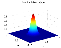
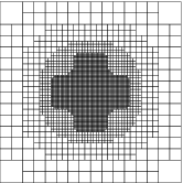
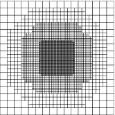
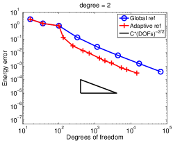
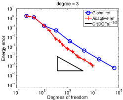
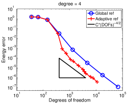
Figure 1: Some hierarchical meshes for the solution of Example 7.1; for biquadratics with $3064$ elements and $2884$ DOFs (top left), bicubics with $3028$ elements and $2809$ DOFs (top middle) and biquartics with $3400$ elements and $3160$ DOFs (top right). Notice that although all meshes have nearly the same amount of elements, the refinement is more spread for high order splines due to the sizes of the basis function supports. We plot the energy error $|u-U|_{H^{1}(\Omega)}$ vs. degrees of freedom; for biquadratics (bottom left), bicubics (bottom middle) and biquartics (bottom right).

Additionally, in Figure 2 we present the adaptive meshes obtained for different polynomial degrees, starting with an initial tensor product mesh of $4$ elements, reaching in all cases an enegy error $\approx 2.10^{-3}$. It is interesting to remark that although it is well known [Antolin et al., 2015] that the element-by-element assembly is very costly for higher degree, the use of adaptivity changes this picture. Indeed, due to the reduced number of elements for bicubics and biquartics, the time-to-solution for bicubics is $35\%$ and for biquartics is $17\%$ of the time-to-solution for biquadratics.

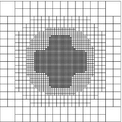
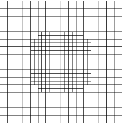
Figure 2: Comparison of adaptive meshes obtained for Example 7.1 using different polynomial degrees, obtaining in all cases that $|u-U|_{H^{1}(\Omega)}\approx 2.10^{-3}$. The mesh for biquadratics has $3064$ elements and $2884$ DOFs (left), the mesh bicubics has $688$ elements and $649$ DOFs (middle) and the mesh for biquartics has $436$ elements and $516$ DOFs (right).

Example 7.2 (Diagonal refinement in the unit square).

We take $\Omega=[0,1]\times[0,1]$ and choose $f$ and $g$ such that the exact solution $u$ of (27) is given by $u(x,y)=\tan^{-1}(25(x-y))$. In Figure 3 we plot the exact solution, some hierarchical meshes and the decay of the energy error vs. degrees of freddom for different spline degrees. As in the previous example, both tensor product meshes and hierarchical meshes reach optimal orders of convergence, but notice that in all cases, the curves corresponding to the adaptive strategy are again meaningfully by below. For example, for attaining an energy error of around $10^{-5}$ using biquadratics, the global refinement requires $67600$ DOFs whereas the adaptive strategy only needs $10186$ DOFs.

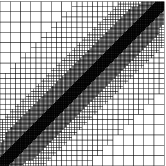
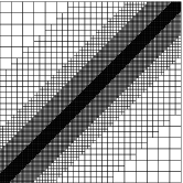
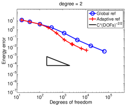
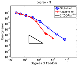
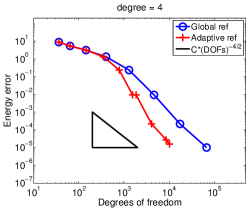
Figure 3: Some hierarchical meshes for the solution of Example 7.2; for biquadratics with $11578$ elements and $10958$ DOFs (top left), bicubics with $10792$ elements and $9865$ DOFs (top middle) and biquartics with $11338$ elements and $10186$ DOFs (top right). Notice that although all meshes have nearly the same amount of elements, the refinement is more spread for high order splines due to the sizes of the basis function supports. We plot the energy error $|u-U|_{H^{1}(\Omega)}$ vs. degrees of freedom; for biquadratics (bottom left), bicubics (bottom middle) and biquartics (bottom right).

Example 7.3 (Singular domain: an L-shaped domain).

We consider the L-shaped domain $\Omega=[-1,1]^{2}\setminus((0,1)\times(-1,0))$ and choose $f$ and $g$ such that the exact solution $u$ of (27) is given in polar coordinates by $u(\rho,\varphi)=\rho^{2/3}\sin(2\varphi/3)$. In Figure 4 we plot the exact solution, some hierarchical meshes and the decay of the energy error vs. degrees of freddom for different spline degrees. We notice that the global refinement associated to tensor product spaces does not reach the optimal order of convergence due to the singularity. On the other hand, the adaptive strategy recovers the optimal decay for the energy error given by $\mathcal{O}((\#\text{DOFs})^{\frac{p}{2}})$.

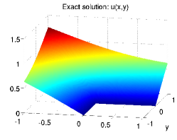
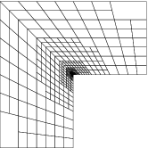
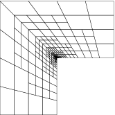
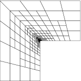
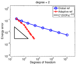
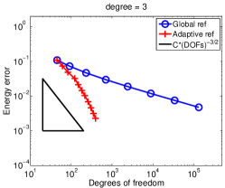
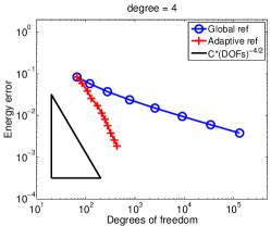
Figure 4: Some hierarchical meshes for the solution of Example 7.3 obtaining in all cases $|u-U|_{H^{1}(\Omega)}\approx 3.10^{-3}$; for biquadratics with $500$ elements and $530$ DOFs (top left), bicubics with $314$ elements and $350$ DOFs (top middle) and biquartics with $254$ elements and $322$ DOFs (top right). In addition, we plot the energy error $|u-U|_{H^{1}(\Omega)}$ vs. degrees of freedom; for biquadratics (bottom left), bicubics (bottom middle) and biquartics (bottom right).

Example 7.4 (Singular solution in the unit square).

We consider a problem whose solution is not too smooth. Specifically, we take $\Omega=[0,1]\times[0,1]$, and choose $g\equiv 0$ and $f$ such that the exact solution $u$ of (27) is given by $u(x,y)=x^{2.3}(1-x)y^{2.9}(1-y)$. Notice that in this case, $u\in H^{2}(\Omega)\setminus H^{3}(\Omega)$ and there are singularities along the sides $x=0$ and $y=0$, being a bit stronger the singularity along $x=0$; see Figure 5. Some hierarchical meshes and the error decay in terms of degrees of freddom for different polynomial degrees are presented in Figure 6. We notice that both global refinement and the adaptive refinement reach the optimal order of convergence when using biquadratics (bottom left), but only the adaptive refinement converges with optimal rates when using bicubics (bottom middle) and biquartics (bottom right), due to the singularity of the solution.

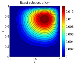
Figure 5: The exact solution $u(x,y)=x^{2.3}(1-x)y^{2.9}(1-y)$ (left) corresponding to Example 7.4 and its derivatives $u_{xx}$ (middle) and $u_{yy}$ (right).

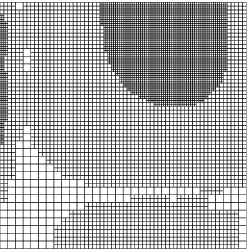
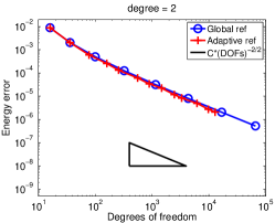
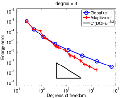
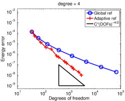
Figure 6: Comparison of adaptive meshes for the solution of Example 7.4 for different polynomial degrees, obtaining in all cases, $|u-U|_{H^{1}(\Omega)}\approx 5.10^{-6}$. The mesh for biquadratics has $6139$ elements and $6213$ DOFs (top left), the mesh for bicubics has $280$ elements and $379$ DOFs (top middle) and the mesh for biquartics has $67$ elements and $127$ DOFs (top right). On the other hand, we plot the energy error $|u-U|_{H^{1}(\Omega)}$ vs. degrees of freedom for different polynomials degrees.

Example 7.5 (A physical domain: a quarter of ring).

In this case, we consider the domain $\Omega$ given in polar coordinates by $\Omega=\{(\rho,\varphi)\mid 1\leq\rho\leq 2\quad\wedge\quad 0\leq\varphi\leq\frac{\pi}{2}\}$ and we choose the problem data $f$ and $g$ in (27) such that the exact solution $u$ is given by $u(x,y)=e^{-100((x-\frac{1}{2})^{2}+(y-\frac{1}{2})^{2})}$. Despite optimal rates of convergence are reached using both tensor product meshes and hierarchical meshes (see Figure 7), we emphasize that in this case the adaptive strategy is still convenient. As an example, we notice that to get an energy error of $2.10^{-8}$ using bicubics, the adaptive strategy requieres less than the $3\%$ of the degrees of freedom utilised by the global refinement, because the former procedure requires $1900$ DOFs whereas the latter needs $67081$ DOFs.

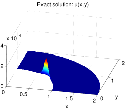
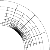
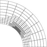
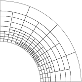
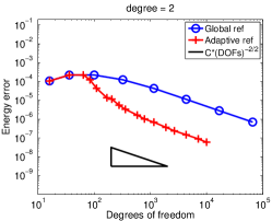
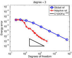
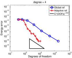
Figure 7: Some hierarchical meshes for the solution of Example 7.5 obtaining $|u-U|_{H^{1}(\Omega)}\approx 1.10^{-6}$ in all cases; for biquadratics with $802$ elements and $788$ DOFs (top left), bicubics with $316$ elements and $349$ DOFs (top middle) and biquartics with $160$ elements and $216$ DOFs (top right). We plot the energy error $|u-U|_{H^{1}(\Omega)}$ vs. degrees of freedom; for biquadratics (bottom left), bicubics (bottom middle) and biquartics (bottom right).

Example 7.6 (A $3d$-domain: the unit cube).

We consider the cube $\Omega=[0,1]^{3}$ and choose $f$ and $g$ such that the exact solution $u$ of (27) is given by $u(x,y,z)=e^{-100((x-\frac{1}{2})^{2}+(y-\frac{1}{2})^{2}+(z-\frac{1}{2})^{2})}$. Since the solution is smooth enough, both strategies reach optimal orders of convergence, as showed in Figure 8. However, we notice that in all cases, the curves corresponding to the adaptive strategy are meaningfully by below, which in practice is equivalent to achieve a given accuracy with considerably fewer degrees of freddom.

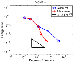
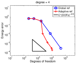
Figure 8: Energy error decay in terms of degrees of freedom for the solution of the Example 7.6; using biquadratics (left), bicubics (middle) and biquartics (right).

On the efficiency of the error estimators

Finally, we analyse the behaviour of the efficiency index $\frac{\left(\sum_{\beta\in\mathcal{H}}\mathcal{E}_{\beta}^{2}\right)^{\frac{1}{2}}}{\|\nabla(u-U)\|_{L^{2}(\Omega)}}$. In Figure 9, we plot this index at each iteration step for all the examples previously presented. We see that the energy error $\|\nabla(u-U)\|_{L^{2}(\Omega)}$ and the global a posteriori error estimator $\left(\sum_{\beta\in\mathcal{H}}\mathcal{E}_{\beta}^{2}\right)^{\frac{1}{2}}$ are equivalent quantities, that is, there exists constants $c_{1}$ and $c_{2}$ such that

$$0<c_{1}\leq\frac{\left(\sum_{\beta\in\mathcal{H}}\mathcal{E}_{\beta}^{2}\right)^{\frac{1}{2}}}{\|\nabla(u-U)\|_{L^{2}(\Omega)}}\leq c_{2},$$

at each iteration step. Thus, we conclude that our estimators are not only reliable but also experimentally efficient.

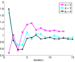
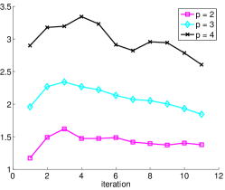
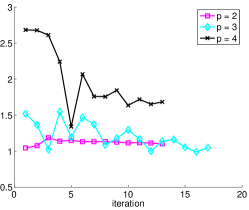
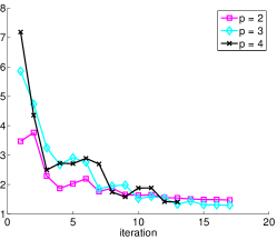
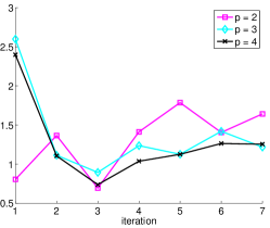
Figure 9: Efficiency indices $\frac{\frac{1}{10}\left(\sum_{\beta\in\mathcal{H}}\mathcal{E}_{\beta}^{2}\right)^{\frac{1}{2}}}{\|\nabla(u-U)\|_{L^{2}(\Omega)}}$; for Example 7.1 (top left), Example 7.2 (top middle), Example 7.3 (top right), Example 7.4 (bottom left), Example 7.5 (bottom middle), Example 7.6 (bottom right).

References

- [Antolin et al., 2015] Antolin, P., Buffa, A., Calabrò, F., Martinelli, M., and Sangalli, G. (2015). Efficient matrix computation for tensor-product isogeometric analysis: the use of sum factorization Comput. Methods Appl. Mech. Engrg., 285, 817–828.
- [Babuška and Rheinboldt, 1978] Babuška, I. and Rheinboldt, W. C. (1978). Error estimates for adaptive finite element computations. SIAM J. Numer. Anal., 15(4):736–754.
- [Buffa and Garau, 2016] Buffa, A. and Garau, E. M. (2016). Refinable spaces and local approximation estimates for hierarchical splines. IMA J. Numer. Anal. First published online: July 27, 2016.
- [Buffa and Giannelli, 2016] Buffa, A. and Giannelli, C. (2016). Adaptive isogeometric methods with hierarchical splines: Error estimator and convergence. Mathematical Models and Methods in Applied Sciences, 26(01):1–25.
- [Cascon et al., 2008] Cascon, J. M., Kreuzer, C., Nochetto, R. H., and Siebert, K. G. (2008). Quasi-optimal convergence rate for an adaptive finite element method. SIAM J. Numer. Anal., 46(5):2524–2550.
- [Chua and Wheeden, 2006] Chua, S.-K. and Wheeden, R. L. (2006). Estimates of best constants for weighted Poincaré inequalities on convex domains. Proc. London Math. Soc. (3), 93(1):197–226.
- [Cottrell et al., 2009] Cottrell, J. A., Hughes, T. J. R., and Bazilevs, Y. (2009). Isogeometric Analysis: toward integration of CAD and FEA. John Wiley & Sons.
- [Curry and Schoenberg, 1966] Curry, H. B. and Schoenberg, I. J. (1966). On Pólya frequency functions. IV. The fundamental spline functions and their limits. J. Analyse Math., 17:71–107.
- [de Boor, 2001] de Boor, C. (2001). A practical guide to splines, volume 27 of Applied Mathematical Sciences. Springer-Verlag, New York, revised edition.
- [Garau and Vázquez, 2016] Garau, E. M. and Vázquez, R. (2016). Algorithms for the implementation of adaptive isogeometric methods using hierarchical splines. Technical report, IMAL (CONICET-UNL).
- [Giannelli et al., 2012] Giannelli, C., Jüttler, B., and Speleers, H. (2012). THB-splines: The truncated basis for hierarchical splines. Comput. Aided Geom. Design., 29(7):485 – 498.
- [Giannelli et al., 2014] Giannelli, C., Jüttler, B., and Speleers, H. (2014). Strongly stable bases for adaptively refined multilevel spline spaces. Adv. Comput. Math., 40(2):459–490.
- [Hughes et al., 2005] Hughes, T. J. R., Cottrell, J. A., and Bazilevs, Y. (2005). Isogeometric analysis: CAD, finite elements, NURBS, exact geometry and mesh refinement. Comput. Methods Appl. Mech. Engrg., 194(39-41):4135–4195.
- [Kraft, 1997] Kraft, R. (1997). Adaptive and linearly independent multilevel -splines. In Surface fitting and multiresolution methods (Chamonix–Mont-Blanc, 1996), pages 209–218. Vanderbilt Univ. Press, Nashville, TN.
- [Morin et al., 2003] Morin, P., Nochetto, R. H., and Siebert, K. G. (2003). Local problems on stars: a posteriori error estimators, convergence, and performance. Math. Comp., 72(243):1067–1097 (electronic).
- [Schumaker, 2007] Schumaker, L. L. (2007). Spline functions: basic theory. Cambridge Mathematical Library. Cambridge University Press, Cambridge, third edition.
- [Veeser and Verfürth, 2009] Veeser, A. and Verfürth, R. (2009). Explicit upper bounds for dual norms of residuals. SIAM J. Numer. Anal., 47(3):2387–2405.
- [Vuong et al., 2011] Vuong, A.-V., Giannelli, C., Jüttler, B., and Simeon, B. (2011). A hierarchical approach to adaptive local refinement in isogeometric analysis. Comput. Methods Appl. Mech. Engrg., 200(49-52):3554–3567.