Spin fluctuations and high-temperature superconductivity in cuprates

Abstract

To describe the cuprate superconductors, models of strongly correlated electronic systems, such as the Hubbard or $t$-$J$ models, are commonly employed. To study these models, projected (Hubbard) operators have to be used. Due to the unconventional commutation relations for the Hubbard operators, a specific kinematical interaction of electrons with spin and charge fluctuations emerges. The interaction is induced by the intraband hopping with a coupling parameter of the order of the kinetic energy of electrons $\,W$ which is much larger than the antiferromagnetic exchange interaction $J$ induced by the interband hopping. This review presents a consistent microscopic theory of spin excitations and superconductivity for cuprates where these interactions are taken into account within the Hubbard operator technique. The low-energy spin excitations are considered for the $t$–$J$ model, while the electronic properties are studied using the two-subband extended Hubbard model where the intersite Coulomb repulsion $V$ and electron-phonon interaction are taken into account.

I Introduction

Discovery of high-temperature superconductivity (HTSC) in cuprates by Bednorz and Müller Bednorz86 caused an unprecedented scientific activity in study of this extraordinary phenomenon (see, e.g., Refs. Schrieffer07 ; Plakida10 ). In recent years intensive experimental investigations have presented detailed information concerning unconventional physical properties of cuprates. However, theoretical studies of various microscopical models have not yet brought about a commonly accepted theory of superconductivity in cuprates. Two most frequently discussed mechanisms of HTSC are the conventional electron-phonon pairing (see, e.g., Refs. Kulic04 ; Maksimov10 ) and the spin-fluctuation mediated pairing Scalapino95 ; Scalapino12 in the framework of phenomenological spin-fermion models (see, e.g., Refs. Monthoux94b ; Moriya00 ; Chubukov04 ; Abanov08 ). A weak intensity of spin fluctuations at optimal doping found in the magnetic inelastic neutron scattering experiments Bourges98 is the main argument against the spin-fluctuation pairing mechanism. However, recent magnetic resonant inelastic x-ray scattering (RIXS) experiments have revealed that paramagnon antiferromagnetic (AF) excitations persist with a similar dispersion and comparable intensity in a large family of cuprate superconductors, even in the overdoped region (see, e.g., Refs. LeTacon11 ; LeTacon13 ; Dean13 ; Dean14 ; Minola15 ). These experiments prove that spin fluctuations have sufficient strength to mediate HTSC in cuprates and to explain various physical properties of cuprate materials such as, the “kink” phenomenon observed in the electronic spectrum by the angle-resolved photoemission spectroscopy Kordyuk10 , the optical and dc conductivity Vladimirov12 , etc. Therefore, we can assume that the spin-fluctuation mediated pairing plays the major role while the electron-phonon pairing is less important. This assumption is supported by observation of the weak isotope effect in optimally doped samples (see reviews  Zhao01 ; Khasanov04 ; Muller07 ).

The main problem in a theoretical study of the cuprate superconductors is that strong electron correlations there precludes from application of the conventional Fermi-liquid approach in description of their electronic structure Fulde95 . They are Mott-Hubbard (more accurately, charge-transfer) insulators where the conduction band splits into two Hubbard subbands where the projected (Hubbard) electronic operators should be used. Recently we have developed a microscopic theory of spin excitations and superconductivity for cuprates within the Hubbard operator (HO) technique  Plakida10 ; Vladimirov09 ; Vladimirov11 ; Plakida06 ; Plakida07 ; Plakida13 ; Plakida14 . We demonstrate an important role of the kinematical interaction for the HOs induced by the non-Fermy commutation relations for electronic operators, both for studying the spin excitations and electron spectrum. In this review we present the results of these investigations.

First, in Sec. II, we explain how the kinematical interaction appears in the Hubbard model in the limit of strong electron correlations. Then in Sec. III we formulate a theory of spin excitations within the relaxation-function approach for calculation of the dynamical spin susceptibility (DSS) in the normal and superconducting states  Vladimirov09 ; Vladimirov11 . The spin dynamics at arbitrary frequencies and wave vectors is studied for various temperatures and hole doping. In the superconducting state, the DSS reveals the magnetic resonance mode at the AF wave vector ${\bf Q}=\pi(1,1)$ at low doping. We show that it can be observed even above superconducting $T_{c}$ due to its weak damping. This is explained by an involvement of spin excitations in the decay process besides the particle-hole continuum usually considered in the random-phase-type approximation where the resonance mode can appear only below $T_{c}$.

In the second part of the paper, in Secs. IV and V, a theory of the electronic spectrum and superconductivity is presented within the Mori-type projection technique for the single-particle electronic Green functions (GFs) Plakida07 ; Plakida13 ; Plakida14 . We consider the extended Hubbard model where the intersite Coulomb repulsion and the electron-phonon interaction are taken into account. An exact Dyson equation for the normal and anomalous (pair) GFs is derived which is solved in the self-consistent Born approximation (SCBA) for the self-energy. We found the $d$-wave pairing with high-$T_{c}$ mediated by the kinematical spin-fluctuation interaction which can be suppressed only for a large intersite Coulomb repulsion $\,V>W$. Isotope effect on $T_{c}$ induced by electron-phonon interaction is weak at optimal doping and increases at low doping. We emphasize that the kinematical interaction is absent in the spin-fermion models and is lost in the slave-boson (-fermion) models treated in the mean-field approximation (MFA). In conclusion we summarize our results.

II Kinematical interaction in the Hubbard model

We consider the extended Hubbard model Hubbard63 on a square lattice

$$H = \sum_{i\neq j,\sigma}\,t_{ij}\,a_{i\sigma}^{{\dagger}}a_{j\sigma}-\mu\,\sum_{i}N_{i}$$ (1)

$$+ (U/2)\,\sum_{i}N_{i\sigma}N_{i\bar{\sigma}}+(1/2)\,\sum_{i\neq j}V_{ij}\,N_{i}N_{j},$$

where $t_{i,j}$ is the single-electron hopping parameter, $a^{{\dagger}}_{i\sigma}$ and $a_{i\sigma}$ are the Fermi creation and annihilation operators for electrons with spin $\sigma/2\;(\sigma=\pm 1),\,\bar{\sigma}=-\sigma)$ on the lattice site $i$, $U$ is the on-site Coulomb interaction (CI) and the $V_{ij}$ is the intersite CI. $\,N_{i}=\sum_{\sigma}N_{i\sigma},\,N_{i\sigma}=a^{{\dagger}}_{i\sigma}a_{i\sigma}$ is the number operator and $\mu$ is the chemical potential.

In the strong correlation limit, $U\gg|t_{i,j}|$, the Fermi operators $a^{\dagger}_{i\sigma},\,a_{i\sigma}$ in (1) fail to describe single-particle electron excitations in the system and the HOs Hubbard65 , referring to the singly occupied and doubly occupied subbands, should be used: $a^{\dagger}_{i\sigma}=a^{\dagger}_{i\sigma}(1-N_{i\bar{\sigma}})+a^{\dagger}_{i\sigma}N_{i\bar{\sigma}}\equiv X_{i}^{\sigma 0}+\sigma\,X_{i}^{2\bar{\sigma}}$. In terms of the HOs the model (1) reads

$$H = \varepsilon_{1}\sum_{i,\sigma}X_{i}^{\sigma\sigma}+\varepsilon_{2}\sum_{i}X_{i}^{22}+\frac{1}{2}\sum_{i\neq j}\,V_{ij}N_{i}N_{j}$$ (2)

$$+ \sum_{i\neq j,\sigma}\,t_{ij}\,\bigl{\{}X_{i}^{\sigma 0}X_{j}^{0\sigma}+X_{i}^{2\sigma}X_{j}^{\sigma 2}$$

$$+ \sigma\,(X_{i}^{2\bar{\sigma}}X_{j}^{0\sigma}+{\rm H.c.})\bigr{\}},$$

where $\varepsilon_{1}=-\mu$ is the single-particle energy and $\varepsilon_{2}=U-2\mu$ is the two-particle energy. The matrix HOs $X_{i}^{\alpha\beta}=|i\alpha\rangle\langle i\beta|$ describes transition from the state $|i,\beta\rangle$ to the state $|i,\alpha\rangle$ on a lattice site $i$ taking into account four possible states for holes: an empty state $(\alpha,\beta=0)$, a singly occupied hole state $(\alpha,\beta=\sigma)$, and a doubly occupied hole state $(\alpha,\beta=2)$. The number operator and the spin operators in terms of the HOs are defined as

$$N_{i} = \sum_{\sigma}X_{i}^{\sigma\sigma}+2X_{i}^{22},$$ (3)

$$S_{i}^{\sigma} = X_{i}^{\sigma\bar{\sigma}},\quad S_{i}^{z}=(\sigma/2)\,[X_{i}^{\sigma\sigma}-X_{i}^{\bar{\sigma}\bar{\sigma}}].$$ (4)

To compare our results with cuprates, we consider the hole-doped case where the chemical potential $\mu$ is determined by the equation for the average hole occupation number

$$n=1+\delta=\langle\,N_{i}\rangle.$$ (5)

Here $\langle\ldots\rangle$ denotes the statistical average with the Hamiltonian (2).

From the multiplication rule for the HOs, $\,X_{i}^{\alpha\beta}X_{i}^{\gamma\delta}=\delta_{\beta\gamma}X_{i}^{\alpha\delta}$, it follows their commutation relations

$$\left[X_{i}^{\alpha\beta},X_{j}^{\gamma\delta}\right]_{\pm}=\delta_{ij}\left(\delta_{\beta\gamma}X_{i}^{\alpha\delta}\pm\delta_{\delta\alpha}X_{i}^{\gamma\beta}\right)\,,$$ (6)

with the upper sign for the Fermi-type operators (such as $X_{i}^{0\sigma}$) and the lower sign for the Bose-type operators (such as the number or spin operators). The HOs obey the completeness relation

$$X_{i}^{00}+\sum_{\sigma}X_{i}^{\sigma\sigma}+X_{i}^{22}=1,$$ (7)

which rigorously preserves the local constraint that only one quantum state $\alpha$ can be occupied on any lattice site $i$.

The unconventional commutation relations (6) for HOs result in the kinematical interaction. The term was introduced by Dyson in a general theory of spin-wave interactions  Dyson56 . It was pointed out that the spin-wave creation $\,b_{i}^{{\dagger}}=S_{i}^{-}$ and annihilation $\,b_{i}=S_{i}^{+}\,$ operators obey the commutation relations

$$b_{i}b_{j}^{{\dagger}}-b_{j}^{{\dagger}}b_{i}=\delta_{i,j}\,(1-2\,b_{i}^{{\dagger}}b_{i}),$$ (8)

which show that they are Bose operators on different lattice sites and Fermi operators on the same lattice site. The last term $\,b_{i}^{{\dagger}}b_{i}\,$ in Eq. (8) just brings about the kinematical interaction which may be small for low density of spin excitations, $\,b_{i}^{{\dagger}}b_{i}\ll 1\,$.

Similar commutation relations can be written for the electron creation $X_{i}^{\sigma 0}\,$ and annihilation $X_{j}^{0\sigma}\,$ operators,

$$X_{i}^{0\sigma}X_{j}^{\sigma 0}+X_{j}^{\sigma 0}X_{i}^{0\sigma}=\delta_{i,j}(1-X_{i}^{\bar{\sigma}\bar{\sigma}}-X_{i}^{22})$$

$$=\delta_{ij}(1-N_{i\sigma}/2+\sigma S_{i}^{z}),$$ (9)

where the relation (7) was used. Therefore, the HOs for electrons in the singly occupied subband can be considered as Fermi operators on different lattice sites but on the same lattice site electron scattering on charge $N_{i\sigma}$ and spin $S_{i}^{\alpha}$ fluctuations occurs which determines the kinematical interaction. This results in dressing of the electron hopping by spin and charge fluctuations with the coupling constant of the order of the hopping parameter $\,t$.

III Spin excitation spectrum

To study low-energy excitations such as spin excitations in the limit of strong correlations, $U\gg t$, we can consider only one subband, e.g., the singly occupied subband for electrons taking into account virtual hopping to the second subband by the exchange interaction $J_{ij}=4\,t_{ij}^{2}/U$. This results in the $t$-$J$ model which in terms of the HOs reads

$$H = -\sum_{i\neq j,\sigma}t_{ij}X_{i}^{\sigma 0}X_{j}^{0\sigma}-\mu\sum_{i\sigma}X_{i}^{\sigma\sigma}$$ (10)

$$+ \frac{1}{4}\sum_{i\neq j,\sigma}J_{ij}\left(X_{i}^{\sigma\bar{\sigma}}X_{j}^{\bar{\sigma}\sigma}-X_{i}^{\sigma\sigma}X_{j}^{\bar{\sigma}\bar{\sigma}}\right).$$

In the $t$-$J$ model the doubly-occupied states are neglected and therefore the number operator (3) and the completeness relation (7) take the forms: $\,n_{i}=\sum_{\sigma}\,X_{i}^{\sigma\sigma}$ and $X_{i}^{00}+\sum_{\sigma}X_{i}^{\sigma\sigma}=1$, respectively. The chemical potential $\mu$ is determined from the equation for the average electron density

$$n=\sum_{\sigma}\langle X_{i}^{\sigma\sigma}\rangle=1-\delta,$$ (11)

where $\delta=\langle X_{i}^{00}\rangle$ is the hole concentration and $\langle\ldots\rangle$ denotes the statistical average with the Hamiltonian (10).

Various approaches have been used to study the spin dynamics within the $t$ -$J$ model (10) (for a review see, e.g., Refs. Izyumov97 and  Plakida06 ). In particular, in the slave boson or fermion methods, a local constraint prohibiting a double occupancy of any quantum state is difficult to treat rigorously. An application of a special diagram technique for HOs in the $t$–$J$ model results in a complicated analytical expression for the DSS Izyumov90 . Studies of finite clusters by numerical methods were important in elucidating static and dynamic spin interactions, though they have limited energy and momentum resolutions (see, e.g., Refs. Dagotto94 ; Jaklic00 ; Eder95 ).

To overcome this complexity, we apply the projection Mori-type technique elaborated for the two-time thermodynamic GFs Zubarev60 ; Plakida73 ; Tserkovnikov81 ; Plakida11 . In this method an exact representation for the self-energy (or polarization operator) can be derived which, when evaluated in the mode-coupling approximation (MCA), yields physically reasonable results even for strongly interacting systems.

We use the spin-rotation-invariant relaxation-function theory for the DSS to calculate the static properties in the generalized mean-field approximation (GMFA) similarly to Ref. Winterfeldt98 and the dynamic spin-fluctuation spectra using the MCA for the force-force correlation functions. Thereby, we capture both the local and itinerant character of charge carriers in a consistent way. In calculating the static properties, in particular the static susceptibility and spin-excitation spectrum, we pay particular attention to a proper description of AF short-range order (SRO) and its implications on the spin dynamics. For the undoped case described by the Heisenberg model our results are similar to those in Refs. Winterfeldt97 and  Winterfeldt99 . For a finite doping our theory yields a reasonable agreement with available exact diagonalization (ED) data and neutron scattering experiments.

A similar approach based on the Mori projection technique for the single-particle electron GF and spin GF has been used in Refs. Sega03 ; Prelovsek04 ; Sherman03 ; Sherman04 ; Sherman06 . The magnetic resonance mode observed in the superconducting state was studied within the memory-function approach in Refs. Sherman03a ; Sega03 ; Sega06 ; Prelovsek06 .

First we present the results for the DSS in the normal state obtained in Ref. Vladimirov09 and then we consider the theory of the magnetic resonance mode in the superconducting state developed in Ref. Vladimirov11 .

III.1 Relaxation-function theory

In Ref. Vladimirov05 , applying the Mori-type projection technique Mori65 , elaborated for the relaxation function, we have derived an exact representation for the DSS $\,\chi({\bf q},\omega)\,$ related to the retarded commutator GF Zubarev60 ,

$$\chi({\bf q},\omega)=-\langle\!\langle{S}_{\bf q}^{+}|{S}_{-\bf q}^{-}\rangle\!\rangle_{\omega}=\frac{m({\bf q})}{\omega_{\bf q}^{2}+\omega\,\Sigma({\bf q},\omega)-\omega^{2}},$$ (12)

where $m({\bf q})=\langle[i\dot{S}^{+}_{\bf q},S_{-\bf q}^{-}]\rangle=\langle[\,[{S}^{+}_{\bf q},H],\,S_{-\bf q}^{-}]\rangle$, and $\omega_{\bf q}$ is the spin-excitation spectrum in the GMFA. The self-energy is given by the many-particle Kubo-Mori relaxation function

$$\Sigma({\bf q},\omega)=[1/m({\bf q})]\,(\!(-\ddot{S}_{\bf q}^{+}\,|-\ddot{S}_{-\bf q}^{-})\!)_{\omega}^{(\rm pp)}\,,$$ (13)

where $-\ddot{S}_{\bf q}^{\pm}=[\,[{S}_{\bf q}^{\pm},H],\,H]$ (for details see Ref. Vladimirov05 ). The Kubo-Mori relaxation function and the scalar product are defined as (see, e.g., Ref. Tserkovnikov81 )

$$((A|B))_{\omega}=-i\int_{0}^{\infty}dte^{i\omega t}(A(t),B),$$ (14)

and

$$(A(t),B)=\int_{0}^{\beta}d\lambda\langle A(t-i\lambda)B\rangle,\quad\beta=1/k_{\rm B}T,$$ (15)

respectively. The “proper part” (pp) of the relaxation function (13) does not contain parts connected by a single zero-order relaxation function which corresponds to the projected time evolution in the original Mori projection technique Mori65 . The spin-excitation spectrum is given by the spectral function defined by the imaginary part of the DSS (12),

$$\chi^{\prime\prime}({\bf q},\omega)=\frac{-\omega\,\Sigma{{}^{\prime\prime}}({\bf q},\omega)\;m({\bf q})}{[\omega^{2}-\omega_{\bf q}^{2}-\omega\,\Sigma{{}^{\prime}}({\bf q},\omega)]^{2}+[\omega\,\Sigma{{}^{\prime\prime}}({\bf q},\omega)]^{2}}\,,$$ (16)

where $\,\Sigma({\bf q},\omega+i0^{+})=\Sigma{{}^{\prime}}({\bf q},\omega)+i\Sigma{{}^{\prime\prime}}({\bf q},\omega)$ and $\,\Sigma{{}^{\prime}}({\bf q},\omega)=-\Sigma{{}^{\prime}}({\bf q},-\omega)$ is the real and $\Sigma{{}^{\prime\prime}}({\bf q},\omega)=\Sigma{{}^{\prime\prime}}({\bf q},-\omega)<0$ is the imaginary parts of the self-energy.

Static properties. The general representation of the DSS (12) determines the static susceptibility $\,\chi_{\bf q}=\chi({\bf q},0)\,$ by the equation

$$\chi_{\bf q}=({S}_{\bf q}^{+},S_{-{\bf q}}^{-})=m({\bf q})/\omega_{\bf q}^{2}\,.$$ (17)

To calculate the spin-excitation spectrum $\omega_{\bf q}$ we use the equality for $m({\bf q})=\langle[\,[{S}^{+}_{\bf q},H],\,S_{-\bf q}^{-}]\rangle$:

$$m({\bf q})=(-\ddot{S}_{\bf q}^{+},S_{-{\bf q}}^{-})=\omega_{\bf q}^{2}\,({S}_{\bf q}^{+},S_{-{\bf q}}^{-}),$$ (18)

where the correlation function $(-\ddot{S}_{\bf q}^{+},S_{-{\bf q}}^{-})$ is evaluated in the GMFA by a decoupling procedure in the site representation as described in Ref. Vladimirov09 . This procedure is equivalent to the MCA for the equal-time correlation functions. This results in the spin-excitation spectrum

$$\omega_{\bf q}^{2} = 8t^{2}\lambda_{1}(1-\gamma_{\bf q})(1-n-F_{2,0}-2F_{1,1})$$ (19)

$$+ 4J^{2}(1-\gamma_{\bf q})\big{[}\,\lambda_{2}\frac{n}{2}-\alpha_{1}C_{1,0}(4\gamma_{\bf q}+1)$$

$$+ \alpha_{2}(2C_{1,1}+C_{2,0})\,\big{]},$$

where $t$ and $J$ are the hopping parameter and the exchange interaction for the nearest neighbors, respectively, and $\gamma_{\bf q}=(1/2)\,(\cos q_{x}+\cos q_{y})$ (we take the lattice spacing $a$ to be unity). The static electron and spin correlation functions are defined as

$$F_{n,m}\equiv F_{\bf R} = \langle X_{\bf 0}^{\sigma 0}\,X_{\bf R}^{0\sigma}\rangle=\frac{1}{N}\sum_{{\bf q}}\,F_{\bf q}{\rm e}^{i{\bf qR}},$$ (20)

$$C_{n,m}\equiv C_{\bf R} = \langle S^{-}_{\bf 0}\,S^{+}_{\bf R}\rangle=\frac{1}{N}\sum_{{\bf q}}\,C_{\bf q}{\rm e}^{i{\bf qR}},$$ (21)

where ${\bf R}=n{\bf a}_{x}+m{\bf a}_{y}\,$ and $C_{\bf q}=\langle S^{+}_{\bf q}S^{-}_{-\bf q}\rangle$. The direct calculation of $m({\bf q})=\langle[\,[{S}^{+}_{\bf q},H],\,S_{-\bf q}^{-}]\rangle$ yields

$$m({\bf q})=-8\,(1-\gamma_{\bf q})\,\left[t\,F_{1,0}+J\,C_{1,0}\right].$$ (22)

The AF correlation length $\xi$ may be calculated by expanding the static susceptibility in the neighborhood of the AF wave vector ${\bf Q}=\pi(1,1)$, $\chi_{\bf Q+\bf k}=\chi_{\bf Q}/(1+\xi^{2}\,k^{2})$ Shimahara91 ; Winterfeldt97 . We get

$$\xi^{2}=\frac{8J^{2}\alpha_{1}|C_{1,0}|}{\omega_{\bf Q}^{2}}.$$ (23)

The critical behavior of the model (10) is reflected by the divergence of $\chi_{\bf Q}$ and $\xi$ as $T\rightarrow 0$, i.e., by $\omega_{\bf Q}(T=0)=0$. In the phase with AF long-range order (LRO) which, in two dimensions, may occur at $T=0$ only, the correlation function $C_{\bf R}$ (21) is written as Shimahara91 ; Winterfeldt97

$$C_{\bf R}=\frac{1}{N}\sum_{{\bf q}\neq{\bf Q}}\,C_{\bf q}{\rm e}^{i{\bf qR}}+C\,{\rm e}^{i{\bf QR}}.$$ (24)

The condensation part $C$ determines the staggered magnetization $\,|m|=|\langle S_{i}^{z}\rangle|\,$ which in the spin-rotation-invariant form is given by

$$m^{2}=\frac{3}{2N}\sum_{\bf R}\,C_{\bf R}{\rm e}^{-i{\bf QR}}=\frac{3}{2}\,C.$$ (25)

The GMFA spectrum (19) is calculated self-consistently by using this spectrum for the static correlation function (21),

$$C_{\bf q}=\frac{m({\bf q})}{2\,\omega_{\bf q}}\,\coth\frac{\beta\,\omega_{\bf q}}{2}\,.$$ (26)

The decoupling parameters $\alpha_{1},\alpha_{2}$ and $\lambda_{1},\lambda_{2}$ in Eq. (19) take into account the vertex renormalization for the spin-spin and electron-spin interaction, respectively, as explained in Ref. Vladimirov09 . In particular, the parameters $\alpha_{1},\alpha_{2}$ are evaluated from the results for the Heisenberg model at $\delta=0$ and are kept fixed for $\delta\neq 0$. The parameters $\lambda_{1},\lambda_{2}$ are calculated from the sum rule $C_{0,0}=\langle S^{+}_{0}S^{-}_{0}\rangle=(1/2)(1-\delta)$ with a fixed ratio $\lambda_{1}/\lambda_{2}=0.378$. In the superconducting state, the electron correlation function $\,F_{\bf R}\,$ is calculated by the spectral function for electrons in the superconducting state. The variation of the parameters $\lambda_{1},\lambda_{2}$ below the superconducting transition is negligibly small and practically has no influence on the spectrum $\omega_{\bf q}$.

Thus, the static susceptibility (17) is explicitly determined by Eqs. (19) and (22).

Self-energy. The self-energy (13) can be written in terms of the corresponding time-dependent correlation functions as

$$\Sigma({\bf q},\omega)=\frac{1}{2\pi m({\bf q})}\int_{-\infty}^{\infty}d\omega^{\prime}\frac{e^{\beta\omega^{\prime}}-1}{\omega^{\prime}(\omega-\omega^{\prime})}$$

$$\,\int_{-\infty}^{\infty}dte^{i\omega^{\prime}t}\langle\,\ddot{S}^{-}_{-\bf q}\;\ddot{S}^{+}_{\bf q}(t)\rangle^{\rm pp},$$ (27)

where $-\ddot{S}_{i}^{+}=[[{S}_{i}^{+},\,(H_{t}+H_{J})]\,,\,(H_{t}+H_{J})]\equiv\sum_{\alpha}F_{i}^{\alpha}$, and $H_{t}$ and $H_{J}$ are the hopping and the exchange parts of the Hamiltonia (10) and $\alpha=tt,\,tJ,\,Jt,\,JJ$. As shown in Ref. Vladimirov09 , the largest contribution at a finite hole doping $\delta>0.05$ in (27) comes from the spin-electron scattering, the $F_{i}^{tt}$ forces. In the undoped case, $\delta=0$, for the Heisenberg model we should take into account the $F_{i}^{JJ}$ forces.

Using MCA for the corresponding time-depending correlation functions of the forces, the spin-electron scattering contribution to the imaginary part of the self-energy $\Sigma^{\prime\prime}_{t}({\bf q},\omega)$ in the superconducting state can be written as

$$\Sigma^{\prime\prime}_{t}({\bf q},\omega)=-\frac{\pi(2t)^{4}(e^{\beta\omega}-1)}{m({\bf q})\,\omega}\int\!\!\int_{-\infty}^{\infty}d\omega_{1}d\omega_{2}$$ (28)

$$\times\frac{1}{N^{2}}\sum_{{\bf q_{1},q_{2}}}[1-n(\omega_{1})]\,n(\omega+\omega_{1}-\omega_{2})\,N(\omega_{2})B_{\bf q_{2}}(\omega_{2})$$

$$\times\big{[}({\Lambda}^{2}_{\bf q_{1},q_{2},q_{3}}+{\Lambda}^{2}_{\bf q_{3},q_{2},q_{1}})\,A^{N}_{\bf q_{1}}(\omega_{1})\,A^{N}_{\bf q_{3}}(\omega+\omega_{1}-\omega_{2})$$

$$-2{\Lambda}_{\bf q_{1},q_{2},q_{3}}{\Lambda}_{\bf q_{3},q_{2},q_{1}}\,A^{S}_{{\bf q_{1}}\sigma}(\omega_{1})\,A^{S}_{{\bf q_{3}}\sigma}(\omega+\omega_{1}-\omega_{2})\big{]},$$

where ${\bf q}={\bf q}_{1}+{\bf q}_{2}+{\bf q}_{3}\,$. The Fermi and Bose functions are denoted by $n(\omega)=(e^{\beta\omega}+1)^{-1}$ and $N(\omega)=(e^{\beta\omega}-1)^{-1}$. The vertex function $\Lambda_{\bf q_{1},q_{2},q_{3}}$ is defined by the equation

$$\Lambda_{{\bf q}_{1}{\bf q}_{2}{\bf q}_{3}}=4(\gamma_{{\bf q}_{3}+{\bf q}_{2}}-\gamma_{{\bf q}_{1}})\,\gamma_{q_{3}}+\gamma_{{\bf q}_{2}}-\gamma_{{\bf q}_{1}+{\bf q}_{3}},$$ (29)

where the terms linear in $\gamma_{{\bf q}}$ reflect the exclusion of terms in $F_{i}^{tt}$ with coinciding sites. Here we introduced the spectral functions:

$$A^{N}_{\bf q}(\omega) = -(1/\pi){\rm Im}\langle\langle X^{0\sigma}_{\bf q}|X^{\sigma 0}_{\bf q}\rangle\rangle_{\omega},$$ (30)

$$A^{S}_{{\bf q}\sigma}(\omega) = -(1/\pi){\rm Im}\langle\langle X^{0\sigma}_{\bf q}|X^{0\bar{\sigma}}_{-\bf q}\rangle\rangle_{\omega},$$ (31)

$$B_{\bf q}(\omega) = (1/\pi)\,\chi^{\prime\prime}({\bf q},\omega),$$ (32)

where $A^{N,S}_{\bf q}(\omega)$ are determined by the retarded anticommutator GFs for electrons Zubarev60 . In the normal state, the contribution proportional to the anomalous GF $\,\langle\langle X^{0\sigma}_{\bf q}|X^{0\bar{\sigma}}_{-\bf q}\rangle\rangle_{\omega}\,$ disappears.

The self-energy $\Sigma^{\prime\prime}_{J}({\bf q},\omega)$ for the Heisenberg model in the undoped case reads

$$\Sigma^{\prime\prime}_{J}({\bf q},\omega)=\frac{\pi\,(2\,J)^{4}\,(e^{\beta\omega}-1)}{2\,m({\bf q})\,\omega}\frac{1}{N^{2}}\sum_{{\bf q}_{1},{\bf q}_{2}}\int\!\!\int_{-\infty}^{\infty}d\omega_{1}d\omega_{2}$$

$$\times\{\Gamma^{2}_{{\bf q}_{1}{\bf q}_{2}{\bf q}_{3}}+\Gamma_{{\bf q}_{1}{\bf q}_{2}{\bf q}_{3}}\Gamma_{{\bf q}_{2}{\bf q}_{1}{\bf q}_{3}}\}N(\omega_{1})N(\omega_{2})$$ (33)

$$\times N(\omega-\omega_{1}-\omega_{2})B_{{\bf q}_{1}}(\omega_{1})B_{{\bf q}_{2}}(\omega_{2})B_{{\bf q}_{3}}(\omega-\omega_{1}-\omega_{2}),$$

where ${\bf q}={\bf q}_{1}+{\bf q}_{2}+{\bf q}_{3}\,$. The vertex for the spin-spin scattering reads

$$\Gamma_{{\bf q}_{1}{\bf q}_{2}{\bf q}_{3}}=4(\gamma_{{\bf q}_{3}+{\bf q}_{1}}-\gamma_{{\bf q}_{2}})(\gamma_{{\bf q}_{3}}-\gamma_{{\bf q}_{1}})$$

$$-\gamma_{{\bf q}_{1}}+\gamma_{{\bf q}_{3}}+\gamma_{{\bf q}_{2}+{\bf q}_{3}}-\gamma_{{\bf q}_{2}+{\bf q}_{1}}.$$ (34)

The self-energy (33) describes the conventional for the Heisenberg model decay of a spin wave into three spin-waves (see, e.g., Ref. Manousakis91 )). Similarly, the self-energy (28) describe the decay of a spin excitation with the energy $\,\omega\,$ and wave vector ${\bf q}$ into three excitations: a particle-hole pair and a spin excitation. This process is controlled by the energy and momentum conservation laws.

In the calculation of the self-energy (28) we adopt MFA for the electron spectral functions (30) and (31) which in the superconducting state can be written as

$$A^{N}_{\bf q}(\omega) = Q\sum_{\omega_{1}=\pm E_{\bf q}}\frac{\omega_{1}+\varepsilon_{\bf q}}{2\omega_{1}}\delta(\omega-\omega_{1})\,,$$ (35)

$$A^{S}_{{\bf q}\sigma}(\omega) = Q\sum_{\omega_{1}=\pm E_{\bf q}}\frac{\Delta_{{\bf q}\sigma}}{2\omega_{1}}\delta(\omega-\omega_{1})\,.$$ (36)

Here $Q=1-n/2$ is the Hubbard weighting factor and the superconducting gap function $\,\Delta_{{\bf q}\sigma}=({\rm sgn}~{}\sigma)~{}\Delta_{\bf q}$. In the electron spectrum $\varepsilon_{\bf q}$ we take into account only the nearest-neighbor hopping $\,t\,$ and consider the energy dispersion in the Hubbard-I approximation: $\varepsilon_{\bf q}=-4t\,Q\,\gamma_{\bf q}-\mu$. The spectrum of quasiparticles in the superconducting state is given by the conventional formula $E_{\bf q}=\sqrt{\varepsilon_{\bf q}^{2}+\Delta_{\bf q}^{2}}$. For the spin-excitation spectral function (32) we take the form:

$$B_{\bf q}(\omega)=\frac{m({\bf q})}{2\,\widetilde{\omega}_{\bf q}}\,[\delta(\omega-\widetilde{\omega}_{\bf q})-\delta(\omega+\widetilde{\omega}_{\bf q})],$$ (37)

where the spectrum of spin excitations $\widetilde{\omega}_{\bf q}$ is determined by the pole of the DSS, $\,\widetilde{\omega}_{\bf q}=[\omega_{\bf q}^{2}+\widetilde{\omega}_{\bf q}\,{\rm Re}\Sigma({\bf q},\widetilde{\omega}_{\bf q})]^{1/2}\,$.

In presenting numerical results, we take the exchange interaction $\,J=0.3\,t$ and measure all energies in units of $\,t\,$. For the superconducting state we consider the $d$-wave gap in the form $\Delta^{(d)}_{\bf q}=(\Delta/2)(\cos q_{x}-\cos q_{y})$ where the temperature dependent amplitude $\Delta(T)$ follows the conventional Bardeen-Cooper-Schrieffer theory. We mainly consider two doping cases, $\delta=0.2$, where for $t=0.31$ eV the superconducting transition temperature is $k_{\rm B}T_{\rm c}=0.025t\approx 91$ K, and $\delta=0.09$ with $k_{\rm B}T_{\rm c}=0.016t\approx 59$ K Vladimirov11 .

III.2 Spin excitations in the normal state

Static properties. In the static limit, the doping dependence of the spin correlation functions (21) and the staggered magnetization $m(\delta)$ (25) were calculated at zero temperature. The correlation functions $C_{1,0},\,C_{1,1}$ and $C_{2,1}$ show a good agreement with the ED data of Ref. Bonca89 . The staggered magnetization $m(\delta)$ is plotted in Figfig. 1 for various values of the exchange interaction $J/t$.

Figure 1: Staggered magnetization as a function of doping for different values of $J/t$.

We observe a strong suppression of the AF LRO with increasing doping due to the spin-hole interaction. In the Heisenberg limit we get $m(0)=0.303$ which agrees with the value $m(0)=0.3074$ found in quantum Monte Carlo simulations  Wiese94 . At the critical doping $\delta_{c}\,$ we obtain a transition from the LRO phase to a paramagnetic phase with AF SRO. It is remarkable that $\delta_{c}$ is nearly proportional to $J/t$. This result agrees with that found by the cumulant approach of Ref. Vojta96 where our $\delta_{c}$ values are somewhat lower, e.g., $\delta_{c}\simeq 0.06$ for $J/t=0.4$. The $\delta_{c}$ values obtained are in qualitative agreement with neutron scattering experiments on La_2-δSr_δCuO₄ (LSCO) which reveal the vanishing of 3D LRO at $\delta_{c}\simeq 0.02$ Kastner98 .

The doping dependence of the uniform static spin susceptibility $\chi=(1/2)\lim_{q\rightarrow 0}\chi_{\bf q}$ reveals an increase upon doping caused by the decrease of SRO, i.e., of the spin stiffness against orientation along a homogeneous external magnetic field. At large enough doping, $\chi$ decreases with increasing $\delta$ due to the decreasing number of spins. Therefore, the SRO-induced maximum of $\chi$ at $\delta_{\rm max}(T)$ appears which shifts to lower doping with increasing temperature, since SRO effects are less pronounced at higher $T$. The doping dependence of $\chi$, especially the maximum at $\delta_{\rm max}(T)$ found in Vladimirov09 is in accord with the ED results of Ref. Jaklic96 .

The AF correlation length $\xi$ (23) was studied as a function of doping and temperature. The behavior of $\,\xi\,$ in the zero-temperature limit as function of doping and $J/t$ can be explained by considering the staggered magnetization at $T=0$ depicted in Fig. 1. At a given value of $J/t$ and $\delta<\delta_{c}$, in the limit $T\to 0$, the correlation length $\xi$ shows a divergence connected with the closing of the AF gap $\omega_{\bf Q}\to 0$ due to appearance of AF LRO. At zero doping, $\xi^{-1}(T)$ exhibits the known exponential decrease as $T\rightarrow 0$ Shimahara91 ; Winterfeldt97 . At $\delta>\delta_{c}$, the ground state has no AF LRO, i.e., we have $\omega_{\bf Q}>0$, and the correlation length saturates at $T\to 0$. A reasonable agreement of the temperature dependence of $\xi^{-1}(T,\delta)$ with neutron-scattering experiments on LSCO at $T\leq 600$ K, Kastner98 was found at the doping $\delta=0.04$. The doping dependence of $\xi(\delta,T)$ can be described approximately by the proportionality $\xi(\delta,T)\propto 1/\sqrt{\delta}$ which agrees with the experimental findings Kastner98 .

Dynamic properties. Now we present results for the spin-fluctuation spectra provided by the imaginary part of the DSS $\chi^{\prime\prime}({\bf q},\omega)$, Eq. (16). The shape of the spin-fluctuation spectrum depends on the ratio of the damping to the energy of the excitation: at a small damping we have a spin-wave-like behavior, while for a large damping the spectrum shows a broad energy distribution. So, it is interesting to consider the doping and temperature dependence of the damping of spin fluctuations $\,\Gamma({\bf q},\omega)$ determined by the imaginary part of the self-energy, $\,\Gamma({\bf q},\omega)=-(1/2)\Sigma^{\prime\prime}({\bf q},\omega)\,$. Here we mainly consider the damping at $\,\omega=\omega_{\bf q},\;\Gamma_{\bf q}=\Gamma({\bf q},\omega_{\bf q})\,$.

It turns out that the major contributions to the damping are given by the diagonal terms $\,\Sigma^{\prime\prime}_{t}({\bf q},\omega)\,$, Eq. (28) and $\,\Sigma^{\prime\prime}_{J}({\bf q},\omega)\,$, Eq. (33) , while the interference terms, such as $\,\Sigma_{Jt,Jt}^{\prime\prime}({\bf q},\omega)\,$ appear to be much smaller and may be neglected. That is, the damping $\,\Gamma_{\bf q}\,$ is the sum of the spin-spin scattering contribution $\,\Gamma_{J,{\bf q}}=-(1/2)\Sigma^{\prime\prime}_{J}({\bf q},\omega_{\bf q})\,$ and the spin-hole scattering contribution $\,\Gamma_{t,{\bf q}}=-(1/2)\Sigma^{\prime\prime}_{t}({\bf q},\omega_{\bf q}),\,\Gamma_{\bf q}=\Gamma_{J,{\bf q}}+\Gamma_{t,{\bf q}}\,$. Note that in Refs. Sega03 and  Prelovsek04 the partition of the damping into a spin-exchange contribution and a fermionic contribution was suggested from the ED data.

The numerical calculations of $\,\Sigma^{\prime\prime}({\bf q},\omega)\,$ are performed for the exchange interaction $J=0.3t$, the value which is usually used in numerical simulations. This affords us to compare our analytical results with finite cluster calculations and to check the reliability of our approximations.

Figure 2: Spectrum $\omega_{\bf q}$ (solid line) and damping $\Gamma_{\bf q}$ (dashed line) in the Heisenberg limit, $\delta=0$, at $T=0.35J$ .

Let us first consider the Heisenberg limit $\delta=0$. Figure 2 shows the spectrum of spin excitations $\omega_{\bf q}$, Eq. (19), and the damping $\,\Gamma_{\bf q}=\Gamma_{J,\bf q}$. The results are similar to those obtained in Ref. Winterfeldt99 . In the spin-wave region, at $\,q\xi\gg 1$, we get well-defined quasiparticles with $\Gamma_{\bf q}\ll\omega_{\bf q}$, as also discussed in Ref. Manousakis91 for the two-dimensional Heisenberg model. To compare our results for the damping with the quantum Monte Carlo data of Ref. Makivic92 , we have considered the linewidth $\Lambda_{\bf q}$ of the relaxation function $\,F({\bf q},\omega)=4[\beta\omega\chi_{\bf q}]^{-1}\chi^{\prime\prime}({\bf q},\omega)\,$ at $T=0.35J$, where $\Lambda_{\bf q}\simeq 2\Gamma_{\bf q}$, and have found a good agreement.

For non-zero doping the spin-hole scattering contribution $\,\Sigma^{\prime\prime}_{t}({\bf q},\omega)\,$, Eq. (28), increases rapidly with doping and temperature and already at moderate hole concentration far exceeds the spin-spin scattering contribution $\,\Sigma^{\prime\prime}_{J}({\bf q},\omega)\,$, Eq. (33), as demonstrated in Fig. 3. Depending on ${\bf q}$, doping, and temperature, the spin excitations may have a different character and dynamics. In particular, for the spin-spin scattering contribution $\,\Sigma^{\prime\prime}_{J}({\bf q},\omega)\,$ we observe, in the long-wavelength limit, $\lim_{{\bf q}\to 0}\Gamma_{J,{\bf q}}=0$, as in the case of the Heisenberg limit shown in Fig. 2. This result for the Heisenberg model was obtained by various calculations (see, e.g., Ref. Manousakis91 ). Contrary to this behavior, the damping $\Gamma_{t,{\bf q}}$, induced by the spin-hole scattering, is finite in this limit. The different behavior of $\Gamma_{J,{\bf q}}$ and $\Gamma_{t,{\bf q}}$ may be explained by the different ${\bf q}$-dependence of the spectral functions entering Eqs. (28) and (33). Whereas for spin excitations the spectral function is proportional to $m({\bf q})/\omega_{\bf q}\sim q$ for $q\to 0$ (see Eq. (37)), for electrons it is finite in this limit (see Eq. (35)). Therefore, in the limit of $\,{\bf q}={\bf q}_{1}+{\bf q}_{2}+{\bf q}_{3}=0\,$, for the spin-spin scattering the product $m({\bf q}_{1})m({\bf q}_{2})m({\bf q}_{3})/\omega_{{\bf q}_{1}}\omega_{{\bf q}_{2}}\omega_{{\bf q}_{3}}$ gives a vanishingly small contribution to the integrals over ${\bf q}_{1},{\bf q}_{2}$ in $\,\Sigma^{\prime\prime}_{J}({\bf q},\omega)\,$, Eq. (33), while in the spin-hole self-energy (28) there is no such small factor. At low enough doping and temperature, i.e., at small enough $\,\Gamma_{t,{\bf q}}$, we may observe well-defined high-energy spin-wave-like excitations with $\,q,k\gg 1/\xi\quad(k=|{\bf q-Q}|)\,$ and $\,\Gamma_{{\bf q}}\ll\omega_{{\bf q}}\,$ propagating in AF SRO.

Figure 3: Spectrum $\omega_{\bf q}$ (solid line), and damping $\,\Gamma_{J,\bf q}$ (dotted line) and $\,\Gamma_{t,\bf q}\,$ (dashed line) at $T=0.15t$ and $\delta=0.1$.

Studies of the spectral function $\chi^{\prime\prime}({\bf q},\omega)$ at various wave vectors at finite doping reveals that close to AF wave vector ${\bf q\approx Q}$ the damping $\Gamma_{\bf Q}$ is very small at low doping and low enough temperature. In this case we observe underdamped spin modes characterized by sharp resonance peaks in $\chi^{\prime\prime}({\bf Q},\omega)$. With increasing doping those modes evolve into overdamped (relaxation type) spin-fluctuation modes (AF paramagnons) described by the broad spectrum as shown in Fig. 4. We found a generally good agreement with the ED data of Ref. Prelovsek04 in this region.

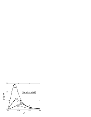
Figure 4: Spectral function $\chi^{\prime\prime}({\bf q},\omega)$ for various wave vectors at $T=0.15t$ and $\delta=0.1$ in comparison with ED data (filled symbols, Ref Prelovsek04 ).

III.3 Spin dynamics in the superconducting state

In the superconducting state the spin-excitation spectrum of high-$T_{\rm c}$ cuprates is dominated by a sharp magnetic peak at the AF wave vector ${\bf Q}$ which is called the resonance mode (RM). It was discovered in the inelastic neutron scattering experiments first in the optimally doped YBa₂Cu₃O_y (YBCO_y) crystal Rossat91 and later on, the RM was found in the Bi-2212 compounds Sidis04 , in the single-layer cuprates Tl₂Ba₂CuO_6+x He02 , HgBa₂CuO_4+δ Yu10 , and in the electron-doped Pr_0.88LaCe_0.12CuO_4-δ superconductor Wilson06 . This demonstrates that the RM is a generic feature of the cuprate superconductors and can be related to spin excitations in a single CuO₂ layer.

The spin-excitation dispersion close to the RM exhibits a peculiar “hour-glass”-like shape with upward and downward dispersions. Whereas the RM energy $E_{\rm r}$ changes with doping, no essential temperature dependence of $E_{\rm r}$ and the upward branch of the dispersion has been found. In the strongly underdoped YBCO crystal only the downward branch is suppressed above $T_{\rm c}$, whereas the upward dispersion and the RM are observed in the normal pseudogap state. So we can conclude that the RM and the upward dispersion are related to the exchange interaction $J\sim 1500$ K and for $\,T\sim T_{c}\ll J$ do not show a noticeable temperature dependence. The downward branch may be explained by inhomogeneous phases related to fluctuating stripe phases with a quasi-one-dimensional order of spins and charges or to a liquid crystal state which are smeared out at $\,T\gtrsim T_{c}$.

To prove this conclusion we consider the spin excitation damping in the superconducting state  Vladimirov11 within the theory formulated in Sec. III.1. We can propose an alternative explanation of the magnetic RM and the upper branch of the dispersion which are driven by the spin gap at the AF wave vector ${\bf Q}=\pi(1,1)$ in the paramagnetic state instead of the superconducting gap $2\Delta$ proposed in the exciton spin-1 scenario (see Sec. III.4).

Figure 5: Spin-excitation damping $\Gamma_{\bf q}$ for (a) $\delta=0.2$ and for (b) $\delta=0.09$ at $T=0$ for the $d$-wave pairing (solid line) and in the normal state (dashed line).

As discussed in the previous section, in the normal state close to AF wave vector the damping $\Gamma_{\bf Q}$ is very small at low doping and low enough temperature. This results in the underdamped spin modes characterized by sharp resonance peaks in $\chi^{\prime\prime}({\bf Q},\omega)$. This property retains in the superconducting state and the RM can be observed even above $T_{\rm c}$ in the underdoped cuprates. In Fig. 5 the spin-excitation damping $\Gamma_{\bf q}=-(1/2)\,\Sigma^{\prime\prime}_{t}({\bf q},\omega=\widetilde{\omega}_{\bf q})$ is shown at $T=0$ for the overdoped case, $\delta=0.2$, Fig. 5 (a) and for the underdoped case, $\delta=0.09$, Fig. 5 (b). The small difference between the damping in the $d$-wave superconducting state and the normal state observed for the full self-energy in both the cases, Eq. (28), confirms that the superconducting gap does not play an essential role in suppressing the damping $\Gamma_{\bf Q}$. The damping in the underdoped region is of the order of magnitude weaker than in the overdoped region. The sharp increase of the damping $\Gamma_{\bf q}$ away from the AF wave-vector ${\bf Q}$ explains the resonance character of spin excitations at ${\bf Q}$.

The temperature dependence of the spectral function $\chi^{\prime\prime}({\bf Q},\omega)$ in the overdoped case $\delta=0.2$ is shown in Fig. 6. It has high intensity at low temperatures, but strongly decreases with temperature and becomes very broad at $T\sim T_{\rm c}$ as found in experiments (see Ref. Bourges98 ). Note, that the shift of the maximum of the peak to lower energies with increasing temperature can be explained just by the increase of the damping as this is usually observed for an overdamped oscillator. In Fig. 7 the temperature dependence of the spectral function $\chi^{\prime\prime}({\bf Q},\omega)$ for the underdoped case $\delta=0.09$ is plotted. Whereas the resonance energy $E_{r}$ decreases with underdoping in comparison with Fig. 6, the intensity of the RM greatly increases in accordance with experiments. The RM intensity decreases with temperature but its energy $E_{r}$ does not change with temperature and is still quite visible at $T=T_{\rm c}$ and even at $T=1.4T_{\rm c}$.

Figure 6: Temperature dependence of the spectral function $\chi^{\prime\prime}({\bf Q},\omega)$ at $\delta=0.2$.

Figure 7: Temperature dependence of the spectral function $\chi^{\prime\prime}({\bf Q},\omega)$ at $\delta=0.09$.

The dispersion of the spectral function for $\delta=0.2$ is shown in Fig. 8 at $T=0$. A strong suppression of the spectral-function intensity away from ${\bf Q}=\pi(1,1)$ explains the resonance-type behavior of the function at low temperatures. This suppression of the intensity is in accord with the sharp increase of the damping away from ${\bf Q}$ shown in Fig. 5. However, the upper branch of the spin-excitation spectrum reminiscent of spin waves is still visible in Fig. 8.

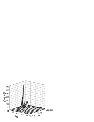
Figure 8: Spectral function $\chi^{\prime\prime}({\bf q},\omega)$ near the wave vector ${\bf Q}=\pi(1,1)$ at $T=0$ for $\delta=0.2$.

Figure 9: Spectral function $\chi^{\prime\prime}({\bf Q},\omega)$ for doping $\delta=0.2$ compared to experimental data for YBCO_6.92, Ref. Bourges98 , at $T=5K$ (squares) and $T=100K$ (circles).

In Fig. 9 we compare our results with the neutron-scattering data for the nearly optimally doped YBCO_6.92 single crystal Bourges98 at $T=5K$ and $T=100K$. In this sample, $T_{\rm c}=91$ K and the RM energy $E_{\rm r}\simeq 40$ meV$=5.1k_{\rm B}\,T_{\rm c}>2\,\Delta_{0}$ (taking $2\Delta_{0}(\delta)=3.52\,k_{\rm B}T_{\rm c}(\delta)$ we have $E_{\rm r}\simeq 2.9\Delta_{0}$). For $\delta=0.2$, our calculations yield $E_{\rm r}=0.12t=38$ meV$=4.8k_{\rm B}\,T_{\rm c}=2.7\,\Delta_{0}$ ($t=0.313$ eV, $k_{\rm B}\,T_{\rm c}=0.025t$ (see Sec. III.1). Since the experimental data are given in arbitrary units (a. u.), our results were scaled to fit the absolute value of the peak at $T=5K$.

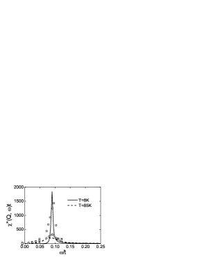
Figure 10: Spectral function $\chi^{\prime\prime}({\bf Q},\omega)$ for doping $\delta=0.09$ compared to experimental data for YBCO_6.5, Ref. Stock04 , at $T=8K$ (squares) and $T=85K$ (circles).

In Fig. 10 our results are compared with the experimental data for the underdoped ortho-II YBCO_6.5 single crystal with $E_{\rm r}=33$ meV$=6.5\,k_{\rm B}T_{\rm c}=3.7\,\Delta_{0}$ at $T=8K$ and $T=85K$ (see Refs. Stock04 ; Stock05 ). For $\delta=0.09$, our theory gives $E_{\rm r}=0.09t=28$ meV$=5.6\,k_{\rm B}\,T_{\rm c}=3.2\,\Delta_{0}$. Here we also scaled our results to fit the absolute value of the peak at $T=8K$. We note a weak temperature dependence of the RM energy observed experimentally and obtained in our calculation. In both compounds the RM energy is larger than the superconducting excitation energy, $2\Delta_{0}$, while in the spin-1 exciton scenario the RM energy $E_{\rm r}$ has to be less than $2\Delta_{0}$. So we obtain a good agreement of our theory with neutron-scattering experiments on YBCO crystals both near the optimal doping and in the underdoped region.

III.4 Comparison with previous theoretical studies

There is a vast literature devoted to experimental and theoretical investigations of spin-excitation spectra and the RM in cuprates (a list of references can be found in reviews Bourges98 ; Sidis04 ; Sidis07 ; Eschrig06 ; Plakida10 and Ref. Vladimirov11 ). To explain the RM in a large number of studies the Fermi-liquid model of itinerant electrons was assumed and the DSS was calculated within the random phase approximation (RPA) for a one-band Hubbard model specified by the Coulomb interaction $U$ or the AF superexchange interaction $J({\bf q})$ (see, e.g., Refs. Norman00 ; Manske01 ; Eremin05 ). Summation of the electron-hole bubble diagrams in the RPA for the self-energy results in a sharp RM formed below the continuum of particle-hole excitations gapped at a threshold energy $\omega_{c}\leq 2\Delta({\bf q}^{*})$ determined by the superconducting $d$-wave gap $2\Delta({\bf q}^{*})$ at a particular wave vector $\,{\bf q}^{*}\,$ on the Fermi surface (FS). In this approach the RM is considered as a particle-hole bound state, usually referred to as the spin-1 exciton.

However, in the spin-1 exciton scenario, a strong temperature dependence of the RM energy is expected below $T_{\rm c}$ due to temperature dependence of the superconducting gap $2\Delta({\bf q}^{*})$ and, hence, the threshold energy $\omega_{c}$. But the temperature dependence of the RM energy was not found in experiments, in particular for the RM at the energy $E_{\rm r}\approx 33$ meV in the YBCO_6.5 crystal Stock04 ; Stock05 . At low temperature, $T\sim 8$ K, the RM revealed a much higher intensity than in optimally doped crystals, and it was also seen at the same energy with less intensity even at $T\simeq 1.4\,T_{\rm c}$ (see Fig. 10).

In the strong correlation limit the Mori projection technique in the equation of motion method for the relaxation function has been used by several groups (see, e.g., Refs. Sega03 ; Prelovsek04 ; Sherman03 ; Sherman06 ; Sega06 ; Prelovsek06 ). However, in several studies of the $t$-$J$ model the contribution of the accompanied spin excitation in the self-energy has been neglected Onufrieva02 or approximated by static or mean-field-type expressions (see, e.g., Refs. Sega03 and  Sherman03 ) which results in the self-energy similar to the RPA formula given by Eq. (38).

That is, in these approximations the spin-excitation contribution was “decoupled” from the particle-hole pair. We can derive the particle-hole bubble approximation from Eq. (28), if we ignore the spin-energy contribution $\omega_{2}$ in comparison with the electron-hole pair energy, or, equivalently, if in the MCA, the time-dependent spin correlation function is approximated by its static value: $\langle S_{\bf-q}^{-}S_{\bf q}^{+}(t)\rangle\simeq\langle S_{\bf-q}^{-}S_{\bf q}^{+}\rangle=C_{\bf q}$. Moreover, excluding the spin-excitation wave-vector ${\bf q}_{2}$ from the wave-vector conservation law, we have ${\bf q}={\bf q}_{1}+{\bf q}_{3}$. As a result of these approximations in Eq. (28), we obtain the self-energy in the form of the particle-hole bubble approximation:

$$\widetilde{\Sigma}_{t}^{\prime\prime}({\bf q},\omega)=-\frac{\pi(2t)^{4}\,}{m({\bf q})\,\omega}\int_{-\infty}^{\infty}d\omega_{1}[n(\omega_{1})-n(\omega_{1}+\omega)]$$

$$\times\frac{1}{N}\,\sum_{{\bf q_{1}}}\,\big{[}\widetilde{\Lambda}^{N}_{{\bf q_{1},q-q_{1}}}\,A^{N}_{\bf q_{1}}(\omega_{1})\,A^{N}_{\bf q-q_{1}}(\omega_{1}+\omega)$$

$$-\widetilde{\Lambda}^{S}_{{\bf q_{1},q-q_{1}}}\,A^{S}_{{\bf q_{1}}\sigma}(\omega_{1})\,A^{S}_{{\bf q-q_{1}}\sigma}(\omega_{1}+\omega)\big{]}.$$ (38)

where the averaged over the spin-excitation wave vector ${\bf q_{2}}$ vertexes are introduced,

$$\widetilde{\Lambda}^{N}_{{\bf q_{1},q_{3}}} = \frac{1}{N}\sum_{{\bf q_{2}}}\,C_{{\bf q}_{2}}[\Lambda^{2}_{\bf q_{1},q_{2},q_{3}}+\Lambda^{2}_{\bf q_{3},q_{2},q_{1}}]\,,$$ (39)

$$\widetilde{\Lambda}^{S}_{{\bf q_{1},q_{3}}} = \frac{2}{N}\sum_{{\bf q_{2}}}\,C_{{\bf q}_{2}}{\Lambda}_{\bf q_{1},q_{2},q_{3}}{\Lambda}_{\bf q_{3},q_{2},q_{1}}.$$ (40)

In the approximation (38) only the opening of a superconducting gap in the particle-hole excitation can suppress the damping of spin excitations due to the decay into particle-hole pairs which may result in the RM. Figure 11 shows the spectral function $\,\chi^{\prime\prime}({\bf q},\omega)\,$ and the damping $\Gamma({\bf Q},\omega)$ using Eq. (38). To compare these functions with those calculated in Ref. Sega03 , we adopt the electron dispersion used in Ref. Sega03 , $\,\varepsilon_{\bf q}^{eff}=-4\,t_{eff}\gamma_{\bf q}-4\,t^{\prime}_{eff}\cos q_{x}\cos q_{y}\,$ with $t_{eff}=0.3t$ and $t^{\prime}_{eff}=-0.1t\,$ and take the gap parameter $\,\Delta_{0}=0.1t$. The obtained results are quite close to those shown in Fig. 1 of Ref. Sega03 (where $\chi_{zz}^{\prime\prime}({\bf q},\omega)=(1/2)\chi^{\prime\prime}({\bf q},\omega)\,$ is plotted). At $T=0$, we observe a much narrower RM, but with a lower intensity in comparison with the RM calculated with the full self-energy, Eq. (28), as shown in Fig. 6. The energy $E_{\rm r}$ of the RM shown Fig. 11(a) noticeably decreases with increasing temperature, contrary to a negligible shift of the RM shown in Fig. 6 for $T=0.4T_{\rm c}$. This comparison demonstrates that in the particle-hole bubble approximation the superconducting gap plays a crucial role in the occurrence of the RM with $E_{\rm r}(T)<2\Delta(T)$, while in the full self-energy (28) the superconducting gap and details of the electron dispersion are less important. Note that the damping in the normal state for the reduced self-energy, Eq. (38), is the order of magnitude larger than for the full self-energy, Eq. (28) (see Fig. 11(b)).

Figure 11: (a) Spectral function $\chi^{\prime\prime}({\bf Q},\omega)$ and (b) spin-excitation damping $\Gamma({\bf Q},\omega)$ calculated in the particle-hole bubble approximation, Eq. (38), at $\delta=0.2$ for the $d$-wave pairing ($\Delta_{0}=0.1t$ taken from Ref. Sega03 ) at $T=0$ (solid line) and $T=0.4T_{\rm c}$ (dotted line), and for the normal state at $T=0$ (dashed line) and $T=T_{\rm c}$ (dash-dotted line).

This difference can be explained as follows. Whereas in the particle-hole bubble approximation given by Eq. (38) the spin excitation with the energy $\omega$ at the wave vector ${\bf Q}$ can decay only into a particle-hole pair with the energy $\omega({\bf Q})=E_{\bf Q+q}+E_{\bf q}$, in a more general process described by Eq. (28) an additional spin excitation participates in the scattering. In the limit $T\to 0$, the decay process in this case is governed by another energy-conservation law, $\omega({\bf Q})=E_{\bf q_{3}}+E_{\bf q_{1}}+\widetilde{\omega}_{\bf q_{2}}$ where the largest contribution from the spin excitation comes from $\widetilde{\omega}_{\bf q_{2}}\simeq\widetilde{\omega}_{\bf Q}$ due to the factor $\,m({\bf q}_{2})\,$ (18) in $B({\bf q}_{2})$ (37) in Eq. (28). This energy-momentum conservation law strongly reduces the phase space for the decay and suppresses the damping of the initial spin excitation with the energy $\omega({\bf Q})$. In fact, the occurrence of an additional spin excitation in the scattering process with the finite energy $\widetilde{\omega}_{\bf Q}$ plays a role similar to the superconducting gap in the excitation of the particle-hole pair in Eq. (38). Therefore, the damping at low temperatures ($k_{\rm B}\,T\ll\widetilde{\omega}_{\bf Q}\sim E_{\rm r}$) appears to be small even in the normal state as demonstrated in Fig. 6. In the case of the particle-hole relaxation, the condition for the occurrence of the RM, $\,\omega({\bf Q})=E_{\bf q+Q}+E_{\bf q}\leq 2\Delta({\bf q}^{*})$, imposes a strong restriction on the shape of the FS which should cross the AF Brillouin zone to accommodate the scattering vector ${\bf Q}$ and the vector ${\bf q}^{*}$ on the FS. In the case of the full self-energy, Eq. (28), the energy-momentum conservation law for three quasipartricles does not impose such strict limitations.

IV Kinematical spin-fluctuation mechanism of pairing in cuprates

IV.1 General formulation

Hamiltonian. In this section we consider a more general than in Ref. (1) extended Hubbard model

$$H = \varepsilon_{1}\sum_{i,\sigma}X_{i}^{\sigma\sigma}+\varepsilon_{2}\sum_{i}X_{i}^{22}+\sum_{i\neq j,\sigma}\,t_{ij}\,\bigl{\{}X_{i}^{\sigma 0}\,X_{j}^{0\sigma}$$ (41)

$$+ X_{i}^{2\sigma}X_{j}^{\sigma 2}+\sigma\,(X_{i}^{2\bar{\sigma}}X_{j}^{0\sigma}+{\rm H.c.})\bigr{\}}+H_{c,ep},$$

which includes also electron-phonon interaction $g_{ij}$ defined by the Hamiltonian

$$H_{c,ep} = \frac{1}{2}\sum_{i\neq j}\,V_{ij}N_{i}N_{j}+\sum_{i,j}\,g_{ij}N_{i}\,u_{j},$$ (42)

where $u_{j}$ describes an atomic displacement on the lattice site $j$ for a particular phonon mode. More generally, the electron-phonon interaction can be written as a sum $\sum_{\nu}g^{\nu}_{i,j}u_{j}^{\nu}$ over the normal modes $\nu$.

We emphasize here that the Hubbard model (41) does not involve a dynamical coupling of electrons (holes) to fluctuations of spins or charges. Its role is played by the kinematical interaction caused by the complicated commutation relations (9), as was already noted by Hubbard Hubbard65 . For example, the equation of motion for the HO $\,X_{i}^{\sigma 2}=a^{{\dagger}}_{i\sigma}a_{i\sigma}a_{i\bar{\sigma}}\,$ for the model (41) reads:

$$i\frac{d}{dt}X_{i}^{\sigma 2} = [X_{i}^{\sigma 2},H]=(\varepsilon_{1}+U)\,X_{i}^{\sigma 2}\,$$ (43)

$$+ \sum_{l,\sigma^{\prime}}\!\left(t_{il}^{22}B_{i\sigma\sigma^{\prime}}^{22}X_{l}^{\sigma^{\prime}2}-\sigma t^{21}_{il}B_{i\sigma\sigma^{\prime}}^{21}X_{l}^{0\bar{\sigma}^{\prime}}\right)$$

$$- \sum_{l}X_{i}^{02}\left(t^{11}_{il}X_{l}^{\sigma 0}+\sigma t^{21}_{il}X_{l}^{2\bar{\sigma}}\right)$$

$$+ \sum_{l}X_{i}^{\sigma 2}(V_{il}\,N_{l}+g_{il}\,u_{l}).$$

Here $B_{i\sigma\sigma^{\prime}}^{\eta\zeta}$ are the Bose-like operators,

$$B_{i\sigma\sigma^{\prime}}^{22} = (X_{i}^{22}+X_{i}^{\sigma\sigma})\,\delta_{\sigma^{\prime}\sigma}+X_{i}^{\sigma\bar{\sigma}}\,\delta_{\sigma^{\prime}\bar{\sigma}}$$

$$= (N_{i}/2+\sigma\,S_{i}^{z})\,\delta_{\sigma^{\prime}\sigma}+S_{i}^{\sigma}\,\delta_{\sigma^{\prime}\bar{\sigma}},$$

$$B_{i\sigma\sigma^{\prime}}^{21} = (N_{i}/2+\sigma S_{i}^{z})\,\delta_{\sigma^{\prime}\sigma}-S_{i}^{\sigma}\,\delta_{\sigma^{\prime}\bar{\sigma}}.$$ (45)

We see that the hopping amplitudes here depend on the number and spin operators due to the kinematical interaction of electrons with spin and charge fluctuations. In phenomenological spin-fermion models, a dynamical coupling of electrons with spin fluctuations is specified by fitting parameters, while in Eq. (43) the interaction is determined by the hopping energy $t_{ij}$ fixed by the electronic dispersion.

Dyson equation. To consider superconducting pairing in the model (41), we introduce the two-time thermodynamic GF Zubarev60 expressed in terms of the four-component Nambu operators, $\,\hat{X}_{i\sigma}$ and $\,\hat{X}_{i\sigma}^{\dagger}=(X_{i}^{2\sigma}\,\,X_{i}^{\bar{\sigma}0}\,\,X_{i}^{\bar{\sigma}2}\,\,X_{i}^{0\sigma})\,$:

$${\sf G}_{ij\sigma}(t-t^{\prime}) = -i\theta(t-t^{\prime})\langle\{\hat{X}_{i\sigma}(t),\hat{X}_{j\sigma}^{\dagger}(t^{\prime})\}\rangle$$ (46)

$$\equiv \langle\!\langle\hat{X}_{i\sigma}(t)\mid\hat{X}_{j\sigma}^{\dagger}(t^{\prime})\rangle\!\rangle,$$

where $\{A,B\}=AB+BA$, $A(t)=\exp(iHt)A\exp(-iHt)$, and $\theta(x)=1$ for $x>0$ and $\theta(x)=0$ for $x<0$. The Fourier representation in $({\bf k},\omega)$-space is defined by the relations:

$${\sf G}_{ij\sigma}(t-t^{\prime}) = \frac{1}{2\pi}\int_{-\infty}^{\infty}dte^{-i(t-t^{\prime})}{\sf G}_{ij\sigma}(\omega),$$ (47)

$${\sf G}_{ij\sigma}(\omega) = \frac{1}{N}\,\sum_{\bf k}\exp[i{\bf k(i-j)}]{\sf G}_{\sigma}({\bf k},\omega).$$ (48)

The GF (48) is convenient to write in the matrix form

$${\sf G}_{\sigma}({\bf k},\omega)={\hat{G}_{\sigma}({\bf k},\omega)\quad\quad\hat{F}_{\sigma}({\bf k},\omega)\choose\hat{F}_{\sigma}^{\dagger}({\bf k},\omega)\quad-\hat{G}_{\bar{\sigma}}(-{\bf k},-\omega)},$$ (49)

where the normal $\hat{G}_{\sigma}({\bf k},\omega)$ and anomalous (pair) $\hat{F}_{\sigma}({\bf k},\omega)$ GFs are $2\times 2$ matrices for two Hubbard subbands:

$$\hat{G}_{\sigma}({\bf k},\omega)=\langle\!\langle\left(\begin{array}[]{c}X_{\bf k}^{\sigma 2}\\ X_{\bf k}^{0\bar{\sigma}}\\ \end{array}\right)\mid X_{\bf k}^{2\sigma}X_{\bf k}^{\bar{\sigma}0}\rangle\!\rangle_{\omega},$$ (50)

$$\hat{F}_{\sigma}({\bf k},\omega)=\langle\!\langle\left(\begin{array}[]{c}X_{\bf k}^{\sigma 2}\\ X_{\bf k}^{0\bar{\sigma}}\\ \end{array}\right)\mid X_{-\bf k}^{\bar{\sigma}2}X_{-\bf k}^{0\sigma}\rangle\!\rangle_{\omega}.$$ (51)

To calculate the GF (46) we use the equation of motion method. Differentiating the GF with respect to time $t$ we obtain the equation for the Fourier representation (47)

$$\omega{\sf G}_{ij\sigma}(\omega)=\delta_{ij}{\sf Q}+\langle\!\langle[\hat{X}_{i\sigma},H]\mid\hat{X}_{j\sigma}^{\dagger}\rangle\!\rangle_{\omega}\,.$$ (52)

Here the correlation function ${\sf Q}=\langle\{\hat{X}_{i\sigma},\hat{X}_{i\sigma}^{\dagger}\}\rangle=\hat{\tau}_{0}\times\hat{Q}\,$ where $\,\hat{Q}=\left(\begin{array}[]{cc}Q_{2}&0\\ 0&Q_{1}\end{array}\right)\,$ and $\hat{\tau}_{0}$ is the $2\times 2$ unit matrix. The spectral weights of the Hubbard subbands in the paramagnetic state $\,Q_{2}=\langle X_{i}^{22}+X_{i}^{\sigma\sigma}\rangle=n/2\,$ and $\,Q_{1}=\langle X_{i}^{00}+X_{i}^{\bar{\sigma}\bar{\sigma}}\rangle=1-Q_{2}\,$ depend on the average occupation number of holes (5). In the $\,{\sf Q}$ matrix we neglect anomalous averages of the type $\langle X_{i}^{02}\rangle$ which are irrelevant for the $d$-wave pairing Adam07 .

To introduce the zero-order quasiparticle (QP) excitation energy we use the Mori-type projection operator method Mori65 ; Plakida11 . In this approach, the many-particle operator $\hat{Z}_{i\sigma}=[\hat{X}_{i\sigma},H]$ in (52) is written as a sum of a linear part and an irreducible part $\hat{Z}_{i\sigma}^{(ir)}$ orthogonal to $\hat{X}_{j\sigma}^{\dagger}$:

$$\hat{Z}_{i\sigma}=[\hat{X}_{i\sigma},H]=\sum_{l}{\sf E}_{il\sigma}\hat{X}_{l\sigma}+\hat{Z}_{i\sigma}^{(\rm ir)}.$$ (53)

From the orthogonality condition, $\langle\{\hat{Z}_{i\sigma}^{(\rm ir)},\,\hat{X}_{j\sigma}^{\dagger}\}\rangle=0$, we obtain the excitation energy in the GMFA which is given by the time-independent matrix of correlation functions:

$${\sf E}_{ij\sigma} = \langle\{[\hat{X}_{i\sigma},H],\hat{X}_{j\sigma}^{\dagger}\}\rangle{\sf Q}^{-1}.$$ (54)

The corresponding zero-order GF reads

$${\sf G}^{0}_{\sigma}({\bf k},\omega)=\Bigl{(}\omega\tilde{\tau}_{0}-{\sf E}_{\sigma}({\bf k})\Bigr{)}^{-1}{\sf Q}\,,$$ (55)

where $\tilde{\tau}_{0}$ is the $4\times 4$ unit matrix. The spectrum of QP excitations in the GMFA is given by the Fourier component of the matrix (54):

$${\sf E}_{\sigma}({\bf k}) = \frac{1}{N}\sum_{\bf k}\exp[i{\bf k(i-j)}]\langle\{[\hat{X}_{i\sigma},H],\hat{X}_{j\sigma}^{\dagger}\}\rangle{\sf Q}^{-1}$$ (58)

$$= \left(\begin{array}[]{cc}\hat{\varepsilon}({\bf k})&\hat{\Delta}_{\sigma}({\bf k})\\ \hat{\Delta}_{\sigma}^{*}({\bf k})&-\hat{\varepsilon}({\bf k})\end{array}\right),$$

where $\hat{\varepsilon}({\bf k})$ and $\hat{\Delta}_{\sigma}({\bf k})$ are the normal and anomalous parts of the energy matrix.

To calculate the multiparticle GF $\,\langle\langle\hat{Z}_{i\sigma}^{(\rm ir)}(t)\mid\hat{X}_{j\sigma}^{\dagger}(t^{\prime})\rangle\rangle\,$ in (52) we differentiate it with respect to the second time $t^{\prime}$ and apply the same projection procedure as in (53). This results in the equation for the GF (52) in the form,

$${\sf G}_{\sigma}({\bf k},\omega)={\sf G}^{0}_{\sigma}({\bf k},\omega)+{\sf G}^{0}_{\sigma}({\bf k},\omega)\,{\sf T}_{\sigma}({\bf k},\omega)\,{\sf G}^{0}_{\sigma}({\bf k},\omega),$$ (59)

where the scattering matrix

$${\sf T}_{\sigma}({\bf k},\omega)={\sf Q}^{-1}\,\langle\!\langle{\hat{Z}}_{{\bf k}\sigma}^{(\rm ir)}\!\mid\!{\hat{Z}}_{{\bf k}\sigma}^{(\rm ir)\dagger}\rangle\!\rangle_{\omega}\;{\sf Q}^{-1}.$$ (60)

Now we can introduce the self-energy operator ${\sf\Sigma}_{\sigma}({\bf q},\omega)$ as the proper part (pp) of the scattering matrix (60) which has no parts connected by the zero-order GF (55) according to the equation: ${\sf T}={\sf\Sigma}+{\sf\Sigma}\,{\sf G}^{0}\,{\sf T}$. The definition of the proper part of the scattering matrix (60) is equivalent to an introduction of a projected Liouvillian superoperator for the memory function in the conventional Mori technique Mori65 .

Using the self-energy operator instead of the scattering matrix in Eq. (59) we obtain the Dyson equation for the GF (46):

$${\sf G}_{\sigma}({\bf k},\omega)=\left[\omega\tilde{\tau}_{0}-{\sf E}_{\sigma}({\bf k})-{\sf Q}{\sf\Sigma}_{\sigma}({\bf k},\omega)\right]^{-1}{\sf Q},$$ (61)

where the self-energy operator is given by

$${\sf Q}{\sf\Sigma}_{\sigma}({\bf k},\omega)=\langle\!\langle{\hat{Z}}_{{\bf k}\sigma}^{(\rm ir)}\!\mid\!{\hat{Z}}_{{\bf k}\sigma}^{(\rm ir)\dagger}\rangle\!\rangle^{(\rm pp)}_{\omega}\;{\sf Q}^{-1}.$$ (62)

Dyson equation (61) with the zero-order QP excitation energy (58) and the self-energy (62) gives an exact representation for the GF (46). The self-energy takes into account processes of inelastic scattering of electrons (holes) on spin and charge fluctuations due to the kinematical interaction and the dynamic intersite CI and the electron-phonon interaction.

The self-energy operator (62) can be written in the same matrix form as the GF (49):

$${\sf Q}{\sf\Sigma}_{\sigma}({\bf k},\omega)={\hat{M}_{\sigma}({\bf k},\omega)\quad\quad\hat{\Phi}_{\sigma}({\bf k},\omega)\choose\hat{\Phi}_{\sigma}^{\dagger}({\bf k},\omega)\quad-\hat{M}_{\bar{\sigma}}({\bf k},-\omega)}{\sf Q}^{-1}\,,$$ (63)

where the matrices $\hat{M}$ and $\hat{\Phi}$ denote the corresponding normal and anomalous (pair) components of the self-energy operator.

The system of equations for the $(4\times 4)$ matrix GF (49) and the self-energy (63) can be reduced to a system of equations for the normal ${\hat{G}}_{\sigma}({\bf k},\omega)$ and the pair ${\hat{F}}_{\sigma}({\bf k},\omega)$ matrix components. Using representations for the energy matrix (58) and the self-energy (63), we derive for these components the following system of matrix equations:

$${\hat{G}}({\bf k},\omega)=\Bigl{\{}\hat{G}_{N}({\bf k},\omega)^{-1}$$ (65)

$$+ \hat{\varphi}_{\sigma}({\bf k},\omega)\,\hat{G}_{N}({\bf k},-\omega)\,\hat{\varphi}^{*}_{\sigma}({\bf k},\omega)\Bigr{\}}^{-1}\,\hat{Q},$$

$${\hat{F}}_{\sigma}({\bf k},\omega)=-\hat{G}_{N}({\bf k},-\omega)\,\hat{\varphi}_{\sigma}({\bf k},\omega)\,\hat{G}({\bf k},\omega),$$

where we introduced the normal state GF

$${\hat{G}}_{N}({\bf k},\omega) = \Bigl{(}\omega\hat{\tau}_{0}-\hat{\varepsilon}({\bf k})-\hat{M}({\bf k},\omega)/\hat{Q}\Bigr{)}^{-1},$$ (66)

and the superconducting gap function

$${\hat{\varphi}}_{\sigma}({\bf k},\omega) = \hat{\Delta}_{\sigma}({\bf k})+\hat{\Phi}_{\sigma}({\bf k},\omega)/\hat{Q}.$$ (67)

The system of equations for the normal GFs (65), (66), the anomalous GF (65) and the gap equation (67) should be solved self-consistently for the multiparticle GFs in the self-energy operator (63) as discussed below.

IV.2 Generalized mean-field approximation

The superconducting pairing in the Hubbard model already occurs in the MFA and is caused by the kinetic superexchange interaction as in the $t$–$J$ model Anderson87 . Therefore, it is reasonable to consider at first the MFA described by the zero-order GF (55). The energy matrix (54) is calculated using the commutation relations (6) for the HOs. The normal part $\hat{\varepsilon}({\bf k})\,$ of the energy matrix (58) after diagonalization determines the QP spectrum in two Hubbard subbands in the GMFA (for detail see Plakida07 ):

$${\varepsilon}_{1,2}({\bf k}) = ({1}/{2})[\omega_{2}({\bf k})+\omega_{1}({\bf k})]\mp({1}/{2})\Lambda({\bf k}),$$ (68)

$${\omega}_{\iota}({\bf k}) = 4t\,\alpha_{\iota}\gamma({\bf k})+4\,\beta_{\iota}\,t^{\prime}\gamma^{\prime}({\bf k})+4\,\beta_{\iota}\,t^{\prime\prime}\gamma^{\prime\prime}({\bf k})$$ (69)

$$+ \omega^{(c)}_{\iota}({\bf k})+U\delta_{\iota,2}-\mu,\quad(\iota=1,2)$$

$$\Lambda({\bf k}) = \{[\omega_{2}({\bf k})-\omega_{1}({\bf k})]^{2}+4W({\bf k})^{2}\}^{1/2},$$

$$W({\bf k}) = 4t\,\alpha_{12}\gamma({\bf k})+4t^{\prime}\,\beta_{12}\gamma^{\prime}({\bf k})+4t^{\prime\prime}\,\beta_{12}\gamma^{\prime\prime}({\bf k}).$$

Here the hopping parameter is defined by the expression:

$$t_{ij} = (1/N)\,\sum_{\bf k}\exp[i{\bf k(i-j)}]\,t({\bf k}),$$ (70)

$$t({\bf k}) = 4t\,\gamma({\bf k})+4t^{\prime}\,\gamma^{\prime}({\bf k})+4t^{\prime\prime}\,\gamma^{\prime\prime}({\bf k}).$$ (71)

which are equal to $t\,$ for the nearest neighbors (nn) sites $a_{1}=(\pm a_{x},\pm a_{y})$, $\,t^{\prime}\,$ – for the next nearest neighbors (nnn) sites $a_{d}=\pm(a_{x}\pm a_{y})$, and $\,t^{\prime\prime}\,$ – for the nnn sites $\,a_{2}=(\pm 2a_{x},\pm 2a_{y})$. The corresponding ${\bf k}$-dependent functions are: $\,\gamma({\bf k})=(1/2)(\cos k_{x}+\cos k_{y}),\;\gamma^{\prime}({\bf k})=\,\cos k_{x}\cos k_{y}\,$, and $\;\gamma^{\prime\prime}({\bf k})=(1/2)(\cos 2k_{x}+\cos 2k_{y})$ (the lattice constants $a_{x}=a_{y}$ are put to unity).

The kinematical interaction for the HOs results in renormalization of the spectrum (68) determined by the parameters: $\,\alpha_{\iota}=Q_{\iota}[1+{C_{1}}/{Q^{2}_{\iota}}],\,\beta_{\iota}=Q_{\iota}[1+{C_{2}}/{Q^{2}_{\iota}}]\,$, $\,\alpha_{12}=\sqrt{Q_{1}Q_{2}}[1-{C_{1}}/{Q_{1}Q_{2}}],\,\beta_{12}=\sqrt{Q_{1}Q_{2}}[1-{C_{2}}/{Q_{1}Q_{2}}]\,$. In addition to the conventional Hubbard I renormalization given by $Q_{1},\,Q_{2}$ parameters an essential renormalization is caused by the AF spin correlation functions for the nn and the nnn sites, respectively:

$$C_{1}=\langle{\bf S}_{i}{\bf S}_{i+a_{1}}\rangle,\quad C_{2}=\langle{\bf S}_{i}{\bf S}_{i+a_{d}(a_{2})}\rangle.$$ (72)

These functions strongly depend on doping resulting in a considerable variation of the electronic spectrum as shown later and discussed in detail in Ref. Plakida07 .

The contribution from the CI $V_{ij}$ in (69) is given by

$$\omega^{(c)}_{1(2)}({\bf k})=\frac{1}{N}\sum_{\bf q}V({\bf k-q})N_{1(2)}({\bf q}),$$ (73)

where $N_{1}({\bf q})=\langle X_{\bf q}^{0\bar{\sigma}}X_{\bf q}^{\bar{\sigma}0}\rangle/Q_{1}\,$ and $\,N_{2}({\bf q})=\langle X_{\bf q}^{\sigma 2}X_{{}_{\bf q}}^{2\sigma}\rangle/Q_{2}\,$ are occupation numbers in the single-particle and two-particle subbands, respectively and $V({\bf q})$ is the Fourier transform of intersite CI $V_{ij}$.

The anomalous component $\,\hat{\Delta}_{\sigma}({\bf k})\,$ of the matrix (58) determines the superconduction gap in the GMFA. Considering the singlet $d$-wave pairing, we calculate the intersite pair correlation functions. The diagonal matrix components are given by the equations:

$$\Delta_{ij\sigma}^{22}Q_{2}=-\sigma\,t_{ij}^{21}\langle X_{i}^{02}N_{j}\rangle-V_{ij}\langle X_{i}^{\sigma 2}\,X_{j}^{\bar{\sigma}2}\rangle,$$ (74)

$$\Delta_{ij\sigma}^{11}Q_{1}=\sigma\,t_{ij}^{12}\langle N_{j}X_{i}^{02}\rangle-V_{ij}\langle X_{i}^{0\bar{\sigma}}X_{j}^{0\sigma}\rangle.$$ (75)

Here we used the notation $t_{ij}^{12}$ for the interband hopping parameters to emphasize that the kinematical pairing $\langle X_{i}^{02}N_{j}\rangle$ is mediated by the interband hopping. In terms of the Fermi operators $a_{i\sigma}=X_{i}^{0\sigma}+\sigma X_{i}^{\bar{\sigma}2}$, the pair correlation function in (74) can be written as $\,\langle X_{i}^{02}N_{j}\rangle=\langle X_{i}^{0\downarrow}X_{i}^{\downarrow 2}N_{j}\rangle=\langle a_{i\downarrow}\,a_{i\uparrow}N_{j}\rangle$. This representation shows that the kinematical pairing occurs on a single lattice site but in two Hubbard subbands Plakida03 . The correlation function $\,\langle X_{i}^{02}N_{j}\rangle$ can be calculated directly from the GF $\,L_{ij}(t-t^{\prime})=\langle\langle X_{i}^{02}(t)\mid N_{j}(t^{\prime})\rangle\rangle\,$ without any decoupling approximation as shown in Ref. Plakida03 . In particular, under hole doping, $n=1+\delta>1$, the pair correlation function in the two-site approximation, as shown in Ref. Plakida03 , reads:

$$\langle X_{i}^{02}N_{j}\rangle=-\frac{4t_{ij}^{12}}{U}\sigma\,\langle X_{i}^{\sigma 2}X_{j}^{\bar{\sigma}2}\rangle.$$ (76)

As a result, the equation for the superconducting gap in (74) can be written as

$$\Delta^{22}_{ij\sigma}=(J_{ij}-V_{ij})\,\langle X_{i}^{\sigma 2}X_{j}^{\bar{\sigma}2}\rangle/Q_{2},$$ (77)

where $\,J_{ij}={4\,(t_{ij}^{12})^{2}}/{U}$ is the AF superexchange interaction. A similar equation holds for the gap in the one-hole subband: $\,\Delta_{ij\sigma}^{11}=(J_{ij}-V_{ij})\,\langle X_{i}^{0\bar{\sigma}}X_{j}^{0\sigma}\rangle/Q_{1}\,$. We thus conclude that the pairing in the Hubbard model in the GMFA is similar to the superconductivity in the $t$–$J$ model mediated by the AF superexchange interaction $J_{ij}$ induced by the kinematical interaction for the interband hopping as in the $t$-$J$ model Anderson87 .

IV.3 Self-energy operator

To determine the self-energy matrix we should calculate many-particle GFs in Eq. (63). Since the diagram technique for HOs is very complicated and can be used effectively only for the lowest order diagrams in the Hubbard model (see, e.g., Refs. Zaitsev87 ; Izyumov91 ) we consider a more simple technique based on the two-time decoupling of multiparticle correlation functions in the projection operator method Plakida11 . In this method the SCBA is used which is equivalent to the noncrossing approximation in the diagram technique. In this approximation, a propagation of Fermi-type excitations described by operators $\,X_{l}^{\sigma^{\prime}2},\,$ and Bose-type excitations described by operators $B_{i\sigma\sigma^{\prime}}$ on different lattice sites, $\,l\neq i$, is assumed to be independent. Therefore, the time-dependent multiparticle correlation functions in the self-energy operators (63) can be written as a product of fermionic and bosonic correlation functions,

$$\langle X_{l^{\prime}}^{2\sigma^{\prime\prime}}B_{j\sigma\sigma^{\prime\prime}}^{\dagger}|B_{i\sigma\sigma^{\prime}}(t)X_{l}^{\sigma^{\prime}2}(t)\rangle$$

$$= \delta_{\sigma^{\prime},\sigma^{\prime\prime}}\langle X_{l^{\prime}}^{2\sigma^{\prime}}X_{l}^{\sigma^{\prime}2}(t)\rangle\langle B_{j\sigma\sigma^{\prime}}^{\dagger}|B_{i\sigma\sigma^{\prime}}(t)\rangle,$$

$$\langle X_{l^{\prime}}^{\bar{\sigma}^{\prime\prime}2}B_{j\bar{\sigma}\bar{\sigma}^{\prime\prime}}|B_{i\sigma\sigma^{\prime}}(t)X_{l}^{\sigma^{\prime}2}(t)\rangle$$

$$= \delta_{\sigma^{\prime},\sigma^{\prime\prime}}\langle X_{l^{\prime}}^{\bar{\sigma}^{\prime}2}X_{l}^{\sigma^{\prime}2}(t)\rangle\,\langle B_{j\bar{\sigma}\bar{\sigma}^{\prime}}B_{i\sigma\sigma^{\prime}}(t)\rangle\,.$$ (79)

The time-dependent correlation functions are calculated self-consistently using the corresponding GFs.

In particular, the normal and anomalous diagonal components of the self-energy for the two-particle subband are determined by the expressions

$$M^{22}({\bf k},\omega) = \frac{1}{N}\sum_{\bf q}\int\limits_{-\infty}^{+\infty}\!\!{\rm d}z\,K^{(+)}(\omega,z|{\bf q},{\bf k-q})$$

$$\times \Big{\{}-({1}/{\pi})\mbox{Im}\left[G^{22}({\bf q},z)+G^{11}({\bf q},z)\right]\Big{\}},\quad$$

$$\Phi_{\sigma}^{22}({\bf k},\omega) = \frac{1}{N}\sum_{\bf q}\int\limits_{-\infty}^{+\infty}\!\!{\rm d}z\,K^{(-)}(\omega,z|{\bf q},{\bf k-q})$$

$$\times \Big{\{}-({1}/{\pi})\mbox{Im}\left[F_{\sigma}^{22}({\bf q},z)-F_{\sigma}^{11}({\bf q},z)\right]\Big{\}},\quad$$

where $G^{\alpha\alpha}({\bf q},z)$ and $F_{\sigma}^{\alpha\alpha}({\bf q},z)$ are given by the diagonal components of the matrices (65), (65). Similar expressions hold for the self-energy components $M^{11}({\bf k},\omega)$ and $\Phi_{\sigma}^{11}({\bf k},\omega)$ for the one-particle subband (see Ref. Plakida97 ). Note, that in the paramagnetic normal state the GF (65) and the self-energy (IV.3) do not depend on the spin $\sigma$.

The kernel of the integral equations (IV.3), (IV.3) has a form, similar to the strong-coupling Migdal-Eliashberg theory Migdal58 ; Eliashberg60 :

$$K^{(\pm)}(\omega,z|{\bf q},{\bf k-q})=\frac{1}{\pi}\int\limits_{-\infty}^{+\infty}{\rm d}\Omega\,\frac{1+N(\Omega)-n(z)}{\omega-z-\Omega}$$ (82)

$$\times \Big{\{}|t({\bf q})|^{2}{\rm Im}\chi_{sf}({\bf k-q},\Omega)$$

$$\pm \Big{[}\left(|V({\bf k-q})|^{2}+|t({\bf q})|^{2}/4\right){\rm Im}\,\chi_{cf}({\bf k-q},\Omega)$$

$$+ |g({\bf k-q})|^{2}{\rm Im}\chi_{ph}({\bf k-q},\Omega)\Big{]}\;\Big{\}}.$$

The spectral densities of bosonic excitations are determined by the dynamic susceptibility for spin $(sf)$, number (charge) $(cf)$, and lattice (phonon) $(ph)$ fluctuations

$$\chi_{sf}({\bf q},\omega) = -\langle\!\langle{\bf S_{q}|S_{-q}}\rangle\!\rangle_{\omega},$$ (83)

$$\chi_{cf}({\bf q},\omega) = -\langle\!\langle\delta N_{\bf q}|\delta N_{-\bf q}\rangle\!\rangle_{\omega},$$ (84)

$$\chi_{ph}({\bf q},\omega) = -\langle\!\langle u_{\bf q}|u_{-\bf q}\rangle\!\rangle_{\omega},$$ (85)

which are defined in terms of the commutator GFs Zubarev60 for the spin ${\bf S_{q}}$, number $\delta N_{\bf q}=N_{\bf q}-\langle N_{\bf q}\rangle$, and lattice displacement (phonon) $u_{\bf q}$ operators.

In the SCBA (IV.3), (79), vertex corrections to the kinematical interaction $\,t({\bf q})\,$ of electrons with spin- and charge-fluctuations (83), (84) induced by the intraband hopping are neglected. It is assumed that the system is far away from a charge instability or a stripe formation and charge-fluctuations give a small contribution to the pairing. The largest contribution from spin fluctuations comes from wave vectors close the AF wave vector ${\bf Q}=\pi\,(1,1)$ where their energy $\omega_{s}({\bf Q})$ is much smaller than the Fermi energy, $\,\omega_{s}({\bf Q})/E_{\rm F}\ll 1\,$ (see, e.g., Vladimirov09 ). Therefore, vertex corrections to the kinematical interaction should be small as in Eliashberg theory Eliashberg60 for electron interaction with phonons, where $\,\omega_{ph}/E_{\rm F}\ll 1\,$. Consequently, the SCBA for the self-energy and the GFs calculated self-consistently is quite reliable and makes it possible to examine the strong coupling regime which is essential in study of renormalization of the QP spectrum and the superconducting pairing as shown in Refs. Plakida07 ; Plakida13 and discussed later.

V Results and discussion

V.1 Self-consistent system of equations

The self-consistent system of equations for the diagonal components of normal GFs (65), (66) and the self-energy (IV.3) can be written in the form Plakida07 :

$${G}^{11(22)}_{N}({\bf k},\omega) = [1-b({\bf k})]{G}_{1(2)}({\bf k},\omega)$$ (86)

$$+ b({\bf k}){G}_{2(1)}({\bf k},\omega),$$

where the hybridization parameter $\,b({\bf k})=[{\varepsilon}_{2}({\bf k})-\omega_{2}({\bf k})]/[{\varepsilon}_{2}({\bf k})-{\varepsilon}_{1}({\bf k})]\,$. The two subband GFs in Eq. (86) in the imaginary frequency representation, $i\omega_{n}=i\pi T(2n+1)$, $n=0,\pm 1,\pm 2,...\,$, take the form:

$$\{G_{1(2)}({\bf k},\omega_{n})\}^{-1}=i\omega_{n}-{\varepsilon}_{1(2)}({\bf k})-\Sigma({\bf k},\omega_{n}).$$ (87)

The self-energy $\Sigma({\bf k},\omega)$ can be approximated by the same function for two subbands:

$${\Sigma}({\bf k},\omega_{n}) = -\frac{T}{N}\sum_{\bf q}\sum_{m}\lambda^{(+)}({\bf q,k-q}\mid\omega_{n}-\omega_{m})$$ (88)

$$\times [{G}_{1}({\bf q},\omega_{m})+{G}_{2}({\bf q},\omega_{m})]$$

$$\equiv i\omega_{n}\,[1-Z({\bf k},\omega_{n})]+X({\bf k},\omega_{n}).$$

Density of states (DOS) is determined by

$$A(\omega)=\frac{1}{N}\sum_{\bf k}\,{A}({\bf k},\omega),$$ (89)

where the spectral function reads

$${A}({\bf k},\omega) = [Q_{1}+P({\bf k})]{A}_{1}({\bf k},\omega)$$ (90)

$$+ [Q_{2}-P({\bf k})]{A}_{2}({\bf k},\omega),$$

$$A_{1(2)}({\bf k},\omega) = -({1}/{\pi})\,{\rm Im}{G}_{1(2)}({\bf k},\omega).$$

Here the hybridization parameter $\,P({\bf k})=(n-1)b({\bf k})-2\sqrt{Q_{1}\,Q_{2}}$ $[W({\bf k})/\Lambda({\bf k})]\,$ takes into account contributions from both the diagonal and off-diagonal components of the GF (66).

To calculate $T_{c}$ we can use a linear approximation for the pair GF (65). In particular, Eq. (67) for the two-particle subband gap $\varphi({\bf k},\omega)=\sigma\varphi_{2,\sigma}({\bf k},\omega)$ can be written as

$$\varphi({\bf k},\omega_{n}) = \frac{T_{c}}{N}\sum_{\bf q}\,\sum_{m}\,\{\,J({\bf k-q})-V({\bf k-q})$$

$$+ \lambda^{(-)}({\bf q,k-q}\mid\omega_{n}-\omega_{m})\}$$

$$\times \frac{[1-b({\bf q})]^{2}\,\varphi({\bf q},\omega_{m})}{[\omega_{m}Z({\bf q},\omega_{m})]^{2}+[{\varepsilon}_{2}({\bf q})+X{\bf q},\omega_{m})]^{2}}\;.$$

The interaction functions in (88) and (V.1) in the imaginary frequency representation are given by

$$\lambda^{(\pm)}({\bf q},{\bf k-q}|\nu_{n})=-|t({\bf q})|^{2}\,\chi_{sf}({\bf k-q},\nu_{n})$$

$$\mp\big{\{}\left[|V({\bf k-q})|^{2}+|t({\bf q})|^{2}/4\right]\chi_{cf}({\bf k-q},\nu_{n})$$

$$+|g({\bf k-q})|^{2}\,\chi_{ph}({\bf k-q},\nu_{n})\,\big{\}}\,.$$ (92)

Thus, we have derived the self-consistent system of equations for the normal GF (87), the self-energy (88), and the gap function (V.1).

In the present theory we do not perform self-consistent computation of spin and charge excitation spectra but adopt certain models for the spin (83), charge (84), and phonon (85) susceptibility in Eq. (82) or Eq. (92). Since we consider the electronic spectrum only in the normal state and calculate superconducting transition temperature $T_{c}$ from the linearized gap equation (V.1) the feedback effects caused by opening a superconducting gap are not essential which justifies usage of model functions for the susceptibility. Due to a large energy scale of charge fluctuations, of the order of several $\,t$, in comparison with the spin excitation energy of the order of $J$, the charge fluctuation contributions can be considered in the static limit for the susceptibility (84)

$$\chi_{cf}({\bf k}) = \chi_{cf}^{(1)}({\bf k})+\chi_{cf}^{(2)}({\bf k}),$$ (93)

$$\chi_{cf}^{(\alpha)}({\bf k}) = -\frac{1}{N}\sum_{\bf q}\frac{N^{(\alpha)}({\bf q+k})-N^{(\alpha)}({\bf q})}{\varepsilon_{\alpha}({\bf q+k})-\varepsilon_{\alpha}({\bf q})},$$

where the occupation numbers $N^{(\alpha)}({\bf q})$ are defined as

$$N^{(1)}({\bf k}) = [Q_{1}+(n-1)b({\bf k})]\,{N}_{1}({\bf k}),$$

$$N^{(2)}({\bf k}) = [Q_{2}-(n-1)b({\bf k})]\,{N}_{2}({\bf k}),$$

$${N}_{\alpha}({\bf k}) = ({1}/{2})+T\sum_{m}\,G_{\alpha}({\bf k},\omega_{m}).$$ (94)

For the dynamical spin susceptibility $\,\chi_{sf}({\bf q},\omega)$ (83) we used a model suggested in Ref. Jaklic95

$${\rm Im}\,\chi_{sf}({\bf q},\omega+i0^{+})=\chi_{sf}({\bf q})\;\chi_{sf}^{\prime\prime}(\omega)$$ (95)

$$= \frac{\chi_{Q}}{1+\xi^{2}[1+\gamma({\bf q})]}\;\tanh\frac{\omega}{2T}\frac{1}{1+(\omega/\omega_{s})^{2}}\,.$$

Such type of the spin-excitation spectrum was found in the microscopic theory for the $t$-$J$ model in Ref. Vladimirov09 . The model is determined by two parameters: the AF correlation length $\xi$ and the cut-off energy of spin excitations of the order of the exchange energy $\omega_{s}\sim J$. The strength of the spin-fluctuation interaction given by the static susceptibility $\chi_{Q}=\chi_{sf}({\bf Q})$

$$\chi_{Q}=\frac{3(1-\delta)}{2\omega_{s}}\left\{\frac{1}{N}\sum_{\bf q}\frac{1}{1+\xi^{2}[1+\gamma({\bf q})]}\right\}^{-1},$$ (96)

is defined by the normalization condition:

$$\frac{1}{N}\sum_{\bf q}\int\limits_{0}^{\infty}\frac{d\omega}{\pi}\coth\frac{\omega}{2T}\,{\rm Im}\chi_{sf}({\bf q},\omega)=\langle{\bf S}_{i}^{2}\rangle=\frac{3}{4}(1-\delta).$$

The spin correlation functions (72) in the single-particle excitation spectrum (68) are calculated using the same model (95):

$$C_{1} = \frac{1}{N}\sum_{\bf q}\,C_{\bf q}\,\gamma({\bf q}),\quad C_{2}=\frac{1}{N}\sum_{\bf q}\,C_{\bf q}\,\gamma^{\prime}({\bf q}),$$

$$C_{\bf q} = \frac{\omega_{s}}{2}\,\frac{\chi_{Q}}{1+\xi^{2}[1+\gamma({\bf q})}$$ (97)

To estimate the contribution from phonons in Eq. (82) we consider a model susceptibility for optic phonons and the electron-phonon matrix element in the form similar to Ref. Lichtenstein95 :

$$V_{ep}({\bf q},\omega)=|g({\bf q})|^{2}\chi_{ph}({\bf q},\omega)=g_{ep}\,\frac{\omega_{0}^{2}}{\omega^{2}_{0}-\omega^{2}}\,S(q),$$ (98)

where $g_{ep}\,$ is the “bare” matrix element for the short-range electron-phonon interaction, while the momentum dependence of the electron-phonon interaction is determined by the vertex correction $S(q)\,$. It takes into account a strong suppression of charge fluctuations at small distances (large scattering momenta $q$) induced by electron correlations as proposed in Ref. Zeyher96 . For the vertex function we take the model

$$S(q)=\frac{1}{\kappa_{1}^{2}+q^{2}}\equiv\frac{\xi_{ch}^{2}}{1+\xi_{ch}^{2}\,q^{2}},$$ (99)

where the charge correlation length $\xi_{ch}=1/\kappa_{1}\,$ determines the radius of a “correlation hole”. Taking into account that $\xi_{ch}\sim a/\delta$ Zeyher96 , we can use the relation $\xi_{ch}=1/(2\delta)$ in numerical computations. This gives $\xi_{ch}\simeq 10$ for the underdoped case ($\delta=0.05$) and $\xi_{ch}\simeq 2$ for the overdoped case ($\delta=0.25$). We assume a strong electron-phonon interaction $g_{ep}=5\,t$ and take $\omega_{0}=0.1\,t$.

For the intersite CI $\,V_{ij}\,$ we consider a model for repulsion of two electrons (holes) on neighbor lattice sites,

$$V({\bf q})=2V\,(\cos q_{x}+\cos q_{y})\,,$$ (100)

with various values of $\,V=0.0,\,0.5\,t,\,1.0\,t\,$ and $2.0\,t\,$. Note, that in cuprates the intersite CI (100) is quite small, $\,V\lesssim 0.5\,t$ Feiner96 . The 2D screened CI model $\,V_{c}({\bf q})=u_{c}/(|{\bf q}|+\kappa)$ was also considered in Ref. Plakida13 . Most of the calculations are done for $\,U=8\,t$ while several results are presented for $\,U=4\,t,\,16\,t$ and $32\,t$. The AF exchange interaction for neighbor sites is described by the function $\,J({\bf q})=2J\,(\cos q_{x}+\cos q_{y})$ with $J=0.4t$. In the GMFA the CI $V_{ij}$ gives no contribution to the exchange interaction $\,J_{ij}$ and therefore it is assumed to be the same for all values of $V\,$ (cf. with Ref. Plekhanov03 ). In computations we use the following hoping parameters $\,t^{\prime}=-0.2\,t,\quad t^{\prime\prime}=0.10\,t$ where $t=0.4$ eV is the energy unit.

V.2 Electronic spectrum in the normal state

First we consider results in the GMFA for the electronic spectrum (68). The doping dependence of the electron dispersion for the two-hole subband ${\varepsilon}_{2}({\bf k})$ along the symmetry directions in the 2D Brillouin zone (BZ) is shown in Fig. 12 for $U=8$ for $V=0$ (a) and for $V=2$ (b). The corresponding FS determined by the equation: $\,\varepsilon_{2}({\bf k_{\rm F}})=0\,$ is plotted in Fig. 13. For small doping, $\,\delta=0.05$, the energy at the $M(\pi,\pi)$ and $\Gamma(0,0)$ points are nearly equal as in the AF phase. Only small hole-like FS pockets close to the $(\pm\pi/2,\pm\pi/2)$ points emerge at this doping as shown in Figs. 12, 13. With increasing doping, the AF correlation length decreases that results in increasing of the electron energy at the $M(\pi,\pi)$ point and at some critical doping $\delta\sim 0.12$ a large FS emerges. The doping dependence of the AF correlation length $\xi$ on several values of hole concentrations $\delta$ are given in Table 1.

Table 1: AF correlation length $\xi$, spin correlation functions $C_{1},\,C_{2}$, projected spin susceptibility $\widehat{\chi}_{sf}$, and electron-phonon interaction parameter $\widehat{V}_{ep}$ for several values of hole concentration $\delta$.

$\quad\delta\;$	$\;\xi/a\quad$	$\;C_{1}\quad$	$\;C_{2}\quad$	$\;-\widehat{\chi}_{sf}\,\cdot t\;$	$\;\widehat{V}_{ep}\,/t\;$
0.05	3.4	- 0.26	0.16	1.32	1.96
0.10	2.4	- 0.20	0.11	1.05	1.4
0.25	1.5	- 0.12	0.05	0.61	0.76

A remarkable feature is that the part of the FS close to the $\Gamma(0,0)$ point in the nodal direction in Fig. 13 does not shift much with doping (or temperature) being pinned to a large FS as observed in ARPES experiments (see, e.g. Kordyuk05 ). At the same time, the renormalized two-hole subband width increases with doping, as e.g. for $U=8$ and $V=0$ from $\widetilde{W}\approx 2\,t$ at $\,\delta=0.05\,$ to $\widetilde{W}\approx 3\,t$ at $\,\delta=0.25$, which, however, remains less than the “bare” Hubbard subband width $W=4t\,(1+\delta)$ where short-range AF correlations are disregarded. Note that in the dynamical mean field theory (DMFT) this narrowing of the subbands due to the short-range AF correlations is missed Georges96 ; Kotliar06 , while they are partly taken into account in the cluster DMFT Haule07 . With increasing $V$ the subband width shrinks as seen from comparison panels (a) and (b) in Figs. 12 and in Figs. 13.

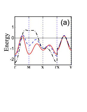
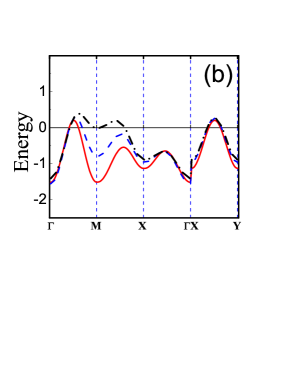
Figure 12: (Color online) Electron dispersion in the GMFA ${\varepsilon}_{2}({\bf k})$ for (a) $V=0$ and (b) $V=2$ at $U=8$ along the symmetry directions $\Gamma(0,0)\rightarrow M(\pi,\pi)\rightarrow X(\pi,0)\rightarrow\Gamma(0,0)$ and $X(\pi,0)\rightarrow Y(0,\pi)$ for $\delta=0.05\,$ (red solid line), $0.10$ (blue dashed line), and $0.25$ (black dash-dotted line). Fermi energy for hole doping is at $\omega=0$.

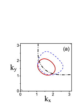
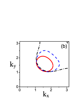
Figure 13: (Color online) Fermi surface for (a) $V=0$ and (b) $V=2$ at $U=8$ in the quarter of the BZ in the GMFA at hole doping $\delta=0.05$ (red solid line), $0.10$ (blue dashed line), and $0.25$ (black dash-dotted line).

.

To consider the self-energy effects in the electronic spectrum a strong coupling approximation (SCA) should be considered by a self-consistent solution of the system of equations for the normal GF (87) and the self-energy (88). In Ref. Plakida07 a detailed investigation of the normal state electronic spectrum for the conventional Hubbard model in SCA was performed. Here we present only the results of the electronic spectrum computation for the model (41) which are important for further studies of superconductivity in the model. The spectral function $\,A({\bf k},\omega)$ (90) along the symmetry directions is presented in Fig. 14 and the dispersion curves given by the maximum of this spectral function is displayed in Fig. 15 for the doping $\delta=0.10$. In Fig. 16 and Fig. 17 we plot the spectral function and the dispersion curves, respectively, for the doping $\delta=0.25$.

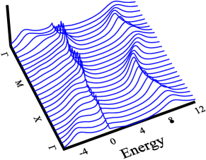
Figure 14: (Color online) Spectral function in the SCA along the symmetry directions $\Gamma(0,0)\rightarrow M(\pi,\pi)\rightarrow X(\pi,0)\rightarrow\Gamma(0,0)$ for hole concentration $\delta=0.10$.

Figure 15: (Color online) Electron dispersion curves in the SCA along the symmetry directions $\Gamma(0,0)\rightarrow M(\pi,\pi)\rightarrow X(\pi,0)\rightarrow\Gamma(0,0)$ for hole concentration $\delta=0.10$.

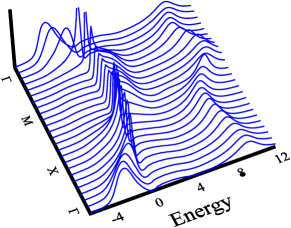
Figure 16: (Color online) Spectral function in the SCA along the symmetry directions for hole concentration $\delta=0.25$.

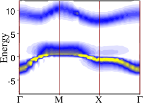
Figure 17: (Color online) Electron dispersion curves in the SCA along the symmetry directions for hole concentration $\delta=0.25$.

In comparison with the GMFA in Fig. 12, a rather flat energy dispersion is found with QP peaks at the FS. In general, strong increase of the dispersion and intensity of the QP peaks is observed in the overdoped region in comparison with the underdoped region. This is in agreement with our detailed studies of temperature and doping dependence of the self-energy (88) and spectral function (90) in Plakida07 which have proved strong influence of AF spin-correlations on the spectra.

Noticeable changes are observed for the FS in the SCA shown in Figs. 18 and 19 which are determined by the equation for the spectral density (90) at the Fermi energy, $\,A({\bf k},\omega=0)$. Whereas in GMFA at small doping the FS in Fig. 13 shows closed pockets, in SCA the FS reveals arc-type behavior detected in ARPES experiments where spectral function $\,A({\bf k},\omega=0)$ is measured (see, e.g., Ref. Shen05 ).

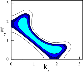
Figure 18: (Color online) $A({\bf k},\omega=0)$ on the FS at $\delta=0.05$ at $T=0.03t$ for $U=4t$.

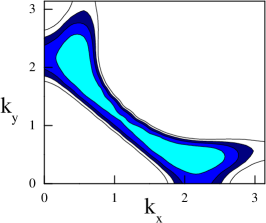
Figure 19: (Color online) $A({\bf k},\omega=0)$ on the FS $\delta=0.1$ at $T=0.03t$ for $U=4t$.

The arc-type behavior is related to formation of the pseudogap in the electronic spectrum induced by the AF spin-fluctuations as was found in the two-particle self-consistent approach (TPSC)  Vilk95 ; Tremblay06 or the model of short-range static spin (charge) fluctuations – the $\Sigma_{\bf k}$-model Sadovskii01 ; Sadovskii05 . To prove this, let us consider the static limit for the interaction (92) by taking into account only zero Matsubara frequency $i\omega_{\nu}=0$ which gives $i\omega_{m}=i\omega_{n}$ in (88). In the limit of the large AF correlation length $\xi\gg 1$ the static spin susceptibility $\chi_{s}({\bf q})$ in (95) shows a sharp peak close to the AF wave-vector ${\bf Q}=\pi(1,1)$ and can be expanded over the small wave-vector ${\bf p=q-Q}$:

$$\chi_{s}({\bf q})\simeq\,\frac{\chi_{Q}}{1+\xi^{2}\,{\bf p}^{2}}\simeq\frac{A}{\kappa^{2}+{\bf p}^{2}},$$ (101)

where we introduced $\kappa=\xi^{-1}$ and took into account that the constant (96) $\chi_{Q}\simeq A\,\xi^{2}$ with $\,A=({6\pi}/{\omega_{s}})[\ln(1+4\pi\,\xi^{2})]^{-1}$ for the square lattice. In this limit we get the following equation for the self-energy (88):

$${\Sigma}({\bf k},i\omega_{n})\simeq A\,|t({\bf k-Q})|^{2}\,\frac{T}{N}\sum_{\bf p}\,\frac{1}{{\kappa^{2}+p^{2}}}$$

$$\times[{G}_{1}({\bf k-Q-p},i\omega_{n})+{G}_{2}({\bf k-Q-p},i\omega_{n})].$$ (102)

Expanding the QP energy $\,\varepsilon_{1(2)}({\bf k-Q-p})\simeq\varepsilon_{1(2)}({\bf k-Q})-{\bf p\cdot v}_{1(2),\bf k-Q}\,$ we obtain for the GFs in (102) the following representation:

$${G}_{1(2)}({\bf k-Q-p},i\omega_{n})\simeq\{i\omega_{n}-{\varepsilon}_{1(2)}({\bf k-Q})$$ (103)

$$+ {\bf p\cdot v}_{1(2),\bf k-Q}-\Sigma({\bf k-Q},i\omega_{n})\}^{-1}.$$

The system of equations for the GFs (103) and the self-energy (102) is similar to those one derived in the TPSC approach Vilk95 ) and the $\Sigma_{\bf k}$-model Sadovskii01 ; Sadovskii05 ; Kuchinskii05 apart from the interaction function and the two-subband system of equations in our case. The coupling constant in Eq. (102) is determined by the hopping parameter $|t({\bf k-Q})|^{2}$, while in the TPSC and in the $\Sigma_{\bf k}$-model the coupling constant is related to the Coulomb scattering, $g^{2}=U^{2}(\langle n_{i\uparrow}n_{i\downarrow}\rangle/n^{2})\langle(n_{i\uparrow}-n_{i\downarrow})^{2}\rangle$. However, the values of these constants are close: the averaged over the BZ value $\langle\sqrt{|t({\bf k})|^{2}}\rangle_{{\bf k}}\sim 2t$ is comparable with the coupling constant used in Sadovskii05 . As in the TPSC theory, in the limit $\xi\rightarrow\infty$ the AF gap $\Delta_{AF}({\bf k})\propto|t({\bf k-Q})|^{2}$ in the QP spectra emerges in the subband located at the Fermi energy. This result readily follows from the self-consistent equations for the GF (87) with the self-energy (102) where in the right-had side the GF (103) is taken at ${\bf p}=0$. Thus, in our approach the pseudogap formation is mediated by the AF short-range order similar to TPSC theory and the model of short-range static spin fluctuations in the generalized DMFT Kuchinskii06 .

It is important to note that the superconducting $T_{c}$ in the gap equation (V.1) considerably depends on the quasiparticle weight determined by the renormalization parameter $Z({\bf q},\omega)$ in the self-energy (88). We estimate it at the Fermi energy

$$Z({\bf q}) = Z({\bf q},\omega=0)=1+\lambda({\bf q})$$ (104)

$$= 1-[\,d\,{\rm Re}\,\Sigma({\bf q},\omega)/{d\omega}]|_{\omega=0},$$

where we introduced the coupling constant $\lambda({\bf q})$. The doping dependence of $Z({\bf q})$ is shown in Fig. 20. It weakly depends on $\delta$ in the underdoped case for $\delta\lesssim 0.15$ but sharply decreases in the overdoped case for $\delta\gtrsim 0.25$. The temperature dependence of $Z({\bf q})$ presented in Fig. 21 is weak at temperatures lower than the characteristic energy of spin fluctuations $\omega_{s}\sim J$. The electron-phonon interaction gives a small contribution to the coupling constant as follows from the comparison of $Z({\bf q})$ induced by both spin-fluctuations and electron-phonon interaction contributions (red solid line) with the contribution caused only by spin-fluctuations (blue dashed line).

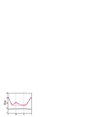
Figure 20: (Color online) Doping dependence of the renormalization parameter $Z({\bf q})$ along the symmetry directions $\Gamma(0,0)\rightarrow M(\pi,\pi)\rightarrow X(\pi,0)\rightarrow\Gamma(0,0)$ at $T\approx 140$ K for $\delta=0.05$ (red solid line), $\delta=0.10$ (blue dashed line), $\delta=0.15$ (red squares), $\delta=0.25$ (black dash-dotted line), and $\delta=0.35$ (black diamonds)

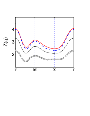
Figure 21: (Color online) Temperature dependence of the renormalization parameter $Z({\bf q})$ for $\delta=0.05$ at $T\approx 140$ K (red solid line), $T\approx 580$ K (black dash-dotted line), and $T\approx 1100$ K (black squares). Blue dashed line shows $Z({\bf q})$ for $\delta=0.05$ caused only by the spin-fluctuation contribution.

Thus, studies of the normal state electronic spectrum revealed a major role of AF correlations and self-energy effects in the renormalization of the spectrum. The latter show a noticeable reduction of the QP weight at low doping that strongly suppresses superconducting pairing as we demonstrate below.

V.3 Superconducting gap and $\bf T_{c}$

For a comparison of various contributions to the superconducting gap equation (V.1), we approximate the interaction (92) by its value close to the Fermi energy. As the result instead of the dynamical susceptibility (83), (84) the static susceptibility $\chi({\bf q})={\rm Re}\,\chi({\bf q},\Omega=0)$ appears in the gap equation. It brings us to the BCS-type equation for the gap function (V.1) at the Fermi energy $\varphi({\bf k})=\varphi({\bf k},\omega=0)$:

$$\varphi({\bf k})=\frac{1}{N}\sum_{{\bf q}}\,\frac{[1-b({\bf q})]^{2}\,\varphi({\bf q})}{[Z({\bf q})]^{2}\;2\widetilde{\varepsilon}({\bf q})}\tanh\frac{\widetilde{\varepsilon}({\bf q})}{2T_{c}}\big{\{}J({\bf k-q})$$

$$-V({\bf k-q})+\big{[}(1/4)|t({\bf q})|^{2}+|V({\bf k-q})|^{2}\big{]}\chi_{cf}({\bf k-q})$$

$$+|g({\bf k-q})|^{2}\,\chi_{ph}({\bf k-q})\,\theta(\omega_{0}-|\tilde{\varepsilon}({\bf q})|)$$

$$-|t({\bf q})|^{2}\;\chi_{sf}({\bf k-q})\theta(\omega_{s}-|\tilde{\varepsilon}({\bf q})|)\big{\}}\,,$$ (105)

where $\,\widetilde{\varepsilon}({\bf q})=\varepsilon_{2}({\bf q})/Z({\bf q})$ is the renormalized energy. Whereas for the exchange interaction and CI there are no retardation effects and the pairing occurs for all electrons in the two-particle subband, the electron-phonon interaction and spin-fluctuation contributions are restricted to the range of energies $\,\pm\omega_{0}\,$ and $\,\pm\omega_{s}$, respectively, near the FS as determined by the $\theta$-functions.

To estimate various contributions in the gap equation (105) we consider a model $d$-wave gap function, $\varphi({\bf k})=(\Delta/2)\,\eta({\bf k})$ where $\eta({\bf k})=(\cos k_{x}-\cos k_{y})$. Integrating Eq. (105) with the function $\eta({\bf k})$ over ${\bf k}$ we obtain the gap equation in the form:

$$1 = \frac{1}{N}\sum_{\bf q}\frac{[1-b({\bf q})]^{2}\,[\eta({\bf q})]^{2}}{[Z({\bf q})]^{2}\;2\widetilde{\varepsilon}({\bf q})}\tanh\frac{\widetilde{\varepsilon}({\bf q})}{2T_{c}}\big{\{}J-V$$ (106)

$$+ \widehat{V}_{cf}+(1/4)\,|t({\bf q})|^{2}\widehat{\chi}_{cf}+\widehat{V}_{ep}\,\theta(\omega_{0}-|\widetilde{\varepsilon}({\bf q})|)$$

$$- |t({\bf q})|^{2}\,\widehat{\chi}_{sf}\theta(\omega_{s}-|\widetilde{\varepsilon}({\bf q})|)\big{\}}.$$

In this equation only $l=2$ components of the static susceptibility and CI give contributions

$$\widehat{V}_{cf} = \frac{1}{N}\sum_{\bf k}|V({\bf k})|^{2}\,\chi_{cf}({\bf k})\,\cos k_{x},$$ (107)

$$\widehat{\chi}_{cf} = \frac{1}{N}\sum_{\bf k}\chi_{cf}({\bf k})\cos k_{x},$$ (108)

$$\widehat{V}_{ep} = \frac{g_{ep}}{N}\sum_{\bf k}S({\bf k})\cos k_{x},$$ (109)

$$\widehat{\chi}_{sf} = \frac{1}{N}\sum_{\bf k}\chi_{sf}({\bf k})\cos k_{x}\,.$$ (110)

The contribution from the charge fluctuations $\,\widehat{\chi}_{cf}\,$ (108) weakly depends on $U$ and $V$ and is very small: $\,\widehat{\chi}_{cf}\sim 10^{-3}\,(1/t)\,-10^{-2}\,(1/t)\,$ for hole concentrations $\delta=0.05-0.10$, respectively. For the averaged over the BZ vertex $\;\overline{|t({\bf q})|^{2}}=(1/N)\sum_{\bf q}|t({\bf q})|^{2}\simeq 4\,t^{2}$ the contribution induced by the kinematical interaction is equal to $\overline{|t({\bf q})|^{2}}\,\widehat{\chi}_{cf}\lesssim 0.04\,t\,$ and can be neglected. The charge fluctuation contribution $\,\widehat{V}_{cf}\,$ (107) from the intersite CI (100) for the hole concentration $\delta=0.05$ is also small, $\;\widehat{V}_{cf}\lesssim 5\cdot 10^{-2}\,t\;$ and $\,\widehat{V}_{cf}-V<0\,$ for all values of $\,U$ and $\,V$ and consequently, the $d$-wave pairing induced only by the charge fluctuations cannot occur.

The electron-phonon interaction contribution (109) for the electron-phonon interaction model (98) even for a strong electron-phonon interaction coupling $g_{ep}=5t$ is quite small for the $d$-wave pairing, $\,\widehat{V}_{ep}=2\,t\,(0.8\,t)\,$ for $\delta=0.05\,(0.25)$, as shown in Table 1. The electron-phonon interaction contribution to the $s$-wave pairing is given by the $l=0$ component $S_{0}=(1/N)\sum_{\bf q}\,S(q)=0.31\;(0.57)\,$ for $\xi_{ch}=2\;(10)$, respectively. The ratio of the $d$-wave $S_{d}$ and the $s$-wave $S_{0}$ components of the electron-phonon matrix elements is equal to $\,(S_{d}/S_{0})=0.43\;(0.60)$ for $\xi_{ch}=2\;(10)$, respectively. This shows that at small hole concentrations $\delta$ (large charge correlation lengths $\xi_{ch}=1/2\delta$) the electron-phonon interaction for the both components are comparable, while for the overdoped case the $d$-wave component $S_{d}$ becomes considerably smaller than the $s$-wave component in agreement with the results of Ref. Zeyher96 .

The spin-fluctuation contribution $\,\widehat{\chi}_{sf}\,$ (110) is calculated for the model $\chi_{sf}({\bf q})$ in Eq. (95). Since the spin susceptibility has a maximum at the AF wave vector ${\bf Q}=\pi\,(1,1)$ the integral over ${\bf k}$ in (110) results in the negative value for $\,\widehat{\chi}_{sf}\,$ which strongly depends on hole doping as shown in Table 1. Using the averaged over BZ vertex $\,\overline{|t({\bf q})|^{2}}\simeq 4\,t^{2}\,$ we can estimate an effective spin-fluctuation coupling constant as $\,g_{sf}\simeq-4\,t^{2}\,\widehat{\chi}_{sf}=5\,t-2\,t$ for $\delta=0.05-0.25$. Thus, the spin-fluctuation contribution to the pairing in Eq. (106) with the coupling constant $\,g_{sf}$ appears to be the largest.

First we calculate doping dependence of $T_{c}$ in the weak-coupling approximation (WCA) for $Z({\bf q})=1$ in Eq. (106) by taking into account the exchange interaction $J$, the Coulomb repulsion $V$, and the contributions from the self-energy $\,\widehat{V}_{ep}$, $\widehat{\chi}_{sf}$, and $\,\widehat{V}_{cf}$, neglecting the small contribution $\widehat{\chi}_{cf}$. Results of the calculation is shown in Fig. 22. The highest $T_{c}\approx 0.22\,t$ is found when all the contributions are taken into account. The spin-fluctuation pairing results in superconducting $T^{sf}_{c}\approx 0.1\,t$ much larger than $T^{ep}_{c}\approx 0.012t$ mediated by the electron-phonon interaction. For the ${\bf k}$-independent electron-phonon interaction $\,(S({\bf k})=1)\,$ there is no contribution to the $d$-wave pairing. The doping dependence of $T_{c}$ is qualitatively agree with experiments in cuprates but its value is an order of magnitude higher.

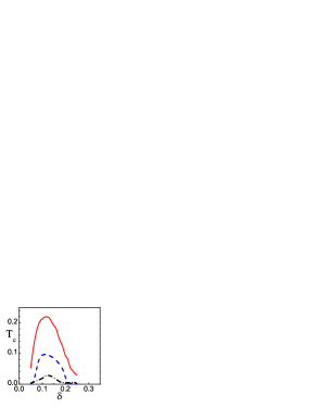
Figure 22: (Color online) $T_{c}(\delta)$ in the WCA induced by all interactions (red solid line) and only by the spin-fluctuation contribution (blue dashed line) or only by the electron-phonon interaction $\,\widehat{V}_{ep}\,$ (black dash-dotted line).

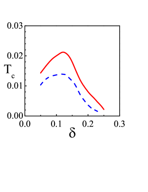
Figure 23: (Color online) $T_{c}(\delta)$ in the SCA induced by all interactions (red solid line) and only by the spin-fluctuation contribution (blue dashed line).

The high values for $T_{c}$ found in the WCA are explained by neglecting the reduction of the QP weight caused by the renormalization factor $Z({\bf q},\omega_{m})$ in the gap equation (V.1). In the SCA the gap equation (V.1) is convenient to write in the form:

$$\varphi({\bf k},\omega_{n})=\frac{T_{c}}{N}\sum_{\bf q}\,\sum_{m}\,\big{\{}J({\bf k-q})-V({\bf k-q})$$

$$+V_{ep}({\bf k-q},\omega_{n}-\omega_{m})-V_{sf}({\bf q,k-q},\omega_{n}-\omega_{m})\big{\}}$$

$$\times\frac{[1-b({\bf q})]^{2}\,\varphi({\bf q},\omega_{m})}{[\omega_{m}Z({\bf q},\omega_{m})]^{2}+[{\varepsilon}_{2}({\bf q})+X({\bf q},\omega_{m})]^{2}}\,.$$ (111)

For $V({\bf k-q})$ we take the nearest-neighbor CI (100). Since the charge fluctuations $\chi_{cf}({\bf k-q},\nu_{n})$ gives a much weaker contribution than the spin-fluctuations and electron-phonon interactions (see Table 1), we neglect them in the interaction function (92). Contributions induced by spin-fluctuations and the electron-phonon interaction are described by the functions

$$V_{sf}({\bf q,k-q},\omega_{\nu})=|t({\bf q})|^{2}\,\chi_{sf}({\bf k-q})F_{sf}(\omega_{\nu}),\quad$$ (112)

$$V_{ep}({\bf k-q},\omega_{\nu})=g_{ep}\,\frac{\omega_{0}^{2}}{\omega^{2}_{0}+\omega_{\nu}^{2}}\,S({\bf k-q}),$$ (113)

where the spectral function for spin fluctuations reads:

$$F_{sf}(\omega_{\nu})=\frac{1}{\pi}\int_{0}^{\infty}\frac{2xdx}{x^{2}+(\omega_{\nu}/\omega_{s})^{2}}\frac{\tanh(x\,\omega_{s}/2T)}{1+x^{2}}\,.$$ (114)

To calculate $T_{c}$ and to find out the energy- and ${\bf k}$-dependence of the gap $\,\varphi({\bf k},\omega)$, Eq. (111) was solved by a direct diagonalization in $({\bf k},\omega_{n})$-space. Since the largest contribution in Eq. (111) comes from energies close to the FS, we have used the renormalization parameters at the Fermi energy $Z({\bf q})$ (104) and $X({\bf q})$ instead of the energy dependent ones. The results for $T_{c}(\delta)$ is shown in Fig. 23. The highest $T_{c}\sim 0.021t\sim 100$ K is found when all the contributions are taken into account, though pairing induced only by spin-fluctuations also results in high $T^{sf}_{c}\sim 0.014t\sim 65$ K. The $d$-wave pairing induced only by the electron-phonon interaction is rather weak and does not displayed in Fig. 23. The value of $T_{c}$ is reduced by an order of magnitude in comparison with the WCA in Fig. 22 due to a suppression of the QP weight by the factor $[1/Z({\bf q})]^{2}$. The maximum value of $T_{c}$ is found at lower value of doping $\delta_{opt}\approx 0.12$ than in experiments, $\delta^{exp}_{opt}=0.16$.

The ${\bf k}$-dependence of the gap function $\varphi({\bf k},\omega\simeq 0)\,$ at doping $\delta=0.13$ for $\,(0\leq k_{x},\,k_{y}\leq 2\pi)$ is plotted in Fig. 24. The gap reveals a distinct $d$-wave symmetry with maximum values in the vicinity of the FS. As shown in Fig. 25, its angle dependence on the FS is close to the model $d$-wave dependence $\varphi_{d}(\theta)=\cos 2\theta$.

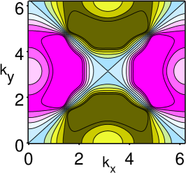
Figure 24: (Color online) 2D plot of the SC gap $\varphi({\bf k},\omega\simeq 0)$.

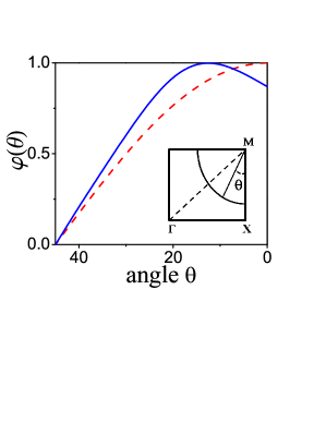
Figure 25: (Color online) Angle dependence of the SC gap $\varphi(\theta)$ on the FS (blue bold line) in comparison with the model $d$-wave dependence $\varphi_{d}(\theta)=\cos 2\theta$ (red dashed lines).

Energy dependence (in units of $\,t\,$) of the gap function $\varphi({\bf k},\omega)$, the real and imaginary parts, is presented in Fig. 26 at ${\bf k}\approx(0,\pi/2)$ and $\delta=0.13$. Since the gap function was obtained as a solution of the linear equation at $T=T_{c}$ the value of the gap is given in arbitrary units. The energy variation of the gap occurs in the region of $\omega\lesssim 0.4t$, of the order of the characteristic spin-fluctuation energy $\omega_{s}=J=0.4t$.

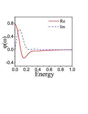
Figure 26: (Color online) Energy dependence of the real, Re $\varphi({\bf k},\omega)$, and imaginary, Im $\varphi({\bf k},\omega)$, parts of the SC gap in arbitrary units.

Dependence of the superconducting temperature $T_{c}$ on the intersite CI is shown in Fig. 27 for $\,V=0.0,\,0.5,\,1.0$, and $\,2\,$. Increasing of $V$ suppresses $T_{c}$ which becomes small only for high values of $V=2t-3t$ comparable with the spin-fluctuation coupling $\,g_{sf}$ and much larger than the exchange interaction $\,J=0.4t$. The maximum $T^{\rm max}_{c}$ at the optimal doping as a function of $U$ and $V$ is shown in Fig. 28. It is remarkable, that $T^{\rm max}_{c}$ only weakly depends on $\,U\,$ that supports the kinematical mechanism of pairing where the coupling constant $\,|t({\bf q})|^{2}\,$ does not depend on $U$. A weak increase of $T^{\rm max}_{c}$ with $U$ is explained by narrowing of the electronic band as seen in Figs. 12, 13 and corresponding increase of the density of state.

Figure 27: (Color online) $T_{c}(\delta)$ for $V=0.0$ (bold red line), $V=0.5$ (blue dashed line), $V=1.0$ (black dash-dotted line), and $V=2.0$ (green dotted line) for $U=8\,$.

Figure 28: (Color online) Maximum $T^{\rm max}_{c}$ at the optimal doping as a function of $U\,$ for $V=0.0$ (bold red line), $V=0.5$ (blue dashed line), and $V=1.0$ (black dash-dotted line).

In the current approach one can also consider the $s$-wave pairing. For the extended $s$-wave gap function, $\varphi_{s}({\bf k})=(\Delta/2)\,\eta_{s}({\bf k})$ where $\eta_{s}({\bf k})=(\cos k_{x}+\cos k_{y})$, a similar to (105) equation for $T_{c}$ can be derived. Solution of this equation reveals a finite and quite high $T_{c}$ as in Refs. Zaitsev04 ; Valkov11 where superconducting pairing in the Hubbard model was found to be robust in respect to the intersite Coulomb interaction $V$. However, the $s$-wave pairing violates the well known constraint of “no double occupancy” in strongly correlated systems. First, it was pointed out in Refs. Plakida89 ; Yushankhai91 for the $t$-$J$ model and then in Ref. Plakida14 for the Hubbard model. This constraint can be formulated in terms of a specific relation for the anomalous (pair) correlation function for the Hubbard operators. It is easy to verify that the product of two HOs for the singly occupied subband equals zero: $\,X_{i}^{0\sigma}X_{i}^{0\bar{\sigma}}=a_{i\sigma}(1-N_{i\bar{\sigma}})\,a_{i\bar{\sigma}}(1-N_{i\sigma})=0$. Therefore, the corresponding single-site pair correlation function should vanish:

$$F_{ii,\sigma}=\langle X_{i}^{0\sigma}X_{i}^{0\bar{\sigma}}\rangle=\frac{1}{N}\sum_{{\bf q}}\,\langle X_{\bf q}^{0\sigma}X_{-{\bf q}}^{0\bar{\sigma}}\rangle\equiv 0.$$ (115)

The symmetry of the Fourier-component of the pair correlation function $\,F_{\sigma}({\bf q})=\langle X_{\bf q}^{0\sigma}X_{-{\bf q}}^{0\bar{\sigma}}\rangle\,$ has the symmetry of the superconducting order parameter, i.e., the gap function. For instance, in the quasiparticle approximation we have

$$F_{\sigma}({\bf q})=\frac{\varphi(\bf q)}{[Z({\bf q})]^{2}\;2\widetilde{\varepsilon}({\bf q})}\tanh\frac{\widetilde{\varepsilon}({\bf q})}{2T_{c}}.$$ (116)

For the tetragonal lattice for the $d$-wave pairing $\,F_{\sigma}(q_{x},q_{y})=-F_{\sigma}(q_{y},q_{x})\,$ and the condition (115) after integration over $q_{x},q_{y}$ is fulfilled. For the $s$-wave pairing $\,F_{\sigma}(q_{x},q_{y})=F_{\sigma}(q_{y},q_{x})\,$ and the condition (115) is violated. The same condition holds for the pair correlation function for the second Hubbard subband, $\langle X_{i}^{\sigma 2}X_{i}^{\bar{\sigma}2}\rangle=0$. Therefore, the $s$-wave pairing in the both Hubbard subbands is prohibited in the limit of strong correlations.

To overcome the restriction (115) in Refs. Valkov03 it was proposed to consider the modified time-dependent pair correlation function:

$$\tilde{F}_{ii,\sigma}(t)=\int_{-\infty}^{+\infty}d\omega\,{\rm e}^{i\omega t}\,\tilde{J}_{ii,\sigma}(\omega),$$ (117)

where

$$\tilde{J}_{ii,\sigma}(\omega)={J}_{ii,\sigma}(\omega)-\delta(\omega)\;\int_{-\infty}^{+\infty}d\omega_{1}\,J_{ii,\sigma}(\omega_{1}).$$ (118)

The spectral density $\,{J}_{ii,\sigma}(\omega)\,$ determines the original correlation function

$${F}_{ii,\sigma}(t)=\langle{X_{i}^{0\sigma}}(t){X_{i}^{0\bar{\sigma}}}\rangle=\int_{-\infty}^{+\infty}d\omega\,{\rm e}^{i\omega t}\,{J}_{ii,\sigma}(\omega).$$ (119)

For the modified spectral density (118) the condition (115) is trivially satisfied for any spectral function $\,J_{ii,\sigma}(\omega)\,$ and the restriction on the $s$-wave pairing seems to be lifted. However, the spectral density (118) results in the nonergodic behavior Kubo57 of the pair correlation function (117):

$$C_{ii,\sigma}=\lim_{t\to\infty}\tilde{F}_{ii,\sigma}(t)=-\frac{1}{N}\sum_{{\bf q}}\,\langle X_{\bf q}^{0\sigma}X_{-{\bf q}}^{0\bar{\sigma}}\rangle,$$ (120)

where the conventional pair correlation function decays in the limit ${t\to\infty}$ due to finite life-time effects

$$\lim_{t\to\infty}{F}_{ii,\sigma}(t)=\int_{-\infty}^{+\infty}d\omega\,{\rm e}^{i\omega t}\,J_{ii,\sigma}(\omega)=0.$$ (121)

The nonergodic behavior of the modified pair correlation function (117) contradicts to the basic properties of physical systems and appears for some pathological models with local integrals of motion Suzuki71 ; Huber77 . In that case, the nonergodic constant can be found from $1/\omega$ poles of the anticommutator or causal Green functions, as described for the Hubbard model for spin or charge excitations in Refs. Mancini03 ; Avella07 contrary to the arbitrary definition (118). Therefore, the statement given in Refs. Valkov03 : “The inclusion of a singular contribution to the spectral intensity of the anomalous correlation function regains the sum rule and remove the unjustified forbidding of the $s$-symmetry order parameter in superconductors with strong correlations” cannot be accepted.

V.4 Isotope effect

The observation of the isotope effect (IE) in conventional superconductors, i.e., the dependence of $T_{\rm c}$ on the mass $M$ of the lattice ions, $T_{\rm c}\propto M^{-\alpha}$, with the isotope exponent $\alpha=-d\ln T_{\rm c}/d\ln M\simeq 0.5$ was a direct evidence of the electron-phonon pairing mechanism in these materials. In cuprate superconductors a weak isotope shift with $\alpha\leq 0.1$ was found at optimal doping. In the underdoped region isotope exponent increases and can be even larger than in conventional superconductors, $\alpha\sim 1\,$ (see, e.g., reviews  Zhao01 ; Khasanov04 ; Muller07 ). Small values of the isotope exponent at optimal doping suggests nonphononic, e.g., magnetic, mechanism of pairing. However, it is difficult to explain the IE on $T_{c}$ within the spin-fluctuation pairing mechanism. By taking into account the electron-phonon interaction within the extended Hubbard model (41) we can observe the IE in qualitative agreement with experiments.

To study the isotope effect on $T_{c}$ using the gap equation (106) we consider the mass-dependent phonon frequency $\omega_{0}$ in the $\theta$-function in (106), $\omega_{0}=\omega_{0}^{(0)}\sqrt{{M_{0}}/(M_{0}+\Delta M)}=\omega_{0}^{(0)}(1-\beta)$. For instance, for the oxygen isotope shift ¹⁶O $\rightarrow^{18}$O we have $\,\beta=0.057$. We neglect the polaronic effect for the $d$-wave electron-phonon coupling constant $\,g_{ep}({\bf q})=|g({\bf q})|^{2}\,\chi_{ph}({\bf q})\,$ assuming it to be mass-independent (for a discussion see Ref. Plakida11a ). The result for the isotope exponent found by numerical solution of the gap equation (106) is shown in Fig. 29 for two values of electron-phonon interaction $g_{ep}=5\,t$ and $g_{ep}=2.5\,t\,$ in Eq. (109) for $Z({\bf q})=5$. The doping dependence of the exponent agrees with experiments, it is quite small, $\,\alpha=0.09-0.18\,$, at doping close to the optimal, while drastically increases in the underdoped case, $\,\alpha=0.38-0.68\,$ at $\delta=0.1$ for $g_{ep}=2.5\,t-5\,t\,$, respectively.

Figure 29: (Color online) Isotope exponent $\alpha(\delta)$ for $g_{ep}=5\,t$ (red solid line) and $g_{ep}=2.5\,t$ (blue dashed line).

Similar results were obtained in Ref. Shneyder09 for the $t$-$J$ model with the electron-phonon interaction.

V.5 Comparison with previous theoretical studies

In studies of superconductivity in the framework of the conventional Hubbard model in the limit of strong correlations the MFA has been often used (see, e.g., Refs. Beenen95 ; Avella97a ; Stanescu00 ; Mancini03 ; Avella07 ; Avella07b ). As was shown in Sec IV.2, superconducting pairing in MFA is induced by the exchange interaction $\,J_{ij}={4t^{2}}/{U}$ (see Eq. (77)). The exchange interaction vanishes in the limit $\,U\to\infty\,$, a feature which explains the disappearance of the pairing at large $U$ observed in Refs. Beenen95 ; Avella97a ; Stanescu00 . To obtain nonzero pairing in the limit $U\gg t$ the self-energy contribution induced by the kinematical interaction should be taken into account which does not depend on $U$ as shown in Fig. 28.

In the limit of strong correlations various numerical methods were extensively used. Here we refer to numerical simulations for finite clusters (see reviews Dagotto94 ; Bulut02 ; Scalapino07 ; Senechal12r ), the DMFT (see reviews Georges96 ; Kotliar06 ), the dynamical cluster approximation (DCA) Maier05 ; Maier06 and the cluster DMFT (see, e.g., Refs. Haule07 ; Kancharla08 ). More accurate results have been obtained within the DCA and cluster DMFT methods where short-range AF correlations are partially taken into account. Extensive numerical studies for finite clusters have revealed a tendency to the $d$-wave pairing in the Hubbard model, though a delicate balance between superconductivity and other instabilities (AF, spin-density wave, charge-density wave, etc.) was found (see, e.g., Refs. Bulut02 ; Scalapino07 ; Maier05 ; Maier06 ; Kancharla08 ). In Ref. Macridin09 ), using the DCA with the quantum Monte Carlo method, the superconducting $d$-wave pairing and the isotope effect similar to observed in cuprates were found for the Hubbard-Holstein model. However, in several publications an appearance of the long-range superconducting order has not been confirmed (see, e.g., Ref. Aimi07 ).

As discussed in Sec. V.3, the intersite Coulomb repulsion $V$ is detrimental for pairing induced by the on-site CI $U$ in the Hubbard model or higher-order contributions from $V$ in the weak correlation limit. Here we would like to comment on several studies of this problem in the strong correlation limit and to compare them with our analytical results for the $d$-wave pairing. Following the original idea of Anderson Anderson87 , it is commonly believed that the exchange interaction $\,J=4t^{2}/U\,$ induced by the interband hopping in the Hubbard model plays the major role in the $d$-wave superconducting pairing. Since the excitation energy of electrons in the interband hopping $\,U\,$ is much larger than their intraband kinetic energy $\,W\,$ the exchange pairing has no retardation effects contrary to the electron-phonon pairing where large Bogoliubov-Tolmachev logarithm Bogoliubov58 diminishes the Coulomb repulsion $V\rightarrow V/[1+\rho_{c}\,\ln(\mu/\omega_{ph})]$ where $\rho_{c}=N(0)\,V$ and $\omega_{ph}$ is the phonon energy. Consequently, without the retardation effects the Coulomb repulsion $V$ should destroy the exchange pairing for $\,V>J\,$.

Our conclusion concerning importance of the kinematical mechanism of pairing is supported by the studies in Ref. Plekhanov03 . Using the variational Monte Carlo technique the superconducting $d$-wave gap was observed for the extended Hubbard model with a weak exchange interaction $J=0.2\,t$ and a repulsion $V\leq 3\,t$ in a broad range of $\,0\leq U\leq 32$. It was found that the gap decreases with increasing $V$ at all $U$ and can be suppressed for $V>J$ for small $\,U$. But for large $\,U\gtrsim U_{c}\sim 6\,t\,$ the gap becomes robust and exists up to large values of $V\sim 10\,J=2\,t$ which was explained by effective enhancement of $J$. At the same time, the gap does not show notable variation with $U$ for large $U=10-30$ though it should depend on the conventional exchange interaction in the Hubbard model $J=4t^{2}/U$ (or $J=4t^{2}/(U-V)$). We can suggest another explanation of these results by pointing out that at large $U\gtrsim U_{c}\,$ concomitant decrease of the bandwidth (as shown in Fig. 3 b in Ref. Plekhanov03 ) results in the splitting of the Hubbard band into the upper and lower subbands and the emerging kinematical interaction induces the $d$-wave pairing in one Hubbard subband. In that case the second subband for large $U$ gives a small contribution which results in $U$-independent pairing as shown in Fig. 28. It can be suppressed by the repulsion $V$ only larger than the kinematical interaction, $V\gtrsim 4t$.

In Ref. Raghu12a the extended Hubbard model is considered in the weak or intermediate correlation limits as in Ref. Raghu12 and in the strong correlation limit within the slave-boson representation in the MFA. In the strong correlation limit a small value of $V=J$ suppresses the $d$-wave superconducting gap. The kinetic energy term described by the projected electron operators, $t\,\hat{c}_{i\sigma}^{\dagger}\hat{c}_{j\sigma}=t\,{c}_{i\sigma}^{\dagger}(1-n_{i-\sigma}){c}_{j\sigma}(1-n_{j-\sigma})\equiv t\,X_{i}^{\sigma 0}X_{j}^{0\sigma}$, was approximated by the conventional fermion (spinon) operators, $t\,\delta\,f_{i\sigma}^{\dagger}f_{j\sigma}$ where the slave-boson contribution in the MFA was described by the hole concentration $\delta$. In this approximation the most important contribution from the kinematical interaction given by $\widehat{\chi}_{sf}$ (110) in Eq. (106) was lost in the resulting BCS-type gap equation (13) in Ref. Raghu12a . Thus, the slave-boson theory treated in MFA fails to describe superconducting pairing in the limit of strong correlations.

In Refs. Feng03 ; Feng04 ; Feng06 the slave-boson representation was considered beyond the MFA within the extended $t$-$J$ model. A kinetic-energy driven mechanism of superconductivity in the effective fermion-spin theory was proposed where the pairing of fermions is induced by spin excitations described by slave bosons. A special procedure of the charge-spin separation and then the charge-spin recombination have been used in calculation of the electronic GFs. Similar to our kinematic spin-fluctuation pairing theory, the Eliashberg-type system of equations was obtain where the coupling constant is given by the hopping parameter. However, as in the conventional slave-boson theory the local constraint of no double occupancy cannot be treated rigorously contrary to the HO technique used in our theory. Nevertheless, this approach yields many results such as doping dependence of $T_{c}$, the normal state pseudogap, electromagnetic response, charge transport which are in a broad agreement with experiments in cuprates  Feng15 .

VI Conclusion

In the present review we present the microscopic theory of spin excitations and superconductivity for strongly correlated electronic systems as cuprates. Studies of the spin excitations in the normal state have shown a crossover from well-defined spin-wave-like excitations at low doping and temperatures to relaxation-type spin-fluctuation excitations (AF paramagnon) with increasing hole doping. This results agree with inelastic neutron-scattering experiments, RIXS and numerical simulations for finite clusters. We propose a new explanation for the magnetic RM observed in superconducting state. As was shown in Sec. III.4, a weak damping of spin excitations close to the AF wave vector ${\bf Q}$ is the reason for appearance of the RM. The weak damping of the RM is explained by a contribution from spin excitations to the decay process besides a particle-hole pair usually considered in the spin-1 exciton scenario. In this case the temperature independent RM at $E_{\rm r}$ appears since the damping essentially depends on the gap $\widetilde{\omega}_{\bf Q}\simeq E_{\rm r}$ in the spin-excitation spectrum and opening of the superconducting gap $2\Delta(T)$ below $T_{\rm c}$ is less important.

The theory of superconducting pairing was developed within the extended Hubbard model (41) in the limit of strong electron correlations. Using the Mori-type projection technique we obtained a self-consistent system of equations for the normal and anomalous (pair) GFs and for the self-energy calculated in the SCBA. From our study we can draw the following conclusion concerning the mechanism of pairing in the extended Hubbard model. Solution of the gap equation shows that for the $d$-wave pairing relevant contributions come from the $l=2$ angular momentum component of interactions. This results in a considerable reduction of the intersite Coulomb repulsion and electron-phonon interaction. In particular, a momentum independent electron-phonon interaction give no contribution to the $d$-wave pairing. At the same time, a strong local electron-phonon interaction may induce a noticeable polaronic effect observed in the magnetic penetration depth Khasanov04 . Thus we conclude that the electron-phonon interaction plays a secondary role in achieving high-$T_{c}$ though it should be taken into account to explain the weak isotope effect on $T_{c}$. The largest contribution to the $d$-wave pairing comes from the electron coupling to spin fluctuations induced by the strong kinematical interaction $|t({\bf q})|$ which brings about the superconductivity with high $T_{c}$ observed in cuprates.

It is important to point out that the kinematical interaction induced by the kinetic energy of electrons moving in the Hubbard subband is responsible both for the damping of spin excitations at finite doping and the spin-fluctuation superconducting pairing. The kinematical interaction is characteristic for systems with strong electron correlations which is absent in the fermionic models. Therefore, we believe that the spin-fluctuation magnetic mechanism of superconducting pairing in the Hubbard model in the limit of strong correlations is a relevant mechanism of high-temperature superconductivity in the copper-oxide materials.

Acknowledgments

The author thanks S. Adam, G. Adam, D. Ihle, V. Oudovenko, and A. Vladimirov for the fruitful collaboration. The author is grateful to the MPIPKS, Dresden, for the hospitality during his stay at the Institute, where a part of these investigations has been done. The work was supported by the Heisenberg–Landau Program of JINR.

References

- (1) J. G. Bednorz and K. A. Müller, Z. Phys. B. 64 (1986) 189.
- (2) Handbook of High-Temperature Superconductivity. Theory and Experiment, J.R. Schrieffer and J.S. Brooks (Eds.), Springer-Verlag, New York, 2007.
- (3) N. M. Plakida, High-Temperature Cuprate Superconductors, Springer-Verlag, Berlin, 2010, 570 pp.
- (4) M. L. Kulić, in: A. Avella, F. Mancini (Eds.), Lectures on Physics of Highly Correlated Electronic Systems VIII, AIP Conf. Proc., Vol. 715, Melville, New York, 2004, p. 75.
- (5) E.G. Maksimov, M.L. Kulić, and O. V. Dolgov, Adv. in Cond. Mat. Phys., 2010, Article ID 423725 (DOI: 10.1155/2010/423725).
- (6) D.J. Scalapino, Phys. Reports 250 (1995) 329.
- (7) Rev. Mod. Phys. 84 (2012) 1383–1417.
- (8) P. Monthoux and D. Pines, Phys. Rev. B 49 (1994) 4261.
- (9) T. Moriya and K. Ueda, Adv. in Physics 49 (2000) 555; Rep. Prog. Phys. 66 (2003) 1299.
- (10) A. V. Chubukov, D. Pines, and J. Schmalian, in: K. H. Bennemann, J. B. Ketterson (Eds.), The Physics of Conventional and Unconventional Superconductors, Springer-Verlag, Berlin, 2004, Vol. I, p. 495; Ar. Abanov, A.V. Chubukov, and J. Schmalian, Advances in Phys. 52 (2003) 119.
- (11) Ar. Abanov, A.V. Chubukov, and M.R. Norman, Phys. Rev. B 78 (2008) 220507(R).
- (12) Ph. Bourges, From magnons to the resonance peak: Spin dynamics in high- superconducting cuprates by inelastic neutron scattering, in: J. Bok, G. Deutscher, D. Pavuna, S.A. Wolf (Eds.), The Gap Symmetry and Fluctuations in High Temperature Superconductors, Vol. 371 in NATO ASI series, Physics, Plenum Press, 1998, p. 349-371.
- (13) M. Le Tacon, G. Ghiringhelli, J. Chaloupka, M. Moretti Sala, V. Hinkov, M.W. Haverkort, M. Minola, M. Bakr, K. J. Zhou, S. Blanco-Canosa, C. Monney, Y. T. Song, G. L. Sun, C. T. Lin, G. M. De Luca, M. Salluzzo, G. Khaliullin, T. Schmitt, L. Braicovich, and B. Keimer, Nature Phys. 7 (2011) 725.
- (14) M. Le Tacon, M. Minola, D. C. Peets, M. Moretti Sala, S. Blanco-Canosa, V. Hinkov, R. Liang, D. A. Bonn, W. N. Hardy, C. T. Lin, T. Schmitt, L. Braicovich, G. Ghiringhelli, and B. Keimer, Phys. Rev. B 88 (2013) 020501(R).
- (15) M. P. M. Dean, G. Dellea, R. S. Springell, F. Yakhou-Harris, K. Kummer, N. B. Brookes, X. Liu, Y-J. Sun, J. Strle, T. Schmitt, L. Braicovich, G. Ghiringhell, I. Božović and J. P. Hill, Nature Mat. 12 (2013) 1019.
- (16) M. P. M. Dean, A. J. A. James, A. C. Walters, V. Bisogni, I. Jarrige, M. Hücker, E. Giannini, M. Fujita, J. Pelliciari, Y. B. Huang, R. M. Konik, T. Schmitt and J. P. Hill, Phys. Rev. 90 (2014) 220506(R).
- (17) M. Minola, G. Dellea, H. Gretarsson, Y. Y. Peng, Y. Lu, J. Porras, T. Loew, F. Yakhou, N.B. Brookes, Y.B. Huang, J. Pelliciari, T. Schmitt, G. Ghiringhelli, B. Keimer, L. Braicovich, and M. Le Tacon, Phys. Rev. Lett. 114 (2015) 217003.
- (18) A.A. Kordyuk, V.B. Zabolotnyy, D.V. Evtushinsky, D.S. Inosov, T.K. Kim, B. Büchner, and S.V. Borisenko, Eur. Phys. J. 188 (2010) 153.
- (19) A.A. Vladimirov, D. Ihle, and N.M. Plakida, Phys. Rev. B 85 (2012) 224536.
- (20) G.-M. Zhao, H. Keller, and K. Conder, J. Phys.: Condens. Matter 13 (2001) R569.
- (21) R. Khasanov, A. Shengelaya, E. Morenzoni, K. Conder, I.M. Savic̀, and H. Keller, J. Phys.: Condens. Matter 16 (2004) S4439.
- (22) K.A. Müller, in: J.R. Schrieffer and J.S. Brooks (Eds.), Handbook of High-Temperature Superconductivity. Theory and Experiment, Springer-Verlag, New York, 2007, pp. 1–18.
- (23) P. Fulde, Electronic correlations in molecules and solids, third ed., Springer Verlag, Berlin, 1995, 480 pp.
- (24) A.A. Vladimirov, D. Ihle, and N. M. Plakida, Phys. Rev. B 80 (2009) 104425.
- (25) A.A. Vladimirov, D. Ihle, and N. M. Plakida, Phys. Rev. B 83 (2011) 024411.
- (26) N.M.Plakida, Fizika Nizkikh Temperatur (J. Low Temp. Phys.) 32 (2006) 483.
- (27) N.M. Plakida V.S. Oudovenko, JETP 104 (2007) 230.
- (28) N. M. Plakida and V. S. Oudovenko, Eur. Phys. J. B 86 (2013) 115.
- (29) N. M. Plakida and V. S. Oudovenko, Zh. Exp.Theor. Fyz., 146 (2014) 631 [JETP 119 (2014) 554].
- (30) J. Hubbard, Proc. Roy. Soc. (London) A, 276 (1963) 238.
- (31) J. Hubbard, Proc. Roy. Soc. A 285 (1965) 542.
- (32) F. Dyson, Phys. Rev. 102 (1956) 1217.
- (33) Yu. A. Izyumov, Usp. Fiz. Nauk 167 (1997) 465, [Phys.- Usp. 40 (1997) 445].
- (34) Yu. A. Izyumov and B. M. Letfulov, J. Phys.: Condens. Matter, 2 (1990) 8905; Yu. A. Izyumov and J. A. Hedersen, Int. J. Mod. Phys. B 8 (1994) 1877.
- (35) E. Dagotto, Rev. Mod. Phys 66 (1994) 763.
- (36) J. Jaklič and P. Prelovšek, Adv. in Phys. 49 (2000) 1.
- (37) R. Eder, Y Ohta, and S. Maekawa, Phys. Rev. Lett. 74 (1995) 5124.
- (38) D.N. Zubarev, Usp. Fiz. Nauk, 71, (1960) 71; [Sov. Phys. Usp. 3, (1960) 320]; Nonequilibrium Statical Thermodynamics, Consultant Bureau, New-York, 1974.
- (39) N.M.Plakida, Phys. Lett. A 43 (1973) 481.
- (40) Yu.A. Tserkovnikov, Theor. Math. Phys. 49, (1981) 993; Theor. Math. Phys. 52 (1982) 712.
- (41) N. M. Plakida, Projection operator method, in: A. Avella, F. Mancini (Eds.), Theoretical Methods for Strongly Correlated Systems, Springer Series in Solid-State Sciences Vol. 171, Springer, Heidelberg, 2011, Chap. 6, pp. 173–202.
- (42) S. Winterfeldt and D. Ihle. Phys. Rev. B 58 (1998) 9402.
- (43) S. Winterfeldt and D. Ihle, Phys. Rev. B 56 (1997) 5535.
- (44) S. Winterfeldt and D. Ihle. Phys. Rev. B 59 (1999) 6010.
- (45) I. Sega, P. Prelovšek, and J. Bonča, Phys. Rev. B 68 (2003) 054524.
- (46) P. Prelovšek, I. Sega, and J. Bonča, Phys. Rev. Lett. 92 (2004) 027002.
- (47) A. Sherman and M. Schreiber, Eur. Phys. J. B 32 (2003) 203.
- (48) A. Sherman, Phys. Rev. B 70 (2004) 184512.
- (49) A. Sherman and M. Schreiber, Fizika Nizkikh Temperatur (J. Low Temp. Phys.) 32 (2006) 499.
- (50) A. Sherman and M. Schreiber, Phys. Rev. B 68 (2003) 094519.
- (51) I. Sega and P. Prelovšek Phys. Rev. B 73 (2006) 092516.
- (52) P. Prelovšek and I. Sega, Phys. Rev. B 74 214501 (2006).
- (53) A.A. Vladimirov, D. Ihle, and N. M. Plakida, Theor. Math. Phys. 145 (2005) 1575.
- (54) H. Mori, Prog. Theor. Phys. 34 (1965) 399.
- (55) H. Shimahara and S. Takada, J. Phys. Soc. Jpn. 60 (1991) 2394.
- (56) E. Manousakis, Rev. Mod. Phys. 63 (1991) 1.
- (57) J. Bonča, P. Prelovšek, and I. Sega, Europhys. Lett. 10 (1989) 87.
- (58) U.-J. Wiese and H.-P. Ying, Z. Phys. B 93 (1994) 147.
- (59) M. Vojta and K. Becker, Phys. Rev. B 54 (1996) 15483.
- (60) M.A. Kastner, R.J. Birgeneau, G. Shirane, and Y. Endoh, Rev. Mod. Phys. 40 (1998) 897.
- (61) J. Jaklič and P. Prelovšek, Phys. Rev. Lett. 77 (1996) 892.
- (62) M. Makivić and M. Jarrell, Phys. Rev. Lett. 68 (1992) 1770.
- (63) J. Rossat-Mignod, L. P. Regnault, C. Vettier, P. Bourges, P. Burlet, J. Bossy, J. Y. Henry, and G. Lapertot, Physica C, 185–189 (1991) 86.
- (64) Y. Sidis, S. Pailhès, B. Keimer, Ph. Bourges, C. Ulrich, and L.P. Regnault, phys. stat. sol. (b) 241 (2004) 1204.
- (65) H. He, P. Bourges, Y. Sidis, C. Ulrich, L. P. Regnault, S. Pailhès, N. S. Berzigiarova, N. N. Kolesnikov, and B. Keimer, Science 295 (2002) 1045.
- (66) G. Yu, Y. Li, E. M. Motoyama, X. Zhao, N. Barisic, Y. Cho, P. Bourges, K. Hradil, R. A. Mole, and M. Greven, Phys. Rev. B 81 (2010) 064518.
- (67) S. D. Wilson, P. Dai1, S. Li, S. Chi, H. J. Kang, and J. W. Lynn, Nature 442, (2006) 59.
- (68) C. Stock, W.J.L. Buyers, R. Liang, D. Peets, Z. Tun, D. Bonn, W.N. Hardy, and R.J. Birgeneau, Phys. Rev. B 69, (2004) 014502.
- (69) C. Stock, W.J.L. Buyers, R.A. Cowley, P.S. Clegg, R. Coldea, C.D. Frost, R. Liang, D. Peets, D. Bonn, W.N. Hardy, and R.J. Birgeneau, Phys. Rev. B 71 (2005) 024522.
- (70) Y. Sidis, S. Pailhès, V. Hinkov, B. Fauqué, C. Ulrich, L. Capogna, A. Ivanov, L.-P. Regnault, B. Keimer, and P. Bourges, C. R. Physique, 8 (2007) 745.
- (71) M. Eschrig, Adv. Phys. 55, (2006) 47.
- (72) M. R. Norman, Phys. Rev. B 61 (2000) 14751.
- (73) D. Manske, I. Eremin, and K. H. Bennemann, Phys. Rev. B 63 (2001) 054517.
- (74) I. Eremin, D.K. Morr, A.V. Chubukov, K. Bennemann, and M.R. Norman, Phys. Rev. Lett. 94 (2005) 147001.
- (75) F. Onufrieva and P. Pfeuty, Phys. Rev. B 65 (2002) 054515.
- (76) Gh. Adam and S. Adam, J. Phys. A: Math. Theor. 40 (2007) 11205.
- (77) P. W. Anderson, Science 235, 1196 (1987); P. W. Anderson, The theory of superconductivity in the high- cuprates, Princeton University Press, Princeton, 1997.
- (78) N.M. Plakida, L. Anton, S. Adam, and Gh. Adam, Zh. Exp.Theor. Fyz. 124, (2003) 367 [JETP 97, (2003) 331].
- (79) R.O. Zaitsev, and V.A. Ivanov, JETP Lett. 46 S116 (1987), Soviet Phys. Solid State 29 (1987) 2554, Ibid. 29 (1987) 3111, Int. J. Mod. Phys. B 5 (1988) 153.
- (80) Yu.A. Izyumov and B.M. Letfulov, J. Phys.: Condens. Matter 3 (1991) 5373.
- (81) N.M. Plakida, Physica C 282–287 (1997) 1737.
- (82) A.B. Migdal, Zh. Eksp. Teor. Fiz. 34 1438 (1956), [Soviet Phys. JETP 7 (1958) 996].
- (83) G.M. Eliashberg, Zh. Eksp. Teor. Fiz. 38 (1960) 966; ibid 39, 1437 (1960) [Soviet Phys. JETP 11 (1960) 696; ibid 12 (1960) 1000].
- (84) J. Jaklič and P. Prelovśek, Phys. Rev. Lett. 74 (1995) 3411; ibid. 75 (1995) 1340.
- (85) A.I. Lichtenstein. and M.L. Kulić, Physica C 245 (1995) 186.
- (86) R. Zeyher and M. L. Kulić, Phys. Rev. B 53 (1996) 2850.
- (87) L.F. Feiner, J.H. Jefferson, and R. Raimondi, Phys. Rev. B 53 (1996) 8751.
- (88) E. Plekhanov, S. Sorella, and M. Fabrizio, Phys. Rev. Lett. 90 (2003) 187004.
- (89) A.A. Kordyuk, S.V. Borisenko, A. Koitzsch, J. Fink, M. Knupfer, and H. Berger, Phys. Rev. B 71 (2005) 214513.
- (90) A. Georges, G. Kotliar, W. Krauth, and M. Rozenberg, Rev. Mod. Phys. 68 (1996) 13.
- (91) G. Kotliar, S. Y. Savrasov, K. Haule, V.S. Oudovenko, O. Parcollet, and C.A. Marianetti, Rev. Mod. Phys. 78 (2006) 865.
- (92) K. Haule and G. Kotliar, Phys. Rev. B 76 (2007) 104509.
- (93) K.M. Shen, F. Ronning, D. H. Lu, F. Baumberger, N. J. C. Ingle, W. S. Lee, W. Meevasana, Y. Kohsaka, M. Azuma, M. Takano, H. Takagi, and Z.-X. Shen, Science 307 (2005) 901.
- (94) Y. Vilk and A.-M. Tremblay, J. Phys. Chem. Solids (UK) 56 (1995) 1769.
- (95) A-M.S. Tremblay, B. Kyung and D. Sénéchal, Fizika Nizkikh Temperatur (J. Low Temp. Phys.) 32 (2006) 561.
- (96) M.V. Sadovskii, Usp. Phys. Nauk 171 (2001) 539. [Physics-Uspekhi 44 (2001) 515].
- (97) M.V. Sadovskii, I.A. Nekrasov, E.Z. Kuchinskii, Th. Pruschke, and V.I. Anisimov, Phys. Rev. B 72 (2005) 155105.
- (98) E.Z. Kuchinskii, I.A. Nekrasov, M.V. Sadovskii, Pis’ma v Zh. Exp. Teor. Fiz. 82 217 (2005). [JETP Letters 82 (2005) 198].
- (99) E.Z. Kuchinskii, I.A. Nekrasov, M.V. Sadovskii, Fizika Nizkikh Temperatur (J. Low Temp. Phys.) 32 (2006) 528.
- (100) R. O. Zaitsev, J. Exp. Theor. Phys. 98 (2004) 780.
- (101) V. V. Val’kov and M. M. Korovushkin, J. Exp. Theor. Phys. 112 (2011) 108.
- (102) N.M. Plakida, V.Yu. Yushankhai, and I.V. Stasyuk, Physica C 160 (1989) 80.
- (103) V.Yu. Yushankhai, N.M. Plakida, and P. Kalinay, Physica C 174 (1991) 401.
- (104) V. V. Val’kov, D. M. Dzebisashvili, and A.S. Kravtsov, JETP Letters 77 (2003) 505; Doklady USSR Acad. of Science 393 (2003) 1.
- (105) R. Kubo, J. Phys. Soc. Jpn. 12 (1957) 570.
- (106) M. Suzuki, Physica 51 (1971) 277.
- (107) D.L. Huber, Physica A, 87 A (1977) 199.
- (108) F. Mancini, A. Avella, Eur. Phys. J. B 36 (2003) 37.
- (109) A. Avella, F. Mancini, J. Phys.: Condens. Matter 19 (2007) 255209.
- (110) N. M. Plakida, Phys. Scr. 83 (2011) 038303.
- (111) E.I. Shneyder and S.G. Ovchinnikov, Zh. Eksp. Teor. Fiz. 136 (2009) 1177.
- (112) J. Beenen and D.M. Edwards, Phys. Rev. B 52 (1995) 13636.
- (113) A. Avella, F. Mancini, D. Villani, and H. Matsumoto, Physica C 282–287 (1997) 1757; T. Di Matteo, F. Mancini, H. Matsumoto, and V. S. Oudovenko, Physica B, 230–232 (1997) 915.
- (114) T. D. Stanescu, I. Martin, and Ph. Phillips, Phys. Rev. B 62 (2000) 4300.
- (115) A. Avella and F. Mancini, Phys. Rev. B 75 (2007) 134518.
- (116) N. Bulut, Advances in Physics 51 (2002) 1587.
- (117) D.J. Scalapino, Numerical studies of the 2D Hubbard model, in: J.R. Schrieffer and J.S. Brooks (Eds.), Handbook of High-Temperature Superconductivity. Theory and Experiment, Springer-Verlag, New York, 2007, pp. 495–526.
- (118) D. Sénéchal, Cluster dynamical mean field theory, in: A. Avella, F. Mancini (Eds.), Theoretical methods for Strongly Correlated Systems, Springer Series in Solid-State Sciences, Vol. 171, Springer- Verlag, Berlin, 2012, Chap. 11.
- (119) Th. Maier, M. Jarrel, Th. Pruschke, and M.H. Hettler, Rev. Mod. Phys. 77 (2005) 1027.
- (120) Th. A. Maier, M. Jarrell, and D.J. Scalapino, Phys. Rev. Lett. 96 (2006) 047005; ibid, Phys. Rev. B 74 (2006) 094513.
- (121) S. S. Kancharla, B. Kyung, D. Sénéchal, M. Civelli, M. Capone, G. Kotliar, and A.-M. S. Tremblay, Phys. Rev. B 77 (2008) 184516.
- (122) A. Macridin and M. Jarrell, Phys. Rev. B 79 (2009) 104517.
- (123) T. Aimi and M. Imada, J. Phys. Soc. Jpn. 76 (2007) 13708.
- (124) N. N. Bogoliubov, V. V. Tolmachev, D. V. Shirkov, New method in the theory of superconductivity, Publ. Dept. USSR Acad. of Science, Moscow, 1958; Consultants Bureau, Chapman and Hall, New York - London, 1959, Vol. YII.
- (125) S. Raghu, R. Thomale, and T. H. Geballe, Phys. Rev. B 86 (2012) 094506.
- (126) S. Raghu, E. Berg, A. V. Chubukov, and S. A. Kivelson Phys. Rev. B 85 (2012) 024516.
- (127) S. Feng, Phys. Rev. B 68 (2003) 184501.
- (128) S. Feng, T. Ma and H. Guo, Physica C 436 (2006) 14; T. Ma, H. Guo and S. Feng, Mod. Phys. Lett. B 18 (2004) 895.
- (129) S. Feng and T. Ma, Phys. Lett. A 350 (2006) 138.
- (130) S. Feng, Yu Lan, H. Zhao, L. Kuang, L. Qin and X. Ma, Int. J. Modern Phys. B 29 (2015) 1530009.