Interpolation-Based GR(1) Assumptions Refinement

Abstract

This paper considers the problem of assumptions refinement in the context of unrealizable specifications for reactive systems. We propose a new counterstrategy-guided synthesis approach for GR(1) specifications based on Craig’s interpolants. Our interpolation-based method identifies causes for unrealizability and computes assumptions that directly target unrealizable cores, without the need for user input. Thereby, we discuss how this property reduces the maximum number of steps needed to converge to realizability compared with other techniques. We describe properties of interpolants that yield helpful GR(1) assumptions and prove the soundness of the results. Finally, we demonstrate that our approach yields weaker assumptions than baseline techniques, and finds solutions in case studies that are unsolvable via existing techniques.

1 Introduction

Constructing formal specifications of systems that capture user requirements precisely and from which implementations can be successfully derived is a difficult task van Lamsweerde (2009). Their imprecision often results from the conception of over-ideal systems, i.e., where the environment in which the system operates always behaves as expected Alrajeh et al (2012); van Lamsweerde and Letier (2000). However, in several cases the environment can make one or more requirements impossible to satisfy. Thus one of the challenges in building correct specifications is identifying sufficient assumptions over the environment under which a system would always be able to guarantee the satisfaction of its requirements, in other words making a specification realizable.

Automated techniques for generating environment assumptions have been proposed in Li et al (2011); Alur et al (2013b). These make use of counterstrategies to iteratively guide the search for assumptions that would make the specification realizable. (A counterstrategy is a characterization of the environment behaviors that force the violation of the specification.) In each iteration, the specification is first checked for realizability. If it is found to be unrealizable, a counterstrategy is computed automatically Könighofer et al (2009). Then alternative assumption refinements are computed each of which being inconsistent with the counterstrategy. The alternatives are again checked for realizability and so forth until a realizable specification is successfully reached or no solutions can be found.

The problem with existing approaches however is that they heavily rely on the users’ knowledge of the problem domain and of the cause of unrealizability. For instance, the work in Li et al (2011) requires users to specify a set of temporal logic templates as formulae with placeholders to be replaced with Boolean variables. Assumptions are then generated as instantiations of such templates that eliminate a given counterstrategy. This typically constrains the search space to only a class of specifications, which do not necessarily address the cause of unrealizability, and potentially eliminate viable solutions to the realizability problem. The work in Alur et al (2013b), on the other hand, generates such templates automatically. However it requires users to provide a subset of variables to be used for instantiating the templates. This hence puts the burden on the the user to guess the exact subset of variables that form the cause of unrealizabiliy. This often yields assumptions that do not target the actual cause of unrealizability, resulting in refinements that needlessly over-constrain the environment.

This paper presents a new counterstrategy-guided inductive synthesis procedure for automatically generating assumptions that instead: (i) makes use counterstrategies to directly target the cause of unrealizability in a given specification and (ii) does not require users to provide templates or variables’ selections for constructing assumption refinements. We assume an adversarial environment when modelling a system, and focus on specifications expressed in a fragment of linear temporal logic (LTL) called Generalized Reactivity (1) (GR(1) for short). This subclass is commonly used to express specifications for reactive synthesis Pnueli and Rosner (1989), for which computationally intractable methods exist in polynomial time.

Our procedure iterates over two main phases: realizability check and inductive synthesis. In brief, it first checks the realizability of a given GR(1) specification comprising assumptions $\phi^{\mathcal{E}}$ and guarantees $\phi^{\mathcal{S}}$. As per existing approaches, if the specification is found to be unrealizable, a counterstrategy is computed. In addition it provides as output an unrealizable core comprising a subset of guarantees from $\phi^{\mathcal{S}}$ that are violated in the counterstrategy. The key novelty of our procedure is in its use of logical interpolation in the inductive synthesis phase for computing assumptions. Craig interpolants characterize automatically computable explanations for the inconsistency between Boolean formulae, in their shared alphabet. We exploit this feature to construct expressions that explain why a counterstrategy, and hence the environment, falsifies a guarantee, and whose negations form assumptions. To do so, our procedure translates the unrealizable core and the computed counterstrategy into propositional logic. A Craig interpolant is then computed to explain the inconsistency between the translated $\phi^{\mathcal{E}}$ and counterstrategy on one hand and the translated subset of guarantees on the other. The interpolant is then translated into a GR(1) specification. The resulting formula corresponds to a set of assumptions that characterize the counterstrategy. Its negation therefore represents an alternative set of assumptions each of which its satisfaction eliminates the counterstrategy.

To characterize the scope of our approach we introduce the notion of fully-separable interpolants and prove the soundness of our computation when interpolants are fully separable. We show that our proposed approach is guaranteed to converge to a realizable specification. We demonstrate on several case studies that our approach converges more quickly compared to state-of-the-art approaches, namely Li et al (2011); Alur et al (2013b, 2015) by automatically targeting unrealizable cores when computing refinements: that is, the addition of a refinement removes at least one unrealizable core from the original specification in a higher percentage of cases. We further show case studies for which our approaches finds solutions whilst others fail to do so. Since weakness of assumptions is of importance in reactive synthesis applications, we compare the weakness of our refinements with those computed by the existing techniques. In summary, our main contributions are:

• An interpolation-based algorithm for assumption refinement to support reactive synthesis. We prove that our proposed procedure terminates in a finite number of steps;

• We give a definition of fully-separable interpolants which characterizes the class of assumptions produceable through propositional interpolation-based methods;

• We prove that the assumptions generated in each iteration removes the detected counterstrategy;

• We show that our procedure finds more solutions than state-of-the-art template-based approaches in a fixed amount of time, despite generating fewer alternatives in each iteration.

The rest of this article is organized as follows. Section 2 introduces relevant background. Section 3 describes the details of the interpolation-based synthesis approach. Section 5 discusses the convergence of our approach. In Section 6 we present an evaluation of the proposed method on existing benchmarks, and discuss future directions of improvement in Section 7. Section 8 analyzes related work. We conclude the paper in Section 9.

This paper is an extension of our original work Cavezza and Alrajeh (2017) in two respects: we present a more comprehensive formalization of the refinement approach, and describe a new experimental setting for a clearer comparison with the state of the art, including new case studies where our approach succeeds where previous ones fail to find any solution.

2 Background

In the following, we use lowercase Latin letters to denote Boolean variables (denoted with the letters $v$, $x$, $y$), infinite sequences (denoted by $w$, $p$), counterstrategy states (denoted by the letter $s$ with subscripts). Uppercase $B$ is used to denote Boolean expressions, while other uppercase letters denote functions. Scripted letters like $\mathcal{I}$ and $\mathcal{V}$ denote sets and tuples. Greek letters denote linear temporal logic expressions.

2.1 Linear Temporal Logic

Linear temporal logic (LTL) Manna and Pnueli (1992) is a formalism widely used for specifying reactive systems. The syntax of LTL is defined over a finite non-empty set of propositional variables $\mathcal{V}$, the logical constants true and false, Boolean connectives, and operators X (next), G (always), F (eventually), U (until). It is described by the BNF expression

$$\phi::=v|\neg\phi|\phi\land\phi|\phi\lor\phi|\phi\rightarrow\phi|\phi\leftrightarrow\phi|\textsf{{G}}\phi|\textsf{{F}}\phi|\phi\textsf{{U}}\phi\>.$$

where $v$ is a terminal symbol belonging to $\mathcal{V}\cup\{\textit{true},\textit{false}\}$.

The semantics of LTL consists of infinite sequences of valuations of the variables in $\mathcal{V}$. Such sequences describe formally one observable execution of the system. Let $\mathcal{I}=\{I:\mathcal{V}\rightarrow\{\textit{true},\textit{false}\}\}$ be the set of all possible valuations of $\mathcal{V}$ (the letter $I$ stands for interpretation, as used in Manna and Pnueli (1992)), and let $\mathcal{I}^{\omega}$ denote the set of infinite sequences of elements from $\mathcal{I}$ (this use of the $\omega$ operator comes from the literature on $\omega$-languages, see Pnueli and Rosner (1989)). The following rules define when a sequence $w\in\mathcal{I}^{\omega}$ satisfies an LTL formula at position $i\in\mathbb{N}$; $\phi$ and $\psi$ denote any LTL subformula, and $v\in\mathcal{V}$.

$$\langle w,i\rangle \models\textit{true}$$ always

$$\langle w,i\rangle \models\textit{false}$$ never

$$\langle w,i\rangle \models v \text{iff }w_{i}(v)=\textit{true}$$

$$\langle w,i\rangle \models\lnot\phi \text{iff }\langle w,i\rangle\not\models\phi$$

$$\langle w,i\rangle \models\phi\lor\psi \text{iff }\langle w,i\rangle\models\phi\text{ or }\langle w,i\rangle\models\psi$$

$$\langle w,i\rangle \models\phi\land\psi \text{iff }\langle w,i\rangle\models\phi\text{ and }\langle w,i\rangle\models\psi$$

$$\langle w,i\rangle \models\textsf{{X}}\phi \text{iff }\langle w,i+1\rangle\models\phi$$

$$\langle w,i\rangle \models\textsf{{F}}\phi \text{iff }\exists j\geq i\text{ s. t. }\langle w,j\rangle\models\phi$$

$$\langle w,i\rangle \models\textsf{{G}}\phi \text{iff }\forall j\geq i\>\langle w,j\rangle\models\phi$$

$$\langle w,i\rangle \models\phi\textsf{{U}}\psi \text{iff }\exists j\geq i\text{ s. t. }\langle w,j\rangle\models\psi\text{ and }\forall i\leq k<j\>\langle w,k\rangle\models\phi$$

For conciseness, we say that $w$ satisfies $\phi$ (in symbols, $w\models\phi$) iff $\langle w,1\rangle\models\phi$

In the following we will use a special notation for formulae using Boolean operators only. Given a finite set of terminal symbols $\mathcal{A}$, the expression $B(\mathcal{A})$ denotes a logical formula whose nonterminal symbols are Boolean operators:

$$B(\mathcal{A})::=a|\lnot B(\mathcal{A})|B(\mathcal{A})\land B(\mathcal{A})|B(\mathcal{A})\lor B(\mathcal{A})|B(\mathcal{A})\rightarrow B(\mathcal{A})|B(\mathcal{A})\leftrightarrow B(\mathcal{A})$$

where $a\in\mathcal{A}$. We will add superscripts and subscripts to $B$ in order to distinguish different formulae.

The set $\mathcal{A}$ can be a subset of variables or temporal subformulae themselves. Specifically, given $\mathcal{V}^{\prime}\subseteq\mathcal{V}$, we define $\textsf{{X}}\mathcal{V}^{\prime}=\{\textsf{{X}}v\>|\>v\in\mathcal{V}^{\prime}\}$ the set of terminal symbols obtained by prepending an X to a variable in $\mathcal{V}^{\prime}$.

2.2 Generalized Reactivity (1)

Generalized reactivity specifications of rank 1 (written GR(1) for short) are a subset of LTL with a specific syntactic structure. Let the variable set $\mathcal{V}$ be partitioned into a set of input variables $\mathcal{X}$ and a set of output variables $\mathcal{Y}$. We define a GR(1) formula as follows.

Definition 1

A generalized reactivity formula of rank 1 (GR(1)) is an LTL formula of the form $\phi^{\mathcal{E}}\rightarrow\phi^{\mathcal{S}}$ The expression $\phi^{\mathcal{E}}$ is specified as conjunction of one or more of the following subformulae (called assumptions):

1. a Boolean formula $\varphi^{\mathcal{E}}_{\scriptsize\textit{init}}$ of the form $B(\mathcal{X})$ representing initial conditions;

2. a set of LTL formulae $\varphi^{\mathcal{E}}_{\scriptsize\textit{inv}}$ of the form $\textsf{{G}}B(\mathcal{V}\cup\textsf{{X}}\mathcal{X})$, representing invariants; and

3. a set of LTL formulae $\varphi^{\mathcal{E}}_{\scriptsize\textit{fair}}$ of the form $\textsf{{G}}\textsf{{F}}B(\mathcal{V})$ representing fairness conditions.

Likewise, $\phi^{\mathcal{S}}$ is a conjunction of the following subformulae (called guarantees):

1. a Boolean formula $\varphi^{\mathcal{S}}_{\scriptsize\textit{init}}$ of the form $B(\mathcal{V})$ representing initial conditions;

2. a set of LTL formulae $\varphi^{\mathcal{S}}_{\scriptsize\textit{inv}}$ of the form $\textsf{{G}}B(\mathcal{V}\cup\textsf{{X}}\mathcal{V})$, representing invariants; and

3. a set of LTL formulae $\varphi^{\mathcal{S}}_{\scriptsize\textit{fair}}$ of the form $\textsf{{G}}\textsf{{F}}B(\mathcal{V})$ representing fairness conditions.

We will sometimes indicate GR(1) specifications as a tuple $\langle\phi^{\mathcal{E}},\phi^{\mathcal{S}}\rangle$ with $\phi^{\theta}=\{\varphi^{\theta}_{{\scriptsize\textit{init}},i}\}\cup\{\varphi^{\theta}_{{\scriptsize\textit{inv}},j}\}\cup\{\varphi^{\theta}_{{\scriptsize\textit{fair}},h}\}$ the set of GR(1) units in the formula. Notice that, with a slight abuse of notation, $\phi^{\theta}$ also denotes the LTL formula obtained by conjoining those units via the $\land$ operator.

Satisfaction of GR(1) formulae by infinite words $w\in\mathcal{I}^{\omega}$ is defined as in general LTL. In the following, we are interested in separating apart the valuation of input and output variables. Given a valuation $I$ and a subset of variables $\mathcal{V}^{\prime}\subseteq\mathcal{V}$, we denote by $I_{\mathcal{V}^{\prime}}:\mathcal{V}^{\prime}\rightarrow\{\textit{true},\textit{false}\}$ the restriction of $I$ to $\mathcal{V}^{\prime}$, that is the valuation defined over $\mathcal{V}^{\prime}$ such that for every $v\in\mathcal{V}^{\prime}$ $I(v)=I_{\mathcal{V}^{\prime}}(v)$. We denote by $\mathcal{I}_{\mathcal{V}^{\prime}}$ the set of all the valuations of variables in $\mathcal{V}^{\prime}$.

2.2.1 Co-GR(1) Games

The formal description of reactive systems is given by two-player game structures. A game structure can be seen as a directed graph such that every state corresponds to some valuation of the system variables and each arc corresponds to a pair of actions available to the two players. The first player, called environment, assigns a value to the input variables in order to satisfy the assumptions, and the second player, the controller, responds by setting the output variables in compliance with the guarantees. The environment’s goal is to force the controller to violate the guarantees while satisfying its assumptions.

In giving the definitions below, we follow the approach by Könighofer et al (2009).

Definition 2

A (two-player deterministic) game structure is a tuple $\mathcal{G}=(\mathcal{I},\Sigma,T,\mathcal{I}_{0},\operatorname{Win})$ where

• $\mathcal{I}=\{I:\mathcal{V}\rightarrow\{\textit{true},\textit{false}\}\}$ is the set of game states;

• $\Sigma=\mathcal{I}_{\mathcal{X}}\times\mathcal{I}_{\mathcal{Y}}$ is the set of all possible pairs of input-output valuations;

• $T:\mathcal{I}\times\Sigma\rightarrow\mathcal{I}$ is a transition function, such that for every $I,I^{\prime}\in\mathcal{I}$ $T(I^{\prime},(I_{\mathcal{X}},I_{\mathcal{Y}}))=I$;

• $\mathcal{I}_{0}\subseteq\mathcal{I}$ is a set of initial states;

• $\operatorname{Win}:\mathcal{I}^{\omega}\rightarrow\{0,1\}$ is a winning condition mapping infinite sequences of states onto a binary value.

We call play any element $p\in\mathcal{I}^{\omega}$ and say that $p$ is winning for the controller if and only if $\operatorname{Win}(p)=1$. ∎

With slight abuse of notation, we also call play an element $p\in(\mathcal{I}_{\mathcal{X}}\times\mathcal{I}_{\mathcal{Y}})^{\omega}$ whenever we need to separate the input and output valuations from each other.

Notice we embed states and transitions explicitly as components of $\mathcal{G}$. An alternative may be the symbolic definition provided in Bloem et al (2012), where the transitions and the winning condition are replaced by appropriate Boolean formulae.

Automated controller synthesis is achieved by solving a GR(1) game, where the winning condition $\operatorname{Win}$ corresponds to a GR(1) formula $\phi$. Assumptions refinement is needed when such a solution does not exist, in which case a complementary game is of interest, where the winning condition is the negation of the GR(1) formula. In this case the game is called co-GR(1).

Definition 3

A co-GR(1) game is a game structure such that:

$$\forall p\in\mathcal{I}^{\omega},\;\operatorname{Win}(p)=1\text{ if and only if }p\models\phi^{\mathcal{E}}\land\lnot\phi^{\mathcal{S}}$$

A decision function that, given a finite sequence of game states, returns the environment’s next move, is called an environment strategy. For co-GR(1) games, the sequence of game states can be replaced by a memory element whose value is to be picked from a finite set $\Gamma$. Following the spirit of Chatterjee et al (2008), such strategy can be represented as a Moore transducer, an automaton whose transitions are triggered by an input alphabet (which corresponds to $\mathcal{Y}$-valuations in our problem) and whose output is a sequence of symbols from an output alphabet (corresponding to $\mathcal{X}$-valuations). Formally:

Definition 4

An environment strategy is a 4-tuple $\mathcal{E}=(\mathcal{S},s_{0},E,T)$ where

• $\mathcal{S}\subseteq 2^{\mathcal{I}}\times\Gamma$ is a set of states, each corresponding to a set of game states $\mathcal{I}_{s}\subseteq\mathcal{I}$ and a memory element $\gamma\in\Gamma$;

• $s_{0}=(\mathcal{I}_{0},\gamma_{0})$ is the initial state;

• $E:\mathcal{S}\rightarrow\mathcal{I}_{\mathcal{X}}$ is the decision function of the environment, that given a current state returns the next input valuation;

• $T:\mathcal{S}\times\mathcal{I}_{\mathcal{Y}}\rightarrow\mathcal{S}$ is the state transition function, that given a current state and an output valuation, returns the next state where the strategy transits.

An environment strategy determines the set of plays that can be observed over the game graph. We call a run of $\mathcal{E}$ a sequence of states $s_{0}s_{1}\dots\in\mathcal{S}^{\omega}$ such that

• $s_{0}$ is the initial state, and

• there exists an output valuation $I_{i,\mathcal{Y}}\in\mathcal{I}_{\mathcal{Y}}$ such that $T(s_{i-1},I_{i,\mathcal{Y}})=s_{i}\;\forall i\in\mathbb{N}$

We say that a play $p=I_{0}I_{1}\dots$ adheres to a strategy $\mathcal{E}$ if there is a run $r=s_{0}s_{1}\dots\in\mathcal{S}^{\omega}$ of $\mathcal{E}$ such that $E(s_{i-1})=I_{i,\mathcal{X}}\;\forall i\in\mathbb{N}$. We also say that the run $r$ induces the play $p$.

We can intuitively define a notion of satisfaction of a GR(1) formula $\phi$ by an environment strategy $\mathcal{E}$. We say that $\mathcal{E}$ satisfies $\phi$ ($\mathcal{E}\models\phi$) if and only if for every play $p$ that adheres to $\mathcal{E}$, $p\models\phi$. We also talk about satisfaction for runs. A run $r=s_{0}s_{1}\dots$ satisfies $\phi$ in the state $s_{i}$ (denoted by $\langle r,s_{i}\rangle\models\phi$) iff for all plays $p$ induced by $r$, $p$ satisfies $\phi$ in position $i$, that is, $\langle p,i\rangle\models\phi$.

2.2.2 Unrealizability, Counterstrategies and Assumptions Refinement

We define unrealizability as the existence of an environment strategy that wins the co-GR(1) game.

Definition 5

A GR(1) formula $\phi^{\mathcal{E}}\rightarrow\phi^{\mathcal{S}}$ is said to be unrealizable if and only if the co-GR(1) game with winning condition $\phi^{\mathcal{E}}\land\lnot\phi^{\mathcal{S}}$ admits an environment strategy that satisfies it. Such strategy is called counterstrategy, and is denoted by $\mathcal{C}$.

The specification is called realizable if it is not unrealizable. ∎

A counterstrategy is a characterization of environment behaviors that make any controller violate one or more guarantees while satisfying the assumptions.

Example 1

We here define the specification of a very simple request-grant system, which will be a running example throughout the discussion.

Let the input variables be $\mathcal{X}=\{\textit{req},\textit{cl}\}$ and the output variables $\mathcal{Y}=\{\textit{gr},\textit{val}\}$. Let $\phi$ be a GR(1) specification with assumption

$$\phi^{fair}_{\mathcal{E}}=\textsf{{G}}\textsf{{F}}\lnot\textit{req}$$

and guarantees

$$\phi^{inv}_{\mathcal{S}}=\textsf{{G}}(\textit{cl}\rightarrow\lnot\textit{val})$$

$$\phi^{fair}_{\mathcal{S}}=\textsf{{G}}\textsf{{F}}(\textit{gr}\land\textit{val})\>.$$

The specification is unrealizable. The counterstrategy is shown in Figure 1.

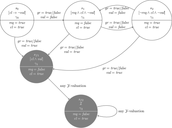
Figure 1: Counterstrategy for specification in Example 1. The logical expressions in square brackets denote the subset of game states corresponding to each counterstrategy state; $\mathcal{I}$ denotes the entire set of possible valuations. The lower half of each state $s$ denotes the next input valuation $E(s)$.

It represents a set of system behaviors where the environment forces the violation of $\phi^{fair}_{\mathcal{S}}$ by keeping the cl variable constantly true, while satisfying $\phi^{fair}_{\mathcal{E}}$ by alternating between $\textit{req}=\textit{true}$ and $\textit{req}=\textit{false}$. ∎

A GR(1) formula $\phi=\phi^{\mathcal{E}}\rightarrow\phi^{\mathcal{S}}$ is realizable if there are no environment strategies that satisfy $\lnot\phi$. This can be achieved either by weakening $\phi^{\mathcal{S}}$, or by strengthening $\phi^{\mathcal{E}}$. Assumptions refinement deals with the latter option.

Definition 6

Given an unrealizable GR(1) formula $\phi=\phi^{\mathcal{E}}\rightarrow\phi^{\mathcal{S}}$, the problem of assumptions refinement requires identifying a set of additional assumptions $\mathbf{\Psi}=\{\psi_{1},\dots,\psi_{k}\}$ such that the refined formula $\phi^{\mathcal{E}}\land\bigwedge_{i=1}^{k}\psi_{i}\rightarrow\phi^{\mathcal{S}}$ is realizable.

We call refinements the additional assumptions $\psi_{i}$. For simplicity, we call realizable refinements those refinements that make $\phi$ realizable, thus solving the realizability problem.

Since a realizable formula is inconsistent with any counterstrategy, and for an unrealizable formula a counterstrategy can be computed automatically Könighofer et al (2009), a general approach to compute $\mathbf{\Psi}$ is to generate a set of assumptions that are inconsistent with such a counterstrategies: these approaches are called counterstrategy-guided assumption refinement and provide a basis for our work.

2.2.3 Abstract counterstrategies

Typically a full description of a counterstrategy is not needed for assumptions refinement, and more concise descriptions are actually employed Alur et al (2013b); Li et al (2011, 2014). The first simplification consists in removing all controller choices that lead to finite-time violations of the guarantees. The second consists in removing from the transition labellings all the output variables whose assignments are not influential to the choice of the next state (such as gr in the above example).

Let $\phi_{\scriptsize\textit{inv}}^{\mathcal{S}}=\textsf{{G}}B^{\scriptsize\textit{inv}}(\mathcal{V}\cup\textsf{{X}}\mathcal{V})$ be the invariant guarantee in an unrealizable GR(1) formula $\phi$ (if the formula has more than one invariant guarantee, we can use the equivalence $\textsf{{G}}B^{\scriptsize\textit{inv}}_{1}\land\textsf{{G}}B^{\scriptsize\textit{inv}}_{2}\equiv\textsf{{G}}(B^{\scriptsize\textit{inv}}_{1}\land B^{\scriptsize\textit{inv}}_{2})$ to ensure $\phi$ has at most one invariant without loss of generality). Given a state $s=(\mathcal{I}_{s},\gamma_{s})\in\mathcal{S}$ of a counterstrategy, with $\mathcal{I}_{s}=\{I_{1},\dots,I_{n}\}$, let $\mathcal{I}_{fail}(s)=\{I:\mathcal{V}\rightarrow\{\textit{true},\textit{false}\}\;|\;I_{\mathcal{X}}=E(s)\land\forall j\in\{1,\dots,n\},p=I_{j}Ip_{2}p_{3}\dots\;p\not\models B^{\scriptsize\textit{inv}}\}$ be the set of all valuations $I$ that cause a violation of the invariant when appearing in a play right after the last valuation $I_{j}$ observed in $s$. We call this the set of failing valuations. Let $\mathcal{I}_{fail,\mathcal{Y}}(s)=\{I_{\mathcal{Y}}:\mathcal{Y}\rightarrow\{\textit{true},\textit{false}\}\;|\;I\in\mathcal{I}_{fail}(s)\}$ the set of the restrictions of the failing valuations to the output variables. Then, let us call $\mathcal{I}_{adm,\mathcal{Y}}(s)=\mathcal{I}_{\mathcal{Y}}\backslash\mathcal{I}_{fail,\mathcal{Y}}(s)$ the set of all controller responses from $s$ that do not cause a violation of the invariant; we call this the set of admissible output assignments from $s$.

Then we can give the following definition of abstract counterstrategy.

Definition 7

An abstract counterstrategy is a 4-tuple $\mathcal{C}=(\mathcal{S},s_{0},E,T)$ such that:

• $\mathcal{S}\subseteq 2^{\mathcal{I}}\times\Gamma$ is a set of states;

• $s_{0}=(\mathcal{I}_{0},\gamma_{0})$ is the initial state;

• $E:\mathcal{S}\rightarrow\mathcal{I}_{\mathcal{X}}$ is the decision function of the environment, that given a current state returns the next input valuation;

• $\mathcal{T}=\{T_{s}\}_{s\in\mathcal{S}}$ is a collection of transition functions, indexed by states in $\mathcal{S}$; for every $s\in\mathcal{S}$, $T_{s}:\mathcal{I}_{adm,\mathcal{Y}}(s)\rightarrow\mathcal{S}$ is a function that, given an admissible output assignment for state $s$, returns the next state.

Example 2

Let us consider again the counterstrategy of Example 1. A first thing to note is that, since the violation regards a fairness condition, the upper part ends in a strongly connected subset of nodes where $\textit{gr}\land\textit{val}$ is false.

Notice also that in each state the choice of the next input does not depend on gr, since the state reached in any transition is the same regardless of the value of gr. Moreover, if at any step the controller chooses to set val to true, the invariant $\phi^{inv}_{\mathcal{S}}$ is violated: therefore the counterstrategy enters the state $s_{f1}$ and from that point any subsequent infinite play is violating.

Formally,

$$\mathcal{I}_{fail,\mathcal{Y}}(s_{0})=\mathcal{I}_{fail,\mathcal{Y}}(s_{1})=\mathcal{I}_{fail,\mathcal{Y}}(s_{2})=\{I_{\mathcal{Y}}\in\mathcal{I}_{\mathcal{Y}}|I_{\mathcal{Y}}(\textit{val})=\textit{true}\}$$

and

$$\mathcal{I}_{adm,\mathcal{Y}}(s_{0})=\mathcal{I}_{adm,\mathcal{Y}}(s_{1})=\mathcal{I}_{adm,\mathcal{Y}}(s_{2})=\{I_{\mathcal{Y}}\in\mathcal{I}_{\mathcal{Y}}|I_{\mathcal{Y}}(\textit{val})=\textit{false}\}$$

According to the new definition, the counterstrategy will appear as in Figure 2.

Figure 2: Counterstrategy of the specification in Example 1 with the alternative definition

∎

We finally define the notion of influential output variable for a state.

Definition 8

We define the set of influential output variables of a state $s$ as $Y(s)=\{y\in\mathcal{Y}\;|\;\forall I_{1,\mathcal{Y}},I_{2,\mathcal{Y}}\in\mathcal{I}_{adm,\mathcal{Y}}(s),\exists I_{1,\mathcal{Y}},I_{2,\mathcal{Y}}\in\mathcal{I}_{\mathcal{Y}}(s)\text{ such that }I_{1,\mathcal{Y}}(y)\neq I_{2,\mathcal{Y}}(y)\land T_{s}(I_{1,\mathcal{Y}})\neq T_{s}(I_{2,\mathcal{Y}})\}$.

The function $Y:\mathcal{S}\rightarrow 2^{\mathcal{Y}}$ maps every state to the set of its influential output variables.

In other words, an influential output variable is a variable whose assignment determines the next state in the counterstrategy. We can provide a more concise description of a counterstrategy by using only influential variables to label transitions.

Example 3

Consider the graph in Figure 2, and the state $s_{0}$. We want to identify the set of influential output variables $Y(s_{0})$.

First, consider the variable val. As shown in the previous example, $I_{\mathcal{Y}}\in\mathcal{I}_{adm,\mathcal{Y}}(s_{0})$ if and only if $I_{\mathcal{Y}}(\textit{val})=\textit{false}$. Therefore, there are no two admissible valuations of val in $\mathcal{I}_{adm,\mathcal{Y}}(s_{0})$, and $\textit{val}\not\in Y(s_{0})$.

Then consider the variable gr. Both true and false appear in some admissible valuations of $s_{0}$, but the next state does not depend on the value assigned to gr. In symbols:

$$\forall I_{1,\mathcal{Y}},I_{2,\mathcal{Y}}\in\mathcal{I}_{adm,\mathcal{Y}}(s_{0})\text{ such that }I_{1,\mathcal{Y}}(\textit{gr})\neq I_{2,\mathcal{Y}}(\textit{gr}),\;T_{s_{0}}(I_{1,\mathcal{Y}})=T_{s_{0}}(I_{2,\mathcal{Y}})\;.$$

Therefore $\textit{gr}\not\in Y(s_{0})$. We can then conclude that there are no influential output variables in $s_{0}$, and $Y(s_{0})=\varnothing$.

Since the same reasoning can be performed on all other states, the description can be reduced to the simple, one-path graph with unlabeled transitions in Figure 3.

Figure 3: Reduced counterstrategy description for specification in Example 1

∎

Any path on an abstract counterstrategy starting from the initial state is called counterrun. It induces a sequence of partial valuations where the subset of variables valuated is different at each step. Given a run $r=s_{0}s_{1}s_{2}\dots$, where $s_{0}$ is the initial state, we define the abstract counterplay (or simply counterplay) $p=I_{0}I_{1}I_{2}\dots$ as a sequence of valuations such that

• $I_{0}\in\mathcal{I}_{0}$

• $\forall i>0,\;I_{i}:\mathcal{X}\cup Y(s_{i-1})\rightarrow\{\textit{true},\textit{false}\}$; that is, the $i$-th valuation is defined over the set of input and influential output variables of state $i-1$

• $\forall i>0,\;T_{s_{i-1}}(I_{i})=s_{i}$.

Counterplays are abstract descriptions of sequences of system states leading to a specific guarantee violation in the counterstrategy. By construction, any play of valuations in $\mathcal{V}$ consistent with an abstract counterplay violates the GR(1) formula $\phi$. Our approach makes use of counterplays to generate assumptions refinements (see Section 4).

2.2.4 Unrealizable cores

GR(1) specifications tend to be lengthy and in this case finding the cause of unrealizability is nontrivial. The concept of unrealizable core defines a subset of GR(1) conjuncts that help explain the cause of unrealizability. We use a slightly different notion of unrealizable core from the one in Cimatti et al (2008b): the original work considered subsetting both assumptions and guarantees, while our definition, following Könighofer et al (2009), considers only subsetting guarantees.

Definition 9

Given an unrealizable GR(1) specification $\phi=\langle\phi^{\mathcal{E}},\phi^{\mathcal{S}}\rangle$, an unrealizable core is a subset $\phi^{uc}\subseteq\phi^{\mathcal{S}}$ such that:

• $\langle\phi^{\mathcal{E}},\phi^{uc}\rangle$ is unrealizable, and

• for every $\phi^{\prime}\subseteq\phi^{uc}$, $\langle\phi^{\mathcal{E}},\phi^{\prime}\rangle$ is realizable.

For performance reasons, counterstrategy graphs are typically computed from unrealizable cores rather than entire specifications.

2.3 Craig Interpolation

Craig interpolation was originally defined for first-order logic Craig (1957) and later for propositional logic Krajíček (1997). No interpolation theorems have been proved for the general LTL. Extensions have been proposed recently for LTL fragments Kamide (2015); Gheerbrant and ten Cate (2009). However these do not include GR(1) formulae and therefore are not applicable in our case. We use interpolation for propositional logic.

Formally, given an unsatisfiable conjunction of formulae $B_{1}(\mathcal{V}_{1})\wedge B_{2}(\mathcal{V}_{2})$, a Craig interpolant $B_{I}(\mathcal{V}_{I})$ is a formula that is implied by $B_{1}$, is unsatisfiable in conjunction with $B_{2}$, and is defined on the common alphabet $\mathcal{V}_{I}$ of $B_{1}$ and $B_{2}$. Recall that a valid Boolean formula is a formula that yields true for any assignment of its variables.

Definition 10 (Interpolant Krajíček (1997))

Let $B_{1}(\mathcal{V}_{1})$ and $B_{2}(\mathcal{V}_{2})$ be two logical formulae such that their conjunction $\mathcal{V}_{1}\wedge\mathcal{V}_{2}$ is unsatisfiable. Then there exists a third formula $B_{I}(\mathcal{V}_{I})$, called interpolant of $B_{1}$ and $B_{2}$, such that, $B_{1}\rightarrow B_{I}$ is valid, $B_{I}\rightarrow\lnot B_{2}$ is valid and $\mathcal{V}_{I}\subseteq\mathcal{V}_{1}\cap\mathcal{V}_{2}$.

An interpolant can be considered as an over-approximation of $B_{1}$ that is still unsatisfiable in conjunction with $B_{2}$. As stated in Craig’s interpolation theorem, although an interpolant always exists, it is not unique. Several efficient algorithms have been proposed for interpolation in propositional logics. The resulting interpolant depends on the internal strategies of these algorithms (e.g., SAT solvers, theorem provers). Our approach is based on McMillan’s interpolation algorithm described in McMillan (2003) and implemented in MathSAT Cimatti et al (2008a). The algorithm considers a proof by resolution for the unsatisfiability of $B_{1}\wedge B_{2}$.

Definition 11 (Unsatisfiability Proof McMillan (2003))

A proof of unsatisfiability for a set of clauses $C$ is a directed acyclic graph $(V,E)$, where the vertices $V$ is a set of clauses, such that for every vertex $c\in V$, either

• $c\in C$, and $c$ is a root, or

• $c$ has exactly two predecessors, $c_{1}$ and $c_{2}$, and $c$ is their resolvent,

and the empty clause false is the unique leaf.

Definition 12 (Interpolation Algorithm McMillan (2003))

Let $B_{1}$ and $B_{2}$ be a pair of clause sets and let $\Pi=(V,E)$ be a proof of unsatisfiability of $B_{1}\wedge B_{2}$ , with leaf vertex false. For all vertices $c\in V$ , let $p(c)$ be a Boolean formula, such that

• if $c$ is a root, then

  • if $c\in B_{1}$ then $p(c)=g(c)$,

  • otherwise $p(c)$ is the constant true.

• else, considering $c_{1}$ and $c_{2}$ are the predecessors of $c$, $v$ their pivot variable,

  • if $v$ is in the language $\mathcal{V}_{1}\backslash\mathcal{V}_{2}$, then $p(c)=p(c_{1})\vee p(c_{2})$,

  • otherwise $p(c)=p(c_{1})\wedge p(c_{2})$.

Then the interpolant is $p(\textit{false})$.

3 Approach Overview

Understanding the cause of unrealizability involves checking some execution of the system, that is one particular sequence of interactions between the environment and the controller, identifying the guarantee(s) that was violated and tracing it back to the input assignments that forced that guarantee(s) to be violated. As a concrete instance of this reasoning, let us consider again the specification from Example 1 and the relevant counterstrategy. In that case, the violated guarantee is $\phi^{fair}_{\mathcal{S}}$, since the output variable val is never true throughout the infinite path. In turn, the invariant guarantee $\phi^{inv}_{\mathcal{S}}$ expresses a relationship between the input variable cl and val, that is, whenever cl is true, val must be false by virtue of the implication. By checking the value of cl along the path, we see cl is always false along the path, hence the violation of $\phi^{fair}_{\mathcal{S}}$. An assumption inconsistent with this behavior would be GFcl, which would make the property realizable.

The first step of the above reasoning, that is identifying a violated guarantee, corresponds to identifying a logical formula to prove; the second step, that is following an implication step to identify a cause of the violation, corresponds to performing a resolution step; finally, the third step of identifying the input variables of interest in the violation corresponds to restraining the cause to the shared alphabet between the assumptions and the guarantees. All these steps are encompassed automatically by Craig interpolation.

The general procedure we propose is based on a sequence of realizability checks and counterstrategy computations, in the spirit of Li et al (2011); Alur et al (2013b), summarized in Algorithm 1. A specification $\langle\phi^{\mathcal{E}},\phi^{\mathcal{S}}\rangle$ is first checked for realizability. If it is unrealizable, a counterstrategy $\mathcal{C}$ and an unrealizable core $\phi^{uc}$ are computed. The counterstrategy constitutes an example of environment behaviours that force the violation of the guarantees of $\phi^{uc}$: therefore, the assumptions $\phi^{\mathcal{E}}$ are refined by adding a GR(1) formula which is inconsistent with the counterstrategy. A set of such formulae $\Psi$ is automatically computed by interpolating ($B_{1}$) the description of an environment behaviour in the counterstrategy, given by the assumptions and a sequence of state labellings in the counterstrategy; and ($B_{2}$) the guarantees. Each formula $\psi_{i}\in\Psi$ derived from the interpolant is conjoined in turn to $\phi^{\mathcal{E}}$ and added to a queue of candidate refinements: then each candidate is checked iteratively for realizability and added to the set of solutions if realizability is achieved; if not, the candidate is further refined and new candidates are added to the queue. In doing this, the procedure produces a tree of candidate refinements, which we will call refinement tree, where every node corresponds to a candidate refinement and the leaves correspond to the realizable solutions. The structure of a refinement tree is pictured in Figure 4. By exploring the queue with a first-in-first-out policy, the procedure implements a breadth-first search of the refinement tree.

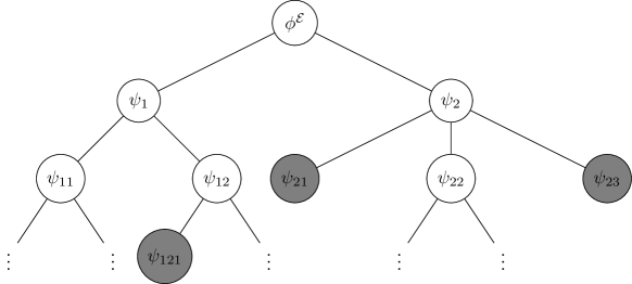
Figure 4: A refinement tree. The refinement corresponding to each node is the conjunction of the $\psi_{i}$ in the node with all its ancestors up to the root. The grey nodes are realizable leaves.

Data: $\phi^{\mathcal{E}}$, assumptions

Data: $\phi^{\mathcal{S}}$, guarantees

Result: $refinements=\{\phi^{\mathcal{E}}\land\psi_{i}\}$, set of alternative refined assumptions such that $\phi^{\mathcal{E}}\land\psi_{i}\rightarrow\phi^{\mathcal{S}}$ is realizable for every $i$

1 $candidateRefQueue\leftarrow\{\phi^{\mathcal{E}}\}$;

2 repeat

3       $candidateRef\leftarrow candidateRefQueue$.pop();

4       if IsSatisfiable($candidateRef$) and $\lnot$IsRealizable($candidateRef\rightarrow\phi^{\mathcal{S}}$) then

5             $\phi^{uc}\leftarrow$ getUnrealizableCore$(candidateRef,\phi^{\mathcal{S}})$;

6             $\mathcal{C}\leftarrow$ getCounterstrategy$(candidateRef,\phi^{\mathcal{S}})$;

7             $\mathbf{\Psi}\leftarrow$ InterpolationBasedSynthesis$(candidateRef,\phi^{uc},\mathcal{C})$;

8             foreach $\psi_{i}\in\mathbf{\Psi}$ do

9                   $candidateRefQueue$.append($candidateRef\land\psi_{i}$);

10                  

11             end foreach

12            

13       else if IsSatisfiable($candidateRef$) then

14             $refinements$.append($candidateRef$);

15            

16      

17until $candidateRefQueue=\varnothing$;

18return $refinements$;

Algorithm 1 CounterstrategyGuidedRefinement procedure

The function InterpolationBasedSynthesis constitutes the core of our proposal (see Algorithm 2). It takes as inputs an unrealizable core and a counterstrategy and executes the computation of $\Psi$ via interpolation. We give the details in the following section.

Data: $\phi^{\mathcal{E}}$, environment assumptions

Data: $\phi^{uc}$, controller guarantees (in an unrealizable core)

Data: $\mathcal{C}$, counterstrategy

Result: ${\Psi}$, alternative assumptions eliminating the counterstrategy

1 $r_{\mathcal{C}}$ := ExtractCounterrun($\mathcal{C}$);

2 $\llbracket\mathcal{V},\phi^{\mathcal{E}}\rrbracket_{r}$:= TranslateCounterrunAssumptions($r_{\mathcal{C}}$, $\phi^{\mathcal{E}}$);

3 $\llbracket\phi^{uc}\rrbracket_{r}$ := TranslateGuarantees($r_{\mathcal{C}}$,$\varphi^{\mathcal{S}}$);

4 $I$ := Interpolate($\llbracket\mathcal{V},\phi^{\mathcal{E}}\rrbracket_{r}$, $\llbracket\phi^{uc}\rrbracket_{r}$);

5 if  $I$ == false or $I$ is not fully-separable then

6       ${\Psi}$ := $\{\textit{false}\}$;

7      

8else

9       $\mathcal{T}(I)$ := TranslateInterpolant($r_{\mathcal{C}}$, $I$);

10       ${\Psi}$ := ExtractDisjuncts($\lnot\mathcal{T}(I)$);

11       return ${\Psi}$;

12      

13 end if

Algorithm 2 InterpolationBasedSynthesis($\phi^{\mathcal{E}}$, $\phi^{uc}$, $\mathcal{C}$)

4 Interpolation-Based Synthesis

Each execution of InterpolationBasedSynthesis involves extracting temporal formulae that are satisfied by a single run of a counterstrategy (a counterrun), and obtaining refinements from their negation. Excluding a single counterrun is sufficient to make the counterstrategy inconsistent with the refined assumptions. Reasoning about counterruns rather than whole counterstrategies has also some advantages, which are discussed in Sect. 7. For the purpose of this paper, we assume that the procedure ExtractCounterrun (line 2) extracts a counterrun $r_{\mathcal{C}}$ at random.

A counterrun leading to the violation of an initial condition or an invariant guarantee is finite, while that of a fairness guarantee violation ends in a loop Li et al (2014). We call the latter a looping counterrun, and the loop an ending loop.

A counterrun consists of four sets of states: (a) the initial state as the element of the singleton $\mathcal{S}^{init}=\{s_{0}\}$; (b) the failing state in a finite counterrun as the element of $\mathcal{S}^{fail}=\{s^{fail}\}$ (c) looping states that include the states in ending loop, $\mathcal{S}^{loop}=\{s^{loop}_{1},\dots,s^{loop}_{h}\}$, (d) transient states including all states between the initial state and the first failing state or loop state (exclusive) $\mathcal{S}^{trans}=\{s^{trans}_{1},\dots,s^{trans}_{k}\}$. With this classification, a finite counterrun has the form $r_{\mathcal{C}}=s_{0}s^{trans}_{1}\dots s^{trans}_{k}s^{fail}$; whilst a looping counterrun has the form $r_{\mathcal{C}}=s_{0}s^{trans}_{1}\dots s^{trans}_{k}(s^{loop}_{1}\dots s^{loop}_{h})^{\omega}$. We call $\mathcal{S}_{r}\subseteq\mathcal{S}$ the union of all the states appearing in $r_{\mathcal{C}}$.

Example 4

Let us consider the specification in Example 1 and the counterstrategy in Figure 3. The counterstrategy has only one looping run $r_{\mathcal{C}}=s_{0}(s_{1}s_{2})^{\omega}$, which is to be used at next stages. This is an example of a looping counterrun with $\mathcal{S}^{init}=\{s_{0}\},\mathcal{S}^{trans}=\varnothing,\mathcal{S}^{loop}=\{s_{1},s_{2}\}$, and $\mathcal{S}_{r}=\mathcal{S}=\{s_{0},s_{1},s_{2}\}$. ∎

Candidate assumption refinements are computed in four steps: (i) production of two inconsistent Boolean formulae from the counterplay and the unrealizable core, (ii) interpolation between the two Boolean formulae, (iii) translation of the interpolant into LTL, and (iv) negation of the translated interpolant.

4.1 Boolean Descriptions of Counterplays and Unrealizable Cores

Step (i) is implemented by the functions TranslateCounterrunAssumptions and TranslateGuarantees (lines 2-2). The procedure employs a similar translation scheme as defined in Biere et al (2003) for bounded model checking, which ensures that the obtained Boolean formula is satisfiable if and only if the play taken into account satisfies the LTL formula.

The translation of a GR(1) formula into the Boolean domain is a Boolean formula over the domain $\mathcal{V}(\mathcal{S}_{r})$ obtained by replicating every variable $v\in\mathcal{V}$ for every state $s\in\mathcal{S}_{r}$; we denote by $v(s)$ the replica of $v$ referring to state $s$, and by $\mathcal{V}(s)$ the subset of $\mathcal{V}(\mathcal{S}_{r})$ containing all the variables referring to state $s$. Formally:

$$\mathcal{V}(\mathcal{S}_{r}):=\{v(s)|v\in\mathcal{V},\;s\in\mathcal{S}_{r}\}$$

$$\forall s\in\mathcal{S}_{r},\;\mathcal{V}(s):=\{v(s)|v\in\mathcal{V}\}$$

The translation operation is designed so as to be executed in linear time with the length of $r_{\mathcal{C}}$, and works on GR(1) conjuncts as follows:

• an initial condition $\varphi^{\theta}_{init}=B^{{\scriptsize\textit{init}}}(\mathcal{V})$ is translated to $\llbracket\varphi^{\theta}_{init}\rrbracket_{r}:=B^{{\scriptsize\textit{init}}}(\mathcal{V}(s_{0}))$ by replacing each occurrence of $v\in\mathcal{V}$ with $v(s_{0})\in\mathcal{V}(s_{0})$;

• an invariant $\varphi^{\theta}_{inv}=\textsf{{G}}B^{{\scriptsize\textit{inv}}}(\mathcal{V}\cup\textsf{{X}}\mathcal{V})$ is translated as the conjunction over all states in $\mathcal{S}_{r}$ $\llbracket\varphi^{\theta}_{inv}\rrbracket_{r}:=\bigwedge_{s\in\mathcal{S}_{r}}B^{{\scriptsize\textit{inv}}}(\mathcal{V}(s)\cup\mathcal{V}(\operatorname{succ}{(s)}))$, where $\operatorname{succ}(s)$ is the successor state of $s$;

• a fairness condition $\varphi^{\theta}_{fair}=B^{fair}(\mathcal{V})$ is translated into a disjunction over the looping states as $\llbracket\varphi^{\theta}_{fair}\rrbracket_{r}:=\bigvee_{s\in\mathcal{S}^{loop}}B^{fair}(\mathcal{V}(s))$, or skipped if $r_{\mathcal{C}}$ is not looping.

The translation produces two Boolean formulae: a formula $\llbracket\mathcal{V},\phi^{\mathcal{E}}\rrbracket_{r}:=\llbracket\phi^{\mathcal{E}}\rrbracket_{r}\land\llbracket\mathcal{V}\rrbracket_{r}$ that describes $r_{\mathcal{C}}$ and a formula $\llbracket\phi^{uc}\rrbracket_{r}$ that describes the unrealizable core. The former consists of two conjuncts:

• a Boolean expression $\llbracket\phi^{\mathcal{E}}\rrbracket_{r}$ that translates the assumptions by the rules described above;

• a Boolean expression $\llbracket\mathcal{V}\rrbracket_{r}$ describing the input and output valuations last seen at every state $s$ in $r_{\mathcal{C}}$, restraining the output valuation to the influential output variables for the predecessor of $s$.

The expression $\llbracket\mathcal{V}\rrbracket_{r}=\land_{s\in\mathcal{S}_{r}\backslash\mathcal{S}^{init}}B(\mathcal{V}(s))$ is a conjunction of formulae whose variables refer to a single state $s$. Each $B(\mathcal{V}(s))$ is a conjunction of literals $v(s)$ or $\lnot v(s)$ for every $v\in\mathcal{X}\cup Y(\operatorname{pred}(s))$, where $\operatorname{pred}(s)$ is the predecessor of $s$ in $r_{\mathcal{C}}$; the formula contains the positive literal $v(s)$ if and only if $E(\operatorname{pred}(s))(v)=\textit{true}$, when $v$ is an input variable, or $I_{\mathcal{Y}}(v)=\textit{true}$ for $T_{\operatorname{pred}(s)}(I_{\mathcal{Y}})=s$, when $v$ is an influential output variable for $\operatorname{pred}(s)$; dually, the formula contains the negative literal $\lnot v(s)$ if and only if $E(\operatorname{pred}(s))(v)=\textit{false}$, when $v$ is an input variable, or $I_{\mathcal{Y}}(v)=\textit{false}$ for $T_{\operatorname{pred}(s)}(I_{\mathcal{Y}})=s$, when $v$ is an influential output variable for $\operatorname{pred}(s)$. Since by construction the counterplay satisfies the assumptions $\phi^{\mathcal{E}}$, the formula $\llbracket\mathcal{V},\phi^{\mathcal{E}}\rrbracket_{r}$ is satisfiable.

The formula $\llbracket\phi^{uc}\rrbracket_{r}$ only contains the translation of the unrealizable core obtained via the rules described above. Since by definition a counterrun $r_{\mathcal{C}}$ satisfies the assumptions and violates the guarantees, the formula $\llbracket\mathcal{V},\phi^{\mathcal{E}}\rrbracket_{r}\land\llbracket\phi^{uc}\rrbracket_{r}$ is unsatisfiable by construction. Therefore, there exists an interpolant for $\llbracket\mathcal{V},\phi^{\mathcal{E}}\rrbracket_{r}$ and $\llbracket\phi^{uc}\rrbracket_{r}$.

Example 5

In the request-grant protocol, the assumption $\phi^{fair}_{\mathcal{E}}=\textsf{{G}}\textsf{{F}}\lnot\textit{req}$ is translated as:

$$\llbracket\phi^{fair}_{\mathcal{E}}\rrbracket_{r}=\lnot\textit{req}(s_{1})\lor\lnot\textit{req}(s_{2})$$

Since there is just one assumption, $\llbracket\phi^{\mathcal{E}}\rrbracket_{r}=\llbracket\phi^{fair}_{\mathcal{E}}\rrbracket_{r}=\lnot\textit{req}(s_{1})\lor\lnot\textit{req}(s_{2})$ The formula $\llbracket\mathcal{V}\rrbracket_{r}$ is obtained by inspecting Figure 3 for the last valuations of input and influential output variables in each state:

$$\llbracket\mathcal{V}\rrbracket_{r}=(\textit{req}(s_{1})\land\textit{cl}(s_{1}))\land(\lnot\textit{req}(s_{2})\land\textit{cl}(s_{2}))\;.$$

The Boolean description of the counterplay is just $\llbracket\mathcal{V},\phi^{\mathcal{E}}\rrbracket_{r}=\llbracket\phi^{\mathcal{E}}\rrbracket_{r}\land\llbracket\mathcal{V}\rrbracket_{r}$.

The translation of the invariant guarantee $\phi^{inv}_{\mathcal{S}}=\textsf{{G}}(\textit{cl}\rightarrow\lnot\textit{val})$ is:

$$\llbracket\phi^{inv}_{\mathcal{S}}\rrbracket_{r}=(\textit{cl}(s_{0})\rightarrow\lnot\textit{val}(s_{0}))\land(\textit{cl}(s_{1})\rightarrow\lnot\textit{val}(s_{1}))\land(\textit{cl}(s_{2})\rightarrow\lnot\textit{val}(s_{2}))\;.$$

That of the fairness guarantee $\phi^{fair}_{\mathcal{S}}=\textsf{{G}}\textsf{{F}}(\textit{gr}\land\textit{val})$:

$$\llbracket\phi^{fair}_{\mathcal{S}}\rrbracket_{r}=(\textit{gr}(s_{1})\land\textit{val}(s_{1}))\lor(\textit{gr}(s_{2})\lor\textit{val}(s_{2}))\;.$$

Hence, the translation of the guarantees is just

$$\llbracket\phi^{uc}\rrbracket_{r}=\llbracket\phi^{inv}_{\mathcal{S}}\rrbracket_{r}\land\llbracket\phi^{fair}_{\mathcal{S}}\rrbracket_{r}$$

∎

4.2 Interpolation and Full Separability

Step (ii) consists of the function Interpolate (line 2). The returned interpolant $I$ is an over-approximation of $\llbracket\mathcal{V},\phi^{\mathcal{E}}\rrbracket_{r}$ which by definition implies the negation of $\llbracket\phi^{uc}\rrbracket_{r}$: it can be interpreted as a cause of the guarantees not being satisfied by the counterplay, and as such a characterization of a set of counterplays not satisfying the guarantees.

From such interpolant the procedure aims at extracting a set of refinements that fit the GR(1) format. In order to do this, the Boolean to temporal translation requires the interpolant to adhere a specific structure. This is embodied in the notion of full-separability. To formally define full-separability, we need first to define state-separability and I/O-separability.

Definition 13 (State-separable interpolant)

An interpolant $I$ is said to be state-separable iff it is in the form

$$\bigwedge_{s\in\mathcal{S}_{r}}B_{s}(\mathcal{V}(s))$$ (1)

where $B_{s}(\mathcal{V}(s))$ is a Boolean formula either equal to true or expressed over variables in $\mathcal{V}(s)$ only.

We will refer to each $B_{s}(\mathcal{V}(s))$ as a state component of the interpolant. In particular, a state component is equal to true if $I$ does not use any variables from $s$. State-separability intuitively means that the subformulae of the interpolant involving every single state in the counterplay are linked by conjunctions. This means that in any model of the interpolant each state component must be itself true.

Definition 14 (I/O-separable Boolean expression)

A Boolean expression $B_{s}(\mathcal{V}(s))$ is said to be I/O-separable if it can be written as a conjunction of two subformulae containing only input and output variables respectively:

$$B_{s}(\mathcal{V}(s))=B_{s,\mathcal{X}}(\mathcal{X}(s))\land B_{s,\mathcal{Y}}(\mathcal{Y}(s))$$ (2)

We call $B_{s,\mathcal{X}}(\mathcal{X}(s))$ and $B_{s,\mathcal{Y}}(\mathcal{Y}(s))$ the projections of $B_{s}(\mathcal{V}(s))$ onto $\mathcal{X}$ and $\mathcal{Y}$ respectively. Any model of an I/O-separable Boolean expression satisfies the projections separately. We can now define full-separability of an interpolant.

Definition 15 (Fully-separable interpolant)

An interpolant is called fully-separable if it is state-separable and each of its state components is I/O-separable.

An example of a fully-separable interpolant over $\mathcal{X}=\{a,b\},\mathcal{Y}=\{c,d\}$ and states $S=\{s_{0},s_{1}\}$ is $(a(s_{0})\lor b(s_{0}))\land c(s_{0})\land\lnot b(s_{1})$; a non-fully-separable interpolant, instead, is $a(s_{0})\lor a(s_{1})$, since literals referring to different states are linked via a disjunction.

Remark 1

A particular class of fully-separable interpolants is that of fully conjunctive interpolants, where no disjunctions appear. Whether or not the resulting interpolant is conjunctive depends on the order in which the interpolation algorithm McMillan (2003) chooses the root clauses for building the unsatisfiability proof. A sufficient condition for obtaining a fully-conjunctive interpolant is that such root clauses be single literals from $\llbracket\mathcal{V},\phi^{\mathcal{E}}\rrbracket_{r}$, and that the pivot variable in each resolution step belong to the shared alphabet of $\llbracket\mathcal{V},\phi^{\mathcal{E}}\rrbracket_{r}$ and $\llbracket\phi^{uc}\rrbracket_{r}$ (see Section 2.3).

Example 6

The interpolant of $\llbracket\mathcal{V},\phi^{\mathcal{E}}\rrbracket_{r}$ and $\llbracket\phi^{uc}\rrbracket_{r}$ from Example 5 is $I=\textit{cl}(s_{1})\land\textit{cl}(s_{2})$, which is fully separable. Notice that $I$ captures the environment’s choices that cause the violation: cl being always true in the looping states $s_{1}$ and $s_{2}$. ∎

4.3 Interpolant Translation

Step (iii) consists of the function TranslateInterpolant (line 2). It converts a fully-separable interpolant $I=\bigwedge_{s\in\mathcal{S}_{r}}B_{s}(\mathcal{V}(s))$ into the LTL formula

$$\begin{split}\mathcal{T}(I):=&B^{init}_{\mathcal{X}}(\mathcal{X})\land\bigwedge_{s\in\mathcal{S}_{r}}\textsf{{F}}\left(B_{s}(\mathcal{V})\land B_{\operatorname{succ}{(s)},\mathcal{X}}(\textsf{{X}}\mathcal{X})\right)\land\\ &\textsf{{F}}\textsf{{G}}\bigvee_{j=1}^{|\mathcal{S}^{loop}|}B^{loop}_{j}(\mathcal{V})\end{split}$$ (3)

where the expression $B^{init}_{\mathcal{X}}(\mathcal{X})$ is a shorthand for $B_{s_{0},\mathcal{X}}(\mathcal{X})$ and $B^{loop}_{j}(\mathcal{V})$ for $B_{s^{loop}_{j}}(\mathcal{V})$. Formula (3) is formed from the single state components of $I$ by replacing the variables in $\mathcal{V}(s)$ with the corresponding variables in $\mathcal{V}$ and by projecting the components onto the input variables where required by the GR(1) template. The translation consists of three units: a subformula describing the initial state, a conjunction of F formulae each containing two consecutive state components, and an FG formula derived from the looping state components of $I$.

Formula (3) is guaranteed to hold in the counterplay $r_{\mathcal{C}}$. Intuitively, since $I$ is fully-separable by construction, $\llbracket\mathcal{V},\phi^{\mathcal{E}}\rrbracket_{r}$ implies each state component and its projections onto $\mathcal{X}$ and $\mathcal{Y}$. A state component $B_{s}(\mathcal{V}(s))$ corresponds to a formula $B_{s}(\mathcal{V})$ satisfied by state $s$ of the counterplay. Therefore, since the initial state satisfies $B^{init}(\mathcal{V})$, $r_{\mathcal{C}}$ satisfies $B^{init}_{\mathcal{X}}(\mathcal{X})$; since there are two consecutive states $s$ and $\operatorname{succ}{(s)}$ that satisfy $B_{s}(\mathcal{V}(s))$ and $B_{s}(\mathcal{V}(\operatorname{succ}{(s)}))$ respectively, $r_{\mathcal{C}}$ satisfies $\textsf{{F}}\left(B_{s}(\mathcal{V})\land B_{\operatorname{succ}{(s)},\mathcal{X}}(\textsf{{X}}\mathcal{X})\right)$. Finally, for the FG subformula, it is sufficient to observe that the looping state $j$ satisfies the formula $B^{loop}_{j}(\mathcal{V})$: since the counterplay remains indefinitely in each of the looping states, there is a suffix of it where such formula is true for at least one $j$. Based on these considerations, we prove the following soundness property.

Theorem 4.1

Let $r_{\mathcal{C}}$ be a counterplay and $\phi^{\mathcal{E}}$ a set of assumptions satisfied in $r_{\mathcal{C}}$, such that their Boolean translation $\llbracket\mathcal{V},\phi^{\mathcal{E}}\rrbracket_{r}$ implies $I$, and let $I$ be a fully-separable interpolant. Then $r_{\mathcal{C}}\models\mathcal{T}(I)$.

Proof

Since we are assuming that $I$ is state-separable, and since by definition $\llbracket\mathcal{V},\phi^{\mathcal{E}}\rrbracket_{r}$ implies $I$, each state component (which is a conjunct in $I$) is implied by $\llbracket\mathcal{V},\phi^{\mathcal{E}}\rrbracket_{r}$:

$$\llbracket\mathcal{V},\phi^{\mathcal{E}}\rrbracket_{r}\rightarrow I\rightarrow B_{s}(\mathcal{V}(s))$$ (4)

for every $s$. By construction, a state component holds true iff it is satisfied by the corresponding state in the counterrun:

$$\llbracket\mathcal{V},\phi^{\mathcal{E}}\rrbracket_{r}\rightarrow B_{s}(\mathcal{V}(s))\Leftrightarrow\langle r_{\mathcal{C}},s\rangle\models B_{s}(\mathcal{V})$$ (5)

Now let us consider $s_{0}$. By (5) and I/O-separability:

$$\begin{split}\llbracket\mathcal{V},\phi^{\mathcal{E}}\rrbracket_{r}\rightarrow B^{init}(V(s_{0}))\Rightarrow&\langle r_{\mathcal{C}},s_{0}\rangle\models B^{init}(V)\\ \Rightarrow&\langle r_{\mathcal{C}},s_{0}\rangle\models B^{init}_{\mathcal{X}}(\mathcal{X})\land B^{init}_{\mathcal{Y}}(\mathcal{Y})\\ \Rightarrow&r_{\mathcal{C}}\models B^{init}_{\mathcal{X}}(\mathcal{X})\end{split}$$ (6)

So, $r_{\mathcal{C}}$ satisfies the part of the translation that refers to the initial state.

The next step is to consider pairs of consecutive states $s$ and $\operatorname{succ}{(s)}$. Since $I_{u}$ is I/O-separable, we have

$$B_{\operatorname{succ}(s)}(\mathcal{V}(\operatorname{succ}(s)))\rightarrow B_{\operatorname{succ}(s),\mathcal{X}}(\mathcal{X}(\operatorname{succ}(s)))$$

By (5) and LTL satisfaction definition for $\mathbf{X}$:

$$\begin{split}\llbracket\mathcal{V},\phi^{\mathcal{E}}\rrbracket_{r}\rightarrow B_{\operatorname{succ}(s),\mathcal{X}}(\mathcal{X}(\operatorname{succ}(s)))\Rightarrow&\langle r_{\mathcal{C}},\operatorname{succ}(s)\rangle\models B_{\operatorname{succ}(s),\mathcal{X}}(\mathcal{X})\\ \Rightarrow&\langle r_{\mathcal{C}},s\rangle\models\mathbf{X}B_{\operatorname{succ}(s),\mathcal{X}}(\mathcal{X})\\ \Rightarrow&\langle r_{\mathcal{C}},s\rangle\models B_{\operatorname{succ}(s),\mathcal{X}}(\mathbf{X}\mathcal{X})\end{split}$$ (7)

From the conjunction of (5) and (7), and from the LTL interpretation of the operator $\mathbf{F}$ we finally get

$$\begin{split}\llbracket\mathcal{V},\phi^{\mathcal{E}}\rrbracket_{r}\rightarrow&B_{s}(\mathcal{V}(s))\land B_{\operatorname{succ}(s)}(\mathcal{V}(\operatorname{succ}(s)))\\ \Rightarrow&\langle r_{\mathcal{C}},s\rangle\models B_{s}(\mathcal{V})\land B_{\operatorname{succ}(s),\mathcal{X}}(\mathbf{X}\mathcal{X})\\ \Rightarrow&r_{\mathcal{C}}\models\mathbf{F}\left(B_{s}(\mathcal{V})\land B_{\operatorname{succ}{(s)},\mathcal{X}}(\mathbf{X}\mathcal{X})\right)\end{split}$$ (8)

Therefore $r_{\mathcal{C}}$ satisfies the “eventually” subformulae in the translation.

Finally, let us consider the looping and unrolled states. In general, a path ending with a loop among states $s_{1},\dots,s_{|\mathcal{S}^{loop}|}$ satisfies the formula

$$\mathbf{FG}\bigvee_{j=1}^{|\mathcal{S}^{loop}|}B_{j}(\mathcal{V})$$ (9)

where $B_{j}$ is any Boolean expression that holds in $s_{j}$. The reason is that there is a suffix of the path that contains only states from $\mathcal{S}^{loop}$; therefore, this suffix always satisfies any of the looping states’ valuations.

Hence, given

$$\langle r_{\mathcal{C}},s^{loop}_{j}\rangle\models B^{loop}_{j}(\mathcal{V})$$ (10)

this can be replaced to the formula in (9) and we obtain:

$$r_{\mathcal{C}}\models\mathbf{F}\mathbf{G}\bigvee_{j=1}^{|S^{loop}|}B^{loop}_{j}(\mathcal{V})$$ (11)

Since $r_{\mathcal{C}}$ satisfies each of the conjuncts in (3), then $r_{\mathcal{C}}\models\mathcal{T}(I)$. ∎

In the case a fully-separable interpolant is not generated from which $\mathcal{T}(I)$ can be constructed, the algorithm returns false as its candidate assumption. Otherwise, the approach proceeds to step (iv) (function ExtractDisjuncts, line 2) producing the candidate refinements by negating (3) and extracting the disjuncts in the resulting formula:

$$\begin{split}\lnot B^{init}_{\mathcal{X}}(\mathcal{X})\lor\bigvee_{s\in S_{u}}\textsf{{G}}\lnot\left(B_{s}(\mathcal{V})\land B_{\operatorname{succ}{(s)},\mathcal{X}}(\textsf{{X}}\mathcal{X})\right)\lor\\ \textsf{{G}}\textsf{{F}}\bigwedge_{j=1}^{|\mathcal{S}^{loop}|}\lnot B^{loop}_{j}(\mathcal{V})\end{split}$$ (12)

Each disjunct above is a GR(1) candidate assumption which, by Theorem 4.1, ensures the exclusion of the counterplay $r_{\mathcal{C}}$ from the models of the assumptions.

4.4 Unrolling

Data: $\phi^{\mathcal{E}}$, environment assumptions

Data: $\phi^{uc}$, controller guarantees (in an unrealizable core)

Data: $\mathcal{C}$, counterstrategy

Result: ${\Psi}$, alternative assumptions eliminating the counterstrategy

1 $r_{\mathcal{C}}$ := ExtractCounterrun($\mathcal{C}$);

2 $u$ := 0;

3 $r_{\mathcal{C},u}$ := $r_{\mathcal{C}}$;

4 ${\Psi_{old}}$ := $\emptyset$;

5 repeat

6       $\llbracket\mathcal{V},\phi^{\mathcal{E}}\rrbracket_{r}$:= TranslateCounterrunAssumptions($r_{\mathcal{C},u}$, $\phi^{\mathcal{E}}$);

7       $\llbracket\phi^{uc}\rrbracket_{r}$ := TranslateGuarantees($r_{\mathcal{C},u}$,$\phi^{uc}$);

8       $I_{u}$ := Interpolate($\llbracket\mathcal{V},\phi^{\mathcal{E}}\rrbracket_{r}$, $\llbracket\phi^{uc}\rrbracket_{r}$);

9       if  $I_{u}=\textit{false}$ or $I_{u}$ is not fully-separable then

10             ${\Psi}$ := $\{\textit{false}\}$;

11             stopping_condition := CheckStoppingCondition($\Psi,\Psi_{old},u$);

12            

13      else

14             $\mathcal{T}(I_{u})$ := TranslateUnrolledInterpolant($r_{\mathcal{C},u}$, $I_{u}$);

15             ${\Psi}$ := ExtractDisjuncts($\lnot\mathcal{T}(I_{u})$);

16             if $r_{\mathcal{C},u}$ is looping then

17                   ${\Psi_{old}}$ := ${\Psi}$;

18                   $u$ := $u+1$;

19                   $r_{\mathcal{C},u}$ := UnrollCounterrun($r_{\mathcal{C}}$,$u$);

20                   $stopping\_condition$ := CheckStoppingCondition($\Psi,\Psi_{old},u$);

21                  

22            else

23                   stopping_condition := true;

24                  

25             end if

26            

27       end if

28      

29until stopping_condition;

30 return ${\Psi}$;

Algorithm 3 InterpolationBasedSynthesis($\varphi^{\mathcal{E}}$, $\varphi^{\mathcal{S}}$, $C$) with unrolling

A common problem to assumptions refinement approaches is that of the vacuity of the refined assumptions Beer et al (2001). A GR(1) specification is said to be vacuously realizable if its assumptions are unsatisfiable; in this case any controller satisfies the specification, since the assumptions evaluate to false. In some cases assumptions refinement approaches trivially eliminate counterstrategies by adding a refinement $\psi$ that is inconsistent with previous assumptions, making the specification vacuously realizable.

Interpolation-based synthesis produces a number of assumptions that grows proportionally with the number of state components in the interpolant, and thereby with the number of states in the counterrun. If the counterrun is small, few refinements are produced and all of them may be inconsistent with the original assumptions. In this case, counterrun unrolling can help producing additional assumptions.

Counterrun unrolling consists in making the first traversals of looping states explicit. It is achieved by augmenting a counterplay with replicates of the looping states. The number of unrollings is referred to as the unrolling degree $u$. Each unrolling yields a new set of states $\mathcal{S}^{unr}=\{s^{unr}_{1,1},\dots,s^{unr}_{h,1},\dots,$ $s^{unr}_{1,u},$ $\dots,s^{unr}_{h,u}\}$. An unrolled looping counterrun has the form $s_{0}s^{trans}_{1}\dots s^{trans}_{k}$ $s^{unr}_{1,1}\dots s^{unr}_{h,1}\dots s^{unr}_{1,u}\dots s^{unr}_{h,u}(s^{loop}_{1}\dots s^{loop}_{k})^{\omega}$. Unrolling has two possible effects on the computed interpolant: on one hand, it can introduce new state components in the interpolant, which yield new invariant refinements according to (12); on the other hand, the interpolant can express a more specific characterization of looping states, which corresponds to a weaker fairness refinement in (12). These effects are both observed in our evaluation (see Sect. 6).

The translation from the temporal to the Boolean domain (lines 3-3) works as in Algorithm 2. When an interpolant is computed, provided that it is fully separable, it can contain components referring to the unrolled states. The state component referring to the $r$-th replica of the $j$-th looping state is denoted by $B^{unr}_{j,r}(\mathcal{V}(s^{unr}_{j,r}))$. The function TranslateUnrolledInterpolant (line 3) produces the formula

$$\begin{split}\mathcal{T}(I_{u}):=&B^{init}_{\mathcal{X}}(\mathcal{X})\land\bigwedge_{s\in\mathcal{S}_{r}}\textsf{{F}}\left(B_{s}(\mathcal{V})\land B_{\operatorname{succ}{(s)},\mathcal{X}}(\textsf{{X}}\mathcal{X})\right)\land\\ &\textsf{{F}}\textsf{{G}}\bigvee_{j=1}^{|\mathcal{S}^{loop}|}\left(B^{loop}_{j}(\mathcal{V})\land\bigwedge_{r=1}^{u}B^{unr}_{j,r}(\mathcal{V})\right)\end{split}$$ (13)

This formula is the same as 3 apart from the FG conjunct. This is replaced with a stronger disjunction, where each disjunct groups the state components referring to all the replicates of the same looping state. By negating (3), the algorithm produces

$$\begin{split}\lnot B^{init}_{\mathcal{X}}(\mathcal{X})\lor\bigvee_{s\in S_{u}}\textsf{{G}}\lnot\left(B_{s}(\mathcal{V})\land B_{\operatorname{succ}{(s)},\mathcal{X}}(\textsf{{X}}\mathcal{X})\right)\lor\\ \textsf{{G}}\textsf{{F}}\bigwedge_{j=1}^{|\mathcal{S}^{loop}|}\lnot\left(B^{loop}_{j}(\mathcal{V})\land\bigwedge_{r=1}^{u}B^{unr}_{j,r}(\mathcal{V})\right)\end{split}$$ (14)

where each disjunct is a candidate refinement, and the fairness condition has a weaker form than the one in (12).

Unrolling is stopped when some user-defined stopping condition is reached. This is checked by the function CheckStoppingCondition. Possible stopping conditions are:

• the interpolant has yielded the same refinements as the previous step;

• no new refinements have been produced in the last $k$ unrolling step;

• a maximum unrolling degree has been specified.

5 Convergence

Our procedure is guaranteed to terminate after a finite number of iterations. We discuss below the case of all computed interpolants being fully-separable. If at some step the interpolant is not fully separable, the InterpolationBasedSynthesis procedure returns the vacuous refinement false, which ensures that branch of the refinement tree is not expanded further.

Theorem 5.1

Given a satisfiable but unrealizable specification $\langle\phi^{\mathcal{E}},\phi^{\mathcal{S}}\rangle$ Algorithm 1 terminates with a realizable specification $\langle\phi^{\mathcal{E}^{\prime}},\phi^{\mathcal{S}}\rangle$.

Proof

To prove this, it is sufficient to show that the iteration in Algorithm 1 reaches its termination conditions. The argument we carry out mirrors the one for proving the termination of Abstract Learning Framework algorithms presented in Löding et al (2016).

In the following arguments, we will refer to the recursion tree of Algorithm 1. Each node is associated with the candidate assumption tested in one specific call of CounterstrategyGuidedRefinements. The root corresponds to the initial assumption; every internal node symbolizes an unrealizable assumptions refinement; the children of an internal node correspond to the alternative refinements that rule out the relevant counterstrategy. The leaves represent alternative realizable assumption refinements returned by the algorithm. We will show that this tree has finite depth and breadth.

Let us consider the number of children $n_{\mathcal{C}}$ of an internal node (the subscript $\mathcal{C}$ refers to the counterstrategy computed in that internal node). It corresponds to the maximum number of refinements that are generated from a single counterstrategy. Formula (12) allows the extraction of one initial condition, one fairness condition and $|\mathcal{S}_{p}|$ invariants; therefore:

$$n_{\mathcal{C}}=|\mathcal{S}_{r}|+2\;.$$

We now consider the depth. The algorithm keeps refining a computed assumption until the property becomes realizable (in case the returned refinement is false, then the property is realizable). Given the soundness property (Theorem 4.1), at each step every refinement excludes the latest computed counterstrategy; since this counterstrategy satisfies all the previously computed refinements by definition, the new refinement cannot be equivalent to any of the previous refinements along the same branch.

For the above reason, the depth $d$ of the refinement tree is limited by the maximum number of existing GR(1) refinements modulo logical equivalence. The maximum number of initial conditions is $d_{init,MAX}=2^{2^{|\mathcal{X}|}}$, that is the number of all distinct Boolean expressions over the input variables. The maximum number of invariants is $d_{inv,MAX}=2^{2^{|\mathcal{V}|}+2^{|\mathcal{X}|}}$; this corresponds to the maximum number of distinct $B_{s}$ that can be present in the expression (12) times the number of distinct $B_{\operatorname{succ}{(s)},X}$. Finally, the maximum number of distinct fairness assumptions is $d_{fair,MAX}=2^{2^{|\mathcal{V}|}}$ Therefore, the total depth $d$ is bounded by the sum of these three quantities: $d\leq d_{MAX}=d_{init,MAX}+d_{inv,MAX}+d_{fair,MAX}$. ∎

Given the above, we conclude that the recursion tree is finite. This gives us a worst-case upper bound on the depth $d$ of the recursion, which has a doubly exponential growth over $|\mathcal{V}|$ — a general observation of counterstrategy-guided assumptions refinement strategies. It remains to show that the inner-cycle terminates in finite time. As mentioned in Sect. 4.4, each iteration can provide additional or weaker refinements with respect to the previous iteration. The termination condition holds when the current iteration does not yield new refinements with respect to the previous one. This is reached in the worst case after all distinct GR(1) refinements are generated. The computation is the same as the one for $d$: $u_{C,MAX}=d_{MAX}$.

6 Evaluation

We apply our approach to the two popular benchmarks presented in Alur et al (2013b); Bloem et al (2012); Könighofer et al (2009): a lift controller and ARM’s AMBA-AHB protocol. In addition we consider a selection of three case studies provided by Kuvent et al (2017) for testing JVTSes (see Section 8).

6.1 Case studies

Due to its small size that allows a thorough description, we use the lift controller case study as a further demonstration of the kind of refinements generated via interpolation, as long as an example of the usefulness of unrolling. We describe it in its dedicated section below. We instead conduct an extensive experimental campaign on the other case studies to compare the efficiency of Alur’s approach from Alur et al (2013b) (to which we refer as multivarbias) and ours in finding realizable refinements.

The Advanced High-performance Bus (AHB) is part of the Advanced Microcontroller Bus Architecture (AMBA) specification. It is an open-source communication protocol for on-chip devices through a shared bus. Devices are divided into masters, which initiate a communication, and slaves, which respond to requests. Multiple masters can request the bus simultaneously, but only one at a time can communicate through it. Masters and slaves constitute the environment, while the system is the bus arbiter implementing the protocol. The specification of the AHB protocol is a GR(1) description of the protocol developed by ARM and summarized in Bloem et al (2012). We consider specifications for two, four and eight masters (AMBA02, AMBA04, AMBA08 respectively) which are realizable. The original specification is realizable: in order to obtain an unrealizable case study on which we can evaluate our approach, we remove the assumption GFhready as done in Alur et al (2013b); Li et al (2011).

We tested our approach on additional case studies coming from the work in Kuvent et al (2017) on Justice Violation Transition Systems. The case studies include:

• a robot sorting Lego pieces by color (ColorSort);

• a mobile robot of humanoid shape (Humanoid);

• a robot with self-balancing capabilities (Gyro).

Table 1 provides a summary of both case studies. The columns In and Out contain the number of input and output variables in the specification alphabet respectively; A and G contain the number of assumptions and guarantees respectively.

Table 1: Summary of case studies

Specification	In	Out	A	G
Lift	3	3	7	12
AMBA02	7	16	10	66
AMBA04	11	23	16	97
AMBA08	19	36	28	157
ColorSort	18	12	10	21
Humanoid	6	16	0	23
Gyro	6	4	10	8

6.2 Lift Controller

This case study (also used for controller synthesis problems Bloem et al (2012); Alur et al (2013b)) involves the specification of a system comprising a lift controller. The lift moves between three floors. The environment consists of three buttons, whose states can be pressed or unpressed; the corresponding state is represented by three binary input variables $\{b_{1},b_{2},b_{3}\}$. The controller’s state consists of three output variables $\{f_{1},f_{2},f_{3}\}$ that indicate at which floor the lift is. The assumptions are:

1. $\varphi^{e}_{init}=\lnot b_{1}\wedge\lnot b_{2}\wedge\lnot b_{3}$

2. $\varphi^{e}_{1,i}=\textsf{{G}}(b_{i}\wedge f_{i}\rightarrow\textsf{{X}}\lnot b_{i})$

3. $\varphi^{e}_{2,i}=\textsf{{G}}(b_{i}\wedge\lnot f_{i}\rightarrow\textsf{{X}}b_{i})$

for $i\in\{1,2,3\}$. They state that the buttons are not pressed in the initial state (1); a pressed button transits to a non-pressed state when the lift arrives at the corresponding floor (2); and the button remains in the pressed state until the lift arrives at that floor (3). The guarantees are:

1. $\varphi^{s}_{init}=f_{1}\wedge\lnot f_{2}\wedge\lnot f_{3}$

2. $\varphi^{s}_{1}=\textsf{{G}}(\neg(f_{1}\wedge f_{2})\wedge\neg(f_{2}\wedge f_{3})\wedge\neg(f_{1}\wedge f_{3}))$

3. $\varphi^{s}_{2,1}=\textsf{{G}}(f_{1}\rightarrow(\textsf{{X}}f_{1}\vee\textsf{{X}}f_{2}))$

4. $\varphi^{s}_{2,2}=\textsf{{G}}(f_{2}\rightarrow(\textsf{{X}}f_{1}\vee\textsf{{X}}f_{2}\vee\textsf{{X}}f_{3}))$

5. $\varphi^{s}_{2,3}=\textsf{{G}}(f_{3}\rightarrow(\textsf{{X}}f_{2}\vee\textsf{{X}}f_{3}))$

6. $\varphi^{s}_{3}=\textsf{{G}}(((f_{1}\wedge\textsf{{X}}f_{2})\vee(f_{2}\wedge\textsf{{X}}f_{3})\vee(f_{2}\wedge\textsf{{X}}f_{1})\vee(f_{3}\wedge\textsf{{X}}f_{2}))\rightarrow(b_{1}\vee b_{2}\vee b_{3}))$

7. $\varphi^{s}_{4,i}=\textsf{{G}}\textsf{{F}}(b_{i}\rightarrow f_{i})$

8. $\varphi^{s}_{5,i}=\textsf{{G}}\textsf{{F}}f_{i}$

for $i\in\{1,2,3\}$. They state that the lift starts from floor $1$ (1); it can never be in two floors at the same time (2); it can move only between consecutive states (3-5), and moves only when at least a button is pressed (6); plays in which the environment keeps a button $b_{i}$ pressed infinitely and the lift never reaches the corresponding $f_{i}$ are forbidden (7); and that the lift is required to visit all the floors infinitely often (8). Given this specification, the fairness guarantee can be satisfied if the environment sets one of its $b_{i}$ to 1 at least once.

The specification is unrealizable, since when the buttons (environment) stay indefinitely unpressed, the lift (controller) cannot move and therefore $\varphi^{s}_{5,2}$ and $\varphi^{s}_{5,3}$ are violated. The unrealizable core consists of the whole set of assumptions and the guarantees $\varphi^{s}_{init}$, $\varphi^{s}_{2,1}$, $\varphi^{s}_{3}$ and $\varphi^{s}_{5,2}$. From this core, RATSY computes the counterstrategy $\mathcal{C}$ in Fig. 5, which consists of a unique run $r_{\mathcal{C}}$. After translating the unrealizable core over the counterplay, the interpolant is $I_{0}=\lnot b_{1}(s_{0})\land\lnot b_{2}(s_{0})\land\lnot b_{3}(s_{0}),$ which corresponds to the GR(1) refinements $\lnot b_{1}\land\lnot b_{2}\land\lnot b_{3}$. However, this assumption is inconsistent with $\varphi^{e}_{init}$, and therefore makes the specification vacuously realizable.

We resort to unrolling for obtaining more alternative refinements. The resulting counterrun is shown in Fig. 6. After unrolling, the procedure yields the interpolant $I_{1}=\lnot b_{1}(s_{0})\land\lnot b_{2}(s_{0})\land\lnot b_{3}(s_{0})\land\lnot b_{1}(s^{unr}_{1,1})\land\lnot b_{2}(s^{unr}_{1,1})\land\lnot b_{3}(s^{unr}_{1,1})$. By translating and negating this interpolant, we obtain the refinements

1. $b_{1}\lor b_{2}\lor b_{3}$

2. $\textsf{{G}}(\lnot b_{1}\land\lnot b_{2}\land\lnot b_{3}\rightarrow\textsf{{X}}(b_{1}\lor b_{2}\lor b_{3}))$

3. $\textsf{{G}}\textsf{{F}}(b_{1}\lor b_{2}\lor b_{3})$

Notice that unrolling results in an interpolant containing an additional state component, thus allowing for more alternative refinements (see Sect. 4.4). Moreover, the new state component refers to an unrolled state, from which a new fairness refinement not inferable from $I_{0}$ is generated.

Figure 5: Lift counterstrategy produced by RATSY

Figure 6: Unrolled counterrun

Every candidate refinement computed by our approach eliminates an unrealizable core. Moreover, each one solves the unrealizability problem for the original specification. Refinement (1) does this in a trivial way, since it contradicts the initial assumption contained in the specification. Notice that all the computed refinements force at least one of the buttons to be pressed at some point in any play of the environment. This corresponds to the refinement output by the approach in Alur et al (2013b).

6.3 Experimental setup

To compare our interpolation-based approach with the one in Alur et al (2013b), we run both on the case studies in Table 1. The two approaches are equal in the search strategy of the refinement tree, that is a breadth-first search (see Algorithm 1). They differ in the way refinements are generated from counterstrategies. Since the latter’s generation depends on the choice of the variables to use in the refinements, and we assume no a priori knowledge about which variables need to be chosen to achieve realizability, we use five distinct subsets randomly selected at each refinement step. We call this approach multivarbias, as the search is biased by multiple variable choices.

Each of the approaches is run on each case study for up to 24 hours, to allow sufficient time for an analysis of the trend in generating realizable refinements. The requirements analysis tool RATSY Bloem et al (2010) is used to check unrealizability and compute counterstrategies. The SAT solver MathSAT Cimatti et al (2008a); Bruttomesso et al (2008) is used to compute interpolants. The refinement synthesis procedure is implemented in Python 2.7. The experiment is executed on a dedicated Ubuntu machine with an Intel Core i7 CPU and 16 GiB of memory.

During the search we record the time at which every refinement node is generated, whether or not the refinement makes the specification realizable, whether it eliminates the parent’s unrealizable core, and whether the refinement is satisfiable or is equivalent to the constant false (see Section 4.4 about vacuously realizable specifications). To our knowledge, this is the first comparative assessment of refinement approaches based on a quantitative analysis of performance over execution time.

6.4 Results

Figures 7-9 summarize the results of the experiment on each of the six case studies. Fig. 7 shows the total number of refinement tree nodes searched by both approaches. Notice that in all case studies a larger number of nodes is explored by multivarbias than with interpolation; this is due to the additional overhead needed to compute interpolants with respect to template instantiation Alur et al (2013b). We also point out that on the GyroAspect and Humanoid case studies, the interpolation-based approach terminates after less than 10 seconds, while multivarbias continues for the whole time frame of the experiment.

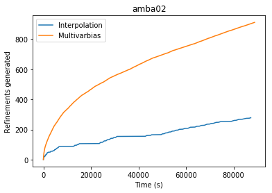
(a)

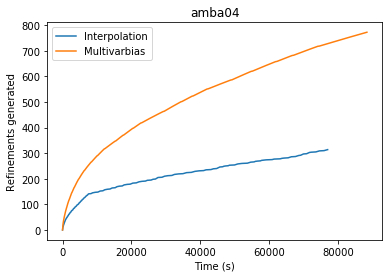
(b)

(c)

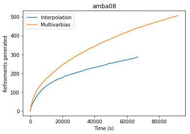
(d)

(e)

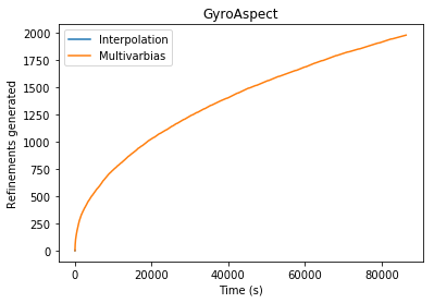
(f)

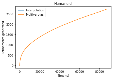
Figure 7: Total number of refinement nodes explored over time

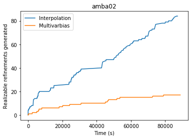
(a)

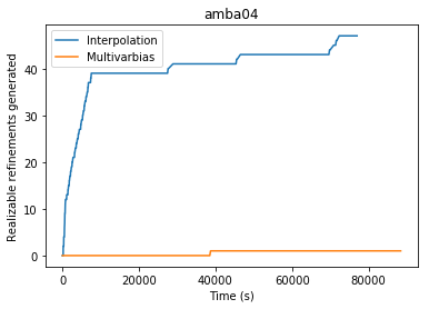
(b)

(c)

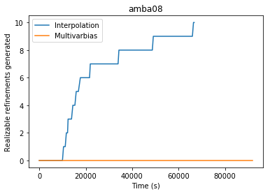
(d)

(e)

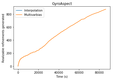
(f)

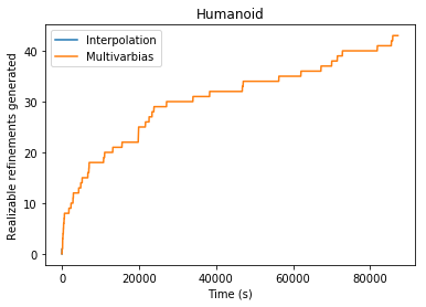
Figure 8: Number of realizable refinement nodes discovered over time (excluding vacuously realizable ones)

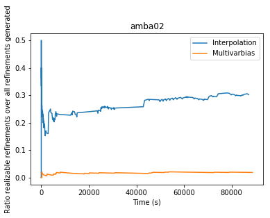
(a)

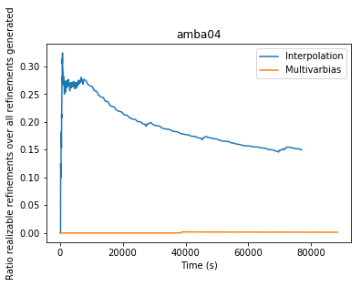
(b)

(c)

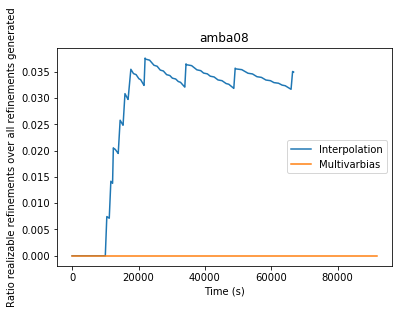
(d)

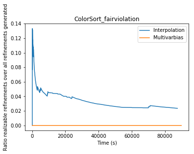
(e)

(f)

Figure 9: Ratio between realizable nodes and total generated nodes over time

Fig. 8 shows the number of realizable refinements discovered over time. In all case studies, the curve of interpolation remains above the one of multivarbias for the entire time frame where both approaches are executing. Therefore, it appears evident that interpolation is more focused on realizable nodes than multivarbias. This observation is corroborated by Fig. 9, which shows the proportion of realizable refinements discovered over all explored nodes over time. The interpolation approach settles around a value bigger than 15% in the first four case studies, while multivarbias remains close to 0%. In addition, the latter does not find any realizable refinement at all in the AMBA08 and ColorSort case studies.

On GyroAspect, interpolation explores 4 nodes, out of which it finds 2 solutions; on Humanoid, 3 nodes are explored, all of them being solutions to realizability; the total exploration time is less than 10 seconds. On the other hand, multivarbias finds 873 solutions on GyroAspect and 43 solutions on Humanoid by running throughout the entire 24-hour time frame. In both cases, the maximum ratio of realizable solutions over the total explored nodes is achieved by interpolation.

6.5 Discussion

A reason for the efficiency of interpolation can be sought in its addressing unrealizable cores directly. Given a GR(1) specification $\langle\phi^{\mathcal{E}},\phi^{\mathcal{S}}\rangle$ with unrealizable core $\phi^{uc}$, and a refinement $\psi$, we say that $\psi$ targets $\phi^{uc}$ if and only if the specification $\langle\phi^{\mathcal{E}}\cup\{\psi\},\phi^{uc}$ is realizable. Intuitively, any unrealizable core must be targeted by a refinement that solves the unrealizability problem. Therefore, when building the refinement tree it is desirable that at least an unrealizable core be targeted by a partial refinement.

Table 2 shows the percentage of nodes targeting their respective parent’s unrealizable core violated by the produced counterstrategy (see Section 2 for the relationship between counterstrategies and unrealizable cores). By comparing this with Fig. 9, notice that for each approach and each case study the procedure is most efficient in identifying realizable refinements if the proportion of nodes targeting their parent’s unrealizable core is higher on that case study.

Table 2: Percentage of nodes targeting parent’s unrealizable cores

	Interpolation	Multivarbias
AMBA02	88.17%	5.48%
AMBA04	100%	1.03%
AMBA08	100%	0.39%
ColorSort	45.09%	1.6%
GyroAspect	100%	80.5%
Humanoid	100%	100%

Therefore, producing refinements from interpolants (which in turn are computed from the translation of an unrealizable core), amounts to performing an educated choice of the variables to use in the refinements to be generated.

The larger number of solutions found by multivarbias in GyroAspect and Humanoid may be related to the size of the initial specification: the last two case studies are the smallest in terms of number of variables; therefore the space of possible choices for variables is small, and the likelihood of choosing a set of variables leading to a solution is higher. However, the number of variables alone may not be sufficient to characterize a class of problems where random variable selection works better than interpolation; in fact, AMBA02 has the same size in terms of number of variables, but in that case interpolation shows better performance than multivarbias.

The other difference to be considered lies in the number of initial assumptions and guarantees, which is higher in AMBA02 than in the other two case studies. This leads to longer translations from LTL to Boolean, which in turn potentially lead to longer interpolants and therefore more nodes in interpolation’s refinement tree. Therefore, in characterizing such class of problems the number of initial assumptions and guarantees plays a central role as well. Further studies are to be conducted in this direction.

7 Discussion

A direction of improvement of our approach lies in the selection of the counterrun to generate refinements from. Currently this choice is made at random, and only one counterrun is selected at every refinement synthesis step. Alternative approaches can be devised where more than one counterrun is selected, and/or computable heuristics of counterruns are exploited in order to focus on the ones with the largest number of alternative solutions. The use of heuristics would mitigate the effect of generating more intermediate nodes in the refinement tree that do not lead to realizable specifications.

Recently Justice Violations Transition Systems (JVTS) Kuvent et al (2017) have been proposed as alternatives to counterstrategies for debugging unrealizable specifications. The authors show that these structures are more concise and their computation is more time-efficient than counterstrategies, while retaining the same expressive power. However, to our knowledge no refinement approach has been proposed to date that uses such structures. In our work, we focus on counterstrategies in order to provide a fairer comparison with the state of the art. Investigation on how interpolation can be integrated with JVTSes is matter for future work. The use of JVTSes, however, by speeding up the counterstrategy generation phase, will allow to generate bigger refinement trees in a given time, possibly discovering a higher number of solutions.

8 Related Work

8.1 Revision of systems specifications

GR(1) assumptions refinement is an instance of the general problem of LTL specification revision. This has applications in many contexts, like robot motion planning Fainekos (2011); Kim et al (2015), operational requirements elaboration Alrajeh et al (2013).

The work in D’Ippolito et al (2014) takes a complementary perspective on GR(1) assumptions refinement by proposing a framework that weakens guarantees in order to adapt the functional behavior of a controller in accordance with observed violations of some given assumptions.

Other related work on assumption refinement includes those operating directly on game structures Chatterjee et al (2008). With regard to the parity game model used for controller synthesis (such as in Sohail and Somenzi (2013); Sohail et al (2008)), this paper defines the concept of safety assumptions as sets of edges that have to be avoided by the environment, and the concept of fairness assumptions as sets of edges that have to be traversed by the environment infinitely often. The work devises an algorithm for finding minimal edge sets in order to ensure that the controller has a winning strategy. Our approach instead focuses on synthesizing general declarative temporal assertions whose inclusion has the effect of removing edges from the game structure.

The problem of synthesizing environment constraints has been tackled in the context of assume-guarantee reasoning for compositional model checking Păsăreanu et al (1999); Cobleigh et al (2003); Gheorghiu Bobaru et al (2008) to support compositional verification. In these, assumptions are typically expressed as labeled transition systems (LTSs) and learning algorithms like ${\mathcal{L}}^{*}$ Angluin (1987) are used to incrementally refine the environment assumptions needed in order to verify the satisfaction of properties.

Add discussion here about abstraction refinement

Add discussion here Specification mining from execution traces

8.2 Oracle-Guided Inductive Synthesis

Countstrategy-guided assumptions refinement is an instance of the Oracle-Guided Inductive Synthesis (OGIS) framework Seshia (2015); Jha and Seshia (2017). This framework consists of an iterative interaction between a learner, which tries to learn some solution concept by induction over a set of examples, and an oracle, which answers the learner’s queries by providing meaningful examples for the learning process. In our context, the solution concept to learn is a refinement that makes a GR(1) specification realizable; the learner is the refinement synthesis procedure (Algorithm 2 described in Section 2.3); and the oracle is the realizability checking engine (invoked in line 1 of Algorithm 1). Other instances of OGIS are counterexample-guided inductive synthesis of programs Jha et al (2010); Alur et al (2013a); Jha and Seshia (2014) of abstraction refinement Clarke (2000); Esparza et al (2006) and obstacle detection Alrajeh et al (2012).

8.3 Applications of Craig interpolation

Craig interpolants have been deployed in the context of abstraction refinement for verification in Esparza et al (2006); D’Silva et al (2008). The differences with our work are in specification language and overall objective: they seek additional assertions for static analysis of programs, while we look for GR(1) refinements of systems specifications to enable their automated synthesis. The authors of Degiovanni et al (2014) use interpolation to support the extraction of pre- and trigger-conditions of operations within event-driven systems to enable the ‘satisfaction’ of goals expressed within restricted fragment of LTL. Though different in objective, approach and class of properties, our technique can help in identifying specifications operationalizable by Degiovanni et al (2014). This work also inspires our translation procedure from temporal logic to pure Boolean and vice versa.

9 Conclusions

We presented an interpolation-based approach for synthesizing weak environment assumptions for GR(1) specifications. Our approach exploits the information in counterstrategies and unrealizable cores to compute assumptions that directly target the cause of unrealizability. Compared to closely related approaches Alur et al (2013b); Li et al (2011), our algorithm does not require the user to provide the set of variables upon which the assumptions are constructed. The case study applications show that our approach implicitly performs a variable selection that targets an unrealizable core, allowing for a quicker convergence to a realizable specification.

The final set of refinements is influenced by the choice of counterplay. We are investigating in our current work the effect of and criteria over the counterplay selection particularly on the full-separability of interpolants. Furthermore, since interpolants are over-approximations of the counterplays, the final specification is an under-approximation. In future work, we will explore the use of witnesses (winning strategies for the system) to counteract this effect. Finally, the applicability of our approach depends on the separability properties of the computed interpolants: further investigation is needed to characterize the conditions under which an interpolation algorithm returns fully-separable interpolants.

References

- Alrajeh et al (2012) Alrajeh D, Kramer J, van Lamsweerde A, Russo A, Uchitel S (2012) Generating obstacle conditions for requirements completeness. In: ACM/IEEE 34th International Conference on Software Engineering, pp 705–715
- Alrajeh et al (2013) Alrajeh D, Kramer J, Russo A, Uchitel S (2013) Elaborating Requirements Using Model Checking and Inductive Learning. IEEE Transactions on Software Engineering 39(3):361–383
- Alur et al (2013a) Alur R, Bodik R, Juniwal G, Martin MMK, Raghothaman M, Seshia SA, Singh R, Solar-Lezama A, Torlak E, Udupa A (2013a) Syntax-guided synthesis. In: 2013 Formal Methods in Computer-Aided Design, pp 1–8
- Alur et al (2013b) Alur R, Moarref S, Topcu U (2013b) Counter-strategy guided refinement of GR(1) temporal logic specifications. In: Formal Methods in Computer-Aided Design, pp 26–33
- Alur et al (2015) Alur R, Moarref S, Topcu U (2015) Pattern-Based Refinement of Assume-Guarantee Specifications in Reactive Synthesis. In: 21st International Conference on Tools and Algorithms for the Construction and Analysis of Systems, pp 501–516
- Angluin (1987) Angluin D (1987) Learning regular sets from queries and counterexamples. Information and Computation 75(2):87–106, DOI 10.1016/0890-5401(87)90052-6
- Beer et al (2001) Beer I, Ben-David S, Eisner C, Rodeh Y (2001) Efficient detection of vacuity in temporal model checking. Formal Methods in System Design 18(2):141–163
- Biere et al (2003) Biere A, Cimatti A, Clarke EM, Strichman O, Zhu Y (2003) Bounded Model Checking. Advances in Computers 58
- Bloem et al (2010) Bloem R, Cimatti A, Greimel K, Hofferek G, Könighofer R, Roveri M, Schuppan V, Seeber R (2010) RATSY – A New Requirements Analysis Tool with Synthesis. In: 22nd International Conference on Computer Aided Verification, pp 425–429
- Bloem et al (2012) Bloem R, Jobstmann B, Piterman N, Pnueli A, Sa’Ar Y (2012) Synthesis of Reactive(1) designs. Journal of Computer and System Sciences 78(3):911–938
- Bruttomesso et al (2008) Bruttomesso R, Cimatti A, Franzén A, Griggio A, Sebastiani R (2008) The MATHSAT 4 SMT solver: Tool paper. In: 20th International Conference on Computer Aided Verification, pp 299–303
- Cavezza and Alrajeh (2017) Cavezza DG, Alrajeh D (2017) Interpolation-Based GR(1) Assumptions Refinement. In: Tools and Algorithms for the Construction and Analysis of Systems, Springer Berlin Heidelberg, pp 281–297
- Chatterjee et al (2008) Chatterjee K, Henzinger TA, Jobstmann B (2008) Environment Assumptions for Synthesis. In: 9th International Conference on Concurrency Theory, pp 147–161
- Cimatti et al (2008a) Cimatti A, Griggio A, Sebastiani R (2008a) Efficient Interpolant Generation in Satisfiability Modulo Theories. In: 14th International Conference on Tools and Algorithms for the Construction and Analysis of Systems, pp 397–412
- Cimatti et al (2008b) Cimatti A, Roveri M, Schuppan V, Tchaltsev A (2008b) Diagnostic Information for Realizability. In: 9th International Conference on Verification, Model Checking, and Abstract Interpretation, pp 52–67
- Clarke (2000) Clarke E (2000) Counterexample-guided abstraction refinement. In: 10th International Symposium on Temporal Representation and Reasoning, pp 7–8
- Cobleigh et al (2003) Cobleigh JM, Giannakopoulou D, Păsăreanu CS (2003) Learning Assumptions for Compositional Verification. In: 9th International Conference Tools and Algorithms for the Construction and Analysis of Systems, pp 331–346
- Craig (1957) Craig W (1957) Three uses of the Herbrand-Gentzen theorem in relating model theory and proof theory. The Journal of Symbolic Logic 22(03):269–285
- Degiovanni et al (2014) Degiovanni R, Alrajeh D, Aguirre N, Uchitel S (2014) Automated goal operationalisation based on interpolation and SAT solving. In: ACM/IEEE 36th International Conference on Software Engineering, pp 129–139
- D’Ippolito et al (2014) D’Ippolito N, Braberman V, Kramer J, Magee J, Sykes D, Uchitel S (2014) Hope for the Best, Prepare for the Worst: Multi-tier Control for Adaptive Systems. Proceedings of the 36th International Conference on Software Engineering pp 688–699
- D’Silva et al (2008) D’Silva V, Kroening D, Weissenbacher G (2008) A Survey of Automated Techniques for Formal Software Verification. IEEE Transactions on Computer-Aided Design of Integrated Circuits and Systems 27(7):1165–1178
- Esparza et al (2006) Esparza J, Kiefer S, Schwoon S (2006) Abstraction Refinement with Craig Interpolation and Symbolic Pushdown Systems. In: 12th International Conference on Tools and Algorithms for the Construction and Analysis of Systems, pp 489–503
- Fainekos (2011) Fainekos GE (2011) Revising temporal logic specifications for motion planning. Proceedings - IEEE International Conference on Robotics and Automation pp 40–45, DOI 10.1109/ICRA.2011.5979895
- Gheerbrant and ten Cate (2009) Gheerbrant A, ten Cate B (2009) Craig Interpolation for Linear Temporal Languages. In: 23rd International Workshop on Computer Science Logic, pp 287–301
- Gheorghiu Bobaru et al (2008) Gheorghiu Bobaru M, Păsăreanu CS, Giannakopoulou D (2008) Automated Assume-Guarantee Reasoning by Abstraction Refinement. In: 20th International Conference Computer Aided Verification, pp 135–148
- Jha and Seshia (2014) Jha S, Seshia SA (2014) Are there good mistakes? A theoretical analysis of CEGIS. In: 3rd Workshop on Synthesis, pp 84–99
- Jha and Seshia (2017) Jha S, Seshia SA (2017) A theory of formal synthesis via inductive learning. Acta Informatica 54(7):693–726, DOI 10.1007/s00236-017-0294-5
- Jha et al (2010) Jha S, Gulwani S, Seshia SA, Tiwari A (2010) Oracle-guided component-based program synthesis. ACM/IEEE 32nd International Conference on Software Engineering pp 215–224
- Kamide (2015) Kamide N (2015) Interpolation theorems for some variants of LTL. Reports on Mathematical Logic 50:3–30
- Kim et al (2015) Kim K, Fainekos G, Sankaranarayanan S (2015) On the minimal revision problem of specification automata. International Journal of Robotics Research 34(12):1515–1535, DOI 10.1177/0278364915587034
- Könighofer et al (2009) Könighofer R, Hofferek G, Bloem R (2009) Debugging formal specifications using simple counterstrategies. In: Formal Methods in Computer-Aided Design, pp 152–159
- Krajíček (1997) Krajíček J (1997) Interpolation theorems, lower bounds for proof systems, and independence results for bounded arithmetic. The Journal of Symbolic Logic 62(02):457–486
- Kuvent et al (2017) Kuvent A, Maoz S, Ringert JO (2017) A symbolic justice violations transition system for unrealizable GR(1) specifications. In: Proceedings of the 2017 11th Joint Meeting on Foundations of Software Engineering - ESEC/FSE 2017, ACM Press, 1, pp 362–372
- van Lamsweerde (2009) van Lamsweerde A (2009) Requirements Engineering - From System Goals to UML Models to Software Specifications. Wiley
- van Lamsweerde and Letier (2000) van Lamsweerde A, Letier E (2000) Handling obstacles in goal-oriented requirements engineering. IEEE Trans Software Eng 26(10):978–1005
- Li et al (2011) Li W, Dworkin L, Seshia SA (2011) Mining assumptions for synthesis. In: ACM/IEEE 9th International Conference on Formal Methods and Models for Codesign, pp 43–50
- Li et al (2014) Li W, Sadigh D, Sastry SS, Seshia SA (2014) Synthesis for human-in-the-loop control systems. In: 20th International Conference on Tools and Algorithms for the Construction and Analysis of Systems, pp 470–484
- Löding et al (2016) Löding C, Madhusudan P, Neider D (2016) Abstract Learning Frameworks for Synthesis. In: Tools and Algorithms for the Construction and Analysis of Systems: 22nd International Conference, TACAS 2016 held as part of the european joint conferences on theory and practice of software, ETAPS 2016 Eindhoven, The Netherlands, April 2-8, 2016, Proceed, Springer Berlin Heidelberg, vol 9636, pp 167–185
- Manna and Pnueli (1992) Manna Z, Pnueli A (1992) The Temporal Logic of Reactive and Concurrent Systems. Springer
- McMillan (2003) McMillan KL (2003) Interpolation and SAT-Based Model Checking. In: 15th International Conference on Computer Aided Verification, pp 1–13
- Pnueli and Rosner (1989) Pnueli A, Rosner R (1989) On the synthesis of a reactive module. In: Proceedings of the 16th ACM SIGPLAN-SIGACT symposium on Principles of programming languages - POPL ’89, ACM Press, JANUARY 1989, pp 179–190
- Păsăreanu et al (1999) Păsăreanu C, Dwyer M, Huth M (1999) Assume-guarantee model checking of software: A comparative case study. Theoretical and Practical Aspects of SPIN Model Checking pp 168–183
- Seshia (2015) Seshia SA (2015) Combining Induction, Deduction, and Structure for Verification and Synthesis. IEEE 103(11):2036–2051
- Sohail and Somenzi (2013) Sohail S, Somenzi F (2013) Safety first: a two-stage algorithm for the synthesis of reactive systems. International Journal on Software Tools for Technology Transfer 15(5-6):433–454
- Sohail et al (2008) Sohail S, Somenzi F, Ravi K (2008) A Hybrid Algorithm for LTL Games. In: Verification, Model Checking, and Abstract Interpretation, pp 309–323