Infinite Variational Autoencoder for Semi-Supervised Learning

Abstract

This paper presents an infinite variational autoencoder (VAE) whose capacity adapts to suit the input data. This is achieved using a mixture model where the mixing coefficients are modeled by a Dirichlet process, allowing us to integrate over the coefficients when performing inference. Critically, this then allows us to automatically vary the number of autoencoders in the mixture based on the data. Experiments show the flexibility of our method, particularly for semi-supervised learning, where only a small number of training samples are available.

1 Introduction

The Variational Autoencoder (VAE) [18] is a newly introduced tool for unsupervised learning of a distribution $p(\mathbf{x})$ from which a set of training samples $\mathbf{x}$ is drawn. It learns the parameters of a generative model, based on sampling from a latent variable space $\mathbf{z}$, and approximating the distribution $p(\mathbf{x}|\mathbf{z})$. By designing the latent space to be easy to sample from (e.g. Gaussian) and choosing a flexible generative model (e.g. a deep belief network) a VAE can provide a flexible and efficient means of generative modeling.

One limitation of this model is that the dimension of the latent space and the number of parameters in the generative model are fixed in advance. This means that while the model parameters can be optimized for the training data, the capacity of the model must be chosen a priori, assuming some foreknowledge of the training data characteristics.

In this paper we present an approach that utilizes Bayesian non-parametric models [1, 8, 31, 13] to produce an infinite mixture of autoencoders. This infinite mixture is capable of growing with the complexity of the data to best capture its intrinsic structure.

Our motivation for this work is the task of semi-supervised learning. In this setting, we have a large volume of unlabelled data but only a small number of labelled training examples. In our approach, we train a generative model using unlabelled data, and then use this model combined with whatever labelled data is available to train a discriminative model for classification.

We demonstrate that our infinite VAE outperforms both the classical VAE and standard classification methods, particularly when the number of available labelled samples is small. This is because the infinite VAE is able to more accurately capture the distribution of the unlabelled data. It therefore provides a generative model that allows the discriminative model, which is trained based on its output, to be more effectively learnt using a small number of samples.

The main contribution of this paper is twofold: (1) we provide a Bayesian non-parametric model for combining autoencoders, in particular variational autoencoders. This bridges the gap between non-parametric Bayesian methods and the deep neural networks; (2) we provide a semi-supervised learning approach that utilizes the infinite mixture of autoencoders learned by our model for prediction with from a small number of labeled examples.

The rest of the paper is organized as follows. In Section 2 we review relevant methods, while in Section 3 we briefly provide background on the variational autoencoder. In Section 4 our non-parametric Bayesian approach to infinite mixture of VAEs is introduced. We provide the mathematical formulation of the problem and how the combination of Gibbs sampling and Variational inference can be used for efficient learning of the underlying structure of the input. Subsequently in Section 5, we combine the infinite mixture of VAEs as an unsupervised generative approach with discriminative deep models to perform prediction in a semi-supervised setting. In Section 6 we provide empirical evaluation of our approach on various datasets including natural images and 3D shapes. We use various discriminative models including Residual Network [12] in combination with our model and show our approach is capable of outperforming our baselines.

2 Related Work

Most of the successful learning algorithms, specially with deep learning, require large volume of labeled instance for training. Semi-supervised learning seeks to utilize the unlabeled data to achieve strong generalization by exploiting small labeled examples. For instance unlabeled data from the web is used with label propagation in [6] for classification. Similarly, semi supervised learning for object detection in videos [28] or images [43, 7].

Most of these approaches are developed by either (a) performing a projection of the unlabeled and labeled instances to an embedding space and using nearest neighbors to utilize the distances to infer the labeled similar to label propagation in shallow [15, 42, 14] or deep networks [45]; or (b), formulating some variation of a joint generative-discriminative model that uses the latent structure of the unlabeled data to better learn the decision function with labeled instances. For example ensemble methods [3, 26, 24, 47, 5] assigns pseudo-class labels based on the constructed ensemble learner and in turn uses them to find a new proper learner to be added to the ensemble.

In recent years, deep generative models have gained attention with success in Restricted Boltzman machines (and its infinite variation [4]) and autoencoders (e.g. [17, 21]) with their stacked variation [41]. The representations learned from these unsupervised approaches are used for supervised learning.

Other related approaches to ours are adversarial networks [9, 29, 25] in which the generative and discriminative model are trained jointly. This model penalizes the generative model for as long as the samples drawn from it does not perform well in the discriminative model in a min-max optimization. Although theoretically well justified, training such models proved to be difficult.

Our formulation for semi-supervised learning is also related to the Highway [40] and Memory [44] networks that seek to combine multiple channels of information that capture various aspects of the data for better prediction, even though their approaches mainly focus on depth.

3 Variational autoencoder

While typically autoencoders assume a deterministic latent space, in a variational autoencoder the latent variable is stochastic. The input $\mathbf{x}$ is generated from a variable in that latent space $\mathbf{z}$. Since the joint distribution of the input when all the latent variables are integrated out is intractable, we resort to a variational inference (hence the name). The model is defined as:

$$p_{\boldsymbol{\theta}}(\mathbf{z}) = \mathcal{N}(\mathbf{z};0,\mathbf{I}),$$

$$p_{\boldsymbol{\theta}}(\mathbf{x}|\mathbf{z}) = \mathcal{N}(\mathbf{x};\mu(\mathbf{z}),\sigma(\mathbf{z})\mathbf{I}),$$

$$q_{\phi}(\mathbf{z}|\mathbf{x}) = \mathcal{N}(\mathbf{x};\mu(\mathbf{x}),\sigma(\mathbf{x})\mathbf{I}),$$

where $\boldsymbol{\theta}$ and $\boldsymbol{\phi}$ are the parameters of the model to be found. The objective is then to minimize the following loss,

$$-\underbrace{\mathbb{E}_{\mathbf{z}\sim q(\mathbf{z}|\mathbf{x})}\left[\log p(\mathbf{x}|\mathbf{z})\right]}_{\text{reconstruction error}}+\underbrace{\text{KL}\left(q_{\phi}(\mathbf{z}|\mathbf{x})||p(\mathbf{z})\right)}_{\text{regularization}}.$$ (1)

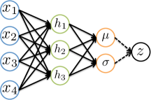
Figure 1: Variational encoder: the solid lines are direct connection and dotted lines are sampled. The input layer represented by $\mathbf{x}$ and the hidden layer $\mathbf{h}$ determine moments of the variational distribution. From the variational distribution the latent variable $\mathbf{z}$ is sampled.

The first term in this loss is the reconstruction error, or expected negative log-likelihood of the datapoint. The expectation is taken with respect to the encoder’s distribution over the representations by taking a few samples. This term encourages the decoder to learn to reconstruct the data when using samples from the latent distribution. A large error indicates the decoder is unable to reconstruct the data. A schematic network of the encoder is shown in Figure 1. As shown, deep network learns the mean and variance of a Gaussian from which subsequent samples of $\mathbf{z}$ are generated.

The second term is the Kullback-Leibler divergence between the encoder’s distribution $q_{\theta}(\mathbf{z}|\mathbf{x})$ and $p(\mathbf{z})$. This divergence measures how much information is lost when using $q$ to represent a prior over $\mathbf{z}$ and encourages its values to be Gaussian. To perform inference efficiently a reparameterization trick is employed [18] that in combination with the deep neural networks allow for the model to be trained with the backpropagation.

4 Infinite Mixture of Variational autoencoder

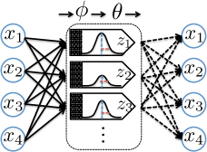
Figure 2: Infinite mixture of variational inference is shown as a block within which VAE components operate. Each latent variable $z_{i}$ (one dimensional in this illustration) in each VAE is drawn from a Gaussian distribution. Solid lines indicate nonlinear encoding and the dashed lines are decoders. In this diagram, $\boldsymbol{\phi}$ and $\boldsymbol{\theta}$ are the parameters of the encoder and decoder respectively.

An auto encoder in its classical form seeks to find an embedding of the input such that its reproduction has the least discrepancy. A variational autoencoder modifies this notion by introducing a non-parametric Bayesian view where the conditional distribution of the latent variables, given the input, is similar to the distribution of the input given the latent variable, while ensuring the distribution of the latent variable is close to a Gaussian with zero mean and variance one.

A single variational encoder has a fixed capacity and thus might not be able to capture the complexity of the input well. However by using a collection of VAEs, we can ensure that we are able to model the data, by adapting the number of VAEs in the collection to fit the data. In our infinite mixture, we seek to find a mixture of these variational autoencoders such that its capacity can theoretically grow to infinity. Each autoencoder then is able to capture a particular aspect of the data. For instance, one might be better at representing round structures, and another better at straight lines. This mixture intuitively represents the various underlying aspects of the data. Moreover, since each VAE models the uncertainty of its representations through the density of the latent variable, we know how confident each autoencoder is in reconstructing the input.

One advantage of our non-parametric mixture model is that we are taking a Bayesian approach in which the distribution of the parameters are taken into account. As such, we capture the uncertainty of the model parameters. The autoencoders that are less confident about their reconstruction, have less effect on the output. As shown in Figure 2, each encoder finds a distribution for the embedding variable with some probability through a nonlinear transform (convolution or fully connected layers in neural net). Each autoencoder in the mixture block produces a probability measure for its ability to reconstruct the input. This behavior has parallels to the brain’s ability to develop specialized regions responsible for particular visual tasks and processing particular types of image pattern.

Mixture models are traditionally built using a pre-determined number of weighted components. Each weight coefficient determines how likely it is for a predictor to be successful in producing an accurate output. These coefficients are drawn from a multinomial distribution where the number of these coefficients are fixed. On the other hand, to learn an infinite mixture of the variational autoencoders in a non-parametric Bayesian manner we employ Dirichlet process. In Dirichlet process, unlike traditional mixture models, we assume the probability of each component is drawn from a multinomial with a Dirichlet prior. The advantage of taking this approach is that we can integrate over all possible mixing coefficients. This allows for the number of components to be determined based on the data.

Initalize VAE assignments $\mathbf{c}$

$A_{c}=\{\}$ $\quad\forall c=1,\ldots,C$

while not converged do

     for $\mathbf{x}_{i}\in X$ do $\triangleright$ VAE assignments

         Assign $\mathbf{c}_{i}^{\text{new}}$ to new VAE according to Eq. 3

         Otherwise, sample $\mathbf{c}_{i}^{\text{new}}$ according to Eq. 2

         if $\mathbf{c}_{i}^{\text{new}}\neq\mathbf{c}_{i}$ then

              $A_{\mathbf{c}_{i}}=A_{\mathbf{c}_{i}}\cup\{i\}$ $\triangleright$ Given VAE has to forget

         end if

     end for

     Update $C$ for new VAEs

     for $c=1,\ldots,C$ do $\triangleright$ Update VAEs

         Forget $A_{c}$ in $c$th VAE

         Learn $c$th VAE $\quad\forall i$ where $\mathbf{c}_{i}^{\text{new}}=c$

     end for

end while

Return Infinite Mixture of VAEs

Algorithm 1 Learning Infinite mixture of Variational autoencoders

Formally, let $\mathbf{c}$ be the assignment matrix for each instance to a VAE component (that is, which VAE is able to best reconstruct instance $i$) and $\boldsymbol{\pi}$ be the mixing coefficient prior for $\mathbf{c}$. For $n$ unlabeled instances we model the infinite mixture of VAEs as,

$$p(\mathbf{c},\boldsymbol{\pi},\boldsymbol{\theta},\mathbf{x}_{1,\ldots,n},\alpha)\!\!\!\! = \!\!\!\!p(\mathbf{c}|\boldsymbol{\pi})p(\boldsymbol{\pi}|\alpha)\int p_{\boldsymbol{\theta}}(\mathbf{x}_{1,\ldots,n}|\mathbf{c},\mathbf{z})p(\mathbf{z})d\mathbf{z}$$

We assume the mixing coefficients are drawn from a Dirichlet distribution with parameter $\alpha$ (see Figure 3 for examples),

$$p(\pi_{1},\ldots,\pi_{C}|\alpha) \sim \text{Dir}(\alpha/C),$$

To determine the membership of each instance in one of the components of the mixture model, i.e. the likelihood that each variational autoencoder is able to encode the input and reconstruct it with minimum loss, we compute the conditional probability of membership. This conditional probability of each instance belonging to an autoencoder component is computed by integrating over all mixing components $\boldsymbol{\pi}$, that is [35, 36],

$$p(\mathbf{c},\boldsymbol{\theta},\mathbf{x}_{1,\ldots,n},\alpha)\!\!\!\!\!\! = \!\!\!\!\!\!\int\!\!\int\prod_{i}^{n}p{}_{\boldsymbol{\theta}_{\mathbf{c}_{i}}}(\mathbf{x}_{i}|\mathbf{z}_{\mathbf{c}_{i}})p(\mathbf{z}_{\mathbf{c}_{i}})p(\mathbf{c}|\boldsymbol{\pi})p(\boldsymbol{\pi}|\alpha)d\boldsymbol{\pi}d\mathbf{z}_{\mathbf{c}_{i}}$$

This integration accounts for all possible membership coefficients for all the assignments of the instances to VAEs. The distribution of $\mathbf{c}$ is multinomial, for which the Dirichlet distribution is its conjugate prior, and as such this integration is tractable. To perform inference for the parameters $\boldsymbol{\theta}$ and $\mathbf{c}$ we perform block Gibbs sampling, iterating between optimizing for $\boldsymbol{\theta}$ for each VAE and updating the assignments in $\mathbf{c}$. Optimization uses the variational autoencoder’s trick by minimizing the loss in Equation 6. To update $\mathbf{c}$, we perform the following Gibbs sampling:

• The conditional probability that an instance $i$ belongs to VAE $c$:

  $$p(\mathbf{c}_{i}=c|\mathbf{c}_{{\backslash}i},\mathbf{x}_{i},\alpha) = \frac{\eta_{c}(\mathbf{x}_{i})}{n-1+\alpha}$$ (2)

  where $\eta_{c}(\mathbf{x}_{i})$ is the occupation number of cluster $c$, excluding instance $i$ for $n$ instances. We define,

  $$\eta_{c}(\mathbf{x}_{i}) = (n-1)p_{\boldsymbol{\theta}_{c}}(\mathbf{c}_{i}=c|\mathbf{x}_{i}),$$

  and

  $$p_{\boldsymbol{\theta}_{c}}(\mathbf{c}_{i}=c|\mathbf{x}_{i})\!\!\!\!\! =\!\!\!\!\! \frac{\exp\left(\mathbb{E}_{\mathbf{z}_{c}\sim q_{\phi_{c}(\mathbf{z}|\mathbf{x})}}\left[\log p_{\boldsymbol{\theta}_{c}}(\mathbf{x}_{i}|\mathbf{z}_{c})\right]\right)}{\sum_{j}\exp\left(\mathbb{E}_{\mathbf{z}_{j}\sim q_{\phi_{j}(\mathbf{z}|\mathbf{x})}}\left[\log p_{\boldsymbol{\theta}_{j}}(\mathbf{x}_{i}|\mathbf{z}_{j})\right]\right)}$$

  which in evaluates how likely an instance $\mathbf{x}_{i}$ is to be assigned to the $c$th VAE using latent samples $\mathbf{z}_{c}$.

• The probability that instance $i$ is not well represented by any of the existing autoencoders and a new encoder has to be generated:

$$p(\mathbf{c}_{i}=c|\mathbf{c}_{{\backslash}i},\mathbf{x}_{i},\alpha) = \frac{\alpha}{n-1+\alpha}.$$ (3)

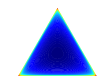
(a) $\alpha=0.99$

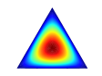
(b) $\alpha=2$

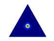
(c) $\alpha=50$

Figure 3: Dirichlet distribution with various values of $\alpha$. Smaller values of $\alpha$ tend to concentrate the mass in the corners (in this simplex example and in general as the dimensions increase). These smaller values reduce the chance of generating new autoencoder components.

Note that in principle, $\eta_{c}(\mathbf{x}_{i})$ is the a measure calculated by excluding the $i$th instance in the observations so that its membership is calculated with respect to its ”similarity” to other members of the cluster. However, here we use $c$th VAE as an estimate of this occupation number for performance reasons. This is justified so long as the influence of a single observation on the latent representation of an encoder is negligible. In Equation 2 when a sample for the new assignment is drawn from this multinomial distribution there is a chance for completely different VAE to fit this new instance. If the new VAE is not successful in fitting, the instance will be assigned to its original VAE with high probability in the subsequent iteration.

The entire learning process is summarised in Algorithm 1. To improve performance, at each iteration of our approach, we keep track of the $c$th VAE assignment changes in a set $A_{c}$. This allows us to efficiently update each VAE using a backpropagation operation for the new assignments. We perform two operations after VAE assignments are done: (1) forget, and (2) learn. In forgetting stage, we tend to unlearn the instances that were assigned to the given VAE. It is done by performing a gradient update with negative learning-rate, i.e. reverse backpropagation. In the learning stage on the other hand, we update the parameters of the given VAE with positive learning-rate, as is commonly done using backpropagation. This alternation allows for structurally similar instances that can share latent variables to be learned with a single VAE, while forgetting those that are not well suited.

To reconstruct an input $\mathbf{x}$ with an infinite mixture, the expected reconstruction is defined as:

$$\mathbb{E}[\mathbf{x}]=\sum_{c}p_{\boldsymbol{\theta}_{c}}(\mathbf{c}_{i}=c|\mathbf{x}_{i})\mathbb{E}_{q_{\phi}(\mathbf{z}_{c}|\mathbf{x})}\left[\mathbf{x}|\mathbf{z}_{c}\right].$$ (4)

That is, we use each VAE to reconstruct the input and weight it with the probability of that VAE (this probability is inversely proportionate to the variance of each VAE).

5 Semi-Supervised Learning using Infinite autoencoders

Many of deep neural networks’ greatest successes have been in supervised learning, which depends on the availability of large labeled datasets. However, in many problems such datasets are unavailable and alternative approaches, such as combination of generative and discriminative models, have to be employed. In semi-supervised learning, where the number of labeled instances is small, we employ our infinite mixture of VAEs to assist supervised learning. Inspired by the mixture of experts [30, Chapter 11] we formulate the problem of predicting output $y^{*}$ for the test example $\mathbf{x}^{*}$ as,

$$p(y^{*}|\mathbf{x}^{*}) = \sum_{c}^{C}\underbrace{p(y^{*}|\mathbf{x}^{*},\boldsymbol{\omega}_{c})}_{\text{deep discriminative}}\times\,\,\underbrace{p_{\boldsymbol{\theta}_{c}}(\mathbf{c}_{i}=c|\mathbf{x}_{i})}_{\text{deep generative}}.$$

This formulation for prediction combines the discriminative power of a deep learner with parameter set $\boldsymbol{\omega}_{c}$, and a flexible generative model. For a given test instance $\mathbf{x}^{*}$, each discriminative expert produces a tentative output that is then weighted by the generative model. As such, each discriminative expert learns to perform better with instances that are more structurally similar from the generative model’s perspective.

During training we minimize the negative log of the discriminative term (log loss) weighted by the generative weight. Each instance’s weight–as calculated by the infinite autoencoder–acts as an additional coefficient for the gradient in the backpropagation. It leads to similar instances getting stronger weights in the neural net during training. Moreover, it should be noted that the generative and discriminative models can share deep parameters $\boldsymbol{\omega}_{c}$ and $\boldsymbol{\theta}_{c}$ at some level. In particular in our implementation, we only consider parameters of the last layer to be distinct for each discriminative and generative component. We summarize our framework in Figure 4.

While combining an unsupervised generative model and a supervised discriminative models is not itself novel, in our problem the generative model can grow to capture the complexity of the data. In addition, since we share the parameters of the discriminative and generative models, each unsupervised learner does not need to learn all the aspects of the input. In fact, in many classification problems with images, each pixel value hardly matters in the final decision. As such, by sharing parameters unsupervised model incurs a heavier loss when the distribution of the latent variables does not encourage the correct final decision. This sharing is done by reusing the parameters that are initialized with labels.

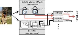
Figure 4: Our framework for infinite mixture of VAEs and semi-supervised learning. We share the parameters of the discriminative model at the lower levels for more efficient training and prediction. For each VAE in the mixture we have an expert (e.g. softmax) before the output. Thicker arrows indicate more probable connection.

6 Experiments

In this section, we examine the performance of our approach for semi-supervised classification on various datasets. We investigate how the combination of the generative and discriminative networks is able to perform semi-supervised learning effectively. Since convergence of Gibbs sampling can be very slow we first pre-train the base VAE with all the unlabeled examples. Each autoencoder is trained with a two dimensional latent variable $\mathbf{z}$ and initialized randomly. Hence each new VAE is already capable of reconstructing the input to a certain extent. During the sampling steps, this VAE becomes more specialized in a particular structure of the inputs. To further facilitate sampling, we set the number of clusters equal to the number of classes and use $100$ random labeled examples to fine-tune VAE assignments. At each iteration, if there is no instance assigned to a VAE, it will be removed. As such, the mixture grows and shrinks with each iteration as instances are assigned to VAEs. We report the results over 3 trials.

For comparing the autoencoder’s ability to internally capture the structure of the input, we compared latent representation obtained by a single VAE and the expected latent representation from our approach in Equation 4 and subsequently trained a support vector machine (SVM) with it. For computing expectations, we used $20$ samples from the latent variable space.

Once the generative model is learned with all the unlabelled instances using the infinite mixture model in Section 4, we randomly select a subset of labeled instances for training the discriminative model. Throughout the experiments, we share the parameters in the discriminative architecture from the input to the last layer so that each expert is represented by a softmax.

We report classification results in various problems including handwritten binary images, natural images and 3D shapes. Although the performance of our semi-supervised learning approach depends on the choice of the discriminative model, we observe our approach outperforms baselines particularly with smaller labeled instances. For all trainings–either discriminative or generative–we set the maximum number of iterations to $1000$ with batch size $500$ for the stochastic gradient descent with constant learning rate $0.001$. For VAEs we use the Adam [16] updates with $\beta_{1}=0.9$, $\beta_{2}$$=0.999$. However, we set a threshold on the changes in the loss to detect convergence and stop the training. Except for the binary images where we use a binary decoder ($p_{\boldsymbol{\theta}}(\mathbf{x}|\mathbf{z})$ is binomial), our decoder is continuous (($p_{\boldsymbol{\theta}}(\mathbf{x}|\mathbf{z})$ is Gaussian) in which samples from the latent space is used to regenerate the input to compute the loss.

In problems when the input is too complex for the autoencoder to perform well, we share the output of the last layer of the discriminative model with the VAEs.

6.1 MNIST Dataset

(a) Original Images

(b) VAE reconstruction (number of hidden variables $50$)

(c) VAE reconstruction (number of hidden variables $1024$)

(d) Infinite Mixture reconstruction (number of clusters $18$ using base VAE with number of hidden variables $50$)

Figure 5: An illustration of the autoencoder’s input reconstruction. First row is the original images. Reconstructions in Figure 5(b) and 5(c) are obtained from using a single VAE. Images in the last row are obtained from the proposed mixture model of $18$ VAEs each with $50$ hidden units. As seen, reconstructed images are clearer in Figure 5(d).

MNIST dataset contains $60,000$ training and $10,000$ test images of size $28\times 28$ of handwritten digits. Some random images from this dataset are shown in Figure 5(a). We use original VAE algorithm (single VAE) with $100$ iteration and $50$ hidden variables to learn a representation for these digits with binary distribution for the input $p_{\boldsymbol{\theta}}(\mathbf{x}|\mathbf{z})$. As shown in Figure 5(b), these reconstructions are very unclear and at times wrong (6th column where $7$ is wrongly reconstructed as $9$). Using this VAE as base, we train an infinite mixture of our generative model. After $10$ iterations with $\alpha=2$, the expected reconstruction $\mathbb{E}\left[\mathbf{x}\right]$ is depicted in Figure 5(d). We use 2 samples to compute $\mathbb{E}[\mathbf{x}]$ for $c$th VAE. As observed, this reconstruction is visually better and the mistake in the 6th column is fixed. Further, Figure 5(c) shows using VAE with $1024$ hidden units. It is interesting to note that even though our proposed model has smaller number of hidden units ($900$ vs $1024$), the reconstruction is better using our model.

In Table 1 we summarize reconstruction error (that is, $\|\mathbf{x}-\mathbb{E}\left[\mathbf{x}\right]\|$) for using our approach versus the original VAE. As seen, our approach performs similarly with the VAE when the number of hidden units are almost similar ($1000$ vs $1024$). As seen, with higher number of VAEs, we are able to reduce the reconstruction error significantly.

Method	$C$	# hidden units	Error
Infinite Mixture	2	100	$9.17$
	10	100	$5.12$
	17	100	$4.9$
VAE	1	100	$5.92$
	1	1024	$5.1$

Table 1: Reconstruction error for MNIST dataset as the norm of the difference of the input image and the expected reconstruction comparing our approach with the original VAE.

To test our approach in a semi-supervised setting, we use a deep Convolutional Neural Net (CNN). Our deep CNN architecture consists of two convolutional layers with $32$ filters of $5\times 5$ and Rectified Linear Unit (ReLU) activation and max-pooling of $2\times 2$ after each one. We added a fully connected layer with $256$ hidden units followed by a dropout layer and then the softmax output layer. As shown in Table 2, our infinite mixture with $17$ base VAEs has been able to outperform most of the state-of-the-art methods. Only recently proposed Virtual Adversarial Network [29] performs better than ours with small training examples.

Method/Labels	100	1000	All
Pseudo-label [23]	$10.49$	$3.64$	$0.81$
EmbedNN [45]	$16.9$	$5.73$	$3.59$
DGN [17]	$3.33\pm 0.14$	$2.40\pm 0.02$	$0.96$
Adversarial [9]			$0.78$
Virtual Adversarial [29]	$2.66$	$1.50$	$0.64\pm 0.03$
AtlasRBF [32]	$8.10\pm 0.95$	$3.68\pm 0.12$	$1.31$
PEA [2]	$5.21$	$2.64$	$2.30$
$\Gamma\text{-Model}$ [34]	$4.34\pm 2.31$	$1.71\pm 0.07$	$0.79\pm 0.05$
Baseline CNN	$8.62\pm 1.87$	$4.16\pm 0.35$	$0.68\pm 0.02$
Infinite Mixture	$3.93\pm 0.5$	$2.29\pm 0.2$	$0.6\pm 0.02$

Table 2: Test error for MNIST with 17 clusters and 100 hidden variables. Only [29] reports better performance than ours

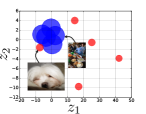
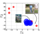
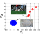
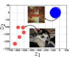
Figure 6: Two dimensional latent space found from training our infinite mixture of VAEs on Dogs dataset. We randomly selected 5 dog images and 5 images of anything else and plotted their latent representation in each VAE ($z_{1}$ for the first dimension and $z_{2}$ for the second one). The position of each circle represents the mean of the density for the given image in this space and its radius is the variance ($\mu$ and $\sigma$ in Figure 6, respectively). As shown, representation of non-dogs (blue circles) are generally clustered far away from the dogs (red circles). Moreover, dogs have smaller variance than non-dogs, hence the VAEs are uncertain about the representation of images that were not seen during training.

Method/Labels	100	1000	4000	All
AlexNet [20]	$69.59\pm 3.21$	$86.72\pm 0.66$	$89.88\pm 0.03$	$90.26\pm 0.25$
Infinite Mixture	$75.81\pm 1.83$	$89.28\pm 0.19$	$90.68\pm 0.05$	$91.69\pm 0.17$
Latent VAE+SVM	$49.81\pm 1.87$	$63.28\pm 0.64$	$74.8\pm 0.2$	$79.6\pm 0.7$
Latent Mixture+SVM	$58.1\pm 2.63$	$72.28\pm 0.2$	$79.8\pm 0.18$	$83.9\pm 0.24$

Table 3: Test accuracy of AlexNet on the dogs dataset compared to our proposed approach in the first two rows. Second two rows compare the latent representations obtained from a single VAE compared to ours.

6.2 Dogs Experiment

ImageNet is a dataset containing $1,461,406$ natural images manually labeled according to the WordNet hierarchy to 1000 classes. We select a subset of $10$ breeds of dogs for our experiment. These $10$ breeds are: “Maltese dog, dalmatian, German shepherd, Siberian husky, St Bernard, Samoyed, Border collie, bull mastiff, chow, Afghan hound” with $10,400$ training and $2,600$ test images. For an illustration of the latent space and how the mixture of VAEs is able to represent the uncertainty in the hidden variables we use this dogs subset. We fine-tune a pre-trained AlexNet [20] as the base discriminative model and share the parameters with the generative model. In particular, we use the $4096$-dimensional output of the $7$th fully connected layer (fc7) as the input for both softmax experts and the VAE autoencoders. We trained the generative model with all the unlabeled dog instance and used 1000 hidden units for each VAE and set $\alpha=2$ and stopped with $14$ autoencoders.

We randomly select 5 images of dogs (from this ImageNet subset) and $5$ images of anything else (non-dogs from Flicker with Creative Common License) for the illustration in Figure 6. We plot the 2-dimensional latent representation of these images in $5$ VAEs of the learnt mixture. In each plot, the mean of the density of the latent variable $\mathbf{z}$ determines the position of the center of the circle and the variance is shown as its radius (we use the mean variance of the bivariate Gaussian for better illustration in a circle). These values are calculated from each VAE network as $\mu$ and $\sigma$ in Figure 6. As shown, the images of non-dogs are generally clustered together in this latent space which indicate they are recognized to be different. In addition, the variance of the non-dogs are generally higher than the dogs. As such, even when the mean of non-dogs are not discriminative enough (the dogs and non-digs are not sufficiently well clustered apart in that VAE) we are uncertain about the representations that are not dogs. This uncertainty leads to lower probability for the assignment to the given VAE (from Equation • ‣ 4) and subsequently smaller weights when learning a mixture of experts model.

In Table 3 the accuracy of AlexNet on this dogs subset is shown and compared with our infinite mixture approach. As seen infinite mixture performs better, particularly with smaller labeled instances. In addition, latent representation of the infinite mixture (computed as an expectation) when used in a SVM significantly outperforms a single VAE. This illustrates the ability of our model in better capturing underlying representations.

6.3 CIFAR Dataset

Method/Labels	1000	4000	All
Spike-and-slab [10]		31.9
Maxout [11]			$9.38$
GDI [33]			$8.27$
Conv-Large [34, 39]		$23.3\pm 30.61$	$9.27$
$\Gamma\text{-Model}$ [34]		$20.09\pm 0.46$	$9.27$
Residual Network [12]	$10.08\pm 1.12$	$8.04\pm.21$	$7.5\pm 0.01$
Infinite Mixture of VAEs	$8.72\pm 0.45$	$7.78\pm 0.13$	$7.5\pm 0.02$

Table 4: Test error on CIFAR10 with various number of labeled training examples. The results reported in [34] did not include image augmentations. Although the original approach in [39] seems to offer up to $2\%$ error reduction with augmentation.

The CIFAR-10 dataset [19] is composed of 10 classes of natural $32\times 32$ RGB images with $50,000$ images for training and $10,000$ images for testing. Our experiments show single VAE does not perform well for encoding this dataset as is also confirmed here [22]. However, since our objective is to perform semi-supervised learning, we use Residual network (ResNet) [12] as a successful model in image representation for discriminative learning to share the parameters with our generative model. This model is useful for complex problems where the unsupervised approach may not be sufficient. In addition, autoencoders seek to preserve the distribution of the pixel values required in reconstructing the images while this information has a minimum impact on the final classification prediction. Therefore, such parameter sharing in which generative model is combined with the classifier is necessary for better prediction.

As such we fine-tune a ResNet and use output of the $127$th layer as the input for the VAE. We use a $2000$ hidden nodes and $\alpha=2$ to train an infinite mixture with $15$ VAEs. For training we augmented the training images by padding images with $4$ pixels on each side and random cropping.

Table 4 reports the test error of running our approach on this dataset. As shown, our infinite mixture of VAEs combined with the powerful discriminative model outperforms the state-of-the-art in this dataset. When all the training instances are used the performance of our approach is the same as the discriminative model. This is because with larger labeled training sizes, the instance weights provided by the generative model are averaged and lose their impact, therefore all the experts become similar. With smaller labeled examples on the other hand, each softmax expert specializes in a particular aspect of the data.

6.4 3D ModelNet

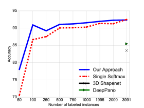
Figure 7: ModelNet10 compared to 3D Shapenet [46] and DeepPano [37] averaged over 3 trials.

The ModelNet datasets were introduced in [46] to evaluate 3D shape classifiers. ModelNet has $151,128$ 3D models classified into $40$ object categories, and ModelNet10 is a subset based on classes in the NYUv2 dataset [38]. The 3D models are voxelized to fit a $30\times 30\times 30$ grid and augmented by $12$ rotations. For the discriminative model we use a convolutional architecture similar to that of [27] where we have a 3D convolutional layer with $32$ filters of size $5$ and stride $2$, convolution of size $3$ and stride $1$, max-pooling layer with size $2$ and a $128$-dimensional fully connected layer. Similar to the CIFAR-10 experiment, we share the parameters of the last fully connected layer between the infinite mixture of VAEs and the discriminative softmax.

As shown in Figure 7, when using the whole dataset our infinite mixture and the best result from [27] match at $92\%$ accuracy. However, as we reduce the number of labeled training examples it is clear that our approach outperforms a single softmax classifier.

Additionally, Table 5 shows the accuracy comparison of the latent representation obtained from the samples from our infinite mixture and a single VAE as measured by the performance of SVM. As seen, the expected latent representation in our approach is significantly more discriminative and outperforms single VAE. This is because, we take into account the variations in the input and adapt to the complexity of the input. While a single VAE has to capture the dataset in its entirety, our approach is free to choose and fit.

Method/Labels	100	1000	All
VAE latent+SVM	64.21	79.09	82.71
Mixture latent+SVM	74.01	83.26	85.68

Table 5: ModelNet10 accuracy of latent variable representation for training SVM using a single VAE versus expected latent variable in our approach.

Our experiments with both 2D and 3D images show the initial convolutional layers play a crucial rule for the VAEs to be able to encode the input into a latent space where the mixture of experts best perform. This 3D model further illustrate the decision function mostly depends on the internal structure of the generative model rather than reconstruction of the pixel values. When we share the parameters of the discriminative model with the generative infinite mixture of VAEs and learn the mixture of experts, we combine various representations of the data for better prediction.

7 Conclusion

In this paper, we employed Bayesian non-parametric methods to propose an infinite mixture of variational autoencoders that can grow to represent the complexity of the input. Furthermore, we used these autoencoders to create a mixture of experts model for semi-supervised learning. In both 2D images and 3D shapes, our approach provides state of the art results in various datasets.

We further showed that such mixtures, where each component learns to represent a particular aspect of the data, are able to produce better predictions using fewer total parameters than a single monolithic model. This applies whether the model is generative or discriminative. Moreover, in semi-supervised learning where the ultimate objective is classification, parameter sharing between discriminative and generative models was shown to provide better prediction accuracy.

In future works we plan to extend our approach to use variational inference rather than sampling for better efficiency. In addition, a new variational loss that minimizes the joint probability of the input and output in a Bayesian paradigm may further increase the prediction accuracy when the number of labeled examples is small.

Appendix A Mathematical Details of the Infinite Variational Autoencoder

We have the following

$$p(\mathbf{c},\boldsymbol{\theta},\mathbf{x}_{1,\ldots,n},\alpha) = \int\int p_{\boldsymbol{\theta}}(\mathbf{x}_{1,\ldots,n}|\mathbf{c},\mathbf{z})p(\mathbf{z})p(\mathbf{c}|\boldsymbol{\pi})p(\boldsymbol{\pi}|\alpha)d\boldsymbol{\pi}d\mathbf{z}$$

$$= \int p_{\boldsymbol{\theta}}(\mathbf{x}_{1,\ldots,n}|\mathbf{c},\mathbf{z})p(\mathbf{z})\bigg{[}\int p(\mathbf{c}|\boldsymbol{\pi})p(\boldsymbol{\pi}|\alpha)d\boldsymbol{\pi}\bigg{]}d\mathbf{z}$$

$$= \int\left(\bigg{[}\prod_{i}^{n}p{}_{\boldsymbol{\theta}_{\mathbf{c}_{i}}}(\mathbf{x}_{i}|\mathbf{z}_{\mathbf{c}_{i}})p(\mathbf{z}_{\mathbf{c}_{i}})\bigg{]}\bigg{[}\int p(\mathbf{c}|\boldsymbol{\pi})p(\boldsymbol{\pi}|\alpha)d\boldsymbol{\pi}\bigg{]}\right)d\mathbf{z}_{\mathbf{c}_{i}}.$$

To perform inference so that the distributions of the unknown parameters are known, we use blocked Gibbs sampling by iterating the following two steps:

1. Sample for the unknown density of the observations with parameter $\boldsymbol{\theta}$ (we drop $\alpha$because it is conditionally independent $\mathbf{x}$):

   $$\mathbf{x}_{1,\ldots,n},\boldsymbol{\theta} \sim p(\mathbf{x}_{1,\ldots,n},\boldsymbol{\theta}|\mathbf{c})$$

2. Sample the base VAE assignments:

   $$\qquad\quad\mathbf{c} \sim p(\mathbf{c}|\mathbf{x}_{1,\ldots,n},\boldsymbol{\theta},\alpha)$$

For the first step, we use variational inference to find joint probability of the input and its parameter $\boldsymbol{\theta}$ conditioned on current assignments. Using standard variational inference, we have,

$$p(\mathbf{x}_{1,\ldots,n},\boldsymbol{\theta}|\mathbf{c}) = \int\prod_{i}p_{\boldsymbol{\theta}_{\mathbf{c}_{i}}}(\mathbf{x}_{i}|\mathbf{z}_{\mathbf{c}_{i}})p(\mathbf{z}_{\mathbf{c}_{i}})d\mathbf{z}_{\mathbf{c}_{i}}$$

$$= \int\prod_{i}\frac{p_{\boldsymbol{\theta}_{\mathbf{c}_{i}}}(\mathbf{x}_{i}|\mathbf{z}_{\mathbf{c}_{i}})p_{\boldsymbol{\theta}}(\mathbf{z}_{\mathbf{c}_{i}})}{q_{\phi}(\mathbf{z}_{\mathbf{c}_{i}}|\mathbf{x}_{i})}q_{\phi}(\mathbf{z}_{\mathbf{c}_{i}}|\mathbf{x}_{i})d\mathbf{z}_{\mathbf{c}_{i}}$$

$$= \int\prod_{i}p_{\boldsymbol{\theta}_{\mathbf{c}_{i}}}(\mathbf{x}_{i}|\mathbf{z}_{\mathbf{c}_{i}})\frac{p_{\boldsymbol{\theta}}(\mathbf{z}_{\mathbf{c}_{i}})}{q_{\phi}(\mathbf{z}_{\mathbf{c}_{i}}|\mathbf{x}_{i})}q_{\phi}(\mathbf{z}_{\mathbf{c}_{i}}|\mathbf{x}_{i})d\mathbf{z}_{\mathbf{c}_{i}}$$

Taking the $\log$ from both sides and using Jensen’s inequality, we have the following lower bound for the joint distribution of the observations conditioned on the latent variable assignments (VAE assignments in the infinite mixture):

$$\log\left(p(\mathbf{x}_{1,\ldots,n},\boldsymbol{\theta}|\mathbf{c})\right) \geq \sum_{i}-\text{KL}\left(q_{\phi}(\mathbf{z}_{\mathbf{c}_{i}}|\mathbf{x}_{i})\|p_{\boldsymbol{\theta}}(\mathbf{z}_{\mathbf{c}_{i}})\right)+\mathbb{E}_{q_{\phi}(\mathbf{z}|\mathbf{x}_{i})}[\log p_{\boldsymbol{\theta}_{\mathbf{c}_{i}}}(\mathbf{x}_{i}|\mathbf{z}_{\mathbf{c}_{i}})].$$ (6)

$$=\sum_{i}\mathbb{E}_{q_{\phi}(\mathbf{z}|\mathbf{x}_{i})}[\log p_{\boldsymbol{\theta}_{\mathbf{c}_{i}}}(\mathbf{x}_{i},\mathbf{z}_{\mathbf{c}_{i}})-\log q_{\phi}(\mathbf{z}_{\mathbf{c}_{i}}|\mathbf{x}_{i})]$$

Here, $\boldsymbol{\theta}$ denotes all the parameters in the decoder network and $\phi$ all the parameters in the encoder. Now, to compute the expectations in both the KL-divergence and the conditional likelihood of the second term, we use the sampling with the reparameterization trick. Thus, Equation 6 is rewritten as

$$\mathbb{E}_{q_{\phi}(\mathbf{z}|\mathbf{x}_{i})}[\log p_{\boldsymbol{\theta}_{\mathbf{c}_{i}}}(\mathbf{x}_{i},\mathbf{z}_{\mathbf{c}_{i}})-\log q_{\phi}(\mathbf{z}_{\mathbf{c}_{i}}|\mathbf{x}_{i})] \approx \frac{1}{L}\sum_{\ell=1}^{L}\log p_{\boldsymbol{\theta}_{\mathbf{c}_{i}}}(\mathbf{x}_{i},\mathbf{z}_{\mathbf{c}_{i}}^{\ell})-\log q_{\phi}(\mathbf{z}_{\mathbf{c}_{i}}^{\ell}|\mathbf{x}_{i})$$

where $\mathbf{z}$ is taken from a differentiable function that performs a random transformation of $\mathbf{x}$. This differentiable transformation function allows for using stochastic gradient descent in backpropagation algorithm. We use $L=2$ in our experiments.

For sampling the base VAE assignment $\mathbf{c}$, we know that

$$p(\mathbf{c}|\mathbf{x}_{1,\ldots,n},\boldsymbol{\theta},\alpha) = \int\underbrace{p(\mathbf{c}|\mathbf{x}_{1,\ldots,n},\boldsymbol{\theta},\boldsymbol{\pi})}_{\text{Multinomial distribution}}\underbrace{p(\boldsymbol{\pi}|\alpha)}_{\text{Dirichlet distribution}}d\boldsymbol{\pi}$$

This integral corresponds to a Multinomial distribution with Dirichlet prior where the number of components $C$ is a constant. We have,

$$p(\mathbf{c}_{1}\ldots,\mathbf{c}_{C}|\mathbf{x}_{1,\ldots,n},\boldsymbol{\theta},\boldsymbol{\pi}) = \prod_{j}^{C}\boldsymbol{\pi}_{j}^{n_{j}},\qquad\qquad n_{j}=p_{\boldsymbol{\theta}_{j}}(\mathbf{c}_{i}=j|\mathbf{x}_{i})\times\sum_{i=1}^{n}\mathbb{I}[\mathbf{c}_{i}=j],$$

Using the standard Dirichlet integration, we have

$$p(\mathbf{c}_{1}\ldots,\mathbf{c}_{C}|\mathbf{x}_{1,\ldots,n},\boldsymbol{\theta}) = \int p(\mathbf{c}_{1}\ldots,\mathbf{c}_{C}|\mathbf{x}_{1,\ldots,n},\boldsymbol{\theta},\boldsymbol{\pi}_{1},\ldots,\boldsymbol{\pi}_{C})p(\boldsymbol{\pi}_{1},\ldots,\boldsymbol{\pi}_{C})d\boldsymbol{\pi}_{1},\ldots,\boldsymbol{\pi}_{C}$$

$$= \frac{\Gamma(\alpha)}{\Gamma(\alpha+n)}\prod_{j=1}^{C}\frac{\Gamma(n_{j}+\alpha/C)}{\Gamma(\alpha/C)}$$

where we can draw samples from the conditional probabilities as

$$p(\mathbf{c}_{i}|\mathbf{c}_{i-1},\mathbf{c}_{i+1}\ldots,\mathbf{c}_{C},\mathbf{x}_{1,\ldots,n},\boldsymbol{\theta}) = \frac{\eta_{j}(\mathbf{x}_{i})+\alpha/C}{n-1+\alpha}.$$

When taking the number of components to approach infinity, $C\to\infty$ it is easy to see that the results in the paper is obtained.

Appendix B Base Variational Autoencoder’s Architecture

The base autoencoder contains the following layers:

1. Input layer: Depending on the type of the input it’s dimensions are different.

2. A fully connected layer with the number of hidden dimensions $\mathbf{h}$. This number of hidden dimensions is what is changed during training and infinite mixture uses infinite hidden dimensions. We use batch normalization in the input of this layer that according to our experiments helps with the convergence and better performance. The output of the batch normalization is used in $\tanh$ nonlinearity units. The original VAE paper did not use batch normalization.

3. The output of the last hidden layer is used in another fully connected layer with linear units to estimate the mean of the density layer $\mu$. This is the mean of the Gaussian density of the latent variable $\mathbf{z}$. Since this density is multivariate, we found $10$ percent of the hidden dimensions to performing the best. For the Dogs experiment in the paper, we used $2$-dimensional latent space.

4. Similar to the mean layer $\mu$, we have another layer with the same dimensions for estimating the diagonal entries of the density of the latent space $\sigma$.

5. For the decoder, we need to sample from the density of the latent variable $\mathbf{z}$ to compute the reconstruction. We use two samples though-out our experiments to estimate the expected reconstruction following below steps for the decoder:

   1. Sample from the latent multivariate Gaussian distribution with mean $\mu$ and variance $\sigma$.

   2. The sample is used in another fully connected layer with hidden dimensions $\mathbf{h}$. We use batch normalization in the input of this layer too. Batch normalization helps with searching for a latent space in a lower dimensions. The output of the batch normalization is used in $\tanh$ nonlinearity units.

   3. The output of the batch normalized latent space is used in another fully connected layer with sigmoid nonlinearity unit to reconstruct the input.

It should be noted that this non-symmetric autoencoder corresponds to the binary VAE described in the original paper (with minor changes that helped with its convergence stability and performance). We found this architecture to perform better than its alternative symmetric one for the semi-supervised learning application of ours for CIFAR-10 and MNIST. In evaluation of the model for computing the loss, we use the cross-entropy measure for $p(\mathbf{x}|\mathbf{z})$ since the variables are considered binary.

For 3D ModelNet and Dogs dataset, we use a symmetric variant that showed to be more effective. In the symmetric version, we changed all the $\tanh$ units to softplus ( $\log(1+\exp(x))$). The final step 5c is changed to the following: We use the hidden layer $\mathbf{h}$ to feed into two fully connected layers for the mean and variance of the decoder $\mu_{\text{dec}}$, $\sigma_{\text{dec}}$. We then sample from this decoding density for the reconstruction of the input. For computing the loss, we just use the log-likelihood of the reconstruction.

All the code is implemented in Python using Lasagne and Theano. We will release the code for the submission amongst with the dogs dataset.

References

- [1] E. Abbasnejad, S. Sanner, E. V. Bonilla, and P. Poupart. Learning community-based preferences via dirichlet process mixtures of gaussian processes. In Proceedings of the Twenty-Third International Joint Conference on Artificial Intelligence, IJCAI ’13, pages 1213–1219. AAAI Press, 2013.
- [2] P. Bachman, O. Alsharif, and D. Precup. Learning with pseudo-ensembles. In Z. Ghahramani, M. Welling, C. Cortes, N. D. Lawrence, and K. Q. Weinberger, editors, Advances in Neural Information Processing Systems 27, pages 3365–3373. Curran Associates, Inc., 2014.
- [3] K. Chen and S. Wang. Regularized boost for semi-supervised learning. In J. C. Platt, D. Koller, Y. Singer, and S. T. Roweis, editors, Advances in Neural Information Processing Systems 20, pages 281–288. Curran Associates, Inc., 2008.
- [4] M. Côté and H. Larochelle. An infinite restricted boltzmann machine. CoRR, abs/1502.02476, 2015.
- [5] D. Dai and L. V. Gool. Ensemble projection for semi-supervised image classification. In Proceedings of the 2013 IEEE International Conference on Computer Vision, ICCV ’13, pages 2072–2079, Washington, DC, USA, 2013. IEEE Computer Society.
- [6] S. Ebert, M. Fritz, and B. Schiele. Semi-Supervised Learning on a Budget: Scaling Up to Large Datasets, pages 232–245. Springer Berlin Heidelberg, Berlin, Heidelberg, 2013.
- [7] Y. Fu and L. Sigal. Semi-supervised vocabulary-informed learning. CVPR, 2016.
- [8] A. Gelman, J. B. Carlin, and H. S. Stern. Bayesian data analysis, volume 2. 2014.
- [9] I. Goodfellow, J. Pouget-Abadie, M. Mirza, B. Xu, D. Warde-Farley, S. Ozair, A. Courville, and Y. Bengio. Generative adversarial nets. In Z. Ghahramani, M. Welling, C. Cortes, N. D. Lawrence, and K. Q. Weinberger, editors, Advances in Neural Information Processing Systems 27, pages 2672–2680. Curran Associates, Inc., 2014.
- [10] I. J. Goodfellow, A. Courville, and Y. Bengio. Large-scale feature learning with spike-and-slab sparse coding. In International Conference on Machine Learning, 2012.
- [11] I. J. Goodfellow, D. Warde-Farley, M. Mirza, A. Courville, and Y. Bengio. Maxout Networks. ArXiv e-prints, Feb. 2013.
- [12] K. He, X. Zhang, S. Ren, and J. Sun. Deep residual learning for image recognition. CoRR, abs/1512.03385, 2015.
- [13] N. L. Hjort, C. Holmes, P. Müller, and S. G. Walker. Bayesian nonparametrics, volume 28. Cambridge University Press, 2010.
- [14] K. In Kim, J. Tompkin, H. Pfister, and C. Theobalt. Semi-supervised learning with explicit relationship regularization. In The IEEE Conference on Computer Vision and Pattern Recognition (CVPR), June 2015.
- [15] F. Kang, R. Jin, and R. Sukthankar. Correlated label propagation with application to multi-label learning. In Proceedings of the 2006 IEEE Computer Society Conference on Computer Vision and Pattern Recognition - Volume 2, CVPR ’06, pages 1719–1726, Washington, DC, USA, 2006. IEEE Computer Society.
- [16] D. Kingma and J. Ba. Adam: A Method for Stochastic Optimization. ArXiv e-prints, Dec. 2014.
- [17] D. P. Kingma, S. Mohamed, D. J. Rezende, and M. Welling. Semi-supervised learning with deep generative models. In Z. Ghahramani, M. Welling, C. Cortes, N. Lawrence, and K. Weinberger, editors, Advances in Neural Information Processing Systems 27, pages 3581–3589. Curran Associates, Inc., 2014.
- [18] D. P. Kingma and M. Welling. Auto-encoding variational bayes. In The International Conference on Learning Representations (ICLR), 2014.
- [19] A. Krizhevsky and G. Hinton. Learning multiple layers of features from tiny images. 2009.
- [20] A. Krizhevsky, I. Sutskever, and G. E. Hinton. Imagenet classification with deep convolutional neural networks. In P. Bartlett, F. Pereira, C. Burges, L. Bottou, and K. Weinberger, editors, Advances in Neural Information Processing Systems 25, pages 1106–1114. 2012.
- [21] H. Larochelle, M. Mandel, R. Pascanu, and Y. Bengio. Learning algorithms for the classiffcation restricted boltzmann machine. In Journal of Machine Learning Research, 2012.
- [22] A. B. L. Larsen, S. K. SÞnderby, H. Larochelle, and O. Winther. Autoencoding beyond pixels using a learned similarity metric. In The 33rd International Conference on Machine Learning, 2016.
- [23] D.-H. Lee. Pseudo-label: The simple and efficient semi-supervised learning method for deep neural networks. In Workshop on Challenges in Representation Learning, ICML, volume 3, page 2, 2013.
- [24] C. Leistner, A. Saffari, J. Santner, and H. Bischof. Semi-supervised random forests. ICCV, 2009.
- [25] A. Makhzani, J. Shlens, N. Jaitly, and I. Goodfellow. Adversarial autoencoders. arXiv preprint arXiv:1511.05644, 2015.
- [26] P. K. Mallapragada, R. Jin, A. K. Jain, and Y. Liu. Semiboost: Boosting for semi-supervised learning. IEEE Trans. Pattern Anal. Mach. Intell., 31(11):2000–2014, Nov. 2009.
- [27] D. Maturana and S. Scherer. VoxNet: A 3D Convolutional Neural Network for Real-Time Object Recognition. In IROS, 2015.
- [28] I. Misra, A. Shrivastava, and M. Hebert. Watch and learn: Semi-supervised learning of object detectors from videos. CoRR, abs/1505.05769, 2015.
- [29] T. Miyato, S.-i. Maeda, M. Koyama, K. Nakae, and S. Ishii. Distributional smoothing with virtual adversarial training. In International Conference on Learning Representation, 2016.
- [30] K. P. Murphy. Machine Learning: A Probabilistic Perspective. MIT Press, 2012.
- [31] P. Orbanz and Y. W. Teh. Bayesian nonparametric models. In Encyclopedia of Machine Learning, pages 81–89. Springer, 2011.
- [32] N. Pitelis, C. Russell, and L. Agapito. Semi-supervised Learning Using an Unsupervised Atlas, pages 565–580. Springer Berlin Heidelberg, Berlin, Heidelberg, 2014.
- [33] Y. Pu, X. Yuan, A. Stevens, C. Li, and L. Carin. A Deep Generative Deconvolutional Image Model. ArXiv e-prints, Dec. 2015.
- [34] A. Rasmus, H. Valpola, M. Honkala, M. Berglund, and T. Raiko. Semi-supervised learning with ladder networks. In Proceedings of the 28th International Conference on Neural Information Processing Systems, NIPS’15, pages 3546–3554, Cambridge, MA, USA, 2015. MIT Press.
- [35] C. E. Rasmussen. The infinite gaussian mixture model. In In Advances in Neural Information Processing Systems 12, pages 554–560. MIT Press, 2000.
- [36] C. E. Rasmussen and Z. Ghahramani. Infinite mixtures of gaussian process experts. In T. G. Dietterich, S. Becker, and Z. Ghahramani, editors, Advances in Neural Information Processing Systems 14, pages 881–888. MIT Press, 2002.
- [37] B. Shi, S. Bai, Z. Zhou, and X. Bai. Deeppano: Deep panoramic representation for 3-d shape recognition. IEEE Signal Processing Letters, 22(12):2339–2343, Dec 2015.
- [38] N. Silberman, D. Hoiem, P. Kohli, and R. Fergus. Indoor segmentation and support inference from rgbd images. In Proceedings of the 12th European Conference on Computer Vision - Volume Part V, ECCV’12, pages 746–760, Berlin, Heidelberg, 2012. Springer-Verlag.
- [39] J. T. Springenberg, A. Dosovitskiy, T. Brox, and M. Riedmiller. Striving for simplicity: The all convolutional net. arXiv preprint arXiv:1412.6806, 2014.
- [40] R. K. Srivastava, K. Greff, and J. Schmidhuber. Highway Networks. ArXiv e-prints, May 2015.
- [41] P. Vincent, H. Larochelle, I. Lajoie, Y. Bengio, and P.-A. Manzagol. Stacked denoising autoencoders: Learning useful representations in a deep network with a local denoising criterion. Journal of Machine Learning Research, 11(Dec):3371–3408, 2010.
- [42] C. Wang, S. Yan, L. Zhang, and H.-J. Zhang. Multi-label sparse coding for automatic image annotation. In Computer Vision and Pattern Recognition, 2009. CVPR 2009. IEEE Conference on, pages 1643–1650. IEEE, 2009.
- [43] Y.-X. Wang and M. Hebert. Model recommendation: Generating object detectors from few samples. In CVPR, 2015.
- [44] J. Weston, S. Chopra, and A. Bordes. Memory networks. CoRR, abs/1410.3916, 2014.
- [45] J. Weston, F. Ratle, H. Mobahi, and R. Collobert. Deep Learning via Semi-supervised Embedding, pages 639–655. Springer Berlin Heidelberg, Berlin, Heidelberg, 2012.
- [46] Z. Wu, S. Song, A. Khosla, F. Yu, L. Zhang, X. Tang, and J. Xiao. 3d shapenets: A deep representation for volumetric shapes. In The IEEE Conference on Computer Vision and Pattern Recognition (CVPR), June 2015.
- [47] Z.-H. Zhou. When semi-supervised learning meets ensemble learning. Frontiers of Electrical and Electronic Engineering in China, 6(1):6–16, 2011.