Higher-order vector discrete rogue-wave states in the coupled Ablowitz-Ladik equations: exact solutions and stability

Abstract

This paper has been accepted for publication in Chaos (2016).

An integrable system of two-component nonlinear Ablowitz-Ladik (AL) equations is used to construct complex rogue-wave (RW) solutions in an explicit form. First, the modulational instability of continuous waves is studied in the system. Then, new higher-order discrete two-component RW solutions of the system are found by means of a newly derived discrete version of a generalized Darboux transformation. Finally, perturbed evolution of these RW states is explored in terms of systematic simulations, which demonstrates that tightly and loosely bound RWs are, respectively, nearly stable and strongly unstable solutions.

Since the rogue waves (RWs) were identified from observations in the deep ocean, they have been shown to appear in many fields of nonlinear science, such as nonlinear optics, Bose-Einstein condensates, plasma physics, and even financial dynamics. The RWs can be produced as complex solutions of various nonlinear wave equations – first of all, the nonlinear Schrödinger (NLS) equation with the self-focusing cubic nonlinearity. In the framework of the integrable NLS equation, RW solutions can be generated from trivial ones by means of the Darboux transform (DT). Generally, a majority of theoretical studies of the RWs addressed models based on continuous partial differential equations, except for a few results which produced discrete RWs in integrable discrete systems, including the Ablowitz-Ladik (AL) equation (an integrable discretization of the NLS equation) and discrete Hirota equation. A natural possibility is to extend the search for RW states to coupled (first of all, two-component) systems of nonlinear wave equations. The present work aims to construct complex (higher-order) discrete RW solutions in an integrable system of two AL equations with self-attractive nonlinear terms. For this purpose, we derive a newly generalized DT method for the system, and then use it to generate higher-order discrete RW states. Then, perturbed evolution of these RWs is investigated, in a systematic form, by means of numerical simulations. It is concluded that the RW states with a tightly bound structure are quasi-stable, while their loosely bound counterparts are subject to a strong instability.

I Introduction

Cubic nonlinear Schrödinger (NLS) equations model a great variety of phenomena in many fields of nonlinear science, including nonlinear optics, water waves, plasma physics, superconductivity, Bose-Einstein condensates (BECs), and even financial dynamics soliton -f3 . A class of unstable but physically meaningful solutions of the cubic NLS equation represents rogue waves (RWs), which spontaneously emerge due to the modulational instability (MI) of continuous-wave (CW) states and then disappear RW1 ; RW2 . Recently, some new RW structures generated by the self-focusing NLS equation and some of its extensions were found, see, e.g., Refs. f3 -yuan16 . Most of these works studied continuous models, except for a few works which addressed the single-component Ablowitz-Ladik (AL) equation Ablowitz and discrete Hirota equation, using the modified bilinear method nail1d ; nail2d ; yang14 and the generalized discrete Darboux transformation wen-yan . Being a fundamentally important mathematical model, the AL equation does not find many physical realizations, but it can be implemented, in principle, as a model of arrayed optical waveguides optics , and as a mean-field limit of generalized Bose-Hubbard model for BECs trapped in a deep optical-lattice potential Kuba .

There also exist interesting coupled discrete nonlinear wave systems – in particular, coupled AL equations:

$$\begin{array}[]{ll}R_{n,t}=-i(\sigma+|R_{n}|^{2})({S_{n}}^{\ast}+{S_{n-1}}^{\ast}),\vspace{0.1in}&\\ S_{n,t}=i(\sigma+|S_{n}|^{2})({R_{n+1}}^{\ast}+{R_{n}}^{\ast}),&\end{array}$$ (1)

where $n$ denotes the discrete spatial variable, and $t$ stands for time, $R_{n}\equiv R_{n}(t)$ and $S_{n}\equiv S_{n}(t)$ are the lattice dynamical variables, $\left\{R_{n,t},S_{n,t}\right\}\equiv d\left\{R_{n},S_{n}\right\}/dt$, and the asterisk stands for the complex conjugate, while $\sigma=+1$ and $-1$ correspond, respectively, to the self-focusing and defocusing signs of the nonlinearity. System (1) is an integrable system, which represents a special two-field reduction of the four-field AL equation introduced and solved by means of the inverse-scattering transform in Ref. Ablowitz (a more general nonintegrable form of coupled AL equations was introduced in Ref. MY ). $N$-soliton solutions of Eq. (1), obtained in terms of determinants, and the derivation of infinitely many conservation laws for this system in the defocusing case, with $\sigma=-1$, by means of the $N$-fold Darboux transform (DT), were reported in Ref. wen1 . More recently, discrete vector (two-component) RW solutions of the coupled AL equations,

$$i\psi_{n,t}^{(j)}+\frac{1}{2h^{2}}(\psi_{n-1}^{(j)}+\psi_{n+1}^{(j)}-2\psi_{n}^{(j)})+\frac{1}{2}(\psi_{n-1}^{(j)}+\psi_{n+1}^{(j)})(|\psi_{n}^{(j)}|^{2}+|\psi_{n}^{(3-j)}|^{2})\quad(j=1,2),$$ (2)

were produced too, using a special transformation nail3 .

To the best of our knowledge, higher-order discrete RW solutions of system (1) have not been investigated before. A new generalized $(n,N-n)$-fold DT technique, generating higher-order RWs, was developed for some continuous nonlinear wave equations yan-wen-pre ; yan-wen-chaos , but it is still an issue how to apply a similar technique to discrete nonlinear equations. The present paper addresses this issue for discrete coupled equations (1). The key feature of such a technique is the fact that the Lax pair associated with the integrable nonlinear differential-difference equations is covariant under the gauge transformation wen1 ; wen2 .

The rest of the paper is arranged as follows. In Sec. II, we investigate the MI in the framework of Eq. (1), starting with its CW solution. In Sec. III, based on its Lax pair, a new $N$-fold DT for Eq. (1) is constructed, which can be used to derive $N$-soliton solutions from the zero seed solution, and $N$-breather solutions from the CW seed solutions of Eq. (1). Then we present a novel idea, allowing one to derive discrete versions of the generalized $(1,N-1)$-fold (using one spectral parameter) and $(M,N-M)$-fold (using $M<N$ spectral parameters) DTs for Eq. (1), by means of the Taylor expansion and a limit procedure related to the $N$-fold Darboux matrix. In Sec. IV, the generalized $(1,N-1)$-fold D is used to find discrete higher-order vector RW solutions of Eq. (1). We also analyze RW structures and their dynamical behavior by means of numerical simulations. The paper is concluded by Sec. V.

II Modulational instability of continuous waves

The simplest solution of system (1) with $\sigma=1$ (the self-focusing nonlinearity) is the CW state:

$$R_{0}(n,t)=ice^{2i(c^{2}+1)t},\quad S_{0}(n,t)=ice^{-2i(c^{2}+1)t}$$ (3)

with the real amplitude $c\not=0$. Investigation of the MI of this state is the first step towards the construction of the RW modes, as they are actually produced by the instability of the CW background RW1 ; RW2 .

We begin the analysis of the MI, taking the perturbed form of the CW as

$$R_{n}(t)=[ic+\varepsilon r_{n}(t)]e^{2i(c^{2}+1)t},\ \ \ S_{n}(t)=[ic+\varepsilon s_{n}^{\ast}(t)]e^{-2i(c^{2}+1)t},$$ (4)

where $\varepsilon$ is an infinitesimal amplitude of the perturbation. The substitution of wave form (4) into system (1) yields a linearized system,

$$\begin{array}[]{ll}r_{n,t}+2i\left(r_{n}+c^{2}r_{n}^{*}\right)+i\left(c^{2}+1\right)\left(s_{n}+s_{n-1}\right)=0,\vspace{0.1in}&\\ s_{n,t}+2i\left(s_{n}+c^{2}s_{n}^{*}\right)+i\left(c^{2}+1\right)\left(r_{n+1}+r_{n}\right)=0.&\end{array}$$ (5)

To analyze the MI on the basis of the complex linearized equation (5), each component of the perturbation may be split into real and imaginary parts: $r_{n}(t)\equiv r_{1n}(t)+ir_{2n}(t),~{}s_{n}(t)\equiv s_{1n}(t)+is_{2n}(t)$, which transform the system of two complex equations (5) into a system of four real equations:

$$\begin{array}[]{l}r_{1n,t}+2\left(c^{2}-1\right)r_{2n}-(c^{2}+1)\left(s_{2n}+s_{2,n-1}\right)=0,\vspace{0.1in}\\ r_{2n,t}+2\left(c^{2}+1\right)r_{1n}+(c^{2}+1)\left(s_{1n}+s_{1,n-1}\right)=0,\vspace{0.1in}\\ s_{1n,t}+2\left(c^{2}-1\right)s_{2n}-(c^{2}+1)\left(r_{2,n+1}+r_{2n}\right)=0,\vspace{0.1in}\\ s_{2n,t}+2\left(c^{2}+1\right)s_{1n}+(c^{2}+1)\left(r_{1,n+1}+r_{1n}\right)=0.\end{array}$$ (6)

Solutions to these real equations may be sought for in a formally complex form,

$$\left\{r_{1n}(t),\,r_{2n}(t),\,s_{1n}(t),\,s_{2n}(t)\right\}=\left\{r_{1n}^{(0)},\,r_{2n}^{(0)},\,s_{1n}^{(0)},\,s_{2n}^{(0)}\right\}e^{gt+ikn},$$ (7)

where $g$ is the MI gain (generally, this eigenvalue may be complex), and $k$ an arbitrary real wavenumber of the small perturbation, while $r_{1n}^{(0)},\,r_{2n}^{(0)},\,s_{1n}^{(0)},\,s_{2n}^{(0)}$ are constant amplitudes of the perturbation eigenmode. The substitution of this ansatz in Eq. (7) into system (6) produces an MI dispersion equation in the form of the determinant,

$$\left|\begin{array}[]{cccc}g&2(c^{2}-1)&0&-(c^{2}+1)(1+e^{-ik})\vspace{0.1in}\\ 2(c^{2}+1)&g&(c^{2}+1)(1+e^{-ik})&0\vspace{0.1in}\\ 0&-(c^{2}+1)(1+e^{ik})&g&2(c^{2}-1)\vspace{0.1in}\\ (c^{2}+1)(1+e^{ik})&0&2(c^{2}+1)&g\end{array}\right|=0,$$ (8)

which leads to an explicit dispersion relation:

$$g^{2}=2(c^{2}+1)\left[c^{2}-(c^{2}+1)\cos k-3\pm 2\sqrt{2(1+\cos k)}\right].$$ (9)

Therefore, the MI occurs when expression (9) is positive, the branch with sign $+$ being always dominant. In particular, it is easy to check that the MI condition $g^{2}>0$ holds for all $k$, provided that the CW amplitude is large enough, viz., $c^{2}>1$. To illustrate this property, Fig. 1 displays the positive root $g(k)$ for $c=2,3,$ and $5$. Furthermore, at point

$$\cos k=2\left(c^{2}+1\right)^{-2}-1$$ (10)

(note that it obeys constraint $\left|\cos k\right|<1$), Eq. (9) yields $g_{\max}^{2}=4c^{4}$, hence the MI takes place at all finite values of amplitude $c$. In fact, $g_{\max}^{2}$ is the largest value attained by $g^{2}\left(\cos k\right)$ at any $c$, i.e., Eq. (10) determines wavenumbers of the dominant MI perturbation eigenmodes, $k=\pm\arccos\left[2\left(c^{2}+1\right)^{-2}-1\right]+2m\pi$ with integer $m$.

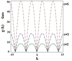
Figure 1: (color online). Gain spectra of the modulation instability for different CW amplitudes are displayed by means of positive growth rate $g(k)$, as given by Eq. (9) with sign $+$. Different lines correspond to values of the CW amplitude $c=2$ (solid), $c=3$ (dashed), and $c=5$ (dotted-dashed), as indicated in the figure.

III Generalized Darboux transform

III.1 The Lax pair and $N$-fold Darboux transform

The Lax pair of system (1) is written in the known form wen1 :

$$E\varphi_{n}=U_{n}\varphi_{n},\qquad U_{n}=\left(\begin{array}[]{cc}\lambda+R_{n}S_{n}&-\sigma{R_{n}}^{\ast}+\lambda^{-1}S_{n}\vspace{0.1in}\\ R_{n}-\sigma\lambda{S_{n}}^{\ast}&\lambda^{-1}+(R_{n}S_{n})^{\ast}\end{array}\right),$$ (11)

$$\varphi_{n,t}=V_{n}\varphi_{n},\qquad V_{n}=i\left(\begin{array}[]{cc}-\lambda+(R_{n}S_{n-1})^{\ast}&\quad\sigma{R_{n}}^{\ast}+\lambda^{-1}S_{n-1}\vspace{0.1in}\\ R_{n}+\sigma\lambda{S_{n-1}}^{\ast}&\lambda^{-1}-R_{n}S_{n-1}\end{array}\right),\ \$$ (12)

where $\lambda$ is a constant iso-spectral parameter, $E$ is the shift operator defined by $Ef_{n}=f_{n+1},\ E^{-1}f_{n}=f_{n-1}$, and $\varphi_{n}=\varphi_{n}(t)=(\phi_{n}(t),\psi_{n}(t))^{T}$ (with $T$ denoting the transpose of the vector or matrix) is an eigenfunction vector. It is easy to verify that the compatibility condition, $U_{n,t}+U_{n}V_{n}-V_{n+1}U_{n}=0$, of Eqs. (11) and (12) is precisely tantamount to system (1).

In what follows, we construct a new $N$-fold DT for system (1), which is different from one reported in Ref. wen1 . For this purpose, we introduce the following gauge transformation:

$$\widetilde{\varphi}_{n}=T_{n}\varphi_{n}\ ,$$ (13)

where $T_{n}$ is an $2\times 2$ Darboux matrix to be determined, $\widetilde{\varphi}_{n}$ is required to satisfy Eqs. (11) and (12) with $U_{n}$ and $V_{n}$ replaced, respectively, by $\widetilde{U_{n}}$ and $\widetilde{V_{n}}$, i.e.,

$$E\widetilde{\varphi}_{n}=\widetilde{U}_{n}\widetilde{\varphi}_{n},\quad\widetilde{\varphi}_{n,t}=\widetilde{V}_{n}\widetilde{\varphi}_{n},$$ (14)

with $\widetilde{U}_{n}=U_{n}|_{R_{n}\rightarrow\widetilde{R}_{n},\,S_{n}\rightarrow\widetilde{S}_{n}}$ and $\widetilde{V}_{n}=V_{n}|_{R_{n}\rightarrow\widetilde{R}_{n},\,S_{n}\rightarrow\widetilde{S}_{n}}$. It follows from Eq. (13) and (14) that one has constraints

$$\widetilde{U}_{n}=T_{n+1}U_{n}{T_{n}}^{-1},\qquad\widetilde{V}_{n}=(T_{n,t}+T_{n}V_{n}){T_{n}}^{-1},$$ (15)

which lead to the DT of system (1).

The Darboux matrix $T_{n}$, which determines the gauge transformation (13) is a key element in constructing the DT of Eq. (1). We consider the matrix in the form of

$$T_{n}(\lambda)=\left(\begin{array}[]{cc}\lambda^{N}+\sum\limits_{j=0}^{N-1}a_{n}^{(j)}\lambda^{j}&\sum\limits_{j=0}^{N-1}b_{n}^{(j)}\lambda^{j}\vspace{0.1in}\\ -\sigma\sum\limits_{j=0}^{N-1}{b_{n}^{(j)}}^{\ast}\lambda^{N-j}&\quad 1+\sum\limits_{j=0}^{N-1}{a_{n}^{(j)}}^{\ast}\lambda^{N-j}\end{array}\right),$$ (16)

where $N$ is a non-negative integer, and $a_{n}^{(j)},b_{n}^{(j)}\,(j=0,1,2,...,N-1)$ are functions of $n$ and $t$ determined by the following linear algebraic system:

$$T_{n}(\lambda)\varphi(\lambda)|_{\lambda=\lambda_{k}}=0\quad(k=1,2,...,N)$$ (17)

where $\varphi(\lambda)=(\phi(\lambda),\psi(\lambda))^{T}$ is a basic solution of Eqs. (11) and (12). $N$ parameters $\lambda_{k}\ (\lambda_{k}\neq\lambda_{j}$ for $k\neq j)$ must be chosen so that the determinant of the coefficients for system (17) is different from zero, hence, $a_{n}^{(j)}$ and $b_{n}^{(j)}$ are uniquely determined by Eq. (17). It follows from Eqs. (15) and (17) that we have the following theorem:

Theorem 1.   Let $\varphi_{j}(\lambda_{j})=(\phi_{j},\psi_{j})^{T}$ be $N$ distinct column-vector solutions of the problem for spectral parameters $\lambda_{j}\,(j=1,2,..,N)$, based on Eqs. (11) and (12), and $R_{0}(n,t),\,S_{0}(n,t)$ is a seed solution of system (1); then, the new $N$-fold DT for system (1) is given by

$$\hskip 56.9055pt\widetilde{R}_{N}(n,t)=\dfrac{R_{0}(n,t)+\sigma{b_{n}^{(N-1)}}^{\ast}}{a_{n}^{(0)}},\ \ \ \widetilde{S}_{N}(n,t)=\sigma{b_{n+1}^{(0)}+S_{0}(n,t)a_{n+1}^{(0)}},$$ (18)

with $a_{n}^{(0)}=\dfrac{\Delta a_{n}^{(0)}}{\Delta_{N}},b_{n}^{(0)}=\dfrac{\Delta b_{n}^{(0)}}{\Delta_{N}},b_{n}^{(N-1)}=\dfrac{\Delta b_{n}^{(N-1)}}{\Delta_{N}},$

$$\Delta_{N}=\left|\begin{array}[]{cccccccc}\lambda_{1}^{N-1}\phi_{1}&\lambda_{1}^{N-2}\phi_{1}&\ldots&\phi_{1}&{\lambda_{1}}^{N-1}\psi_{1}&\lambda_{1}^{N-2}\psi_{1}&\ldots&\psi_{1}\vspace{0.1in}\\ \lambda_{2}^{N-1}\phi_{2}&\lambda_{2}^{N-2}\phi_{2}&\ldots&\phi_{2}&\lambda_{2}^{N-1}\psi_{2}&\lambda_{2}^{N-2}\psi_{2}&\ldots&\psi_{2}\vspace{0.1in}\\ \ldots&\ldots&\ldots&\ldots&\ldots&\ldots&\ldots&\ldots\vspace{0.1in}\\ \lambda_{N}^{N-1}\phi_{N}&\lambda_{N}^{N-2}\phi_{N}&\ldots&\phi_{N}&\lambda_{N}^{N-1}\psi_{N}&\lambda_{N}^{N-2}\psi_{N}&\ldots&\psi_{N}\vspace{0.1in}\\ \lambda_{1}^{*}\psi_{1}^{*}&\lambda_{1}^{\ast 2}\psi_{1}^{*}&\ldots&\lambda_{1}^{\ast N}\psi_{1}^{*}&-\sigma\lambda_{1}^{*}\phi_{1}^{*}&-\sigma\lambda_{1}^{\ast 2}\phi_{1}^{*}&\ldots&-\sigma\lambda_{1}^{\ast N}\phi_{1}^{*}\vspace{0.1in}\\ \lambda_{2}^{*}\psi_{2}^{*}&\lambda_{2}^{\ast 2}\psi_{2}^{*}&\ldots&\lambda_{2}^{\ast N}\psi_{2}^{*}&-\sigma\lambda_{2}^{*}\phi_{2}^{*}&-\sigma\lambda_{2}^{\ast 2}\phi_{2}^{*}&\ldots&-\sigma\lambda_{2}^{\ast N}\phi_{2}^{*}\vspace{0.1in}\\ \ldots&\ldots&\ldots&\ldots&\ldots&\ldots&\ldots&\ldots\vspace{0.1in}\\ \lambda_{N}^{*}\psi_{N}^{*}&\lambda_{N}^{\ast 2}\psi_{N}^{*}&\ldots&\lambda_{N}^{\ast N}\psi_{N}^{*}&-\sigma\lambda_{N}^{*}\phi_{N}^{*}&-\sigma\lambda_{N}^{\ast 2}\phi_{N}^{*}&\ldots&-\sigma\lambda_{N}^{\ast N}\phi_{N}^{*}\end{array}\right|,$$

where $\Delta a_{n}^{(0)}$, $\Delta b_{n}^{(0)}$ and $\Delta b_{n}^{(N-1)}$ are given by determinant $\Delta_{N}$, replacing its $N$-th, $(2N)$-th and $(N+1)$-th columns by the column vector $(-\lambda_{1}^{N}\phi_{1}$, $-\lambda_{2}^{N}\phi_{2}$,$\cdots$, $-\lambda_{N}^{N}\phi_{N}$, $-\psi_{1}^{{*}}$, $-\psi_{2}^{{*}}$,$\cdots$, $-\psi_{N}^{{*}})^{\mathrm{T}}$, while $\Delta a_{n+1}^{(0)}$ and $\Delta b_{n+1}^{(0)}$ are obtained from $\Delta a_{n}^{(0)}$ and $\Delta b_{n}^{(0)}$, replacing $n$ by $n+1$.

The proof of this theorem can be performed following the lines of Refs. wen1 ; wen2 , and this $N$-fold DT includes the known DT wen1 . The $N$-fold DT with the zero seed solutions, $R_{0}=S_{0}=0$ (or the CW, alias plane wave, solutions), can be used to construct multi-soliton solutions (or multi-breather solutions) of Eq. (1). This is not the main objective of the present work. Actually, our aim is to extend the $N$-fold DT into a generalized $(M,N-M)$-fold DT such that multi-RW solutions can be found in terms of the determinants defined above for solutions of Eq. (1).

III.2 Generalized $(1,N-1)$-fold Darboux transforms

Here we consider the Darboux matrix (16) with a single spectral parameter, $\lambda=\lambda_{1}$, rather than $N>1$ distinct parameters $\lambda_{k}\,$. Then, the respective equation (17),

$$T_{n}(\lambda_{1})\varphi(\lambda_{1})=0,$$ (19)

gives rise to two algebraic equations for $2N$ functions $a_{n}^{(j)}$ and $b_{n}^{(j)}\,(j=0,1,...,N-1)$. To determine them, we need to find additional $2(N-1)$ equations for $a_{n}^{(j)}$ and $b_{n}^{(j)}$. To generate such extra equations from Eq. (19), we consider the Taylor expansion of $T_{n}(\lambda_{1})\varphi(\lambda_{1})\big{|}_{\{\lambda_{1}\rightarrow\lambda_{1}+\varepsilon\}}=T_{n}(\lambda_{1}+\varepsilon)\varphi(\lambda_{1}+\varepsilon)$ around $\varepsilon=0$ in the form of

$$T_{n}(\lambda_{1}+\varepsilon)\varphi(\lambda_{1}+\varepsilon)=\sum_{k=0}^{N-1}\sum\limits_{j=0}^{k}T^{(j)}(\lambda_{1})\varphi^{(k-j)}(\lambda_{1})\varepsilon^{k}+\mathcal{O}(\varepsilon^{N-1}),\quad$$ (20)

and demand that all coefficients in front of $\varepsilon^{s}\,(s=0,1,2,...,N-1)$ are equal to zero, which yields

$$\begin{array}[]{r}T_{n}^{(0)}(\lambda_{1})\varphi^{(0)}(\lambda_{1})=0,\vspace{0.1in}\\ T_{n}^{(0)}(\lambda_{1})\varphi^{(1)}(\lambda_{1})+T_{n}^{(1)}(\lambda_{1})\varphi^{(0)}(\lambda_{1})=0,\vspace{0.1in}\\ T_{n}^{(0)}(\lambda_{1})\varphi^{(2)}(\lambda_{1})+T_{n}^{(1)}(\lambda_{1})\varphi^{(1)}(\lambda_{1})+T_{n}^{(2)}(\lambda_{1})\varphi^{(0)}(\lambda_{1})=0,\vspace{0.1in}\\ \qquad\cdots\cdots,\vspace{0.1in}\\ \sum\limits_{j=0}^{N-1}T_{n}^{(j)}(\lambda_{1})\varphi^{(N-1-j)}(\lambda_{1})=0.\end{array}$$ (21)

where

$$T_{n}^{(k)}(\lambda_{1})=\frac{1}{k!}\frac{\partial^{k}}{\partial\lambda_{1}^{k}}T(\lambda_{1}),\quad\varphi^{(k)}(\lambda_{1})=\frac{1}{k!}\frac{\partial^{k}}{\partial\lambda_{1}^{k}}\varphi(\lambda_{1})=\left(\frac{1}{k!}\frac{\partial^{k}}{\partial\lambda_{1}^{k}}\phi(\lambda_{1}),\,\frac{1}{k!}\frac{\partial^{k}}{\partial\lambda_{1}^{k}}\psi(\lambda_{1})\right)^{\mathrm{T}}\quad(k=0,1,2,...).$$ (22)

The first sub-system in system (21) is just Eq. (19), as required. Therefore, system (21) contains $2N$ algebraic equations for $2N$ unknowns $a_{n}^{(j)}$ and $b_{n}^{(j)}\,(j=0,1,...,N-1)$. When eigenvalue $\lambda_{1}$ is suitably chosen, so that the determinant of coefficients of system (21) does not vanish, the Darboux matrix $T_{n}$ given by Eq. (16) is uniquely determined by the new system (21) (cf. the previous condition given by Eq. (17)).

The proof of Theorem 1 only uses Eqs. (13), (15), and (16), but not Eq. (17) wen2 , therefore, if we replace system (17) by (21), which are used to determine $a_{n}^{(j)}$ and $b_{n}^{(j)}$ in Darboux matrix $T_{n}$, then Theorem 1 also holds for Darboux matrix (16) with $a_{n}^{(j)}$ and $b_{n}^{(j)}$ determined by system (21), cf. Ref. wen2 . Thus, when $a_{n}^{(j)}$ and $b_{n}^{(j)}$ in the Darboux matrix $T_{n}$ are chosen as the new functions, we can derive new solutions by using DT (18) with the single eigenvalue $\lambda=\lambda_{1}$. We call Eqs. (18) and (13), associated with new functions $a_{n}^{(j)}$ and $b_{n}^{(j)}$ determined by system (21), as a generalized $(1,N-1)$-fold DT, which leads to the following theorem for system (1).

Theorem 2. Let $\varphi(\lambda_{1})=(\phi(\lambda_{1}),\psi(\lambda_{1}))^{\mathrm{T}}$ be a column vector-solution of the problem for spectral parameter $\lambda_{1}$, based on Eqs. (11) and (12), and $R_{0}(n,t),S_{0}(n,t)$ is a seed solution of system (1); then, the generalized $(1,N-1)$-fold DT for Eq. (1) is given by

$$\hskip 56.9055pt\widetilde{R}_{N}(n,t)=\dfrac{R_{0}(n,t)+\sigma{b_{n}^{(N-1)}}^{\ast}}{a_{n}^{(0)}},\ \ \ \widetilde{S}_{N}(n,t)=\sigma{b_{n+1}^{(0)}+S_{0}(n,t)a_{n+1}^{(0)}},$$ (23)

with $a_{n}^{(0)}=\dfrac{\Delta a_{n}^{(0)}}{\Delta_{N}^{\epsilon}},\,b_{n}^{(0)}=\dfrac{\Delta b_{n}^{(0)}}{\Delta_{N}^{\epsilon}},\,b_{n}^{(N-1)}=\dfrac{\Delta b_{n}^{(N-1)}}{\Delta_{N}^{\epsilon}}$, $\Delta_{N}^{\epsilon}=\left|(\Delta_{j,s})_{2N\times 2N}\right|,$

$$\Delta_{j,s}=\begin{cases}\sum\limits_{k=0}^{j-1}C_{N-s}^{k}{\lambda_{1}}^{(N-s-k)}{\phi^{(j-1-k)}}\quad\mathrm{for}\quad 1\leq j,\,s\leq N,\vspace{0.1in}\\ \sum\limits_{k=0}^{j-1}C_{2N-s}^{k}{\lambda_{1}}^{(2N-s-k)}{\psi^{(j-1-k)}}\quad\mathrm{for}\quad 1\leq j\leq N,\,N+1\leq s\leq 2N,\vspace{0.1in}\\ \sum\limits_{k=0}^{j-(N+1)}C_{s}^{k}{\lambda_{1}}^{\ast(s-k)}{\psi^{*(j-N-1-k)}}\quad\mathrm{for}\quad N+1\leq j\leq 2N,\,1\leq s\leq N,\vspace{0.1in}\\ -\sigma\sum\limits_{k=0}^{j-(N+1)}C_{s-N}^{k}{\lambda_{1}}^{\ast(s-N-k)}{\phi^{*(j-N-1-k)}}\quad\mathrm{for}\quad N+1\leq j,\,s\leq 2N,\end{cases}$$

with $\Delta a_{n}^{(0)}$, $\Delta b_{n}^{(0)}$ and $\Delta b_{n}^{(N-1)}$ given by determinant $\Delta_{N}^{\epsilon}$, replacing its $N$-th, $(2N)$-th and $(N+1)$-th columns by the column vector $b=(b_{j})_{2N\times 1}$ with

$$b_{j}=\begin{cases}-\sum\limits_{k=0}^{j-1}C_{N}^{k}{\lambda_{1}}^{(N-k)}{\phi^{(j-1-k)}}\quad\mathrm{for}\quad 1\leq j\leq N\vspace{0.1in}\\ -{\psi^{*(j-N-1)}}\quad\mathrm{for}\quad N+1\leq j\leq 2N\end{cases}$$

Here, $\Delta a_{n+1}^{(0)}$ and $\Delta b_{n+1}^{(0)}$ are obtained from $\Delta a_{n}^{(0)}$ and $\Delta b_{n}^{(0)}$, replacing $n$ with $n+1$.

Notice that, in the symbol of the generalized $(1,N-1)$-fold DT, integer $1$ refers to the number of the spectral parameters, and $N-1$ indicates the order of the highest derivative of the Darboux matrix $T$ in system (21) (or the order of the highest derivative of the vector eigenfunction $\varphi$ in system (21)).

III.3 Generalized $(M,N-M)$-fold Darboux transforms

The generalized $(1,N-1)$-fold DT, which we have constructed using the single spectral parameter, $\lambda=\lambda_{1}$, and the highest-order derivatives of $T_{n}(\lambda_{1})$ or $\varphi(\lambda_{1})$ with $m_{1}=N-1$, can be extended to include $M<N$ spectral parameters $\lambda_{i}\,(i=1,2,...,M)$ and the corresponding highest-order derivative orders, $m_{i}\,\ (m_{i}=0,1,2,...)$, where non-negative integers $M,\,m_{i}$ are required to satisfy constraint $N=M+\sum_{i=1}^{M}m_{i}$, where $N$ is the same as in Darboux matrix $T_{n}$ (16). In the following, we consider the Darboux matrix (16) and eigenfunctions $\varphi_{i}(\lambda_{i})\,(i=1,2,...,M)$, which are solutions of the linear spectral problem for parameters $\lambda_{i}$, based on Eqs. (11) and (12), along with the seed solution $R_{0},S_{0}$ of Eq. (1). Thus we have

$$T_{n}(\lambda_{i}+\varepsilon)\varphi_{i}(\lambda_{i}+\varepsilon)\!\!=\!\!\sum_{k=0}^{+\infty}\sum\limits_{j=0}^{k}T_{n}^{(j)}(\lambda_{i})\varphi_{i}^{(k-j)}(\lambda_{i})\varepsilon^{k},$$ (24)

where $\varphi_{i}^{(k)}(\lambda_{i})$ and $T_{n}^{(k)}(\lambda_{i})$ are defined by Eq. (22) with $\lambda_{1}\to\lambda_{i}\,(k=0,1,2,...)$, and $\varepsilon$ is a small parameter.

It follows from Eq. (24) and

$$\lim\limits_{\varepsilon\rightarrow 0}\dfrac{T_{n}(\lambda_{i}+\varepsilon)\varphi_{i}(\lambda_{i}+\varepsilon)}{\varepsilon^{k_{i}}}=0,$$ (25)

with $i=1,2,...,M$ and $k_{i}=0,1,...,m_{i}$, that we obtain a linear algebraic system with the $2N$ equations ($N=M+\sum_{i=1}^{M}m_{i}$):

$$\begin{array}[]{r}T_{n}^{(0)}(\lambda_{i})\varphi_{i}^{(0)}(\lambda_{i})=0,\vspace{0.1in}\\ T_{n}^{(0)}(\lambda_{i})\varphi_{i}^{(1)}(\lambda_{i})+T_{n}^{(1)}(\lambda_{i})\varphi_{i}^{(0)}(\lambda_{i})=0,\vspace{0.1in}\\ T_{n}^{(0)}(\lambda_{i})\varphi_{i}^{(2)}(\lambda_{i})+T_{n}^{(1)}(\lambda_{1})\varphi_{i}^{(1)}(\lambda_{i})+T_{n}^{(2)}(\lambda_{i})\varphi_{i}^{(0)}(\lambda_{i})=0,\vspace{0.1in}\\ \qquad\cdots\cdots,\vspace{0.1in}\\ \sum\limits_{j=0}^{m_{i}}T_{n}^{(j)}(\lambda_{i})\varphi_{i}^{(m_{i}-j)}(\lambda_{i})=0,\end{array}$$ (26)

in which some equations for index $i$, i.e., $T_{n}^{(0)}(\lambda_{i})\varphi_{i}^{(0)}(\lambda_{i})=T_{n}(\lambda_{i})\varphi_{i}(\lambda_{i})=0$, are similar to the first equations in Eqs. (21), but they are different if there exists at least one $m_{i}\not=0$. When eigenvalues $\lambda_{i}$ $(i=1,2,..,M)$ are suitably chosen, so that the determinant of the coefficients for system (21) does not vanish, the transformation matrix $T$ is uniquely determined by system (21), and Theorem 1 still holds. Using new functions $a_{n}^{(j)}$ and $b_{n}^{(j)}$ obtained with the $N$-order Darboux matrix $T_{n}$, we can derive the new DT with $M$ distinct eigenvalues. Here, we identify Eqs. (18) and (13) as a generalized $(M,N-M)$-fold DTs for Eq. (1), which is specified by the following theorem.

Theorem 3. Let $\varphi_{i}(\lambda_{i})=(\phi_{i}(\lambda_{i}),\,\psi_{i}(\lambda_{i}))^{\mathrm{T}}$ be column-vector solutions with distinct spectral parameters $\lambda_{i}\,(i=1,2,...,M)$ of the problem based on Eqs. (11) and (12), and $(R_{0}(n,t),\,S_{0}(n,t))$ is the same seed solution of Eq. (1), as considered above, then the generalized $(M,N-M)$-fold DT for Eq. (1) is given by

$$\widetilde{R}_{N}(n,t)=\dfrac{R_{0}(n,t)+\sigma{b_{n}^{(N-1)}}^{\ast}}{a_{n}^{(0)}},\ \ \ \widetilde{S}_{N}(n,t)=\sigma{b_{n+1}^{(0)}+S_{0}(n,t)a_{n+1}^{(0)}}~{},$$ (27)

with $a_{n}^{(0)}=\dfrac{\Delta a_{n}^{(0)}}{\Delta_{N}^{\epsilon(M)}},b_{n}^{(0)}=\dfrac{\Delta b_{n}^{(0)}}{\Delta_{N}^{\epsilon(M)}},b_{n}^{(N-1)}=\dfrac{\Delta b_{n}^{(N-1)}}{\Delta_{N}^{\epsilon(M)}},\ \Delta_{N}^{\epsilon(M)}=\mathrm{det}([\Delta^{(1)}...\Delta^{(M)}]^{\mathrm{T}})$,
where $\Delta^{(i)}=(\Delta_{j,s}^{(i)})_{2(m_{i}+1)\times 2N},$  in which $\Delta_{j,s}^{(i)}\,\,(1\leq j\leq 2(m_{i}+1)$,  $1\leq s\leq N$, $i=1,2,...,M$) are given by the following expressions:

$$\Delta_{j,s}^{(i)}=\begin{cases}\sum\limits_{k=0}^{j-1}C_{N-s}^{k}{\lambda_{i}}^{(N-s-k)}{\phi^{(j-1-k)}}\quad\mathrm{for}\quad 1\leq j\leq m_{i}+1,\,1\leq s\leq N,\vspace{0.1in}\\ \sum\limits_{k=0}^{j-1}C_{2N-s}^{k}{\lambda_{i}}^{(2N-s-k)}{\psi^{(j-1-k)}}\quad\mathrm{for}\quad 1\leq j\leq m_{i}+1,\,N+1\leq s\leq 2N,\vspace{0.1in}\\ \sum\limits_{k=0}^{j-(N+1)}C_{s}^{k}{\lambda_{i}}^{\ast(s-k)}{\psi^{*(j-N-1-k)}}\quad\mathrm{for}\quad m_{i}+2\leq j\leq 2(m_{i}+1),\,1\leq s\leq N,\vspace{0.1in}\\ -\sigma\sum\limits_{k=0}^{j-(N+1)}C_{s-N}^{k}{\lambda_{i}}^{\ast(s-N-k)}{\phi^{*(j-N-1-k)}}\quad\mathrm{for}\quad m_{i}+2\leq j\leq 2(m_{i}+1),\,N+1\leq s\leq 2N,\end{cases}$$

with $\Delta a_{n}^{(0)}$, $\Delta b_{n}^{(0)}$ and $\Delta b_{n}^{(N-1)}$ given by determinant $\Delta_{N}^{\epsilon(M)}$, replacing its $N$-th, $(2N)$-th and $(N+1)$-th columns by the column vector $b=(b_{j})_{2N\times 1}$, with

$$b_{j}=\begin{cases}-\sum\limits_{k=0}^{j-1}C_{N}^{k}{\lambda_{i}}^{(N-k)}{\phi^{(j-1-k)}}\quad 1\leq j\leq m_{i}+1,\vspace{0.1in}\\ -{\psi^{*(j-N-1)}}\quad\mathrm{for}\quad m_{i}+2\leq j\leq 2(m_{i}+1).\end{cases}$$

Notice that when $M=1$ and $m_{1}=N-1$, Theorem 3 reduces to Theorem 2, and when $M=N$ and $m_{i}=0,\,1\leq i\leq N$, Theorem 3 reduces to Theorem 1. When $M\neq 1$ and $M\neq$ $N$, the procedure makes it possible to derive new DTs, which we do not explicitly discuss here. Below, we use the generalized $(1,N-1)$-fold Darboux transformation to construct multi-RW solutions of Eq. (1) from the seed CW states.

IV Higher-order vector rogue-wave solutions and dynamical behavior

In what follows we produce multi-RW solutions in terms of the determinants introduced above for Eq. (1) with $\sigma=1$ (the self-focusing nonlinearity) by means of the generalized $(1,N-1)$-fold DT. Equation (1) is similar to the NLS equation, which gives rise to RWs in the case of $\sigma=1$ (and it does not generate such solutions in the case of the self-defocusing, with $\sigma=-1$). We here take, as the seed, CW solution (3) of Eq. (1) with $\sigma=1$. The substitution of this into the Lax-pair equations (11) and (12) yields the following solution:

$$\varphi(\lambda)=C_{1}\tau^{n}e^{\rho t+\Theta(\varepsilon)}\left[\begin{array}[]{c}i\dfrac{1-\lambda-\sqrt{(\lambda-1)^{2}-4\lambda c^{2}}}{2\lambda c}\vspace{0.1in}\\ e^{2i(1+c^{2})t}\end{array}\right],$$ (28)

with

$$\begin{array}[]{l}\tau=\dfrac{\lambda^{2}-2c^{2}\lambda+1+(\lambda+1)\sqrt{(\lambda-1)^{2}-4\lambda c^{2}}}{2\lambda},\vspace{0.1in}\\ \rho=-\dfrac{\lambda^{2}+2\lambda(c^{2}+1)-1+(\lambda-1)\sqrt{(\lambda-1)^{2}-4\lambda c^{2}}}{2\lambda},\vspace{0.1in}\\ \Theta(\varepsilon)=\sqrt{(\lambda-1)^{2}-4\lambda c^{2}}\sum\limits_{k=1}^{N}(e_{k}+id_{k})\varepsilon^{2k},\end{array}$$

where $C_{1}$ is an arbitrary constant, $e_{k},d_{k}$ $(k=1,2,...,N)$ are free real coefficients, and $\varepsilon$ is an artificially introduced small parameter.

Next, we fix the spectral parameter in Eq. (28) as $\lambda=\lambda_{1}+\varepsilon^{2}$ with $\lambda_{1}=2c^{2}+1+2\sqrt{c^{2}(c^{2}+1)}$, and expand vector function $\varphi$ in Eq. (28) into the Taylor series around $\varepsilon=0$, explicitly calculating the two first coefficients of the expansion. In particular, choosing $C_{1}=1,c=\frac{3}{4}$, which yields $\lambda_{1}=4$, we obtain

$$\varphi(\varepsilon^{2})=\sum_{j=0}^{\infty}\varphi^{(j)}\varepsilon^{2j}=\varphi^{(0)}+\varphi^{(1)}\varepsilon^{2}+\varphi^{(2)}\varepsilon^{4}+\varphi^{(3)}\varepsilon^{6}+\cdots,$$ (29)

where

$$\varphi^{(0)}=\left(\begin{array}[]{c}\phi^{(0)}\\ \psi^{(0)}\end{array}\right)=\frac{1}{2}\left(\frac{25}{16}\right)^{n}\left(\begin{array}[]{c}ie^{-\frac{55}{16}it}\vspace{0.1in}\\ 2e^{-\frac{5}{16}it}\end{array}\right),\qquad\qquad\qquad\hskip 21.68121pt$$

$$\varphi^{(1)}=\frac{1}{15360}\left(\frac{25}{16}\right)^{n}\left[\begin{array}[]{c}e^{-\frac{55}{16}it}(7680t-2025it^{2}+2304in^{2}+4320nt+640i+3840in)\vspace{0.1in}\\ -6e^{-\frac{5}{16}it}(1360it+675t^{2}-768n^{2}+1440int)\end{array}\right],$$

$\varphi^{(2,3)}=(\phi^{(2,3)},\psi^{(2,3)})^{\mathrm{T}}\,$are listed in Appendix A, and $n$ denotes the discrete spatial variable.

It follows from Eqs. (13), (18), and (29) that we can derive new exact RW solutions of Eq. (1) as follows:

$$\hskip 28.45274pt\widetilde{R}_{N}(n,t)=\dfrac{R_{0}(n,t)+{b_{n}^{(N-1)}}^{\ast}}{a_{n}^{(0)}},\ \ \ \widetilde{S}_{N}(n,t)={b_{n+1}^{(0)}+S_{0}(n,t)a_{n+1}^{(0)}}.$$ (30)

where $N$ denotes the number of iterations of the generalized perturbation Darboux transformation. While the solution with $N=1$ reduces to the CW seed, nontrivial solutions (30) of Eq. (1) are analyzed below for $N=2,3,4$.

IV.1 First-order vector rogue waves

The structure of the first-order RW solutions—. When $N=2$, according to Theorem 2, we obtain the first-order vector RW solution of Eq. (1) as

$$\begin{array}[]{ll}\widetilde{R}_{2}(n,t)=\dfrac{3}{4}\dfrac{3600t+i(2025t^{2}+2304n^{2}+3072n-320)}{2025t^{2}+2304n^{2}+3072n+1280}e^{\frac{25}{8}it},\vspace{0.1in}&\\ \widetilde{S}_{2}(n,t)=\dfrac{3}{4}\dfrac{-3600t+i(2025t^{2}+2304n^{2}+5376n+1792)}{2025t^{2}+2304n^{2}+5376n+3392}e^{-\frac{25}{8}it},&\end{array}$$ (31)

which has no singularities. To understand the structure of this RW solution, one can formally treat the discrete spatial variable $n$ as a continuous one, and first look at the intensities:

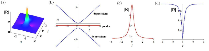
Figure 2: (color online). (a) The first-order rogue wave solution $\widetilde{R}_{2}(n,t)$ given by Eq. (31) with one peak and two depression points. (b) The motion of the peak and depression centers, as per Eqs. (33) and (34). Other panels display the evolution of the absolute value of the field at (c) the quiescent peak ($n=-\frac{2}{3}$) and (d) the moving depression points ($n=-\frac{2}{3}\pm\frac{1}{48}\sqrt{1344+6075t^{2}}$).

Figure 3: (color online). (a) The first-order rogue wave solution $\widetilde{S}_{2}(n,t)$ given by Eq. (31) with one peak and two depression points. (b) The motion of the peak and depression centers as per Eqs. (36) and (37). Other panels display the evolution of the absolute value of the field at (c) the quiescent peak ($n=-\frac{7}{6}$) and (d) the moving depression points ($n=-\frac{7}{6}\pm\frac{1}{48}\sqrt{1344+6075t^{2}}$).

$$\begin{array}[]{ll}|\widetilde{R}_{2}(n,t)|^{2}=\dfrac{9}{16}\dfrac{(2025t^{2}+2304n^{2}+3072n-320)^{2}+3600^{2}t^{2}}{(2025t^{2}+2304n^{2}+3072n+1280)^{2}},\vspace{0.1in}&\\ |\widetilde{S}_{2}(n,t)|^{2}=\dfrac{9}{16}\dfrac{(2025t^{2}+2304n^{2}+5376n+1792)^{2}+3600^{2}t^{2}}{(2025t^{2}+2304n^{2}+5376n+3392)^{2}},&\end{array}$$ (32)

As follows from here, $|\widetilde{R}_{2}(n,t)|^{2}$ has three critical points: $(n_{1},t_{1})=(-\frac{2}{3},0),(n_{2,3},t_{2,3})=(-\frac{4\pm\sqrt{21}}{6},0).$ The first point, $(n_{1},t_{1})$, is a maximum (peak), at which $|\widetilde{R}_{2,\max}(n,t)|=\frac{63}{16}$. The two other critical points $(n_{2,3},t_{2,3})$ are minima (depressions), at which the amplitude vanishes. Further, the (modulationally unstable) background value is given by $|\widetilde{R}_{2}(n,t)|\longrightarrow|\widetilde{R}_{2,\infty}(n,t)|=\frac{3}{4}$ at $|n|,t\longrightarrow\infty$. Thus, we find a relation between the peak and background values: $|\widetilde{R}_{2,\max}(n,t)|=\frac{21}{4}|\widetilde{R}_{2,\infty}(n,t)|$ (see Fig. 2(a)). Moreover, we have the conservation law $\int\limits_{-\infty}^{+\infty}(|\widetilde{R}_{2}(n,t)|^{2}-\frac{9}{16})dn=0$, which follows from the fact that the RW is actually formed from the flat background.

Next, intensity $|\widetilde{S}_{2}(n,t)|^{2}$ has three critical points: $(n_{1},t_{1})=(-\frac{7}{6},0),(n_{2,3},t_{2,3})=(-\frac{7\pm\sqrt{21}}{6},0),$ the first again being a maximum point (peak), with the corresponding maximum amplitude $|\widetilde{S}_{2,\max}(n,t)|=\frac{63}{16}$. Two other critical points, $(n_{2,3},t_{2,3})$, are minima (depressions), with zero amplitude. In this component, the background value is $|\widetilde{S}_{2}(n,t)|\longrightarrow|\widetilde{S}_{2,\infty}(n,t)|=\frac{3}{4}$ at $|n|,t\longrightarrow\infty$. Therefore, we have, as in the $\widetilde{R}_{2}$ component, $|\widetilde{S}_{2,\max}(n,t)|=\frac{21}{4}|\widetilde{S}_{2,\infty}(n,t)|$ (see Fig. 3(a)), and the respective conservation law, $\int\limits_{-\infty}^{+\infty}(|\widetilde{S}_{2}(n,t)|^{2}-\frac{9}{16})dn=0$.

For intensity $|\widetilde{R}_{2}(n,t)|^{2}$ given by Eq. (32), the trajectory of the peak’s centers is produced by the dependence of its spatial coordinate, $T_{rh}$, on $t$. It follows from the expression for $|\widetilde{R}_{2}(n,t)|^{2}$ that this coordinate actually stays constant,

$$\begin{array}[]{ll}T_{rh}=-\dfrac{2}{3},&\end{array}$$ (33)

while the coordinates, $T_{rc\pm}$, of centers of the two depressions are given by

$$\begin{array}[]{ll}T_{rc\pm}=-\dfrac{2}{3}\pm\dfrac{1}{48}\sqrt{6075t^{2}+1344}.&\end{array}$$ (34)

The comparison of Eqs. (33) and (34) produces the RW width, which is defined as the distance between the two depressions:

$$\begin{array}[]{ll}T_{rd}=\dfrac{1}{24}\sqrt{6075t^{2}+1344}.&\end{array}$$ (35)

Figure 2(b) displays the trajectories of the peak’s centers, $T_{rh}$, and centers of the two depressions, $T_{rc\pm}$. Figures 2(c) and 2(d) display profiles of $|\widetilde{R}_{2}(n,t)|$ at the peak ($n=-\frac{2}{3}$, as given by Eq. (33)) and depressions ($n=-\frac{2}{3}\pm\frac{1}{48}\sqrt{6075t^{2}+1344}$, as given by Eq. (34)).

For intensity $|\widetilde{S}_{2}(n,t)|^{2}$ given by Eq. (32), the trajectory of the peak’s centers is determined by the dependence of its spatial coordinate, $T_{sh}$, on $t$. It follows from the expression for $|\widetilde{S}_{2}(n,t)|^{2}$ that

$$\begin{array}[]{ll}T_{sh}=-\dfrac{7}{6},&\end{array}$$ (36)

and the spatial coordinates, $T_{sc\pm}$, of centers of the two depressions are given by

$$\begin{array}[]{ll}T_{sc\pm}=-\dfrac{7}{6}\pm\dfrac{1}{48}\sqrt{6075t^{2}+1344},&\end{array}$$ (37)

leading to the RW width, which is again defined as the spatial distance between two depressions:

$$\begin{array}[]{ll}T_{sd}=\dfrac{1}{24}\sqrt{6075t^{2}+1344},&\end{array}$$ (38)

Figure 3(b) displays the trajectories of the peak’s centers, $T_{sh}$, and of the centers of the two depressions, $T_{sc\pm}$. Figures 3(c) and 3(d) illustrate the profiles of $|\widetilde{R}_{2}(n,t)|$ at the peak ($n=-\frac{7}{6}$, as given by Eq. (36)) and depressions ($n=-\frac{7}{6}\pm\frac{1}{48}\sqrt{6075t^{2}+1344}$, as given by Eq. (37)).

In addition, it is relevant to note that the amplitude $c$ of the CW background can control the first-order RW solution (30) with $N=2$. Here we use values of $c$ to modulate the shape, central position, and amplitude of the first-order RW solution (see Figs. 4 and 5).

• For $c=\frac{5}{12}$ (i.e., $\lambda=\frac{9}{4}$), $\widetilde{R}_{2}(n,t)$ peaks around the point $(n_{1},t_{1})=(-\frac{9}{10},0)$, and the background value is determined by $|\widetilde{R}_{2}(n,t)|\longrightarrow|\widetilde{R}_{2,\infty}(n,t)|=\frac{5}{12}$ at $n,t\longrightarrow\infty$. The maximum value $|\widetilde{R}_{2,\max}(n,t)|$ of $|\widetilde{R}_{2}(n,t)|$ is $\frac{665}{432}$ at point $(n_{1},t_{1})=(-\frac{9}{10},0),$ and the minimum is zero, at $(n_{2,3},t_{2,3})=(-\frac{9\pm\sqrt{133}}{10},0)$, see Figs. 4a1-a2;

• When $c=1$ (i.e., $\lambda=3+2\sqrt{2}$), $\widetilde{R}_{2}(n,t)$ peaks around the point $(n_{1},t_{1})=(-\frac{1+\sqrt{2}}{4},0)$, and the background corresponds to $|\widetilde{R}_{2}(n,t)|\longrightarrow|\widetilde{R}_{2,\infty}(n,t)|=1$ at $n,t\longrightarrow\infty$. The maximum value $|\widetilde{R}_{2,\max}(n,t)|$ of $|\widetilde{R}_{2}(n,t)|$ is $7$ at $(n_{1},t_{1})=(-\frac{1+\sqrt{2}}{4},0)$, and the minimum is zero at $(n_{2,3},t_{2,3})=(-\frac{1+\sqrt{2}\pm\sqrt{7}}{4},0)$, see Figs. 4(b1-b2);

• For $c=\frac{4}{3}$ (i.e., $\lambda=9$), $\widetilde{R}_{2}(n,t)$ peaks around the point $(n_{1},t_{1})=(-\frac{9}{16},0)$, with the background corresponding to $|\widetilde{R}_{2}(n,t)|\longrightarrow|\widetilde{R}_{2,\infty}(n,t)|=\frac{4}{3}$ at $n,t\longrightarrow\infty$. The maximum value $|\widetilde{R}_{2,\max}(n,t)|$ of $|\widetilde{R}_{2}(n,t)|$ is $\frac{364}{27}$ at $(n_{1},t_{1})=(-\frac{9}{16},0)$ and the minimum value is again zero, at $(n_{2,3},t_{2,3})=(-\frac{9\pm\sqrt{91}}{16},0)$, see Figs. 4(c1-c2);

• When $c=\frac{12}{5}$ (i.e., $\lambda=25$), $\widetilde{R}_{2}(n,t)$ peaks around the point $(n_{1},t_{1})=(-\frac{25}{48},0)$, and the background corresponds to $|\widetilde{R}_{2}(n,t)|\longrightarrow|\widetilde{R}_{2,\infty}(n,t)|=\frac{12}{5}$ at $n,t\longrightarrow\infty$. The maximum value $|\widetilde{R}_{2,\max}(n,t)|$ of $|\widetilde{R}_{2}(n,t)|$ is $\frac{7812}{125}$ at $(n_{1},t_{1})=(-\frac{25}{48},0)$, and the minimum is, once again, zero, at $(n_{2,3},t_{2,3})=(-\frac{25\pm\sqrt{651}}{48},0)$, see Figs. 4(d1-d2).

From the above analysis, we conclude that the increase of spectral parameter $\lambda$ corresponds to the increase of $c$, and the amplitude of the first-order RW grows too with the increase of $c$. The central position and peak of the first-order RW move to the right along line $t=0$. A similarly picture is produced by the consideration of the other component.

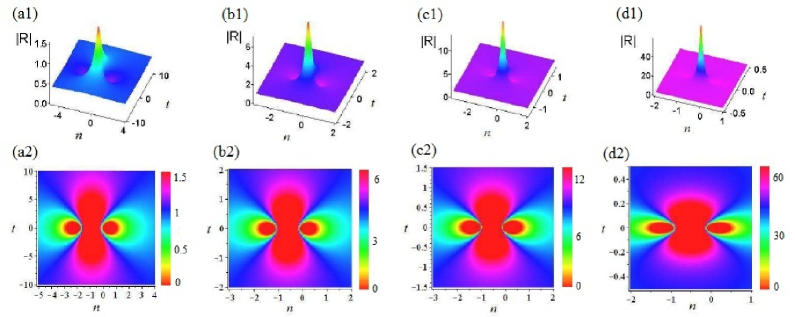
Figure 4: (color online). The first-order rogue-wave solution $\widetilde{R}_{2}(n,t)$, given by Eq. (30) with $N=2$: (a1)-(a2) $c=\frac{5}{12}$ (i.e., $\lambda=\frac{9}{4}$); (b1)-(b2) $c=1$ (i.e., $\lambda=3+2\sqrt{2}$); (c1)-(c2) $c=\frac{4}{3}$ (i.e., $\lambda=9$); and (d1)-(d2) $c=\frac{12}{5}$ (i.e., $\lambda=25$). In this figure and similar figures following below, the bottom row shows the top view of the generated RWs (note the difference in the scale of variable $t$ in comparison with the 3D plots displayed in the top row). In other figures showing top views, the color-code bar is the same as used here.

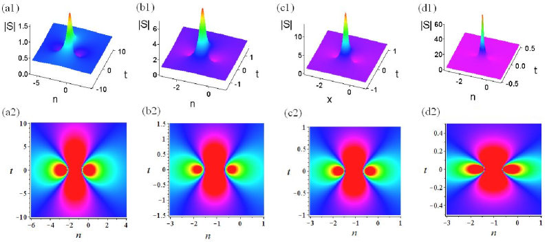
Figure 5: (color online). The first-order rogue wave solution $\widetilde{S}_{2}(n,t)$ given by Eq. (30) with $N=2$: (a1)-(a2) $c=\frac{5}{12}$ (i.e., $\lambda=\frac{9}{4}$); (b1)-(b2) $c=1$ (i.e., $\lambda=3+2\sqrt{2}$); (c1)-(c2) $c=\frac{4}{3}$ (i.e., $\lambda=9$); and (d1)-(d2) $c=\frac{12}{5}$ (i.e., $\lambda=25$).

Dynamical behavior—. To further study the wave propagation in the framework of the above discrete RW solutions, we here compare the exact solutions and their perturbed counterparts, produced by numerical simulations of Eq. (1) with the initial conditions given by these solutions with small perturbations.

Figure 6 exhibits the exact first-order RW solution, $\widetilde{R}_{2}(n,t)$ and $\widetilde{S}_{2}(n,t)$, as given by Eq. (32), and the one perturbed by small noise with amplitude $0.02$. Figures 4(a1)-(a2) and (b1)-(b2) show that the time evolution of the RW without the addition of the perturbation is very close to the corresponding exact RW solution (32) in a short time interval, $t\in(-2.5,2.5)$. However, if the small random noise is added to the initial condition (i.e., the RW solution (32) taken at $t=-2.5$), then the evolution exhibits weak perturbations at $t<2.5$, and conspicuous perturbations later, see Figs. 6(c1-c2).

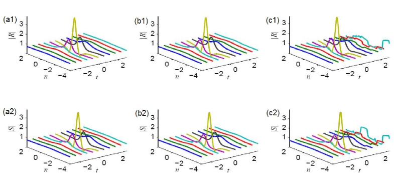
Figure 6: (color online). First-order RW solutions (32). The exact solution (left); the evolution generated by simulations using exact solutions (32) as an initial conditions (middle); and the evolution generated by adding random noise with amplitude ${\small 0.02}$ to the initial conditions (right).

IV.2 Second-order vector rogue waves

The structure of the second-order RWs—. Theorem 2 with $N=3$ produces the second-order vector RW solution of Eq. (1)

$$\widetilde{R}_{3}(n,t)=\dfrac{R_{0}(n,t)+{b_{n}^{(2)}}^{\ast}}{a_{n}^{(0)}}=\dfrac{3A_{1}(n,t)}{4B_{1}(n,t)}e^{\frac{25}{8}it},\,\,\,\widetilde{S}_{3}(n,t)={b_{n+1}^{(0)}+S_{0}(n,t)a_{n+1}^{(0)}}=\dfrac{3A_{2}(n,t)}{4B_{2}(n,t)}e^{-\frac{25}{8}it},$$ (39)

where $A_{j},B_{j}\,(j=1,2)$ are given by the following complex expressions:

$$\begin{array}[]{rl}A_{1}(n,t)=&16986931200tn^{3}+95551488000itd_{1}n^{2}-74649600000t^{2}d_{1}+59719680000it^{2}e_{1}\\ &-96259276800ine_{1}-4039114752in^{2}+3149280000it^{4}n^{2}-24286003200it^{2}n\\ &-67947724800in^{2}e_{1}-33973862400in^{3}e_{1}-27993600000it^{3}d_{1}+212336640000ie_{1}^{2}\\ &+3583180800it^{2}n^{4}-11346739200in^{2}t^{2}+53084160000itd_{1}+4199040000it^{4}n\\ &+9555148800it^{2}n^{3}+4920750000t^{5}+1358954496in^{6}+150994944in^{3}\\ &+127401984000itnd_{1}+5435817984in^{5}+212336640000id_{1}^{2}+26214400i\\ &+922640625it^{6}+14929920000nt^{3}-11943936000it^{2}-6488064000t\\ &-2390753280in+6370099200n^{2}t+47185920000d_{1}+6220800000t^{3}\\ &+84934656000n^{2}d_{1}+11197440000n^{2}t^{3}+6370099200n^{4}t-4811400000it^{4}\\ &+6002049024in^{4}+113246208000nd_{1}+106168320000te_{1}+159252480000nte_{1}\\ &-7785676800nt-47185920000ie_{1}+89579520000it^{2}ne_{1},\end{array}$$

$$\begin{array}[]{rl}B_{1}(n,t)=&-25480396800ne_{1}-4379443200nt^{2}+3583180800n^{2}t^{2}+5435817984n^{5}\\ &+1358954496n^{6}+2013265920n+127401984000ntd_{1}+9555148800n^{3}t^{2}\\ &+3149280000n^{2}t^{4}+89579520000nt^{2}e_{1}+4199040000nt^{4}-33973862400n^{3}e_{1}\\ &+3583180800n^{4}t^{2}+95551488000n^{2}td_{1}+1534464000t^{2}+6123600000t^{4}\\ &-13271040000td_{1}+212336640000e_{1}^{2}+212336640000d_{1}^{2}+922640625t^{6}\\ &-27993600000t^{3}d_{1}+59719680000t^{2}e_{1}+4690280448n^{2}+7700742144n^{3}\\ &+8833204224n^{4}-67947724800n^{2}e_{1}+419430400,\end{array}$$

$$\begin{array}[]{rl}A_{2}(n,t)=&-118908518400ne_{1}+8161689600nt^{2}+23290675200n^{2}t^{2}+9512681472n^{5}\\ &+1358954496n^{6}+4304404480+18849202176n+222953472000ntd_{1}\\ &+16721510400n^{3}t^{2}+3149280000n^{2}t^{4}+89579520000nt^{2}e_{1}+7348320000nt^{4}\\ &-33973862400n^{3}e_{1}-33973862400e_{1}+3583180800n^{4}t^{2}+95551488000n^{2}td_{1}\\ &+1658880000t^{2}+9010440000t^{4}+74317824000td_{1}+212336640000e_{1}^{2}\\ &+212336640000d_{1}^{2}+922640625t^{6}-27993600000t^{3}d_{1}+104509440000t^{2}e_{1}\\ &+37559992320n^{2}+42354081792n^{3}+27518828544n^{4}-118908518400n^{2}e_{1}.\\ &\end{array}\qquad\quad$$

$$\begin{array}[]{rl}B_{2}(n,t)=&-29727129600tn^{3}+104509440000it^{2}e_{1}+222953472000itnd_{1}+89579520000it^{2}ne_{1}\\ &-26674790400it^{2}n-25505280000it^{2}+95551488000itd_{1}n^{2}+74649600000t^{2}d_{1}\\ &+24687673344in^{4}-189687398400ine_{1}-1362100224in+140673024000itd_{1}\\ &-118908518400in^{2}e_{1}+16721510400it^{2}n^{3}+3583180800it^{2}n^{4}\\ &-33973862400in^{3}e_{1}+13259243520in^{2}+7348320000it^{4}n+3149280000it^{4}n^{2}\\ &+9512681472in^{5}+29142024192in^{3}-116549222400ie_{1}-27993600000it^{3}d_{1}\\ &-1924560000it^{4}-4920750000t^{5}+1358954496in^{6}+922640625it^{6}-1593835520i\\ &+8360755200in^{2}t^{2}-26127360000nt^{3}+212336640000ie_{1}^{2}+6266880000t\\ &-41405644800n^{2}t-125042688000d_{1}-16485120000t^{3}+212336640000id_{1}^{2}\\ &-84934656000n^{2}d_{1}-11197440000n^{2}t^{3}-6370099200n^{4}t-198180864000nd_{1}\\ &-185794560000te_{1}-159252480000nte_{1}-14509670400nt,\end{array}$$

The profiles of the second-order RW solutions (39) are displayed in Figs. 7 and 8. The pair of introduced parameters $e_{1}$ and $d_{1}$ can be used to control strong and weak interactions of the second-order RW solutions (39), by which we mean, respectively, tightly and loosely bound patterns:

• For $e_{1}=d_{1}=0$, we observe the strong interaction, see Figs. 7(a,b) and Figs. 8(a,b), which exhibit five local maxima (peaks) and four minima (holes).

• For $e_{1}d_{1}\neq 0$, we observe the weak interaction, see Figs. 7(c)-(d) and Figs. 8(c)-(d), in which the second-order RW is split into three first-order RWs, whose centers form a rotating triangle, and there are three local maxima (peaks) and six minima (holes) exhibited by every profile. Moreover, we find that the size of the triangle increase with the increase of $|e_{1}|$ or $|d_{1}|$, and $d_{1}$ controls the rotation of the triangle profile. When both $|e_{1}|$ and $|d_{1}|$ drop to zero, the three split first-order RWs feature strong interaction (cf. Figs. 7(c)-(d) or 8(c)-(d) and Figs. 7(a)-(b) or 8(a)-(b)), and the local maxima grow, while the minimum values decrease, which is an effect of the strong interaction between the first-order RWs. We do not report here the dependence of the angular velocity of the rotation on the system’s parameters, as this analysis requires extremely heavy simulations.

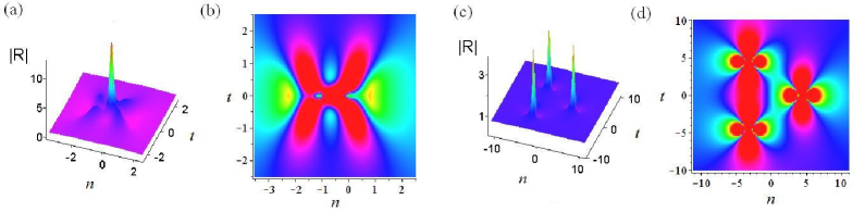
Figure 7: (color online). The second-order RW solution $\widetilde{R}_{3}(n,t)$ given by Eq. (39): (a)-(b) $e_{1}=d_{1}=0$; (c)-(d) – a triangular pattern with $e_{1}=10,d_{1}=0$.

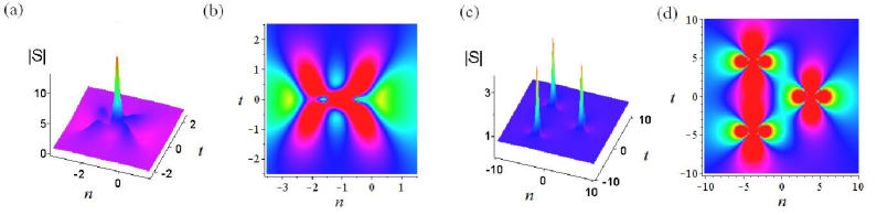
Figure 8: (color online). The second-order RW solution $\widetilde{S}_{3}(n,t)$ given by Eq. (39): (a)-(b) $e_{1}=d_{1}=0$; (c)-(d) – a triangular pattern with $e_{1}=10,d_{1}=0$.

Dynamical behavior—. Next, we study the dynamical behavior of the second-order RWs, $\widetilde{R}_{3}(n,t)$ and $\widetilde{S}_{3}(n,t)$, given by Eq. (39), by means of numerical simulations. We consider cases of the strong (Figs. 7(a) and  8(a)) and weak (Figs. 7c and  8c) interaction. Figures 9(b1)-(b2) and (a1)-(a2) show that the evolution of the second-order RW solution $\widetilde{R}_{3}(n,t)$ in the regime of the strong interaction without the addition of noise almost exactly corroborates the corresponding exact RW solution (39), in the time interval $t\in(-2.5,\,2.5)$. If random noise with amplitude $0.05$ (which is larger than the noise amplitude considered above) is added to the initial condition, taken as per RW solution (39) with $e_{1}=d_{1}=0$ at $t=-2.5$, then the evolution exhibits only relatively small perturbations, in comparison with the unperturbed solution, see Figs. 9(c1)-(c2).

However, in the case of the weak interaction (see Figs. 7(c) and  8(c)) the results are different. The second-order RW solution (39) exhibits perturbations at $t>0$ even without adding the noise to the initial conditions, which indicates strong instability of the RW solution in this case, see Figs. 10(b1)-(b2). If really weak random noise , with amplitude $0.01$, is added to the initial solution, i.e., to RW (39) with $e_{1}=10,\,d_{1}=0$ at $t=-8$, the simulated evolution exhibits obviously strong instability at $t>0$, see Figs. 10(c1)-(c2).

Thus, Figs. 9(c1)-(c2) and  10(c1)-(c2) demonstrate that the weak random noise produces a weak (strong) effect in the case of the strong (weak) interaction. The difference may be explained by the fact that, in the former case (strong interaction), the energy is concentrated close to the origin in $(n,t)$ plane, see Figs. 9(a1)-(a2), while in the latter case (weak interaction) case the energy is spread around three points in the $(n,t)$ plane, see Figs. 10(a1)-(a2), making this loosely bound pattern more amenable to perturbation effects.

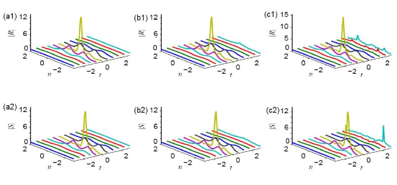
Figure 9: (color online). The second-order RW solutions (39) with $e_{1}=d_{1}=0$. The exact solution (left), the simulated evolution using the exact solutions (39) as the initial conditions (middle), and the evolution initiated by the exact solution perturbed by relatively strong random noise with amplitude ${\small 0.05}$.

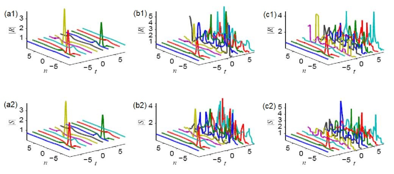
Figure 10: (color online). The second-order RW solutions (39) with $e_{1}=10,d_{1}=0$. The exact solution (left), simulated evolution with the exact solution (39) used as the initial conditions (middle), and the evolution initiated by the exact solutions perturbed by weak random noise with amplitude ${\small 0.01}$.

IV.3 Third-order vector rogue waves

The structure of the third-order RWs—. Theorem 2 with $N=4$ produces the third-order vector RW solution of Eq. (1):

$$\widetilde{R}_{4}(n,t)=\dfrac{R_{0}(n,t)+{b_{n}^{(3)}}^{\ast}}{a_{n}^{(0)}},\ \ \ \widetilde{S}_{4}(n,t)={b_{n+1}^{(0)}+S_{0}(n,t)a_{n+1}^{(0)}}.$$ (40)

An explicit analytical expression for this solution is not written here, as it is very cumbersome. Variation of control parameters $e_{1},\,e_{2},\,d_{1},\,d_{2}$ casts the third-order RW into different forms.

• At $e_{1,2}=d_{1,2}=0$, the third-order exists in the regime of strong interaction, with the corresponding density graphs displayed in Figs. 11(a1)-(a2) and 12(a1)-(a2).

• At $e_{1}=10,\,d_{1,2}=e_{2}=0$, the weak interaction allows splitting of the third-order RW into six first-order RWs, which form a triangular pattern, see Figs. 11(b1)-(b2) and 12(b1)-(b2).

• At $e_{2}=100,\,d_{1,2}=e_{2}=0$, the weak interaction in the third-order RW also leads to splitting into six first-order RWs, which form a rotating pentagon pattern with a first-order RW located near the center, see Figs. 11(c1)-(c2) and 12(c1)-(c2).

• If we choose one nonzero parameter in each sets $\{e_{1},d_{1}\}$ and $\{e_{2},\,d_{2}\}$ (e.g., $e_{1}=17.6875,e_{2}=230,d_{1,2}=0$), then the third-order RW solution (40) displays a different quadrangle pattern, that is, a second-order RW with the highest peak on the right side, and three first-order RWs that form an arc on the left side, see Figs. 11(c1)-(c2) and 12(c1)-(c2).

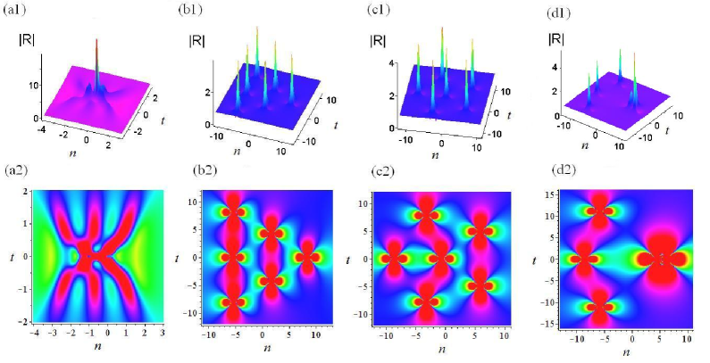
Figure 11: (color online). The third-order RW solution $\widetilde{R}_{4}(n,t)$ given by Eq. (40): (a1)-(a2) $e_{1,2}=d_{1,2}=0$; (b1)-(b2) – a triangular pattern with $e_{1}=10,d_{1,2}=e_{2}=0$; (c1)-(c2) – a pentagon pattern with $e_{2}=100,e_{1}=d_{1,2}=0$; and (d1)-(d2) display a quadrangle pattern with $e_{1}=17.6875,e_{2}=230,d_{1,2}=0$.

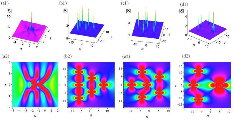
Figure 12: (color online). The third-order RW solution $\widetilde{S}_{4}(n,t)$ given by Eq. (40): (a1)-(a2) $e_{1,2}=d_{1,2}=0$; (b1)-(b2) – a triangular pattern with $e_{1}=10,d_{1,2}=e_{2}=0$; (c1)-(c2) – a pentagon pattern with $e_{2}=100,e_{1}=d_{1,2}=0$; and (d1)-(d2) display a quadrangle pattern with $e_{1}=17.6875,e_{2}=230,d_{1,2}=0$.

Dynamical behavior—. We proceed to simulations of the evolution of the third-order RW solutions $\widetilde{R}_{4}(n,t)$ and $\widetilde{S}_{4}(n,t)$ given by Eq. (40). We again consider regimes of the strong and weak interaction, for which Figs. 13-15(a1) and (a2), respectively, show that the unperturbed evolution agrees with the corresponding exact solutions (40) in a short time interval. At $t>0$, the solution corresponding to the weak interaction (Figs. 11(b1,c1) and Figs. 12(b1,c1)) exhibits growing perturbations even in the absence of the initially added random noise, which indicates instability (see Figs. 13-15(b1) and (b2)). This may be explained, as above, by the fact that to the energy is spread in a larger domain, in comparison with ones in Fig. 11(a1) and Fig. 12(a1). If weak random noise, with amplitude $0.01$, is added to the initial conditions, see Figs. 11 and 12(a1,b1,c1), then the evolution of the third-order RW solution in the weak-interaction regime exhibits strong instability, while the perturbation growth is much slower in the strong-interaction regime, see Fig. 11(a1) and Fig. 12(a1). Once again, these results may be explained by the concentration of the energy around the origin in the $\left(n,t\right)$ plane under the action of the strong interaction, see Figs. 13-15(a1), and by the spread of the energy around several points in the case of the weak interaction, see Figs. 13-15(b1,c1).

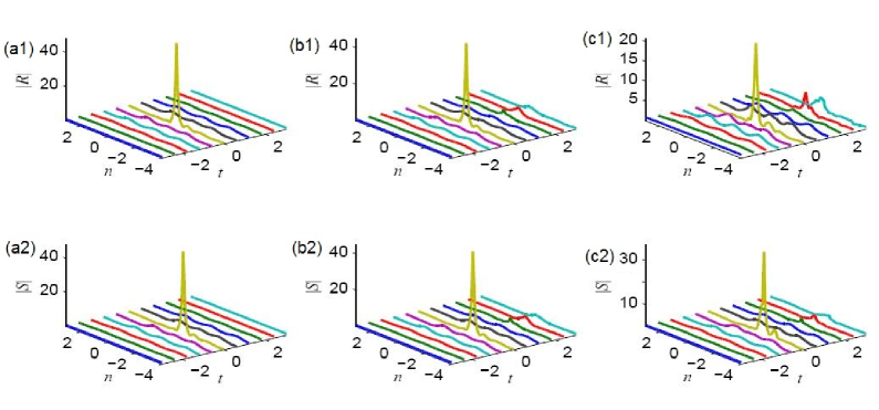
Figure 13: (color online). The third-order RW solutions (40) with $e_{1,2}=d_{1,2}=0$. The exact solution (left); simulated evolution using exact solutions (40) as the initial conditions (middle); and the evolution initiated by the exact solutions perturbed by relatively strong random noise with amplitude ${\small 0.08}$ (right).

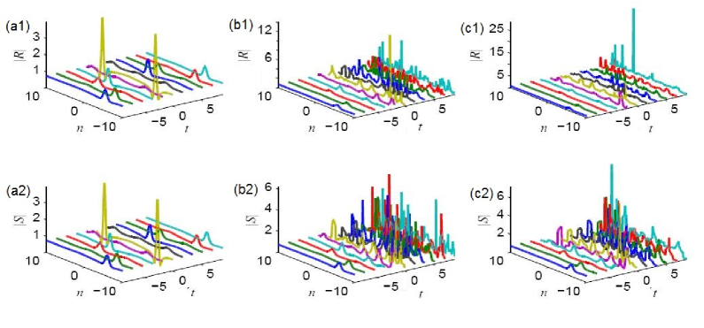
Figure 14: (color online). The third-order RW solutions (40) with $e_{1}=10,d_{1,2}=e_{2}=0$. The exact solution (left); simulated evolution using exact solutions (40) as the initial conditions (middle); the evolution initiated by the exact solution perturbed by weak random noise with amplitude ${\small 0.01}$ (right).

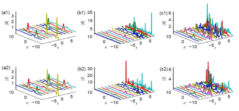
Figure 15: (color online). The third-order RW solutions (40) with $e_{2}=100,d_{1,2}=e_{1}=0$. The exact solution (left); simulated evolution using exact solutions (40) as the initial condition (middle); the evolution initiated by the exact solution perturbed by weak random noise with amplitude ${\small 0.01}$ (right).

Similarly, Theorem 2 with $N>4$ produces the higher-order RW solution of Eq. (1), which can also generate the abundant discrete wave structures.

V Conclusion

The subject of this work is the construction of families of higher-order discrete RW (rogue-wave) states, which can be found in the integrable system of coupled AL (Ablowitz-Ladik) equations. These equations may serve as models for the dynamics of BEC trapped in a deep optical lattice. In the work, we have presented a novel method for constructing generalized $(M,N-M)$-fold Darboux transforms (DTs) of the coupled AL system, which is based on the fractional form of the respective determinants. Then, we apply the generalized $(1,N-1)$-fold DTs to produce higher-order RW solutions. They display a variety of patterns, including the rotating triangles and pentagons, as well as quadrangle structures, which represent multi-RWs in the system, and suggest shapes which such higher-order RW may assume in other physically relevant models. The evolutions of the multi-RW solutions was studied by means of systematic simulations, which demonstrate that the tightly and loosely bound solutions are, respectively, nearly stable and strongly unstable ones.

As an extension of this work, it may be interesting to look for similar complex RW modes, by means of numerical methods, in more generic nonintegrable discrete systems.

Acknowledgments

The authors would like to thank the anonymous referees for their valuable comments and suggestions which help to improve the manuscript. This work has been partially supported by the NSFC under Grants Nos. 11375030 and 11571346, and China Postdoctoral Science Foundation under Grant No. 2015M570161.

Appendix A
Explicit expressions for functions $\left\{\phi^{(2,3)}\right\}$ and $\left\{\psi^{(2,3)}\right\}$ in Eq. (29):
$\phi^{(2)}=-\frac{1}{78643200}(\frac{25}{16})^{n}e^{-\frac{55}{16}it}(55296000itd_{1}+49152000ie_{1}-20697600it^{2}+1966080in^{3}-2621440in-16934400int^{2}+589824in^{2}+455625it^{4}+58982400ine_{1}+589824in^{4}-3110400in^{2}t^{2}-819200i+3276800t+16711680nt+2211840tn^{3}-58982400nd_{1}-1944000nt^{3}+55296000te_{1}+11796480n^{2}t-7128000t^{3}-49152000d_{1}),$

$\psi^{(2)}=-\frac{1}{13107200}(\frac{25}{16})^{n}e^{-\frac{5}{16}it}(-102400it+18432000ite_{1}-19660800ne_{1}+737280itn^{3}+3916800nt^{2}-648000int^{3}+2088960in^{2}t+3347200t^{2}+1474560itn-18432000td_{1}-19660800ind_{1}-151875t^{4}+131072n^{2}-196608n^{4}-1836000it^{3}+1036800n^{2}t^{2}),$

$\phi^{(3)}=-\frac{1}{1006632960000}(\frac{25}{16})^{n}e^{-\frac{55}{16}it}(754974720000ine_{2}+20447232000tn^{3}+541900800000t^{2}d_{1}\newline +212336640000in^{2}td_{1}+150994944in^{6}-199065600000int^{2}e_{1}-943718400000id_{1}^{2}+754974720in^{5}+754974720000intd_{1}+125829120in^{4}-17838080000it^{2}-4194304000in^{3}+188743680000in^{2}e_{1}+5326766080in+943718400000ie_{1}^{2}+3645000000t^{5}+629145600000ie_{2}+707788800000itd_{2}+2621440000i-3841982464in^{2}-93035520000nt^{3}-10485760000t+7549747200n^{2}t+150994944000ine_{1}-10485760000d_{1}-629145600000d_{2}+640942080000itd_{1}+75497472000in^{3}e_{1}-21676032000in^{3}t^{2}-541900800000it^{2}e_{1}-92318720000t^{3}-62208000000it^{3}d_{1}-78151680000in^{2}t^{2}-75497472000n^{3}d_{1}-754974720000nd_{2}-188743680000n^{2}d_{1}-27371520000n^{2}t^{3}+656100000nt^{5}+849346560tn^{5}+707788800000te_{2}+16135200000int^{4}+35283600000it^{4}-102515625it^{6}-62208000000t^{3}e_{1}-1887436800000e_{1}d_{1}-2488320000n^{3}t^{3}+7549747200n^{4}t-150994944000nd_{1}+640942080000te_{1}+754974720000nte_{1}+199065600000nt^{2}d_{1}+212336640000n^{2}te_{1}-95821824000int^{2}+1749600000in^{2}t^{4}-27561820160nt-1990656000in^{4}t^{2}+10485760000ie_{1}),$

$\psi^{(3)}=-\frac{1}{503316480000}(\frac{25}{16})^{n}e^{-\frac{5}{16}it}(-88080384000ne_{1}+27869184000nt^{2}+37232640000n^{2}t^{2}-42091520000it^{3}-150994944n^{6}+3098250000it^{5}-1887436800000ie_{1}d_{1}+376012800000it^{2}d_{1}-88080384000ind_{1}+401080320000inte_{1}+199065600000int^{2}d_{1}+212336640000in^{2}te_{1}-401080320000ntd_{1}+15040512000n^{3}t^{2}+707788800000ite_{2}-1749600000n^{2}t^{4}-754974720000ne_{2}+199065600000nt^{2}e_{1}-13219200000nt^{4}-75497472000n^{3}e_{1}+4010803200in^{4}t-3853516800in^{2}t+4718592000itn^{3}-754974720000ind_{2}+1990656000n^{4}t^{2}-212336640000n^{2}td_{1}-2488320000in^{3}t^{3}+656100000int^{5}-55710720000int^{3}-62208000000it^{3}e_{1}+849346560itn^{5}+247726080000ite_{1}-21150720000in^{2}t^{3}-75497472000in^{3}d_{1}+983040000it-798720000t^{2}-23781600000t^{4}-247726080000td_{1}-707788800000td_{2}-943718400000e_{1}^{2}+943718400000d_{1}^{2}+102515625t^{6}+62208000000t^{3}d_{1}+376012800000t^{2}e_{1}+276824064n^{2}+503316480n^{4}-6590300160itn).$

References

- (1) M. J. Ablowitz and P. A. Clarkson, Solitons, Nonlinear Evolution Equations and Inverse Scattering (Cambridge University Press, Cambridge, 1990).
- (2) L. Pitaevskii and S. Stringari, Bose-Einstein Condensation (Oxford University Press, Oxford, 2003).
- (3) V. S. Bagnato, D. J. Frantzeskakis, P. G. Kevrekidis, B. A. Malomed, and D. Mihalache, Rom. Rep. Phys. 67, 5 (2015).
- (4) J. M. Dudley, F. Dias, M. Erkintalo, and G. Genty, Nature Phys. 8, 755 (2014).
- (5) N. Akhmediev, B. Kibler, F. Baronio, M. Belić, W.-P. Zhong, Y. Zhang, W. Chang, J. M. Soto-Crespo, P. Vouzas, P. Grelu, C. Lecaplain, K. Hammani, S. Rica, A. Picozzi, M. Tlidi, K. Panajotov, A. Mussot, A. Bendahmane, P. Szriftgiser, G. Genty, J. Dudley, A. Kudlinski, A. Demircan, U. Morgner, S. Amiramashvili, C. Bree, G. Steinmeyer, C. Masoller, N. G. R. Broderick, A. F. J. Runge, M. Erkintalo, S. Residori, U. Bortolozzo, F. T. Arecchi, S. Wabnitz, C. G. Tiofack, S. Coulibaly, and M. Taki, Viewpoint, J. Optics 18, 063001 (2016).
- (6) B. A. Malomed, Nonlinear Schrödinger equations, in: Encyclopedia of Nonlinear Science, p. 639. Ed. A. Scott. New York: Routledge, 2005.
- (7) B. A. Malomed, D. Mihalache, F. Wise, and L. Torner, J. Optics B: Quant. Semicl. Opt. 7, R53-R72 (2005); B. A. Malomed, D. Mihalache, F. Wise, and L. Torner, Viewpoint, J. Phys. B: At. Mol. Opt. Phys. 49, 170502 (2016).
- (8) R. Carretero-González, D. J. Frantzeskakis, and P. G. Kevrekidis, Nonlinearity 21, R139 (2008).
- (9) Y. V. Kartashov, B. A. Malomed, and L. Torner, Rev. Mod. Phys. 83, 247 (2011).
- (10) W. X. Ma and M. Chen, Appl. Math. Comput. 215, 2835 (2009).
- (11) V. Ivancevic, Cognitive Computation 2, 17 (2010); e-print, arXiv:0911.1834.
- (12) Z. Yan, Commun. Theor. Phys. 54, 947 (2010); e-print, arXiv:0911.4295.
- (13) Z. Yan, Phys. Lett. A 375, 4274 (2011).
- (14) N. Akhmediev, J. M. Soto-Crespo, and A. Ankiewicz, Phys. Rev. A 80, 043818 (2009).
- (15) A. Ankiewicz, Y. Wang, S. Wabnitz, and N. Akhmediev, Phys. Rev. E 89, 012907 (2014).
- (16) Z. Yan, V. V. Konotop, and N. Akhmediev, Phys. Rev. E 82, 036610 (2010).
- (17) Z. Yan, Phys. Lett. A 374, 672 (2010).
- (18) B. L. Guo, L. M. Ling, Q. P. Liu, Phys. Rev. E 85, 026607 (2012).
- (19) S. Chen and D. Mihalache, J. Phys. A 48, 215202 (2015).
- (20) Y. Ohta and J. Yang, Phys. Rev. E 86, 036604 (2012).
- (21) X. Wen, Y. Yang, and Z. Yan, Phys. Rev. E 92, 012917 (2015).
- (22) X. Wen and Z. Yan, Chaos 25, 123115 (2015).
- (23) Y. Yang, Z. Yan, and B. A. Malomed, Chaos 25, 103112 (2015).
- (24) Z. Yan, Nonlinear Dyn. 79, 2515 (2015).
- (25) X. Y. Wen, Z. Yan, and Y. Yang, Chaos 26, 063123 (2016).
- (26) S. Chen, J. M. Soto-Crespo, F. Baronio, Ph. Grelu, and D. Mihalache, Opt. Express 24, 15251 (2016).
- (27) F. Yuan, J. Rao, K. Porsezian, D. Mihalache, and J. S. He, Rom. J. Phys. 61, 378 (2016).
- (28) M. J. Ablowitz and J. F. Ladik, J. Math. Phys. 16, 598 (1975).
- (29) A. Ankiewicz, N. Akhmediev, and J. M. Soto-Crespo, Phys. Rev. E 82, 026602 (2010).
- (30) A. Ankiewicz, N. Akhmediev, and F. Lederer, Phys. Rev. E 83, 056602 (2011).
- (31) Y. Ohta and J. Yang, J. Phys. A: Math. Theor. 47, 255201 (2014).
- (32) X. Y. Wen and Z. Yan, to be submitted (2016).
- (33) A. Szameit, F. Dreisow, M. Heinrich, S. Nolte, and A. A. Sukhorukov, Phys. Rev. Lett. 106, 193903 (2011).
- (34) O. Dutta, M. Gajda, P. Hauke, M. Lewenstein, D.-S. Luhmann, B. Malomed, T. Sowinski, and J. Zakrzewski, Rep. Prog. Phys. 78, 066001 (2015).
- (35) B. A. Malomed and J. Yang, Phys. Lett. A 302, 163 (2002).
- (36) X. Y. Wen, D. S. Wang and X. H. Meng, Rep. Math. Phys. 72, 349 (2013).
- (37) A. Ankiewicz, N. Devine, M. Ünal, A. Chowdury, and N. Akhmediev, J. Opt. 15, 064008 (2013).
- (38) X. Y. Wen, J. Phys. Soc. Jpn. 81, 114006 (2012).