Electric dipole moment of the neutron from
a flavor changing Higgs-boson

Abstract

I consider neutron electric dipole moment contributions induced by flavor changing Standard Model Higgs boson couplings to quarks. Such couplings might stem from non-renormalizable $SU(2)_{L}\times U(1)_{Y}$ invariant Lagrange terms of dimension six, containing a product of three Higgs doublets. Previously one loop diagrams with such couplings were considered in order to constrain quadratric expressions of Higgs flavor changing couplings to quarks. In the present paper the analysis is extended to the two loop level, where there are diagrams for electric dipole moments of quarks with a flavor changing Higgs coupling to first order only. The divergent loops, due to non-renormalisabillity, are parametrized in terms of an ultraviolet cut-off $\Lambda$. I also consider QCD corrections, including the mixing with the color electric dipole moment, while the contribution from the Weinberg operator is found to be negligible. The effect of QCD corrections is to suppress the bare result.

Using the current experimental bound on the neutron electric dipole moment, then for cut offs from one to seven TeV, I find a constraint of order $10^{-3}$ for the imaginary part of the product of the Higgs flavor changing coupling for $(d\rightarrow b)$-transition and the CKM element $V_{td}$. Assuming that the previous bound of the absolute value of the Higgs flavor changing coupling for $(d\rightarrow b)$-transition obtained from $B_{d}-\bar{B_{d}}$-mixing is saturated, the experimental bound on the neutron electric dipole moment would be reached for the bare result, if the cut off were extended up to about ca 20 TeV. However, QCD corrections suppress this result by a factor of order ten, and keep the nEDM below the experimental bound.

Keywords: CP-violation, Electric dipole moment, Flavor changing Higgs.
PACS: 12.15. Lk. , 12.60. Fr.

I Introduction

An electric dipole moment (EDM) for elementary particles is a CP-violating quantity and it gives important information on the matter anti-matter asymmetry in the universe. EDMs of elementary fermions within the Standard Model (SM) are induced through the Cabibbo-Kobayashi-Maskawa (CKM) CP-violating phase. EDMs are studied also within many models Beyond the SM (BSM). For reviews on SM and BSM EDMs, seePospelov:2005pr ; Fukuyama:2012np ; Dekens:2014jka ; Jung:2013hka ; Yamanaka:2017mef . Experimentally only bounds on electron, muon, proton and neutron EDMs are determined Olive:2016xmw . Explicitly, for the EDM of the neutron (nEDM $\equiv\,d_{n}$) discussed in this paper, the present experimental bound is Baker:2006ts

$$d_{n}^{exp}/e\leq 2.9\times 10^{-26}\,\mbox{cm}\;.$$ (1)

Within the SM, the nEDM is calculated to be several orders of magnitudes below the experimental bound. Calculations of the nEDM will in general put bounds on hypothetical models BSM, and any measured nEDM significantly bigger that the SM estimate ($10^{-32}$ to $10^{-31}\,e$ cm) would signal New Physics.

The SM contributions to the nEDM are well known and thoroughly explained in Pospelov:2005pr . At a low energy scale one can construct an effective Lagrangian

$${\cal L}_{\mathrm{eff}}\;=\;{\cal L}_{4}+{\cal L}_{5}+{\cal L}_{6}+...\,,$$ (2)

with all possible CP-odd operators of appropriate dimension. The QCD-odd term gives the dimension 4 operator Pospelov:2005pr ; Yamanaka:2017mef . The dimension 5 term contains electric dipole moment operators as well as color electric operators of quarks. The color electric operator and the the CP-odd three-gluon Weinberg operator (of dimension six) will in general mix under QCD renormakization Pospelov:2005pr ; Fukuyama:2012np ; Dekens:2014jka . The electric dipole moment of a single fermion in (2) has the form

$${\cal L}_{\mathrm{5,em}}\;=\;\frac{i}{2}\,d_{f}\,\bar{\psi_{f}}\sigma_{\mu\nu}\,F^{\mu\nu}\,\,\gamma_{5}\psi_{f}\;\;,$$ (3)

where $d_{f}$ is the electric dipolement of the fermion, $\psi_{f}$ is the fermion (quark) field, $F^{\mu\nu}$ is the electromagnetic field tensor, and $\sigma_{\mu\nu}=i[\gamma_{\mu},\,\gamma_{\nu}]/2$ is the dipole operator in Dirac space. The color electric dipole operator is given by the same expression with $d_{f}$ replaced by the color electric dipole moment $d^{c}_{f}$ and $F_{\mu\nu}$ replaced by $G^{a}_{\mu\nu}\,t^{a}$, where $G^{a}_{\mu\nu}$ is the color octet gluon tensor, and $t^{a}$ are the $SU(3)_{c}$ color matrices. The electric dipole operator in (3) for quarks appears within the SM from three loop diagrams with double Glashow-Iliopoulos-Maiani (GIM)- cancellations and in addition a gluon exchange. These are of order $\alpha_{s}G_{F}^{2}$, and are proportional to quark masses and an imaginary Cabibbo-Kobayashi-Maskawa(CKM) factor. They were found to be very small, of order $10^{-34}e$ cm Shabalin:1980tf ; Czarnecki:1997bu . Still within the SM, many contributions to the nEDM due to interplay of quarks in the neutron, were studied Pospelov:2005pr ; Maiezza:2014ala ; Nanopoulos:1979my ; Morel:1979ep ; Gavela:1981sk ; Khriplovich:1981ca ; McKellar:1987tf ; Eeg:1982qm ; Eeg:1983mt ; Hamzaoui:1985ri ; Mannel:2012qk . These mechanisms, gave results of order $10^{-33}$ to $10^{-31}e$ cm.

The nEDM due to EDMs of light $u$- and $d$-, and even $s$-quarks may be given by the formula

$$d_{n}\,=\,\rho_{u}\,d_{u}\;+\;\rho_{d}\,d_{d}\;+\;\rho_{s}\,d_{s}\;,$$ (4)

similar to a corresponding formula for the magnetic moment. In the strict valence approximation,

$$\rho_{u}\,=-\frac{1}{3}\;,\;\,\rho_{d}\,=\;\frac{4}{3}\;,\;\,\rho_{s}\,=0\;,$$ (5)

while lattice calculations Bhattacharya:2015esa ; Bhattacharya:2015wna give

$$\rho_{u}\,=-0.22\pm 0.03\;,\;\,\rho_{d}\,=\;0.74\pm 0.07\;,\;\,\rho_{s}\,=0.008\pm 0.010\;.$$ (6)

Note that there is a contribution to the nEDM from the EDM of the $s$-quark, with a small coefficient.

Many models BSM suggest possible new particles and/or new interaction Lagrange terms inducing EDMs Pospelov:2005pr ; Fukuyama:2012np ; Dekens:2014jka ; Jung:2013hka ; Yamanaka:2017mef ; Maiezza:2014ala ; Buchmuller:1982ye ; Manohar:2006ga ; Altmannshofer:2010ad ; Buras:2010zm ; Degrassi:2010ne ; Arnold:2012sd ; Brod:2013cka ; He:2014uya ; Fajer:2014ara ; Fuyuto:2015ida ; Bian:2016zba . In the case of New Physics (NP) presence, flavor physics might be testable through CP-violating asymmetries in mesonic decays Altmannshofer:2010ad ; Buras:2010zm ; Altmannshofer:2012ur . The properties and couplings of the physical Higgs boson ($H$) are still not completely known. Some authors Goudelis:2011un ; Blankenburg:2012ex ; Harnik:2012pb ; Greljo:2014dka ; Gorbahn:2014sha ; Dorsner:2015mja have suggested that the physical Higgs boson might have flavor changing couplings to fermions which might also be CP-violating. In these papers bounds on quadratic expressions of such couplings were obtained from various processes, say, like $K-\bar{K},\,D-\bar{D}\,$, and $B-\bar{B}$ - mixings, and also from leptonic flavor changing decays like $\mu\rightarrow e\,\gamma$ and $\tau\rightarrow\mu\,\gamma$. In the latter case two loop diagrams of Barr-Zee type Barr:1990vd were also considered Goudelis:2011un ; Blankenburg:2012ex ; Harnik:2012pb ; Chang:1993kw . (See also Leigh:1990kf ). Flavor changing couplings of this type will occur if the SM Higgs have non-renormalized interactions appearing when higher mass states are integrated out. For instance, flavor changing Higgs (FCH) couplings might stem from $SU(2)_{L}\times U(1)_{Y}$-invariant but non-renormalizable Lagrangian terms of dimension six.

The purpose of the present paper is to extend the analysis of Blankenburg:2012ex ; Harnik:2012pb to two loop diagrams. In the one loop case one needed two FCH couplings to generate the EDM. In the two loop case it is however possible to find diagrams with the FCH coupling to first order only, while the rest of the couplings are ordinary SM couplings.

Some of these two loop diagrams considered here give contributions suppressed by the small mass ratio $m_{d}/M_{W}$ for the ordinary SM Higgs coupling to fermions. ($M_{W}$ denotes the mass of the $W$-boson and $m_{q}$ is the mass of the quark $q$). However, if the Higgs is coupled to a top ($t$) quark one might obtain relevant non-suppressed contributions. Motivated by the result of the previous work Fajer:2014ara , I consider such diagrams. There are additional reasons to extend the analysis in Blankenburg:2012ex ; Harnik:2012pb for nEDM to two loop level. Namely, in general, it is known that some two loop diagrams might give bigger amplitudes than one loop diagrams because of helicity flip(s) in the latter Blankenburg:2012ex ; Harnik:2012pb ; Chang:1993kw ; Bjorken:1977vt . In the present case, two loop amplitudes will be proportional to a large $ttH$ coupling or a large $WWH$ coupling within the SM, in contrast to the small SM Higgs couplings to light fermions. This might compensate for the two loop suppression of the diagrams. I have also adressed the issue of perturbative QCD corrections, which turn out to suppress the bare result.

In the next section (II) I will present the framework for the FCH couplings. In the sections III and IV two loop calculations for the FCH couplings will be presented. The QCD corrections are presented in section V. In section VI the results will be discussed, and the conclusion given in section VII. An Appendix is given in section VIII.

II Flavor Changing Physical Higgs?

Within the framework in Goudelis:2011un ; Blankenburg:2012ex ; Harnik:2012pb ; Greljo:2014dka ; Gorbahn:2014sha ; Dorsner:2015mja (see also ref. Giudice:2008uua ) the effective interaction Lagrangian for the FC transition $f_{1}\rightarrow f_{2}$ due to Higgs exchange can in general be written

$${\cal L}_{\mathrm{eff}}\,=\,Y_{R}(f_{1}\rightarrow f_{2})\cdot\overline{(f_{2})_{L}}\,H\,(f_{1})_{R}\,+\;h.c.\;,$$ (7)

where $f_{1,2}$ are fermion fields, $H$ the physical Higgs field and $Y_{R}(f_{1}\rightarrow f_{2})$’s are coupling constants, thought to be complex numbers. Then, from the hermitean conjugation part, there will be a left-handed $f_{2}\rightarrow f_{1}$ coupling

$$Y_{R}(f_{1}\rightarrow f_{2})^{*}\,=\,Y_{L}(f_{2}\rightarrow f_{1})\;\;$$ (8)

Flavor changing Higgs couplings of the type presentes in eq. (7) may occur if there are non-renormalizable Higgs type Yukawa-like interactions due to dimension six operators, as shown explicitly in Harnik:2012pb ; Dorsner:2015mja :

$${\cal L}^{(D)}\,=\,-\,\lambda_{ij}\,\overline{Q_{i}}\Phi\,D_{j}\,-\,\frac{\tilde{\lambda}_{ij}}{\Lambda_{NP}^{2}}\,\overline{Q_{i}}\Phi D_{j}\,(\phi)^{\dagger}\Phi\,+\;h.c.\;,$$ (9)

where the generation indices $i$ and $j$ are understood to be summed over the values 1,2,3. Further, $\Phi$ is the SM Higgs field, $Q_{i}$ is the left-handed $SU(2)_{L}$ quark doublets, and the $D_{j}$’s are the right-handed $SU(2)_{L}$ singlet $d$-type quarks in a general basis. Moreover, $\Lambda_{NP}$ is the scale where New Physics is assumed to appear. There is a similar term as in (9) for right-handed type $u$-quarks, $U_{j}$.

Using the assumptions based on (7), one obtains one loop diagrams for EDMs of $u$- and $d$-quarks Blankenburg:2012ex ; Harnik:2012pb . The one loop diagram in Fig. 1 - with FCH coupling at both vertices, puts bounds on quadratic expressions of the $Y$’s for definte choices of flavor. Note that this diagram gives a finite contribution to quark EDMs.

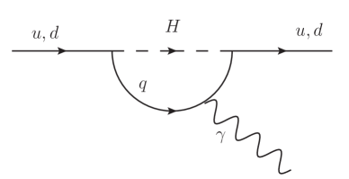
Figure 1: One loop diagrams for EDMs of $u$- and $d$-quarks with FC Higgs couplings. Here $q=s,b$ for an EDM of the $d$-quark and $q=c,t$ for an EDM of a $u$-quark.

III Diagrams with one FC coupling -and a $t\bar{t}H$-coupling

In Fig. 2 are shown some two loop diagrams for the EDM of a $d$-quark generated by exchange of one physical Higgs ($H$) boson and one $W$-boson, with a sizeable Higgs coupling $\sim g_{W}\,m_{t}/M_{W}$ to a top quark and where only one of the Higgs couplings are flavor changing (a soft photon is assumed to be added). The non-crossed version to the left in Fig. 2 does not give non-suppressed contributions. Taking crossed Higgs and $W$-bosons are equivalent to the topologies in the middle and right of Fig. 2.

Figure 2: Three diagrams with FC Higgs coupling for EDMs of a $d$-quark. Soft photon emission from one of the charged particles is assumed to be added. The left diagram will give contributions suppressed by $m_{u,d}/M_{W}$. Taking the crossed diagrams in the center or to the right, we will get contributions which are not suppressed by light quark masses. The diagram to the right is the complex conjugate of the diagram in the middle.

Adding a soft photon to the diagram in the middle and to the right, we get four diagrams for both cases. In Fig. 3 the four diagrams obtained by adding a soft photon emission to the diagram to the right in Fig. 2 are shown.

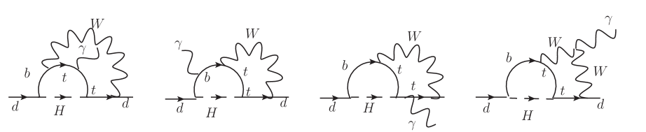
Figure 3: Four diagrams for an EDM of a $d$ quark obtained by adding a soft photon to the diagram to the right of Fig. 2. There are also corresponding diagrams where the $W$-boson is replaced by an unphysical Higgs-boson within Feynman gauge.

I have found that the results for the loop contributions in Fig. 3 have the form:

$${\cal M}(f\rightarrow f\gamma)_{(a)}\;=\;A\,\left(\bar{f}\,\sigma\cdot F\,P_{R}\,f\right)\,\,,$$ (10)

and that the diagrams with interchanged order of $H$ and $W$ loops, as in the middle of Fig. 2 have the form:

$${\cal M}(f\rightarrow f\gamma)_{(c)}\;=\;A^{*}\,\left(\bar{f}\,\sigma\cdot F\,P_{L}\,f\right)\,,$$ (11)

where $P_{L}=(1-\gamma_{5})/2$ and $P_{R}=(1+\gamma_{5})/2$ are projectors in Dirac space. Thus the electric dipole moment is found to be:

$$(d_{f})_{2-loop}=2\,Im(A)\;.$$ (12)

There is also a contribution to the magnetic moment (i.e the gyromagnetic quantity $(g-2)$) given by $2\,Re(A)$.

The contributions from the four diagrams ($i=$ 1-4) in Fig. 3 and its complex conjugates can then, by using (12) be written

$$(\frac{d_{d}}{e})_{i}\,=\hat{e}_{i}\,F_{2}\,S_{i}\,Im[Y_{R}(d\rightarrow b)\,V_{td}^{*}\,V_{tb}]\;,$$ (13)

where the $\hat{e}_{i}$’s are the electric charges (in units $e$= the proton charge) of the photon-emitting particles, i.e. $\hat{e}_{1,3}=\hat{e}_{t}=+2/3$, $\hat{e}_{2}=\hat{e}_{b}=-1/3$, and $\hat{e}_{4}=\hat{e}_{W}=+1$. Here I have used the relations (8) and (12). Note that a left-handed coupling $Y_{L}(d\rightarrow b)\,P_{L}$ would not contribute in (13) due to wrong chirality. The $V$’s are CKM matrix elements in the standard notation. The constant $F_{2}$ sets the overall scale of the EDMs obtained from the two loop diagrams:

$$F_{2}\,=\,\frac{g_{W}^{3}}{M_{W}\,\sqrt{2}}\left(\frac{1}{16\pi^{2}}\right)^{2}\,=\,\frac{2M_{W}^{2}}{v^{3}}\left(\frac{1}{16\pi^{2}}\right)^{2}\,\simeq\,6.94\times 10^{-22}\,\mbox{cm}\;,$$ (14)

where I have used the conversion rule $1/(200MeV)=10^{-13}$cm. The quantities $S_{i}$ in (13) are dimensionless functions of the masses of the particles entering the two loop diagrams. Some details from the loop calculations are given in the Appendix.

Using Feynman gauge for the $W$-boson, one has also to add diagrams with the unphysical Higgs field $\phi_{\pm}$ (i.e. the longitudinal component of the $W$-boson) given by the the Lagrangian

$${\cal L}_{\mathrm{\phi td}}\,=\,\;-\frac{g_{W}}{M_{W}}\,V_{td}^{*}\bar{d}\,\phi_{-}(m_{d}P_{L}\,-\,m_{t}P_{R})t\,+\,h.c.\;.$$ (15)

For finite loop diagrams, a typical example is given in (51)-(53), while other finite integrals are given with same type formulae with permuted masses, The loop functions $S_{1}$ and $S_{2}$ are finite, dimensionless, and depend on the mass ratios

$$u_{t}=(m_{t}/M_{W})^{2}=4.64\;\;,\quad u_{H}=(M_{H}/M_{W})^{2}=2.44\;.$$ (16)

The masses of the $W$-boson, the $t$-quark and the physical Higgs-boson $H$ are of the same order of magnitude. Therefore, because of lack of a clear mass hierarchy, it makes no sense to consider leading logarithmic approximations, in contrast to Fajer:2014ara . Numerically, I find

$$S_{1}=\,-\,2.55\;\;\;;\;\;S_{2}=2.50\;\,.$$ (17)

If the soft photon is emitted from the top quark after exchange of the Higgs boson, as in the third diagram from left in Fig. 3, or from the $W$-boson in the fourth diagram, the left sub-loop containing the Higgs boson is logarithmically divergent, which is not unexpected because the interaction in (9) is non-renormalizable. Each of the divergent integrals $\sim ln(\Lambda^{2})$ are followed by finite logarithmic terms more cumbersome than for finite loop integrals, and such integrals are given by expressions like in (58), also with masses permuted for different diagrams.

The total contribution from the third digram in Fig. 3, including the contribution from the unphysical Higgs, is

$$S_{3}\,=\,u_{t}\,p_{1}(u_{t})\,C_{\Lambda}+1.81\;.$$ (18)

Here the UV divergence is parametrized through the quantity

$$C_{\Lambda}\;\equiv\;ln(\frac{\Lambda^{2}}{M_{W}^{2}})\,+\,\frac{1}{2}\;\,,$$ (19)

where $\Lambda$ is the UV cut-off. Numerically, $C_{\Lambda}$ is $\sim 5.5$ to 9.4 for $\Lambda\sim$ 1 to 7 TeV. Furthermore, $u_{t}\,p_{1}(u_{t})$ is the result of the second subloop. Here

$$p_{1}(u)\,\equiv\,\frac{u}{(u-1)}\left(1-\frac{ln(u)}{u-1}\right)\;\;;\quad p_{1}(u_{t})=0.737\;,$$ (20)

where $u_{t}$ is given in (16).

The fourth diagram in Fig. 3 with the soft photon emitted from the $W$-boson again contains a divergent part, and the total contribution to the fourth diagram is

$$S_{4}\,=\,-\frac{3}{4}\,p_{2}(u_{t})\,C_{\Lambda}+2.98\;,$$ (21)

where

$$p_{2}(u)\,\equiv\,\frac{u}{(u-1)}\left(\frac{u\cdot ln(u)}{u-1}\,-1\right)\;\;;\quad p_{2}(u_{t})\,=\,1.219\;.$$ (22)

Summing all contributions from diagrams in Fig. 3, I find

$$(\frac{d_{d}}{e})_{Fig.3}\,=\,(1.65\,+\,1.37\,C_{\Lambda})\cdot F_{2}\;\cdot Im[Y_{R}(d\rightarrow b)\,V_{td}^{*}\,V_{tb}]\;.$$ (23)

There are in addition contributions from the same diagrams in Fig. 3, but with other quarks in the loop. If the $b$-quark is replaced by an $s$-quark, the CKM factors are two orders of magnitude smaller, and in addition $Y_{R}(d\rightarrow s)$ has a stricter bound from $K-\bar{K}$-mixing. If the $t$-quark is replaced by the $u$- or $c$-quark, the contributions are suppressed by $(m_{u}/m_{t})^{2}$ and $(m_{c}/m_{t})^{2}$, respectively.

There are also similar diagrams for EDM of an $u$-quark, i.e. like in Fig. 3 with the $t$- and the $b$-quarks interchanged. This amplitude has the same structure as in (13), and is proportional to the combination $Im[Y_{R}(u\rightarrow t)\cdot V_{tb}^{*}\,V_{ub}]$. But the $u$-quark EDM contributions will be neglected. First, the ordinary SM coupling of the Higgs will be proportional to $m_{b}/M_{W}$ instead of $m_{t}/M_{W}$ for the $d$-quark case. Then it turns out that the prefactors $S_{i}$ for $u$-quark EDM contributions are suppressed by a factor of order $(m_{b}/m_{t})^{2}\sim 10^{-3}$ compared to the analogous $d$-quark contributions. Second, even if the ratio between $Y_{R}(u\rightarrow t)$ and $Y_{R}(d\rightarrow b)$ would be of order $m_{t}/m_{b}$, the $u$-quark EDM contribution to the nEDM in (4) would still be suppressed by $|(\rho_{u}\cdot m_{b})/(\rho_{d}\cdot m_{t})|\,\sim 10^{-2}$ compared to the $d$-quark EDM contribution to the nEDM.

IV Diagrams with one FC coupling -and a $WWH$-coupling

We will now consider another class of two loop diagrams generated by FC Higgs-boson couplings. These diagrams shown in Fig. 4 have a big $WWH$-coupling $\sim g_{W}\,M_{W}$ and only one FC Higgs coupling to a fermion. These two loop diagrams are divided in three types: the (a)-diagrams with Higgs exchange to the left, the (b)-diagrams with Higgs exchange in the middle, and the (c)-diagrams with Higgs exchange to the right. In the limit of small external light quark momenta, which we work, the (b)-diagrams are zero due to (odd) momentum integration, or they are suppressed by small external quark masses. The (c)-diagrams are complex conjugates of the (a)-diagrams. Soft photon emission from one of the charged particles should of course be added in Fig. 4, as seen in Fig. 5 for the (a)-diagrams. The (a) diagrams give contributions like in (10), and the (c) diagrams like in (11).

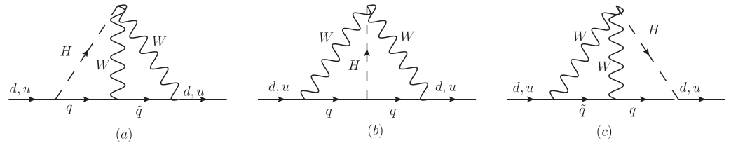
Figure 4: Three diagrams with one $WWH$-Higgs coupling and one FC Higgs coupling for EDMs of a $u$- or $d$-quark. Soft photon emission from one of the charged particles is assumed to be added. The (b) diagrams are zero in the limit of zero external momentum of the light quarks due to momentum integration, or are suppressed by small light quark masses. The (c) diagrams are complex conjugates of the (a) diagrams . Here $q=s,b$ and $\tilde{q}=u,c,t$ for EDM of a $d$-quark, and $q=c,t$ and $\tilde{q}=d,s,b$ for EDM of a $u$-quark.

The relevant piece of the SM Lagrangian for a Higgs coupling to two $W$-bosons is given by

$${\cal L}_{\mathrm{WWH}}\,=\,g_{W}\,M_{W}\,\sqrt{2}\,H\,W^{(-)\,\mu}\,W_{\mu}^{(+)}\;.$$ (24)

Using Feynman gauge for the $W$-boson, we must also consider Lagrangian terms for a physical Higgs coupling to a $W$-boson and the unphysical Higgs boson $\phi_{\pm}$. In addition to the term for quarks coupling to $\phi_{\pm}$ in (15), there is the relevant $HW\phi_{\pm}$- coupling obtained from the Lagrangian

$${\cal L}_{\mathrm{HW\phi}}\,=\,\frac{g_{W}}{\sqrt{2}}\left\{\,H\,(i\partial^{\mu}\phi_{-})\,-\,(i\partial^{\mu}\,H)\phi_{-}\right\}\,W_{\mu}^{(+)}\,+\,h.c.$$ (25)

Because of derivative couplings, the vertices involving the unphysical Higgs $\phi_{\pm}$ will depend on the loop momenta, which might give divergent (sub-)loops. There are also $W\gamma\phi_{\pm}$-couplings, but they do not contribute for soft photon emission.

In the preceeding section (III), for all the shown diagrams in Fig.3, the physical Higgs coupled to the top quark with strength $\sim g_{W}m_{t}/M_{W}$. Also the chiral structure of the diagrams is such that these diagrams are proportional to $m_{t}^{2}$, and even $m_{t}^{4}$ in $S_{3}$. In the present section the diagrams have a flavor blind $WWH$ coupling, and have another chiral structure, and one gets diagrams $\sim\,m_{t}^{2}$ only for the case when the $W$-boson is replaced by an unphysical Higgs $\phi_{\pm}$. Therefore I have apriori considered all quark flavors in the loops, although it is expected that the GIM-mechanism will cancel the leading terms with light quark flavors, except for the difference between the $t$-quark and the $c$-quarks contribution.

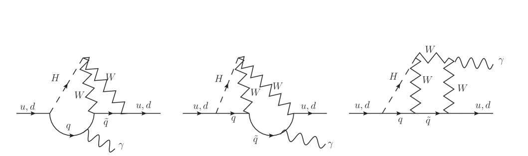
Figure 5: Emission of a soft photon from (a)-type diagrams of Fig. 4. There is also a diagram with emission from the $W$ in center of the diagram, and in addition graphs with the W replaced by an unphysical Higgs within Feynman gauge.

Contributions to the $d$-quark EDM from soft photon emission from the quark $q=s,b$ in the diagram 5a,( i.e. to the left in Fig. 5) can in the general case be written :

$$(\frac{d_{d}}{e})_{5a}\,=\,-\,2\,\hat{e}_{s}\,F_{2}\,\left\{\mbox{Im}\left[Y_{R}(d\rightarrow s)\,\lambda_{u}\right]\cdot\Delta f_{d}(s,u-c)+\mbox{Im}\left[Y_{R}(d\rightarrow s)\lambda_{t}\right]\cdot\Delta f_{d}(s,t-c)\right\}$$

$$-\,2\,\hat{e}_{b}\,F_{2}\,\left\{\mbox{Im}\left[Y_{R}(d\rightarrow b)\,\xi_{u}\right]\cdot\Delta f_{d}(b,u-c)+\mbox{Im}\left[Y_{R}(d\rightarrow b)\,\xi_{t}\right]\cdot\Delta f_{d}(b,t-c)\,\right\}\,,$$ (26)

where $F_{2}$ is given in (14) and where $\hat{e}_{s}=\hat{e}_{b}=-1/3$ are charges for the photon-emitting quarks, and the $\lambda$’s and the $\xi$’s are CKM factors:

$$\lambda_{\tilde{q}}=V_{\tilde{q}d}^{*}V_{\tilde{q}s}\;,\qquad\xi_{\tilde{q}}=V_{\tilde{q}d}^{*}V_{\tilde{q}b}\;,\qquad\tilde{q}=u,c,t\;\,.$$ (27)

The $\Delta f$’s in (29) are differences, due to GIM-cancellation, between loop functions $f(q,\tilde{q})$, for given flavors $q=s,b$ and $\tilde{q}=u,c,t$. These are functions of quark, $W$-boson and Higgs masses. Above, I have used the shortages

$$\Delta f_{d}(b,t-c)\;\equiv\;f(b,t)\,-\,f(b,c)\quad\;;\;\;\Delta f_{d}(s,c-u)\;\equiv\;f(s,c)\,-\,f(s,u)\;\,,$$ (28)

and so on in a self-explanatory way.

The quantities $f(q,\tilde{q})$ are finite, and are of order $10^{-1}$ to $1$. The GIM-cancellations for the difference between the $u$- and $c$-quark contributions are very efficient, such that the differences $\Delta f_{d}(s,u-c)$ and $\Delta f_{d}(b,u-c)$ are of order $10^{-3}$ to $10^{-7}$, and can be safely neglected. Contributions with the $t$-quark in the loops are significantly different from contributions involving the lighter quarks. Thus, the determination of both the $t$-quark and the $c$-quark contributions will be important. In this case the GIM cancellation is not efficient.

Contributions to the $d$-quark EDM from soft photon emission from the quark $q=s,b$ in the diagram 5a,the dominating contribution can be written :

$$(\frac{d_{d}}{e})_{5a}\,=\,-\,2\,\hat{e}_{b}\,F_{2}\,\left\{\mbox{Im}\left[Y_{R}(d\rightarrow b)\,\xi_{t}\right]\cdot\Delta f_{d}(b,t-c)\,\right\}\,,$$ (29)

where $F_{2}$ is given in (14) and where $\hat{e}_{b}=-1/3$ is the charge for the photon-emitting $b$-quark, and $\xi_{\tilde{q}}=V_{td}^{*}V_{tb}$. There are also other contributions which are small and can be neglected.

The quantity $\Delta f_{d}(b,t-c)$ from loop calculations is the difference between the $b\rightarrow t$ and the $b\rightarrow c$ contributions, and is given by

$$\Delta f_{d}(b,t-c)\simeq-0.34\;.$$ (30)

The diagram with soft photon emission from the quark $\tilde{q}=u,c,t$, is shown the center of Fig. 5 (i.e Fig. 5b). Adding contributions where the $W$ is replaced by an unphysical Higgs $\phi_{\pm}$, one obtains divergent contributions for these loop functions.

Because the $WH\phi_{\pm}$-vertex is momemtum dependent, the left subloop is divergent, reflecting again that the theory based on the Lagrangian in eq. (7) alone is not renormalizable. The numerically relevant term from diagram 5b is given by

$$(\frac{d_{d}}{e})_{5b}\,\simeq\,+2\,\hat{e}_{\tilde{q}}\,F_{2}\cdot\mbox{Im}\left[\xi_{t}\,Y_{R}(d\rightarrow b)\right]\cdot\Delta h_{d}(b,t-c)\;\,,$$ (31)

where $\Delta h_{d}(b,t-c)$ is defined similar to the $\Delta f$’s in eq.(28). In this case there is a divergent term when $W$ is replaced by the unphysical Higgs $\phi_{\pm}$, and the total result from diagram 5b is

$$\Delta h_{d}(b,t-c)\,=\,p_{2}(u_{t})\,C_{\Lambda}-1.26\;,$$ (32)

where $C_{\Lambda}$ is given in (19) and $p_{2}(u)$ in (22).

An example for diagrams with a soft photon emitted from the $W$-boson is shown at the right of Fig. 5 (Fig. 5c). Also in this case there are divergent diagrams, because the left sub-loop might be divergent for the replacement $W\rightarrow\phi_{\pm}$. After GIM-cancellation the dominant term is

$$(\frac{d_{d}}{e})_{5c}\,\simeq\,3\,\hat{e}_{W}\,F\,\cdot\mbox{Im}\left[Y_{R}(d\rightarrow b)\,\xi_{t}\right]\cdot\Delta k_{d}(b,t-c)\,\,,$$ (33)

where one finds

$$\Delta k_{d}(b,t-c)\,=\,\frac{1}{2}p_{2}(u_{t})\,C_{\Lambda}-2.48$$ (34)

Neglecting small contributions (all except those proportional to $V_{td}^{*}\,V_{tb}\,\equiv\xi_{t}$), and summing all contributions from diagrams in Fig. 5 one finds

$$(\frac{d_{d}}{e})_{Fig.5}\,=\,(3.46\,C_{\Lambda}-9.35)\cdot F_{2}\cdot Im[Y_{R}(d\rightarrow b)\,V_{td}^{*}\,V_{tb}]$$ (35)

The EDM of the $u$-quark is neglected due to small loop functions (-after GIM-cancellation), small CKM-factors. Moreover, the comments about the $Y_{R}$’s at the end of the previous sections are also relevant here.

V Perturbative QCD corrections

Summing all two loop contributions from section III and IV, I obtain the total bare dominanting contribution for an EDM of the $d$-quark:

$$(\frac{d_{d}}{e})_{Tot}^{bare}\,=\,\equiv C_{E}(\mu_{\Lambda})(4.83\,=\,C_{\Lambda}-7.70)\,F_{2}\,\,Im[Y_{R}(d\rightarrow b)\,V_{td}^{*}\,V_{tb}]\;.$$ (36)

But perturbative QCD effects must also been taken into account. The color electric term can be easily found from the same expressions for photon emission from quarks (corresponding to all quark charges put to $+g_{s}$). The total color electric term is then found to be

$$(\frac{d_{d}}{g_{s}})_{Tot}^{bare}\,=\,C_{C}(\mu_{\Lambda})\,=\,(1.96\,C_{\Lambda}-2.55)\,F_{2}\,\,Im[Y_{R}(d\rightarrow b)\,V_{td}^{*}\,V_{tb}]\;.$$ (37)

There are also contributions from the Weinberg operator for the FCH couplings. Contributions to the Weinberg operator proportional to $Im[Y_{R}(d\rightarrow b)\,V_{td}^{*}\,V_{tb}]$, are shown in Fig. 6. These are however very small due to “wrong” chiralities, are suppressed by $m_{d}/M_{W}$, and will therefore be neglected.

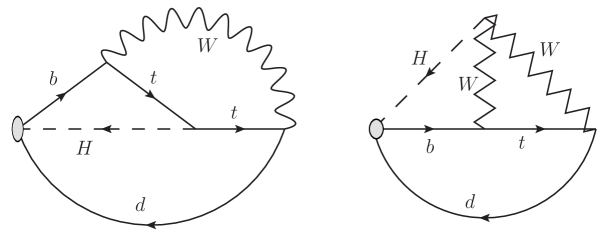
Figure 6: The contributions to the Weinberg operator for the flavor changing Higgs interaction $Y_{R}(d~{}\rightarrow~{}b)$, represented by the grey blobs to the left in both diagrams. Three gluon lines have to be attached to quark lines.

The color electric term mixes into the EDM term in (3) due to renormalization effects in perturbative QCD. The relevant mixing matrix under QCD renormalization at one loop level is given in Degrassi:2005zd . This result is also used in Gorbahn:2014sha . The result for the coefficient $C_{E}$ of the EDM-operator describing the running from a high scale $\mu_{high}$ down to a smaller scale $\mu_{low}$ is

$$C_{E}(\mu_{low})\,=\,\eta^{\kappa_{E}}C_{E}(\mu_{high})\,+\,\frac{\gamma_{CE}}{\gamma_{E}\,-\gamma_{C}}\,(\eta^{\kappa_{E}}\,-\,\eta^{\kappa_{C}})\,C_{C}(\mu_{high})\;.$$ (38)

There is also a term due to the Weinberg operator which is omitted here because of the negligible contribution mentioned above. In this one loop formula, $\gamma_{E}$ and $\gamma_{C}$ are the anomalous dimensions of the EDM- and the color electric operators, respectively, and $\gamma_{CE}$ describes the mixing of the color operator into the EDM operator. One has

$$\gamma_{E}\,=\,\gamma_{CE}\,=\frac{32}{3}\,\;,\;\gamma_{C}\,=\frac{28}{3}\,,$$ (39)

and

$$\kappa_{i}\,=\,\frac{\gamma_{i}}{2\beta_{0}}\;\,;\;\eta\,=\,\frac{\alpha_{s}(\mu_{high})}{\alpha_{s}(\mu_{low})}\;\,;\;\beta_{0}\,=\,11-\frac{2n_{f}}{3}\,,$$ (40)

where $n_{f}$ is the number of active quark flavors, which is $n_{f}=6$ above the $t$-quark scale and $n_{f}=5$ below. In the present case one should do the running in four steps, from the big scale $\mu_{\Lambda}\sim\Lambda$ down to the top scale $\mu_{t}\sim m_{t}$ with $\beta_{0}=7$, from the top scale down to the $b$-quark scale $m_{b}$ with $\beta_{0}=23/3$, brom the $b$-quark scale down to the charm scale $m_{c}$ with $\beta_{0}=25/3$, and at last from the charm scale down to the hadronic scale $\mu_{h}\sim$ 1 GeV with $\beta_{0}=9$.

Including QCD corrections, I obtain at the hadronic scale $\mu_{h}$ = 1 GeV:

$$d_{d}/e\,=\,C_{e}(\mu_{h})\,=\,K_{1}\,\eta^{\frac{16}{21}}\,C_{E}(\mu_{\Lambda})\,+\,\left(K_{1}\,(\eta^{\frac{16}{21}}-\eta^{\frac{14}{21}})\,+\,K_{5}\,\eta^{\frac{14}{21}}\right)\,C_{C}(\mu_{\Lambda})\;.$$ (41)

where $\eta\equiv\alpha_{s}(\mu_{\Lambda})/\alpha_{s}(\mu_{t})$, and where $K_{1}$ and $K_{5}$ takes care of the QCD corrections below $\mu_{t}$, and are given in eqs. (60) - (64) in the Appendix. The one loop result should be a good approximation above top mass scale, but not for lower scales, i.e. not below say, the $b$-quark scale.

VI SUMMARY and DISCUSSION

As expected, there are cases where the considered two loop diagrams for the EDMs of $d$- and $u$-quarks diverges. This happens for cases in section III where the left sub-loop in Fig. 7 is involved, and for diagrams where the unphysical Higgs ($\phi_{\pm}$) is involved both in sect III and IV. More specific, the left diagram in Fig. 7 which looks like a vertex correction for $d\rightarrow W\,+\,u,c,t$ is logarithmically divergent. Actually, this diagram generates a logarithmic divergent right-handed current which has no match in the SM. The diagram at the right in Fig. 7 is convergent, but if the $W$-boson is replaced by an unphysical Higgs $\phi_{\pm}$, when used in two loop diagrams as in Fig. 5, we obtain logarithmic divergent diagrams due to a momentum dependent vertex, as seen from (25). These are numerically relevant if the quark $\tilde{q}$ is a top quark. The dominating divergent terms in section III and IV are proportional to $m_{t}^{2}$ (-or even $m_{t}^{4}$ in one case in section III). It should also be noted that the first and last diagram in Fig. 5 are relevant for the EDM of the electron Altmannshofer:2015qra . However, in that case the divergent terms would be proportional to powers of a tiny neutrino mass, instead of the top-quark mass.

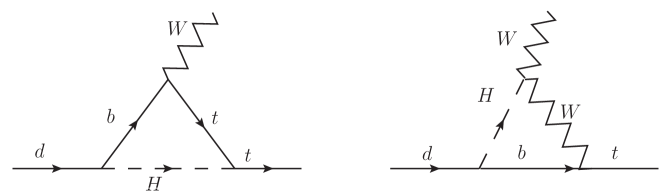
Figure 7: The divergent effective W-loop vertex correction diagram relevant for diagrams of section III (left), and the (finite) effective vertex correction relevant for diagrams in section IV (right).

All contributions (after GIM-cancellation) not proportional to $\xi_{t}\,\equiv\,V_{td}^{*}\,V_{tb}$ are neglected, using bounds on other $Y_{R}$’s Blankenburg:2012ex ; Harnik:2012pb , as explaned in the preceeding sections. Also all the contributions for an EDM of the $u$-quark can be neglected, for reasons given at the end of the sections III and IV.

I have also neglected the $s$-quark contribution $d_{s}$ for the following reason: The loop functions for the $s$-quark are numerically close to the ones for the $d$-quark. The CKM factor is bigger, but $\gamma_{s}/\gamma_{d}\simeq 10^{-2}$, such that the contribution to the result in (4) from the $d_{s}$ is of order $5\%$. Thus our final result for the nEDM is simply

$$d_{n}\;\simeq\;\rho_{d}\,d_{d}\;,$$ (42)

where the lattice value of $\rho_{d}$ is given in (6). Using the experimental bound for nEDM in (1), the result (36) of the present study gives the bound

$$|\mbox{Im}\left[Y_{R}(d\rightarrow b)\cdot\frac{V_{td}^{*}\,V_{tb}}{|V_{td}^{*}\,V_{tb}|}\right]|\leq(1.2\;\,\mbox{to}\;\,2.2)\times 10^{-3}\;.$$ (43)

for values of $\Lambda$ from one up to seven TeV.

From the mathematical point of view, $\Lambda$ is the quantity which regularise the divergent two loop diagrams, while $\Lambda_{NP}$ in (9) is introduced as a dimensional quantity parametrising the $Y_{R}$’s and indicates the scale of new physics. But these scales are expected to be of the same order of magnitude.

In (43) I have found a bound on the imaginary part of the coupling $Y_{R}(d\rightarrow b)$ multiplied by the CKM entry $V_{td}^{*}V_{tb}$ (-remenbering that $V_{tb}\simeq 1$). Thus the present bound is not directly comparable to the previous bound $1.5\times 10^{-4}$ on the absolute value of $Y_{R}(d\rightarrow b)$ given in refs. Blankenburg:2012ex ; Harnik:2012pb . But, turning things around, if the bound for $Y_{R}(d\rightarrow b)$ found in Harnik:2012pb is assumed to be saturated, then one can see how close to the experimental bound on the nEDM in (1) my value of nEDM might come. This is illustrated explicitly as follows:

Using (36), the lattice values in (6) and absolute value of $V_{td}^{*}\,V_{tb}$ from Olive:2016xmw , one may write my result for the nEDM in the following way

$$d_{n}/e\simeq N(\Lambda)\times\left\{\frac{|Y_{R}(b\rightarrow d)|}{|Y_{R}(b\rightarrow d)|_{Bound}}\cdot\mbox{Im}\left[\frac{Y_{R}(d\rightarrow b)}{|Y_{R}(b\rightarrow d)|}\cdot\frac{V_{td}^{*}\,V_{tb}}{|V_{td}^{*}\,V_{tb}|}\right]\right\}\times 10^{-26}\,\mbox{cm}\;,$$ (44)

where I have scaled the result with the bound from Blankenburg:2012ex ; Harnik:2012pb :

$$|Y_{R}(d\rightarrow b)|\;\leq\;1.5\times 10^{-4}\;\equiv\;|Y_{R}(d\rightarrow b)|_{Bound}\,.$$ (45)

Defining first

$$C_{a}\,=\,F_{2}\,Im[Y_{R}(d\rightarrow b)\,V_{td}^{*}\,V_{tb}]\,\hat{C}_{a}\,,$$ (46)

for $a=E,C$, I further define the function $N(\Lambda)$, by the relation

$$\rho_{d}\,F_{2}\,|Y_{R}(d\rightarrow b)|_{Bound}|V_{td}^{*}\,V_{tb}|\,\hat{C_{E}}(\mu_{\Lambda})=\,N(\Lambda)\,\times 10^{-26}\,\mbox{cm}\,.$$ (47)

The function $N(\Lambda)$ is plotted as a function of $\Lambda$ in Fig. 8.

Now, the maximal value of the parenthesis $\{...\}$ in (44) is $=1$. Then, if the bound for $Y_{R}(d\rightarrow b)$ is saturated, the plot for the function $N_{\Lambda}$ in Fig. 8 shows that when the cut-off $\Lambda$ is stretched up to 20 TeV, the bound for nEDM in (1) is reached in the bare case, while the perturbative QCD-suppression tells us that the value of the nEDM can at maximum be of order one tenth of the experimental bound for $\Lambda$ up to 20 TeV. If the bound for $|Y_{R}(d\rightarrow b)|$ is reduced, and also $\Lambda$ is reduced, my value for nEDM will be accordingly smaller.

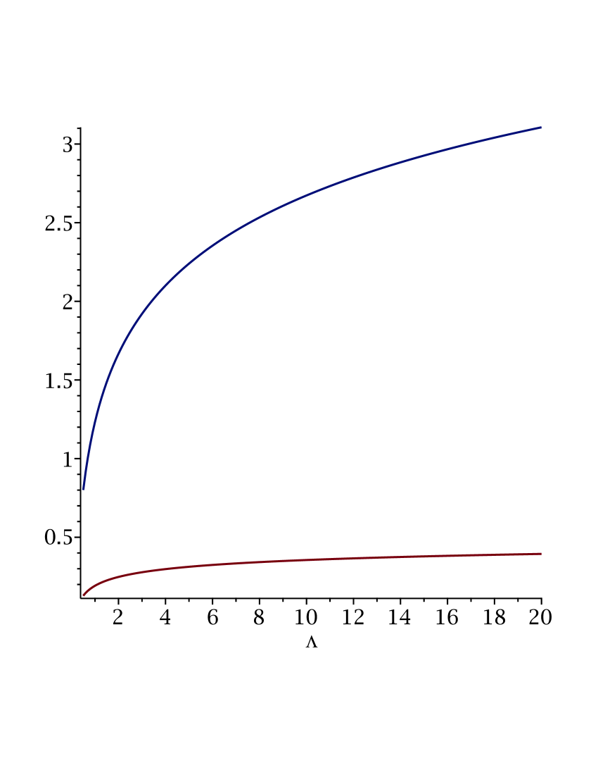
Figure 8: The quantity $N(\Lambda)$, in units $10^{-26}$ cm, as a function of cut-off $\Lambda$ (in TeV)

VII Conclusion

In conclusion, I have explored the consequenses for the nEDM of having flavor changing Higgs couplings. In the scenary of Harnik:2012pb ; Dorsner:2015mja such couplings might stem from a six dimensional non-renormalizable, $SU(2)_{L}\times U(1)_{Y}$ gauge-invariant Lagrangian piece proportional to the third power of the SM Higgs doublet field, as seen in eq. (9). While previous analysis Blankenburg:2012ex ; Harnik:2012pb obtained bound(s) of quadratic expressions of the FCH coupling(s), in the present paper the analysis is extended to the two loop case for quark EDMs generated by a flavor changing Higgs coupling $Y_{R}(d\rightarrow d)$ to first order only.

I have found and calculated two loop contributions which gives a bound for the imaginary part of the product of $Y_{R}(d\rightarrow b)$ and the CKM entry $V_{td}^{*}V_{tb}$ (where $V_{tb}$ is known to be very close to one). This bound cannot be directly compared with the bound from Blankenburg:2012ex ; Harnik:2012pb , which is on the absolute value. But even if this bound on the absolute value is saturated, and even if $\Lambda$ is stretched up to 20 TeV, it is seen from Fig. 8 that the value of the nEDM can at maximum be of order one tenth of the present experimental bound in (1).

VIII Appendix

Many loop diagrams are suppressed because of chirality ($P_{L}\,P_{R}\,=\,0$), or asymmetric (odd) momentum integration like:

$$\int d\hskip-3.99994pt^{-}\,p\,f(p^{2};\mbox{masses})\,p^{\mu}\,=\,0\;\,.$$ (48)

To simplify calculations I use the effective quark propagator in a soft electromagnetic field $F$ Reinders:1984sr :

$$S_{1}(k,F)\;=\;(-\frac{e_{q}}{4})\;\frac{\left\{(\gamma\cdot k+m_{q})\,,\,\sigma\cdot F\right\}}{(k^{2}-m_{q}^{2})^{2}}\;\;,$$ (49)

where $k$ is the four momentum and $m_{q}$ the mass of the quark $q$. The notation $\{A,B\}\equiv AB+BA$ is used. Similarly, for emission of a soft photon from a $W$-boson, the effective propagator is:

$$(D_{1}(k,F))^{\alpha\beta}\;=\;(-\frac{e_{W}}{4})\;\frac{3\,i\,\left(g^{\mu\alpha}g^{\nu\beta}-g^{\mu\beta}g^{\nu\alpha}\right)\,F_{\mu\nu}}{(k^{2}-M_{W}^{2})^{2}}\;\,.$$ (50)

These effective propagators can be used and are useful when the particles in the loop are much bigger that the masses of the external particles.

A typical example for a finite loop integral is

$$T_{\mu\nu}\,=\,\int\frac{d\hskip-3.99994pt^{-}p\,d\hskip-3.99994pt^{-}r\;p_{\mu}\,r_{\nu}}{(p^{2}-M_{H}^{2})(p^{2}-m_{b}^{2})((r-p)^{2}-M_{W}^{2})(r^{2}-M_{W}^{2})(r^{2}-m_{t}^{2})^{2}}.\,\;$$ (51)

where $d\hskip-3.99994pt^{-}r\equiv d^{4}r/(2\pi)^{4}$. Integrating out momenta, the result of the loop integration gives:

$$T_{\mu\nu}\,=\,\left(\frac{1}{16\pi^{2}}\right)^{2}\,\frac{g_{\mu\nu}}{4M_{W}^{2}}\,a(m_{t}^{2},M_{W}^{2},M_{H}^{2})\,,$$ (52)

where the dimensionless loop function $a(m_{t}^{2},\,M_{W}^{2},\,M_{H}^{2})$ can be written in the compact form

$$a(m_{t}^{2},\,M_{W}^{2},\,M_{H}^{2})\,=\,\int_{0}^{1}dx\,\int_{0}^{(1-x)}dy\,\frac{xyM_{W}^{2}}{x(1-x)(M_{F}^{2}-M_{H}^{2})}\left[\,1\,-\,\frac{M_{H}^{2}}{M_{F}^{2}-M_{H}^{2})}\,ln(\frac{M_{F}^{2}}{M_{H}^{2}})\right]$$ (53)

where the quantity $M_{F}^{2}$ depends on masses and Feynman parameters:

$$M_{F}^{2}\,=\,\frac{M_{W}^{2}\,+\,y(m_{t}^{2}\,-\,M_{W}^{2})}{x(1-x)}\;.$$ (54)

The expression in (53) can be further found in terms of logarithmic and dilogarithmic functions. Other finite terms are given with formulae as (51)-(53), but with masses permuted. A term with ultraviolet divergence appears if $r_{\nu}$ is replaced by $p_{\nu}$ in the numerator when doing loop integration in the subloop containing the integration over $p$. This happens for instance when the $W$-boson is replaced by an unphysical Higgs $\phi_{\pm}$ (the longitudinal $W$-components) within Feynman gauge, or if the left diagram in Fig. 7 is involved. In addition to $a(m_{t}^{2},\,M_{W}^{2},\,M_{H}^{2})$, the loop diagrams in section III wil be proportional to $m_{t}^{2}/M_{W}$.

Divergent parts from the first subloop enters as

$$ln(\Lambda^{2}/R)\;,$$ (55)

where $R=Q-x(1-x)r^{2}$, where $Q$ is a quantity depending on masses and Feynman paprameters.(for inst $Q=M_{W}^{2}x+M_{H}^{2}y$, where $x$ and $y$ are Feynman parameters of the first, divergent, subloop). The $ln(R)$ term results in a finite term . For example, for third diagram (with $W^{\pm}\rightarrow\phi_{\pm}$, one obtains :

$$S_{3N}^{\phi}\,=\,-\,\frac{u_{t}^{2}}{(u_{H}-b)}\,\int_{0}^{1}dx\,x(1-x)[N(1,u_{t};B_{1})-N(1,u_{t};B_{0})]\,=\,-1.90\;,$$ (56)

where $B_{0,1}$ are given as

$$B_{0}\,=\;\frac{b+x(u_{t}-b)}{x(1-x)}\;;\;B_{1}\,=\,\frac{u_{H}+x(u_{t}-u_{H})}{x(1-x)}\;,$$ (57)

where $u_{t}$ and $u_{H}$ are given in (16), and $b\equiv m_{b}^{2}/M_{W}^{2}$.

$$N(C,A;B)\,\equiv\,\frac{(A^{2}-AB)}{C-A}\left(\frac{ln(B)}{A}+\frac{ln(\frac{B}{A})}{(B-A)}\right)$$

$$+\,\frac{C(C-B)}{(C-A)^{2}}\{\frac{1}{2}[ln(B-C)]^{2}+dilog(\frac{B}{B-C})\,-\,ln(C)\cdot ln(B-C)\}\,$$

$$+\,\frac{[BC-A(2C-A)]}{(C-A)^{2}}\{\frac{1}{2}[ln(B-A)]^{2}+dilog(\frac{B}{B-A})\,-\,ln(A)\cdot ln(B-A)\}\,.$$ (58)

Further, there is a non-logarithimic finite term (not in $ln(R)$ in eq. (55)): For other divergent diagrams one has similar expressions with permuted masses.

The dilogarithmic function is in my case defined as

$$dilog(z)\,\equiv\,\int_{1}^{z}dt\frac{ln(t)}{(1-t)}\;=\,\int_{0}^{1}\frac{dx}{x}ln(1-(1-z)x)\,=\,Li_{2}(1-z)\,.$$ (59)

The QCD correction factors in (41) are

$$K_{1}\,=\,(\frac{\alpha_{s}(\mu_{c})}{\alpha_{s}(\mu_{h})})^{\frac{16}{27}}\,(\frac{\alpha_{s}(\mu_{b})}{\alpha_{s}(\mu_{c})})^{\frac{16}{25}}\,(\frac{\alpha_{s}(\mu_{t})}{\alpha_{s}(\mu_{b})})^{\frac{16}{23}}\;,$$ (60)

$$K_{2}\,=\,8\left((\frac{\alpha_{s}(\mu_{c})}{\alpha_{s}(\mu_{H})})^{\frac{16}{27}}\,(\frac{\alpha_{s}(\mu_{b})}{\alpha_{s}(\mu_{c})})^{\frac{16}{25}}\,[(\frac{\alpha_{s}(\mu_{t})}{\alpha_{s}(\mu_{b})})^{\frac{16}{23}}\,-\,(\frac{\alpha_{s}(\mu_{t})}{\alpha_{s}(\mu_{b})})^{\frac{14}{23}}]\right)\;,$$ (61)

$$K_{3}\,=\,8\left((\frac{\alpha_{s}(\mu_{c})}{\alpha_{s}(\mu_{h})})^{\frac{16}{27}}\,[(\frac{\alpha_{s}(\mu_{b})}{\alpha_{s}(\mu_{c})})^{\frac{16}{25}}\,-\,(\frac{\alpha_{s}(\mu_{b})}{\alpha_{s}(\mu_{c})})^{\frac{14}{25}}]\,(\frac{\alpha_{s}(\mu_{t})}{\alpha_{s}(\mu_{b})})^{\frac{16}{23}}\right)\;,$$ (62)

$$K_{4}\,=\,8\left([(\frac{\alpha_{s}(\mu_{c})}{\alpha_{s}(\mu_{h})})^{\frac{16}{27}}\,-\,(\frac{\alpha_{s}(\mu_{c})}{\alpha_{s}(\mu_{H})})^{\frac{14}{27}}]\,(\frac{\alpha_{s}(\mu_{b})}{\alpha_{s}(\mu_{c})})^{\frac{16}{25}}\,(\frac{\alpha_{s}(\mu_{t})}{\alpha_{s}(\mu_{b})})^{\frac{16}{23}}\right)\;,$$ (63)

and

$$K_{5}\,=\,K_{2}\,+\,K_{3}\,+\,K_{4}\;.$$ (64)

One could consequently stick to one-loop values for $\alpha_{s}(\mu)$ at the various scales. However, I have used a hybrid version, taking into acount higher loop effects (see for example Deur:2016tte ) which are important below $\mu_{b}=m_{b}$, say. Then I have used $\alpha_{s}(\mu_{t})=0.109$, $\alpha_{s}(\mu_{b})=0.23$, $\alpha_{s}(\mu_{c})=0.40$, and $\alpha_{s}(\mu_{h})=0.52$.

- [1] M. Pospelov and A. Ritz, Annals Phys. 318 (2005) 119 [hep-ph/0504231]
- [2] T. Fukuyama, Int. J. Mod. Phys. A27 (2012) 1230015, arXiv: 1201.4252 [hep-ph]
- [3] W. Dekens, J. de Vries, J. Bsaisou, W. Bernreuther, C. Hanhart, Ulf-G. Meißner, A. Nogga, and A. Wirzba JHEP 07 (2014) 069, arXiv:1404.6082[hep-ph]
- [4] M. Jung and A. Pich, JHEP 1404 076, arXiv:1308.6283 [hep-ph]
- [5] N. Yamanaka, B.K. Sahoo, N. Yoshinaga, T. Sato, K. Asahi, and B. P Das, Eur. Phys. J., A53 (2017) 54, arXiv: 1703.01570 [hep-ph]
- [6] K. A. Olive et al [Particle Data Group Collaboration] : “Review of Particle Physics”, Chin. Phys. C40 (2016) 100001
- [7] C. A. Baker, D. D. Doyle, P. Geltenbort, K. Green, M. G. D. van der Grinten, P. G. Harris, P. Iaydjiev and S. N. Ivanov et al., Phys. Rev. Lett. 97 (2006) 131801 [hep-ex/0602020].
- [8] E.P. Shabalin, E.P., Yad.Fiz. 31 (1980)1665-1679 (Sov. J. Nucl.Phys. 31 (1980) 864)
- [9] A. Czarnecki, and B. Krause, Phys.Rev.Lett. 78 (1997) 4339 [hep-ph/97043559]
- [10] A. Maiezza, and M. Nemevšek, Phys. Rev. D 90 (2014) 095002, arXiv:1407.3678 [hep-ph]
- [11] D.V. Nanopoulos, A. Yildiz, and P. H. Cox, Phys.Lett. B87 53
- [12] B.F. Morel, Nucl.Phys. B157 (1979) 23
- [13] M.B. Gavela, A. Le Yaouanc, L. Oliver,O. Pene J.C. Raynal, and T.N. Pham, Phys.Lett. B109 (1982) 215
- [14] I.B. Khriplovich and A.R. Zhitnitsky, Phys.Lett. B109 (1982) 490
- [15] B.H.J. McKellar,S.R. Choudhury, X.-G. He and S. Pakvasa, Phys.Lett. B197 (1987) 556
- [16] J.O. Eeg, J.O. and I. Picek, Phys.Lett. B130 (1983) 308
- [17] J.O. Eeg, and I. Picek, Nucl.Phys. B244 (1984) 77
- [18] C. Hamzaoui and A. Barroso, Phys. Lett. B 154, 202 (1985).
- [19] T. Mannel and N. Uraltsev, Phys. Rev. D 85 (2012) 096002, arXiv:1202.6270 [hep-ph]
- [20] T. Bhattacharya, V. Cirigliano, R. Gupta, H-W. Lin, and B. Yoon, Phys. Rev. Lett. 115 (2015) 212002, arXiv:1506.04196 [hep-lat]
- [21] T. Bhattacharya, V. Cirigliano, S. D. Cohen, R. Gupta, A. Joseph, H-W. Lin, and B. Yoon, Phys. Rev. D 92 (2015)094511 , arXiv:1506.06411 [hep-lat]
- [22] W. Buchmuller and D. Wyler, Phys.Lett. B121 (1983) 321
- [23] W. Altmannshofer, A. J. Buras and P. Paradisi, Phys. Lett. B 688 (2010) 202 [arXiv:1001.3835 [hep-ph]].
- [24] A. J. Buras, G. Isidori and P. Paradisi, Phys. Lett. B 694 (2011) 402, arXiv:1007.5291 [hep-ph]
- [25] J. Brod, U. Haisch, and J. Zupan, JHEP 1311 (2013) 180, arXiv:1310.1385 [hep-ph]
- [26] A. V. Manohar and M. B. Wise, Phys. Rev. D 74 (2006) 035009 [hep-ph/0606172].
- [27] G. Degrassi and P. Slavich, Phys. Rev. D 81 (2010) 075001, arXiv:1002.1071 [hep-ph]
- [28] Xiao-Gang He, Chao-Jung Lee, Siao-Fong Li, and J. Tandean, arXiv:1404.4436 [hep-ph]
- [29] J. M. Arnold, B. Fornal and M. B. Wise, Phys. Rev. D 87 (2013) 075004, arXiv:1212.4556 [hep-ph]
- [30] K. Fuyuto, J. Hisano, and E. Senaha, arXiv:1510.04485 [hep-ph]
- [31] L. Bian, and N. Chen, arXiv: 1608.07975 [hep-ph]
- [32] S. Fajfer, and J.O. Eeg, Phys. Rev. D89 (2014) 095030, arXiv:1401.2275 [hep-ph]
- [33] W. Altmannshofer, R. Primulando, C. -T. Yu and F. Yu, JHEP 1204 (2012) 049, arXiv:1202.2866 [hep-ph]
- [34] A. Goudelis, O. Lebedev, and J-h. Park, Phys. Lett. B707 (2012) 369-374, arXiv:1111.1715 [hep-ph]
- [35] G. Blankenburg, J. Ellis, and G. Isidori, Phys. Lett. B712 (2012) 386-390; arXiv:1202.5704 [hep-ph]
- [36] R. Harnik, J. Kopp and J. Zupan JHEP 03 (2013) 036, arXiv:1209.1397 [hep-ph]
- [37] A. Greljo, and J.F. Kamenik, and J. Kopp, JHEP 07 (2014) 046 arXiv 1404.1278 [hep-ph]
- [38] M. Gorbahn, and U. Haisch, JHEP 06 (2014) 033, arXiv 1404.4873 [hep-ph]
- [39] I. Doršner, S. Fajfer, A. Greljo, J. Kamenik, N. Košnik, and I. Nišandžic, JHEP 06 (2015) 108, arXiv 1502.07784 [hep-ph]
- [40] S.M. Barr and A. Zee, Phys. Rev. Lett. 65 (1990) 21-24 [Erratum: Phys. Rev. Lett. 65 (1990) 2920]
- [41] D.Chang, W.S. Hou, and W.-Y. Keung,, Phys. Rev.D48 (1993) 217; hep-ph/9302267
- [42] R.G. Leigh, R. G., S. Paban, S. and R. M. Xu, Nucl. Phys. B352 (1991) 45-58
- [43] J.D. Bjorken, and S. Weinberg, Phys. Rev. Lett. 38 (1977) 622
- [44] G.F. Giudice, and O. Lebedev, Phys. Lett. B665 (2008) 79-85, arXiv: 0804.1753 [hep-ph]
- [45] W. Altmannshofer, J. Brod, and M. Schmaltz, JHEP 05 (2015) 125, arXiv: 1503.04830 [hep-ph]
- [46] G. Degrassi, E. Franco, S. Marchetti, and L. Silvestrini,, JHEP, 11 (2005) 044 arXiv: 0510137 [hep/ph]
- [47] L.J Reinders, H. Rubinstein, and S. Yazaki, Phys.Rept. 127 (1985) 1
- [48] A. Deur, S.J. Brodsky, and G. F de Teramond, Prog. Part. Nucl. Phys. 90 (2016) 1-74. arXiv: 1604.08082 [hep-ph].