Robust regression for mixed Poisson-Gaussian model

Abstract

This paper focuses on efficient computational approaches to compute approximate solutions of a linear inverse problem that is contaminated with mixed Poisson–Gaussian noise, and when there are additional outliers in the measured data. The Poisson–Gaussian noise leads to a weighted minimization problem, with solution-dependent weights. To address outliers, the standard least squares fit-to-data metric is replaced by the Talwar robust regression function. Convexity, regularization parameter selection schemes, and incorporation of non-negative constraints are investigated. A projected Newton algorithm is used to solve the resulting constrained optimization problem, and a preconditioner is proposed to accelerate conjugate gradient Hessian solves. Numerical experiments on problems from image deblurring illustrate the effectiveness of the methods.

Keywords

Poisson-Gaussian model, weighted least squares, robust regression, preconditioner, image restoration

AMS classification

65N20 49M15 62F35

1 Introduction

In this paper we consider efficient computational approaches to compute approximate solutions of a linear inverse problem,

$$b=Ax_{\text{true}}+\eta,\quad\quad A\in\mathbb{R}^{m\times n},$$ (1)

where $A$ is a known matrix, vector $b$ represents known acquired data, $\eta$ represents noise, and vector $x_{\text{true}}$ represents the unknown quantity that needs to be approximated. We are particularly interested in imaging applications where $x_{\text{true}}\geq 0$ and $Ax_{\text{true}}\geq 0$. Although this basic problem has been studied extensively (see, for example, [9, 15, 26, 32] and the references therein), the noise is typically assumed to come from a single source (or to be represented by a single statistical distribution) and the data to contain no outliers. In this paper we focus on a practical situation that arises in many imaging applications, and for which relatively little work has been done, namely when the noise is comprised of a mixture of Poisson and Gaussian components and when there are outliers in the measured data. While some research has been done on the two topics separately (i.e., mixed Poisson–Gaussian noise models or outliers in measured data), to our knowledge no work has been done when the measured data contains both issues. In the following, we review some of the approaches used to handle each of the issues.

Poisson–Gaussian noise

A Poisson–Gaussian statistical model for the measured data takes the form

$$b_{i}=n_{\text{obj}}(i)+g(i),\ i=1,\ldots,m,\quad\ n_{\text{obj}}(i)\sim\text{Pois}([Ax_{\text{true}}]_{i}),\ g(i)\sim\mathcal{N}(0,\sigma^{2}),$$ (2)

where $b_{i}$ is the $i$th component of the vector $b$ and $[Ax_{\text{true}}]_{i}$ the $i$th component of the true noise-free data $Ax_{\text{true}}$. We assume that the two random variables $n_{\text{obj}}(i)$ and $g(i)$ are independent. This mixed noise model arises in many important applications, such as when using charged coupled device (CCD) arrays, x-ray detectors, and infrared photometers [2, 12, 21, 22, 30]. The Poisson part (sometimes referred to as shot noise) can arise from the accumulation of photons over a detector, and the Gaussian part usually is due to read-out noise from a detector, which can be generated by thermal fluctuations in interconnected electronics.

Since the log-likelihood function for the mixed Poisson–Gaussian model (2) has an infinite series representation [30], we assume a simplified model, where both random variables have the same type of distribution. There are two main approaches one can take to generate a simplified model. The first approach is to add $\sigma^{2}$ to each component of the vector $b$, and from (2) it then follows that

$$\mathbb{E}(b_{i}+\sigma^{2})=[Ax_{\text{true}}]_{i}+\sigma^{2}\quad\text{and}\quad\text{var}(b_{i}+\sigma^{2})=[Ax_{\text{true}}]_{i}+\sigma^{2}.$$ (3)

For large $\sigma$, the Gaussian random variable $g(i)+\sigma^{2}$ is well-approximated by a Poisson random variable with the Poisson parameter $\sigma^{2}$, and therefore $b_{i}+\sigma^{2}$ is also well approximated by a Poisson random variable with the Poisson parameter $[Ax_{\text{true}}]_{i}+\sigma^{2}$. The data fidelity function corresponding to the negative Poisson log-likelihood then has the form

$$\sum_{i=1}^{m}([Ax_{\text{true}}]_{i}+\sigma^{2})-(b_{i}+\sigma^{2})\,\log([Ax_{\text{true}}]_{i}+\sigma^{2});$$ (4)

see also [30]. An alternative approach is to approximate the true negative log-likelihood by a weighted least-squares function, where the weights correspond to the measured data, i.e.,

$$\sum_{i=1}^{m}\frac{1}{2}\left(\frac{[Ax]_{i}-b_{i}}{\sqrt{b_{i}+\sigma^{2}}}\right)^{2};$$ (5)

see [17, Sec. 1.3]. A more accurate approximation can be achieved by replacing the measured data by the computed data (which depends on $x$), i.e., replace the fidelity function (5) by

$$\sum_{i=1}^{m}\frac{1}{2}\left(\frac{[Ax]_{i}-b_{i}}{\sqrt{[Ax]_{i}+\sigma^{2}}}\right)^{2};$$ (6)

see [31] for more details. Additional additive Poisson noise (e.g., background emission) can be incorporated into the model in a straightforward way.

Outliers

For data corrupted solely with Gaussian noise, i.e.,

$$b_{i}=[Ax]_{i}+g(i),\ i=1,\ldots,m,\quad g(i)\sim\mathcal{N}(0,\sigma^{2}),$$ (7)

employing the negative log-likelihood leads to the standard least-squares functional

$$\sum_{i=1}^{m}\frac{1}{2}\left([Ax]_{i}-b_{i}\right)^{2}.$$ (8)

It is well known however that a computed solution based on least squares is not robust if outliers occur, meaning that even a small number of components with gross errors can cause a severe deterioration of our estimate. Robustness of the least squares fidelity function can be achieved by replacing the loss function $\frac{1}{2}t^{2}$ used in (8) by a function $\rho(t)$ as

$$\sum_{i=1}^{m}\rho\left([Ax]_{i}-b_{i}\right),$$ (9)

where the function $\rho$ is less stringent towards the gross errors and satisfies the following conditions:

1. $\rho(t)\geq 0$;

2. $\rho(t)=0\Leftrightarrow t=0$;

3. $\rho(-t)=\rho(t)$;

4. $\rho(t^{\prime})\geq\rho(t)$, for $t^{\prime}\geq t\geq 0$;

see also [17, Sec. 1.5]. A list of eight most commonly used loss functions $\rho$ can be found in [6] or in MATLAB under robustfit; some of them are discussed in Section 2.1. Each of these functions also depends on a parameter $\beta$ (see Section 2.2) defining the trade-off between the robustness and efficiency. Note that if we use this robust regression approach, in order to reduce the influence of possible outliers, we always sacrifice some efficiency at the model.

In this paper, we focus on combining these two approaches to suppress the influence of outliers for data with mixed noise (2). Our work has been motivated by O’Leary [29], and more recent work by Calef [5]. The initial ideas of our work were first outlined in the conference paper [20].

The paper is organized as follows. In Section 2 we introduce a data-fidelity function suitable for data corrupted both with mixed Poisson–Gaussian noise and outliers. In Section 3 we propose a regularization parameter choice method for the regularization of the resulting inverse problem, and in Section 4 we focus on the optimization algorithm and the solution of the linear subproblems. Section 5 demonstrates the performance of the resulting method on image deblurring problems with various types of outliers.

Throughout the paper, $D$ (or $D$ with an accent) denotes a general real diagonal matrix, $e_{i}$ denotes the $i$th column of the identity matrix of a suitable size.

2 Data-fidelity function

In Section 1, we reviewed fidelity functions (4), (5), and (6), commonly used for problems with mixed Poisson–Gaussian noise and also robust loss functions used to handle problems with Gaussian noise and outliers (9). Since we need to deal with both issues simultaneously here, we propose combining both approaches. More specifically, combining a robust loss function with the weighted least squares problem (6), so that the data fidelity function becomes

$$J(x)=\sum_{i=1}^{m}\rho\left(\frac{[Ax]_{i}-b_{i}}{\sqrt{[Ax]_{i}+\sigma^{2}}}\right).$$ (10)

In the remainder of this section, we investigate the properties of the proposed data-fidelity function (10) and the choice of the robustness parameter $\beta$, which is defined in the next subsection.

2.1 Choice of the loss function – convexity analysis

For ordinary least squares, functions known under names Huber, logistic, Fair, and Talwar, shown in Figure 1, lead to an interval-wise convex data fidelity function, see [29], i.e., positive-semidefinite Hessian, which is favorable for Newton-type minimization algorithms. This however does not always hold in our case where the weighted least squares formulation (10) has solution-dependent weights.

To see this, let us begin by denoting the components of the residual as $r_{i}\equiv[Ax]_{i}-b_{i}$ and the solution-dependent weights as $w_{i}\equiv\frac{1}{\sqrt{[Ax]_{i}+\sigma^{2}}}$. Then the gradient and the Hessian of (10) can be rewritten as

$$\text{grad}_{J}(x) =A^{T}z, z_{i} =\left(w^{\prime}_{i}r_{i}+w_{i}\right)\rho^{\prime}(w_{i}r_{i});$$ (11)

$$\text{Hess}_{J}(x) =A^{T}DA, \quad D_{ii} =(w^{\prime\prime}_{i}r_{i}+2w_{i}^{\prime})\rho^{\prime}(w_{i}r_{i})+(w^{\prime}_{i}r_{i}+w_{i})^{2}\rho^{\prime\prime}(w_{i}r_{i}).$$ (12)

We investigate the entries $D_{ii}$ in order to examine the positive semi-definiteness of the Hessian $\text{Hess}_{J}(x)$. Recall that $A^{T}DA$ is positive semi-definite, if $D_{ii}\geq 0$.

Assuming $\rho^{\prime\prime}\geq 0$, the signs of the diagonal entries $D_{ii}$ in (12) are

$$\text{sign}(D_{ii})=\left(\leavevmode\hbox to10.61pt{\vbox to10.61pt{\text{[drawing]}}}\cdot\text{sign}(r_{i})+2\leavevmode\hbox to5.83pt{\vbox to5.83pt{\text{[drawing]}}}\right)\cdot\text{sign}(\rho^{\prime}(w_{i}r_{i}))+\leavevmode\hbox to10.61pt{\vbox to10.61pt{\text{[drawing]}}}\leavevmode\hbox to10.61pt{\vbox to10.61pt{\text{[drawing]}}}, + - + + + - + +$$ (13)

where we have replaced some of the quantities in the expression for $D_{ii}$ shown in equation (12) with the symbol when the value it replaces is always a negative number and with when the value it replaces is always nonnegative. We will now investigate all possible cases with respect to $\text{sign}(\rho^{\prime}(w_{i}r_{i}))$:

• Case 1: $\rho^{\prime}(w_{i}r_{i})<0$
  $\rho^{\prime}(w_{i}r_{i})<0$ yields $r_{i}<0$, and therefore $D_{ii}>0$.

• Case 2: $\rho^{\prime}(w_{i}r_{i})=0$
  $\rho^{\prime}(w_{i}r_{i})=0$ yields $D_{ii}=0$.

• Case 3: $\rho^{\prime}(w_{i}r_{i})>0$
  Substituting for $w_{i}$ and $r_{i}$ in (12), we obtain

  $$D_{ii} =\left(\frac{3}{4}([Ax]_{i}-b_{i})([Ax]_{i}+\sigma^{2})^{-5/2}-([Ax]_{i}+\sigma^{2})^{-3/2})\right)\rho^{\prime}(w_{i}r_{i})$$

  $$\quad+\left(-\frac{1}{2}([Ax]_{i}-b_{i})([Ax]_{i}+\sigma^{2})^{-3/2}+([Ax]_{i}+\sigma^{2})^{-1/2}\right)^{2}\rho^{\prime\prime}(w_{i}r_{i}).$$

  For $[Ax]_{i}\gg b_{i}+\sigma^{2}$, to achieve $D_{ii}\geq 0$,

  $$\sqrt{[Ax]_{i}}\cdot\rho^{\prime\prime}(\sqrt{[Ax]_{i}})\gtrsim\rho^{\prime}(\sqrt{[Ax]_{i}}),\\$$

  must hold. This corresponds to

  $$\rho^{\prime}(t)\gtrsim t\quad\text{yielding}\quad\rho(t)\gtrsim t^{2}/2,\\$$

  i.e., for large $[Ax]_{i}$, the loss function $\rho$ has to grow at least quadratically.

Concluding, for large $t$, the loss function $\rho(t)$ has to be either constant or grow at least quadratically, which is in contradiction with the idea of robust regression. Therefore, considering the functions from [6], the only loss function $\rho$ for which the data fidelity function (10) has positive semidefinite Hessian, is the function Talwar:

$$\rho(t)=\left\{\begin{array}[]{ll}t^{2}/2,&|t|\leq\beta,\\ \beta^{2}/2,&|t|>\beta.\end{array}\right.$$ (14)

2.2 Selection of the robustness parameter

Parameters $\beta$ for $95\%$ asymptotic efficiency with respect to the standard loss function $\frac{1}{2}t^{2}$ when the disturbances come from the unit normal distribution can again be found in [6]. For Talwar, the 95% efficiency tuning parameter is

$$\beta_{95}=2.795.$$ (15)

Note that in our specific case, the random variable inside the function $\rho$ in (10) is already rescaled to have unit variance and therefore approximately unit normal distribution. We may therefore apply the parameter $\beta_{95}$ without any further rescaling based on estimated variance, which is usually required in case of ordinary least squares with unknown variance of noise. Function Talwar with $\beta=\beta_{95}$ is shown in Figure 1(d).

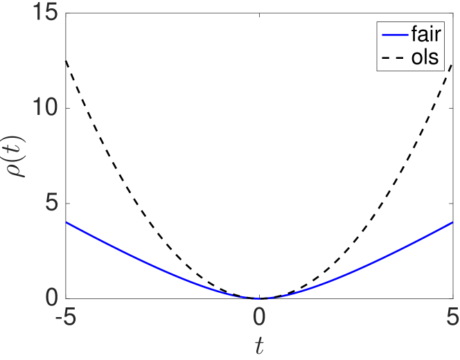
(a) Fair

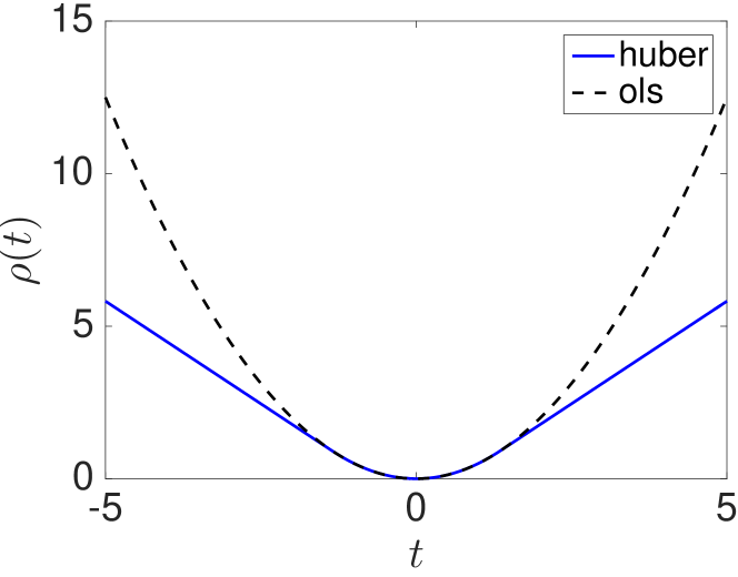
(b) Huber

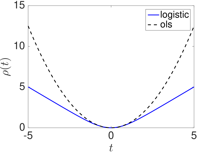
(c) logistic

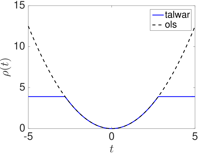
(d) Talwar

Figure 1: Loss functions Fair, Huber, logistic and Talwar for the tuning parameter $\beta$ corresponding to 95% efficiency (solid line) together with the standard loss function $t^{2}/2$ (dashed line).

2.3 Non-negativity constraints

In many applications, such as imaging, the reconstruction will benefit from taking into account the prior information about the component-wise non-negativity of the true solution $x_{\text{true}}$. Here, however, imposing non-negativity is not just a question of visual appeal, it also guarantees the two estimates (4) and (6) of the negative log-likelihood will provide similar results; see [31]. Therefore, the component-wise non-negativity constraint is an integral part of the resulting optimization problem. However, employment of the non-negativity constraint results in the need of more sophisticated optimization tools. The use of one of the possible algorithms is discussed in Section 4.

3 Regularization and selection of the regularization parameter

As a consequence of noise and ill-posedness of the inverse problem (1), some form of regularization needs to be employed in order to achieve a reasonable approximation of the true solution $x_{\text{true}}$. For computational convenience, we use Tikhonov regularization with a quadratic penalization term, i.e., we minimize the functional of the form

$$J_{\lambda}(x)\equiv\sum_{i=1}^{m}\rho\left(\frac{[Ax]_{i}-b_{i}}{\sqrt{[Ax]_{i}+\sigma^{2}}}\right)+\frac{\lambda}{2}\|Lx\|^{2},\qquad x\geq 0.$$ (16)

We assume that a good regularization parameter $\lambda$ with respect to $L$ is used so that the penalty term is reasonably close to the prior and the residual therefore is close to noise. In case of robust regression, it is particularly important not to over-regularize, since this would lead to large residuals and too many components of the data $b$ would be considered outliers. Methods for choosing $\lambda$ are discussed in this section.

3.1 Morozov’s discrepancy principle

Since the residual components are scaled, and for data without outliers we have the expected value

$$E\left\{\frac{1}{n}\sum_{i=1}^{n}\frac{([Ax]_{i}-b_{i})^{2}}{[Ax]_{i}+\sigma^{2}}\right\}=1,$$ (17)

an obvious choice would be to use the Morozov’s discrepancy principle [25, 32]. However, as reported in [31], even without outliers, the discrepancy principle based on (17) tends to provide unsatisfactory reconstructions for problems with large signal-to-noise ratio. Therefore we will not consider this approach further.

3.2 Generalized cross validation

The generalized cross validation method [11][32, chap. 7] is a method derived from the standard leave-one-out cross validation. To apply this method for linear Tikhonov regularization, one selects the regularization parameter $\lambda$ such that it minimizes the GCV functional

$$\text{GCV}(\lambda)=\frac{n\|r_{\lambda}\|^{2}}{(\text{trace}(I-A_{\lambda}))^{2}},$$ (18)

where $r_{\lambda}=Ax_{\lambda}-b=(A_{\lambda}-I)b$ is the residual, $n$ is its length, and the influence matrix $A_{\lambda}$ takes the form $A_{\lambda}=A(A^{T}A+\lambda L^{T}L)^{-1}A^{T}$. Here, due to the non-negativity constraints and the weights, the residual and the influence matrix have a more complicated form. An approximation of the influence matrix for problems with mixed noise, but without outliers, has been proposed in [1]. There the numerator of the GCV functional takes the form $n\|Wr_{\lambda}\|^{2}$ and the approximate influence matrix

$$A_{\lambda}=WA(D_{\lambda}(A^{T}W^{2}A+\lambda L^{T}L)D_{\lambda})^{\dagger}D_{\lambda}A^{T}W,$$ (19)

where $W$ and $D_{\lambda}$ are diagonal matrices:

$$W_{ii} =\frac{1}{\sqrt{[Ax_{\lambda}]_{i}+\sigma^{2}}};$$ (20)

$$[D_{\lambda}]_{ii} =\left\{\begin{array}[]{cc}1&[x_{\lambda}]_{i}>0,\\ 0&\text{otherwise,}\end{array}\right.$$ (23)

and  ^† denotes the Moore-Penrose pseudoinverse. Matrix $D_{\lambda}$ only handles the non-negativity constraints, and therefore can be adopted directly. The matrix $W$ needs a special adjustment, due to the change of the loss function to Talwar. The aim is to construct a matrix $W$ satisfying

$$\|Wr_{\lambda}\|^{2}=\sum_{i=1}^{m}\rho\left(\frac{[Ax_{\lambda}]_{i}-b_{i}}{\sqrt{[Ax_{\lambda}]_{i}+\sigma^{2}}}\right).$$

Substituting for $\rho$ from the definition of the function Talwar (14), we redefine the scaling matrix as

$$W_{ii} \equiv\left\{\begin{array}[]{cc}\frac{1}{\sqrt{[Ax_{\lambda}]_{i}+\sigma^{2}}}&\quad\left|\frac{[Ax_{\lambda}]_{i}-b_{i}}{\sqrt{[Ax_{\lambda}]_{i}+\sigma^{2}}}\right|\leq\beta,\\ \frac{\beta}{[Ax_{\lambda}]_{i}-b_{i}}&\text{otherwise};\end{array}\right.$$ (26)

In order to make the evaluation of (19) feasible for large-scale problems, we approximate the trace of a matrix using the random trace estimation [18, 32] as $\text{trace}(M)\approx v^{T}Mv$, where the entries of $v$ take values $\pm 1$ with equal probability. Applying the random trace estimation to (19), we obtain

$$(\text{trace}(I-A_{\lambda}))^{2}\approx(v^{T}v-v^{T}A_{\lambda}v)^{2}.$$

Finally, $A_{\lambda}v$ is approximated by $WAy$, with $y$ obtained applying truncated conjugate gradient iteration to

$$(D_{\lambda}(A^{T}W^{2}A+\lambda L^{T}L)D_{\lambda})y=D_{\lambda}A^{T}Wv.$$ (27)

4 Minimization problem

In this section we discuss numerical methods to compute a minimum of (16). We consider incorporating a non-negative constraint and solution of linear subproblems, including proposing a preconitioner.

4.1 Projected Newton’s method

Various methods for constrained optimization have been developed over the years, some related to image deblurring can be found in [2, 4, 14, 24, 28]. For our computations, we chose a projected Newton’s method, combined with projected PCG to compute the search direction in each step, see [13, sec. 6.4]. The convenience of this method lies in the fact that the projected PCG does not require any special form of the preconditioner and a generic conjugate gradient preconditioner can be employed. Besides lower bounds, upper bounds on the reconstruction can also be enforced. For completeness, we include the projected Newton method in Algorithm 1, and projected PCG in Algorithm 2.

Algorithm 1 Projected Newton’s method [13]

  $k=0$

  while not converged do

     $\text{Active}=(x^{(k)}\leq 0$)

     $g=\text{grad}_{J_{\lambda}}(x^{(k)})$

     $H=\text{Hess}_{J_{\lambda}}(x^{(k)})$

     $M=\texttt{prec}(H)$ {setup preconditioner for the Hessian}

     $s=\texttt{projPCG}(H,-g,\text{Active},M)$ {compute the search direction for inactive cells}

     $g_{a}=g(\text{Active})$

     if $\max(\text{abs}(g_{a}))>\max(\text{abs}(s))$ then

        $g_{a}=g_{a}\cdot\max(\text{abs}(s))/\max(\text{abs}(g_{a}))$ {rescaling needed}

     end if

     $s(\text{Active})=g_{a}$ {take gradient direction in active cells}

     $x^{(k+1)}=\texttt{linesearch}(s,x^{(k)},J_{\lambda},\text{grad}_{J_{\lambda}})$

     $k=k+1$

  end while

  return  $x^{(k)}$

Algorithm 2 Projected PCG [13]

  input: $A$, $b$, Active, $M$

  $x_{0}=0$

  $D_{\mathcal{I}}=\text{diag}(1-\text{Active})$ {projection onto inactive set}

  $r_{0}=D_{\mathcal{I}}b$

  $z_{0}=D_{\mathcal{I}}(M^{-1}r_{0})$

  $p_{0}=z_{0}$

  $k=0$

  while not converged do

     $\alpha_{k}=\frac{r_{k}^{T}z_{k}}{p^{T}D_{\mathcal{I}}Ap_{k}}$

     $x_{k+1}=x_{k}+\alpha_{k}p_{k}$

     $r_{k+1}=x_{k}-\alpha_{k}D_{\mathcal{I}}Ap_{k}$

     $z_{k+1}=D_{\mathcal{I}}(M^{-1}r_{k})$

     $\beta_{k+1}=\frac{z_{k+1}^{T}r_{k+1}}{z_{k}^{T}r_{k}}$

     $p_{k+1}=z_{k+1}+\beta_{k}p_{k}$

     $k=k+1$

  end while

  return  $x_{k}$

4.2 Solution of the linear subproblems

Each step of the projected Newton method (Algorithm 1) requires solving a linear system with the Hessian:

$$\text{Hess}_{J_{\lambda}}(x^{(k)})s =-\text{grad}_{J_{\lambda}}(x^{(k)})$$

$$(A^{T}D^{(k)}A+\lambda L^{T}L)s =-\left(A^{T}z^{(k)}+\lambda L^{T}Lx^{(k)}\right).$$ (28)

For the objective functional (16), the diagonal matrix $D^{(k)}$ and the vector $z^{(k)}$ have the form:

$$z_{i} =\left\{\begin{array}[]{ll}\frac{1}{2}\left(1-\frac{\left(b_{i}+\sigma^{2}\right)^{2}}{\left([Ax]_{i}+\sigma^{2}\right)^{2}}\right),&\left|\frac{[Ax]_{i}-b_{i}}{\sqrt{[Ax]_{i}+\sigma^{2}}}\right|\leq\beta,\\ 0,&\text{otherwise}.\end{array}\right.$$ (31)

$$D_{ii} =\left\{\begin{array}[]{ll}\frac{\left(b_{i}+\sigma^{2}\right)^{2}}{\left([Ax]_{i}+\sigma^{2}\right)^{3}},&\left|\frac{[Ax]_{i}-b_{i}}{\sqrt{[Ax]_{i}+\sigma^{2}}}\right|\leq\beta,\\ 0,&\text{otherwise}.\end{array}\right.$$ (34)

Note that in case of constant weights, robust regression represents extra computational cost in comparison with standard least squares because it leads to a sequence of weighted least squares problems, while standard least squares problems are solved in one step. In our setting, the weights in (6) themselves have to be updated and therefore employing a different loss function does not change the type of the problem we need to solve.

Without preconditioning, the convergence of projected PCG can be rather slow, and it is therefore important to consider preconditioning. The idea of many preconditioners, such as constraint [19, 8], constraint-type [7] or Hermitian and skew-Hermitian [3] preconditioners is based on the fact that in many cases it is possible to efficiently solve the linear system in (28) if the diagonal matrix $D^{(k)}$ is the identity matrix; that is, if the linear system involves the matrix

$$A^{T}A+\lambda L^{T}L.$$ (35)

For example, in the case of image deblurring, it is well known that linear systems involving the matrix (35) can be solved efficiently using fast trigonometric or fast Fourier transforms (FFT).

Although the constraint-type, and Hermitian and skew-Hermitian preconditioners seem to perform well for problems with a random matrix $D^{(k)}$ (i.e., a random row scaling), see [3], they performed unsatisfactorily for problems of the form (28), (34).

A preconditioner based on a similar idea of fast computations with matrices of type (35) for imaging problems was proposed in [10]. In this case, the row scaling is approximated by a column scaling; that is, we find $\hat{D}^{(k)}$ such that

$$A^{T}D^{(k)}A\approx\hat{D}^{(k)}(A^{T}A)\hat{D}^{(k)},$$ (36)

where

$$\hat{D}_{ii}^{(k)}\equiv\sqrt{\frac{e_{i}^{T}(A^{T}D^{(k)}A)e_{i}}{e_{i}^{T}(A^{T}A)e_{i}}}.$$ (37)

Note that for $\hat{D}^{(k)}$ defined in (37), the diagonals of the matrices on the two sides of approximation (36) are exactly equal.

Since for large-scale problems, matrix $A$ is typically not formed explicitly, exact evaluation of the entries of $\hat{D}^{(k)}$ might become too expensive. To get around this restriction, note that

$$e_{i}^{T}(A^{T}D^{(k)}A)e_{i}=((A^{T})\,.^{2}\,\text{diag}(D^{(k)}))_{i}\quad\text{and}\quad e_{i}^{T}(A^{T}A)e_{i}=((A^{T})\,.^{2}\,\mathbf{1})_{i},$$ (38)

where $\mathbf{1}$ a vector of all ones, and we use MATLAB notation $.^{2}$ to mean component-wise squaring. In some cases it may be relatively easy to compute both the entries of $(A^{T}).^{2}$ and the vector $(A^{T}).^{2}\mathbf{1}$; this is the case for image deblurring, and is discussed in more detail in Section 5.

Using (36), we define the preconditioner for the linear system (28) as

$$M\equiv\hat{D}^{(k)}\left(A^{T}A+\hat{\lambda}L^{T}L\right)\hat{D}^{(k)},$$ (39)

with

$$\hat{\lambda}\equiv\lambda/\text{mean}\left(\text{diag}(\hat{D}^{(k)})\right)^{2}.$$

More details on the computational costs involved in constructing and applying the preconditioner in the case of image deblurring are provided in Section 5.

5 Numerical tests

The Poisson–Gaussian model arises naturally in image applications, so in this section we present numerical examples from image deblurring. Specifically, we consider the inverse problem (1) with data model (2), where vector $b$ is an observed image that is corrupted by blur and noise, matrix $A$ models the blurring operation, vector $x_{\text{true}}$ is the true image, and $\eta$ is noise. Although an image is naturally represented as an array of pixel values, when we refer to ‘vector’ representations, we assume the pixel values have been reordered as vectors. For example, if we have a $p\times p$ image of pixel values, these can be stored in a vector of length $n=p^{2}$ by, for example, lexicographical ordering of the pixel values.

In many practical image deblurring applications, the blurring is spatially invariant, and $A$ is structured matrix defined by a point spread function (PSF). In this situation, image deblurring can also be referred to as image decovolution, because the operation $Ax_{\text{true}}$ is the convolution of $x_{\text{true}}$ and the PSF. Although the PSF may be given as an actual function, the more common situation is to compute estimates of it by imaging point source objects. Thus, the PSF can be represented as an image; we typically display the PSF as a mesh plot, which makes it easier to visualize how a point in an image is spread to its neighbors because of the blurring operation. The precise structure of the matrix $A$ depends on the imposed boundary condition; see [16] for details. In this section we impose periodic boundary conditions, so that $A$ and $L$ are both diagonalizable by FFTs.

So far we have only described what we refer to as the single-frame situation, where $b$ is a single observed image. It is often the case, especially in astronomical imaging, to have multiple observed images of the same object, but with each having a different blurring matrix associated with it. We refer to this as the multi-frame image deblurring problem. Here, $b$ represents all observed images, stacked one on top of each other, and similarly $A$ is formed by stacking the various blurring matrices.

Before describing the test problems used in this section, we first summarize the computational costs. From the discussion around equation (38), to construct the preconditioner we need to be able to efficiently square all entries of the matrix $A^{T}$, or equivalently those of $A$; this can easily be approximated by squaring the point-spread function component-wise before forming the operator, i.e.,

$$(A_{\text{PSF}}).^{2}\approx A_{\text{PSF}.^{2}}\,.$$ (40)

Using this approximation, in each Newton step we only need to perform one multiplication by a matrix, one component-wise multiplication, and one component-wise square-root to obtain the entries of the diagonal matrix (37). With the assumption that $A$ and $L$ are both diagonalizable by FFTs, efficient multiplication by the Hessian (28) involves two two-dimensional forward and inverse FFTs, which we refer to as fft2 and ifft2, respectively. Solving systems with matrix (39) involves only one fft2 and one ifft2. In addition to the fft2 requirements, multiplication by the Hessian (28) involves 4 pixel-wise multiplications and 1 addition. Solving systems with the preconditioner (39) involves 3 pixel-wise multiplications (component-wise reciprocals are assumed to be computed only once at the beginning). The total counts for each operation are shown in Table 1.

Table 1: Operation counts for single-frame case.

	operation	fft2	ifft2	mults	adds
Hessian (28)	multiply	2	2	4	1
preconditioner (39)	solve	1	1	3	0

The robustness and the efficiency of the proposed method is demonstrated on two test problems adopted from [27]:

Satellite

An atmospheric seeing problem with spatially invariant atmospheric blur (moderate seeing conditions with the Fried parameter 30). We also consider a multi-frame case, where the same object is blurred by three different PSFs. These PSFs are generated by transposing and flipping the first PSF. The setting is shown in Figures 2 and 4(a).

Carbon ash

An image deblurring problem with spatially invariant non-separable Gaussian blur, where the PSF has the functional definition

$$\mbox{PSF}(s,t)=\frac{1}{2\pi\sqrt{\gamma}}\exp\left\{-\frac{1}{2}\left[\begin{array}[]{cc}s&t\end{array}\right]C^{-1}\left[\begin{array}[]{c}s\\ t\end{array}\right]\right\}\,,$$ (41)

where

$$C=\left[\begin{array}[]{cc}\gamma_{1}^{2}&\tau^{2}\\[3.0pt] \tau^{2}&\gamma_{2}^{2}\end{array}\right]\,,\quad\mbox{and}\quad\gamma_{1}^{2}\gamma_{2}^{2}-\tau^{4}>0\,.$$

The shape of the Gaussian PSF depends on the parameters $\gamma_{1},\gamma_{2}$ and $\tau$; we use $\gamma_{1}=4$, $\gamma_{2}=2$; $\tau=2$. We also consider a multi-frame case, where the same object is blurred by three different PSFs. The other two PSFs are Gaussian blurs with parameters $\gamma_{1}=4$, $\gamma_{2}=2$, $\tau=0$, and $\gamma_{1}=4$, $\gamma_{2}=2$, $\tau=0$. The setting is shown in Figures 3 and 4(b).

As previously mentioned, in the multi-frame case, the vector $b$ in (1) is concatenation of the vectorized blurred noisy images, the matrix $A$ is concatenation of the blurring operators, i.e., $A\in\mathbb{R}^{3n\times n}$. For the test problems all true images are $256\times 256$ arrays of pixels (with intensities scaled to $[0,255]$), and thus $n=65536$.

Computation was performed in MATLAB R2015b. Noise is generated artificially using MATLAB functions poissrnd and randn. Unless specified otherwise, the standard deviation $\sigma$ is set to $5$. We use the discretized Laplacian, see [16, p. 95], as the regularization matrix $L$. The Projected Newton method (Algorithm 1) is terminated when the relative size of the projected gradient

$$\mathcal{P}(\text{grad}_{J_{\lambda}}(x^{(k)})),\quad\text{where}\quad\mathcal{P}(v)\equiv v.*(1-\text{Active})+\text{Active}.*(v<0),$$ (42)

reaches the tolerance $10^{-4}$ or after 40 iterations. We use MATLAB notation $.^{*}$ to mean component-wise multiplication. Projected PCG (Algorithm 2) is terminated when the relative size of the projected residual (denoted in Algorithm 2 by $r_{i}$) reaches $10^{-1}$, or the number of iterations reaches $100$. We use the preconditioner given in (39) as the default preconditioner. Given a search direction $s_{k}$, we apply a projected backtracking linesearch, with the initial step length equal to 1, which we terminate when

$$J_{\lambda}(x^{(k+1)})<J_{\lambda}(x^{(k)}).$$

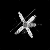
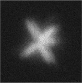
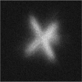
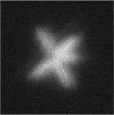
Figure 2: Test problem Satellite: true image (left) together with three blurred noisy images (right).

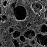
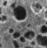
Figure 3: Test problem Carbon ash: true image (left) together with three blurred noisy images (right).

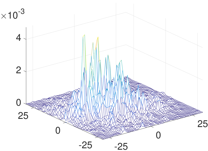
(a) Satellite

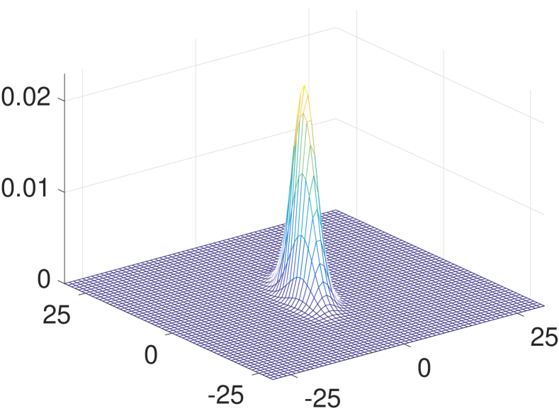
(b) Carbon ash

Figure 4: Point-spread functions for the first frame of each test problem.

5.1 Robustness with respect to various types of outliers

In this section, we consider several types of outliers, whose choice was motivated by [5], and demonstrate the robustness of the proposed method. Note that the difference between [5] and the proposed approach lies, among others, in the fact that while in [5], the approximation of the solution is computed in order to update the outer (robust) weights associated with the components of residual. Here, the weights are represented by the loss function $\rho$ and are updated implicitly in each Newton step and therefore our approach does not involve any outer iteration.

Random corruptions

First we consider the most simple case of the outliers – a given percentage of pixels is corrupted at random. These corruptions are generated artificially by adding a value randomly chosen between $0$ and $\max(Ax_{\text{true}})$ to the given percentage of pixels. The location of these pixels is also chosen randomly. Figures 5(a), 5(b), 5(c), and 5(d) show semiconvergence curves, representing the dependence of the error on the regularization parameter $\lambda$, when we increase the percentage of corrupted pixels.

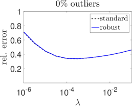
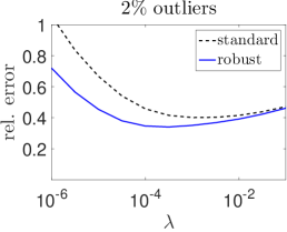
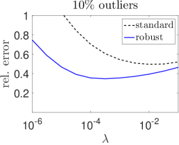
(a) Satellite single-frame

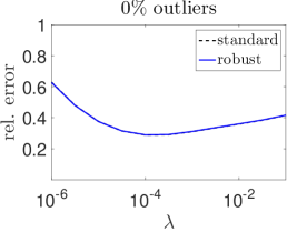
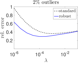
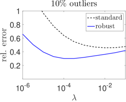
(b) Satellite multi-frame

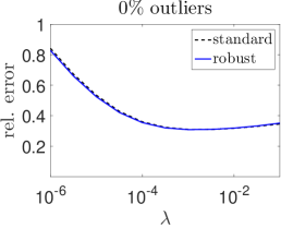
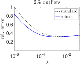
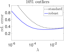
(c) Carbon ash single-frame

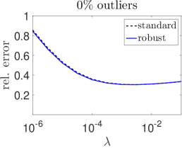
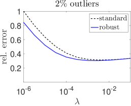
(d) Carbon ash multi-frame

Figure 5: Semiconvergence curves – dependence of the relative error of the reconstruction on the size of the regularization parameter $\lambda$ for various percentages of outliers: Talwar (10) - (15) (solid line) and the standard data fidelity function (6) (dashed line).

It is no surprise that when outliers occur, more regularization is needed in order to obtain a reasonable approximation of the true image $x_{\text{true}}$. This is however not the case if we use loss function Talwar, for which the semiconvergence curve remains the same even with increasing percentage of outliers, and therefore no adjustment of the regularization parameter is needed. In Figures 6 and 7, we show the reconstructions corresponding to $10\%$ outliers. The regularization paramter is chosen as a close-to-the-optimal regularization parameter for the same problem with no outliers. Note that Figures 6 and 7 show only one frame for illustration. In the multi-frame case, the corruptions look similar for all frames, except that the random locations of the outliers is different. For random outliers like this, robust regression is clearly superior to standard weighted least squares. The influence of the outliers in the multi-frame case is less severe, due to intrinsic regularization of the overdetermined system (1). A more comprehensive comparison of the standard and robust approach is shown in Table 2, giving the percentage of cases in which the robust approach provides better reconstruction. The robust approach provides better reconstruction in all cases except for the test problem Satellite with no outliers, where the standard approach gave sometimes slightly better reconstructions. However, even in these cases we observed that the difference between the errors of the reconstructions is rather negligible, about $3\%$.

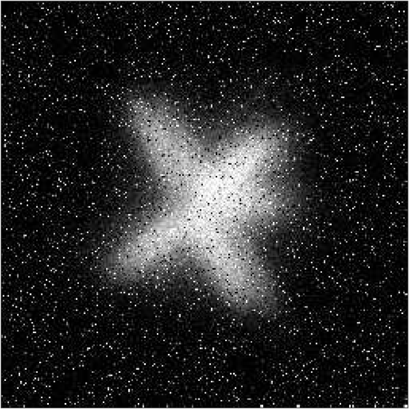
(a) data

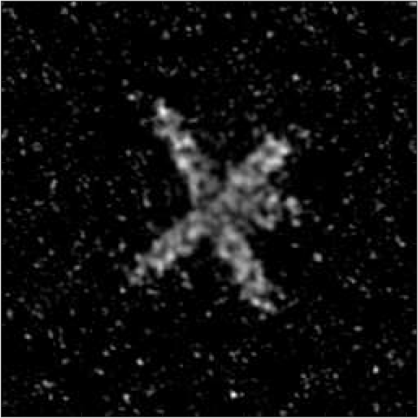
(b) single-frame
standard

(c) single-frame
robust

(d) multi-frame,
standard

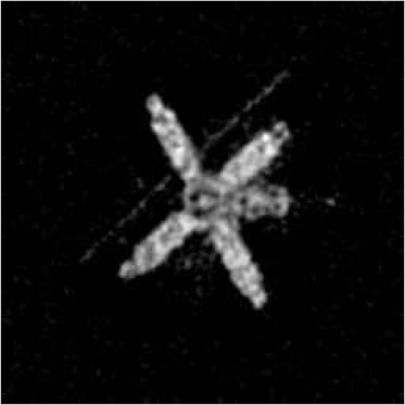
(e) multi-frame
robust

Figure 6: Random corruptions: (a) blurred noisy image with $10\%$ corrupted pixels (only first frame is shown); (b) - (d) reconstructions corresponding to $\lambda=10^{-4}$.

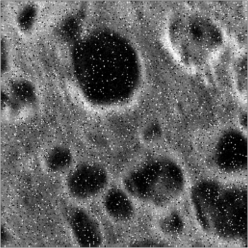
(a) data

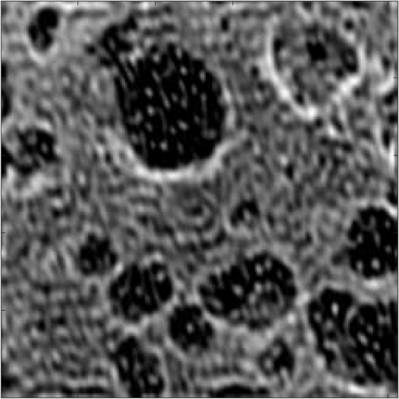
(b) single-frame
standard

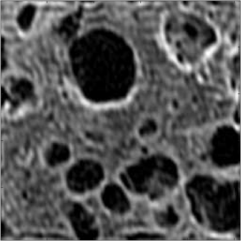
(c) single-frame
robust

(d) multi-frame,
standard

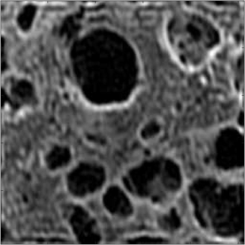
(e) multi-frame
robust

Figure 7: Random corruptions: (a) blurred noisy image with $10\%$ corrupted pixels (only first frame is shown); (b) - (d) reconstructions corresponding to $\lambda=10^{-3}$.

Table 2: Comparison of the quality of reconstruction for the standard vs. the robust approach. For each test problem and each percentage of outliers, the results are averaged over 100 independent positions and sizes of random corruptions. Regularization parameters are chosen identically as in Figures 6 and 7. Reconstructions are considered to be of the same quality if the difference between the corresponding relative errors is smaller than 1%.

better reconstruction: robust/same/standard
problem/% outliers	0%	1%	2%	5%
Satellite single-frame	0/93/7	100/0/0	100/0/0	100/0/0
Satellite multi-frame	0/94/6	100/0/0	100/0/0	100/0/0
Carbon ash single-frame	0/100/0	100/0/0	100/0/0	100/0/0
Carbon ash multi-frame	0/100/0	100/0/0	100/0/0	100/0/0

Added object with different blurring

We also consider a situation when a small object appears in the scene, but is blurred by a different PSF than the main object (satellite). The aim is to recover the main object, while suppressing the influence of the added one. In our case, the added object is a small satellite in the left upper corner that is blurred by a small motion blur. In the multi-frame case, the small satellite is added to the first frame only. The difference between the reconstructions using standard and robust approach is shown in Figure 8. For the single frame problem, reconstructions obtained using the standard loss function is fully dominated by the small added object. For the multi-frame situation, the influence of the outlier is somewhat compensated by the two frames without outliers. In both cases, however, robust regression provides better reconstruction, comparable to the reconstruction from the data without outliers.

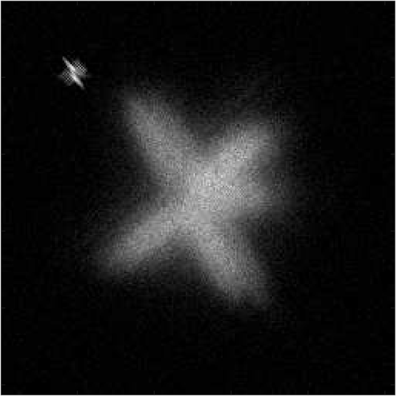
(a) data

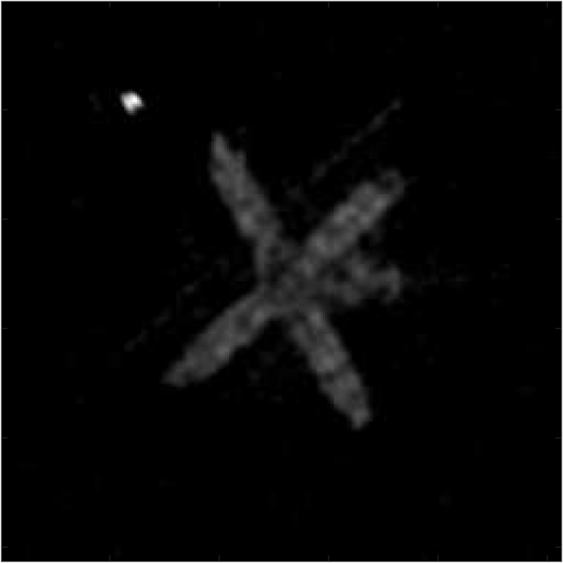
(b) single-frame
standard

(c) single-frame
robust

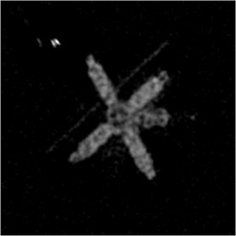
(d) multi-frame,
standard

(e) multi-frame
robust

Figure 8: Added object: (a) blurred noisy image with a small object added to the first frame (only first frame is shown); (b) - (d) reconstructions corresponding to $\lambda=10^{-4}$.

Outliers introduced by boundary conditions

Defining the boundary conditions plays an important role in solving image deblurring problems. As is well known, see e.g. [16], unless some strong a priori information about the scene outside the borders is available, any choice of the boundary conditions may lead to artefacts around edges in the reconstruction. Similarly as in [5], we may expect that the robust objective functional (16) can to some extent compensate for these edge artifacts, i.e., the outliers are represented by the ‘incorrectly’ imposed boundary conditions. In our model we assume periodic boundary conditions, which is computationally very appealing, since it allows evaluating the multiplication by $A$ very efficiently using the fast Fourier transform. However, if any of the objects in the scene is close to the boundary, these boundary conditions will most probably cause artifacts. In order to demonstrate the ability of the proposed scheme to eliminate influence of this type of outlier, we shifted the satellite to the right edge of the image. Other settings remain unchanged. Reconstructions using standard and robust approach are shown in Figure 9. We see that, although not spectacular, robust regression can reduce the artifacts caused by incorrectly imposed boundary conditions and therefore provide better reconstruction of the true image. Quantitative results for this and all the previous types of outliers are shown in Tables 3(a) and 3(b).

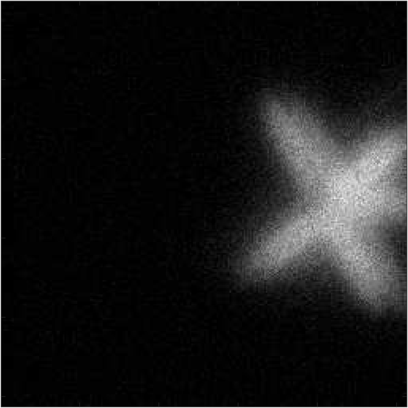
(a) data

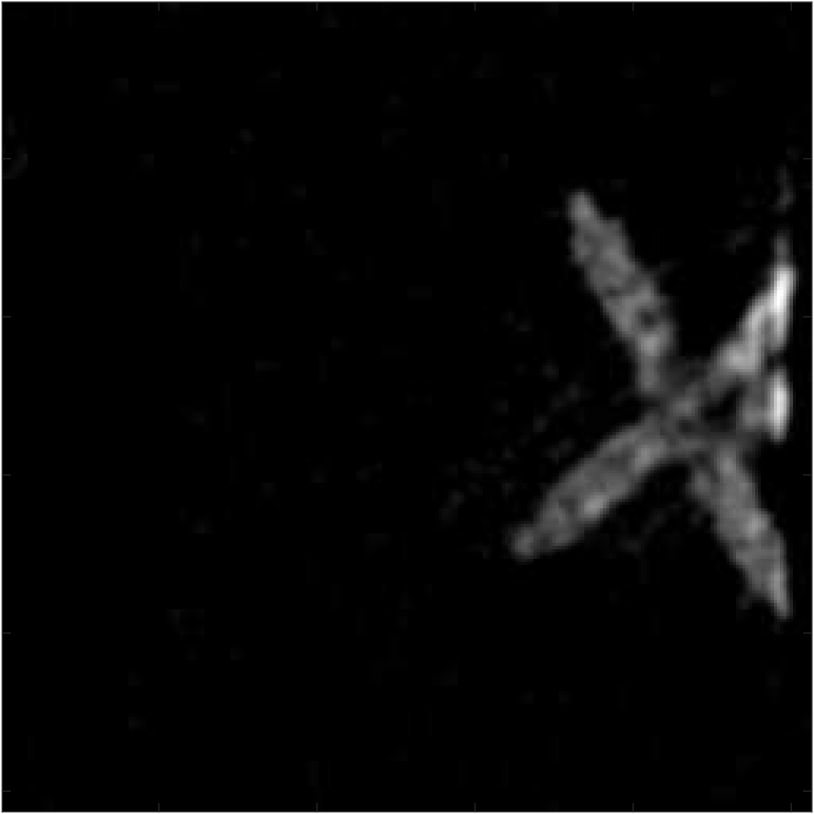
(b) single-frame
standard

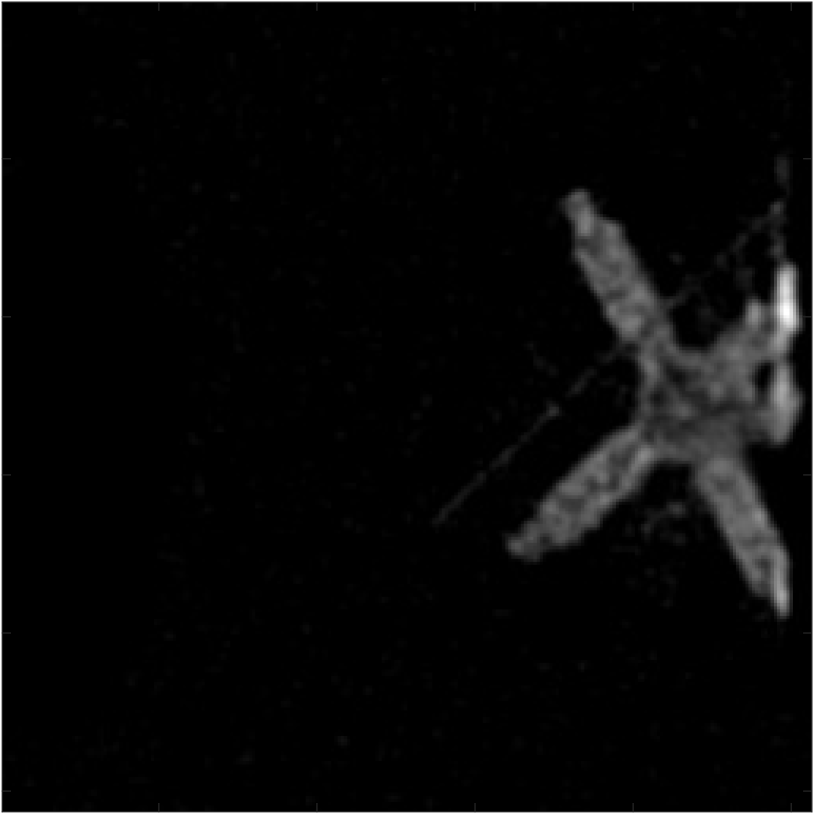
(c) single-frame
robust

(d) multi-frame,
standard

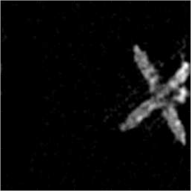
(e) multi-frame
robust

Figure 9: Incorrectly imposed periodic boundary conditions: (a) blurred noisy image close to the edge (only first frame is shown); (b) - (d) reconstructions corresponding to $\lambda=10^{-4}$.

Table 3: Comparison of the standard and robust approach in terms of relative error of the reconstruction. Each row contains results for the standard and robust approach. Abbreviation ‘# it’ stands for the number of Newton steps performed before the relative size of the projected gradient reached the tolerance $10^{-4}$. Corresponding reconstructions are shown in Figures 6–9.

(a) single-frame

	standard		robust
problem	# it	rel. error	# it	rel. error
Satellite	15	3.40$\times 10^{-1}$	16	3.42$\times 10^{-1}$
Satellite random corr. 10%	14	6.78$\times 10^{-1}$	14	3.57$\times 10^{-1}$
Carbon ash	10	3.10$\times 10^{-1}$	11	3.08$\times 10^{-1}$
Carbon ash random corr. 10%	11	3.80$\times 10^{-1}$	14	3.10$\times 10^{-1}$
Satellite added object	15	4.72$\times 10^{-1}$	15	3.43$\times 10^{-1}$
Satellite boundary conditions	15	5.48$\times 10^{-1}$	25	4.51$\times 10^{-1}$

(b) multi-frame

	standard		robust
problem	# it	rel. error	# it	rel. error
Satellite	12	2.89$\times 10^{-1}$	11	2.89$\times 10^{-1}$
Satellite random corr. 10%	11	6.45$\times 10^{-1}$	13	3.00$\times 10^{-1}$
Carbon ash	12	3.07$\times 10^{-1}$	11	3.05$\times 10^{-1}$
Carbon ash random corr. 10%	9	3.70$\times 10^{-1}$	19	3.06$\times 10^{-1}$
Satellite added object	13	3.33$\times 10^{-1}$	11	2.90$\times 10^{-1}$
Satellite boundary conditions	14	5.26$\times 10^{-1}$	14	4.27$\times 10^{-1}$

5.2 Generalized cross-validation

For the remainder of this section we will only assume the robust approach, i.e., functional (16) with the loss function Talwar. In Section 3.2 we described a regularization parameter selection rule based on leave-one-out cross validation. Since GCV belongs to standard methods, we focus here mainly on the influence of the outliers on its reliability. To obtain various noise levels, we scale the original true scene (with maximum intensity = 255) by 10 and by 100, which results in a decrease of the relative size of Poisson noise. The standard deviation $\sigma$ for the additive Gaussian noise is scaled accordingly by $\sqrt{10}$ and $10$. We compute the resulting signal-to-noise ratio as the reciprocal of the coefficient of variation, i.e.,

$$\text{SNR}=\frac{\|Ax\|}{\sqrt{\sum_{i=1}^{n}([Ax]_{i}+\sigma^{2})}}.$$

For our computations, we use CG to solve (27), which we terminate if the relative size of the residual reaches $10^{-4}$ or if the number of iterations reaches 150. To minimize the GCV functional, we use the MATLAB built-in function fminbnd, for which we set the lower bound to $0$ and the upper bound to $10^{-1}$, $10^{-2}$, $10^{-4}$, depending on the maximum intensity of the image. The tolerance TolX was set to $10^{-8}$.

For test problem Satellite, we show the semiconvergence curves including the minimum error and the error obtained using GCV in Figure 10. Quantitative results (averaged over 10 realizations of outliers) for both test problems are shown in Table 4. We observe that the proposed rule is rather stable with respect to the increasing number of outliers and generally better for the Carbon ash than for the Satellite. As expected, the method provides better approximation of the optimal regularization parameter for smaller noise levels (larger $Ax_{\text{true}}$), where the functional (6) approximates better the maximum likelihood functional for the mixed Poisson–Gaussian model. Occasionally, GCV provides slightly worse reconstruction for the highest percentage (10%) of outliers.

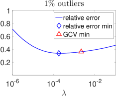
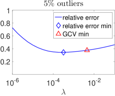
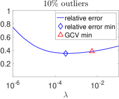
(a) Satellite single-frame, max. intensity 255 (SNR = 5).

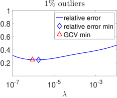
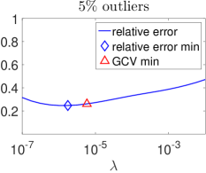
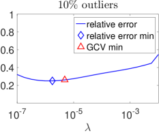
(b) Satellite single-frame, max. intensity 2550 (SNR = 17).

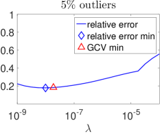
(c) Satellite single-frame, max. intensity 25500 (SNR = 52).

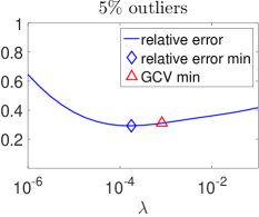
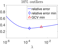
(d) Satellite multi-frame, max. intensity 255 (SNR = 5).

Figure 10: GCV for data with outliers.

Table 4: Relative errors of the reconstruction: optimal $\lambda$ vs. $\lambda$ obtained by minimizing the GCV functional (18).

(a) Satellite

		error min			($\lambda$ optimal)
		error GCV			($\lambda$ GCV)
	% outliers
problem	max. int.	1%		5%		10%
single-frame	255	$3.39\times 10^{-1}$	($\lambda_{\text{opt}}=2.1\times 10^{-4}$)	$3.43\times 10^{-1}$	($\lambda_{\text{opt}}=2.5\times 10^{-4}$)	$3.49\times 10^{-1}$	($\lambda_{\text{opt}}=3.2\times 10^{-4}$)
		$3.60\times 10^{-1}$	($\lambda_{\text{GCV}}=2.1\times 10^{-3}$)	$3.68\times 10^{-1}$	($\lambda_{\text{GCV}}=3.1\times 10^{-3}$)	$3.80\times 10^{-1}$	($\lambda_{\text{GCV}}=5.6\times 10^{-3}$)
single-frame	2550	$2.46\times 10^{-1}$	($\lambda_{\text{opt}}=1.5\times 10^{-6}$)	$2.48\times 10^{-1}$	($\lambda_{\text{opt}}=1.5\times 10^{-6}$)	$2.50\times 10^{-1}$	($\lambda_{\text{opt}}=1.7\times 10^{-6}$)
		$2.48\times 10^{-1}$	($\lambda_{\text{GCV}}=1.5\times 10^{-6}$)	$2.57\times 10^{-1}$	($\lambda_{\text{GCV}}=4.5\times 10^{-6}$)	$2.69\times 10^{-1}$	($\lambda_{\text{GCV}}=8.4\times 10^{-6}$)
single-frame	25500	$1.78\times 10^{-1}$	($\lambda_{\text{opt}}=1.0\times 10^{-8}$)	$1.79\times 10^{-1}$	($\lambda_{\text{opt}}=1.0\times 10^{-8}$)	$1.81\times 10^{-1}$	($\lambda_{\text{opt}}=1.0\times 10^{-8}$)
		$1.79\times 10^{-1}$	($\lambda_{\text{GCV}}=8.8\times 10^{-9}$)	$1.81\times 10^{-1}$	($\lambda_{\text{GCV}}=1.5\times 10^{-8}$)	$2.42\times 10^{-1}$	($\lambda_{\text{GCV}}=7.5\times 10^{-6}$)
mutli-frame	255	$2.89\times 10^{-1}$	($\lambda_{\text{opt}}=1.8\times 10^{-4}$)	$2.92\times 10^{-1}$	($\lambda_{\text{opt}}=1.8\times 10^{-4}$)	$2.97\times 10^{-1}$	($\lambda_{\text{opt}}=1.8\times 10^{-4}$)
		$3.16\times 10^{-1}$	($\lambda_{\text{GCV}}=1.6\times 10^{-3}$)	$3.13\times 10^{-1}$	($\lambda_{\text{GCV}}=1.2\times 10^{-3}$)	$3.49\times 10^{-1}$	($\lambda_{\text{GCV}}=5.8\times 10^{-3}$)

(b) Carbon ash

		error min			($\lambda$ optimal)
		error GCV			($\lambda$ GCV)
	% outliers
problem	max. int.	1%		5%		10%
single-frame	255	$3.08\times 10^{-1}$	($\lambda_{\text{opt}}=1.8\times 10^{-3}$)	$3.09\times 10^{-1}$	($\lambda_{\text{opt}}=1.8\times 10^{-3}$)	$3.10\times 10^{-1}$	($\lambda_{\text{opt}}=1.7\times 10^{-3}$)
		$3.12\times 10^{-1}$	($\lambda_{\text{GCV}}=8.9\times 10^{-4}$)	$3.11\times 10^{-1}$	($\lambda_{\text{GCV}}=1.5\times 10^{-3}$)	$3.11\times 10^{-1}$	($\lambda_{\text{GCV}}=2.2\times 10^{-3}$)
single-frame	2550	$2.91\times 10^{-1}$	($\lambda_{\text{opt}}=1.9\times 10^{-5}$)	$2.92\times 10^{-1}$	($\lambda_{\text{opt}}=2.1\times 10^{-5}$)	$2.92\times 10^{-1}$	($\lambda_{\text{opt}}=1.9\times 10^{-5}$)
		$2.97\times 10^{-1}$	($\lambda_{\text{GCV}}=9.7\times 10^{-6}$)	$2.95\times 10^{-1}$	($\lambda_{\text{GCV}}=1.2\times 10^{-5}$)	$2.93\times 10^{-1}$	($\lambda_{\text{GCV}}=2.2\times 10^{-5}$)
single-frame	25500	$2.77\times 10^{-1}$	($\lambda_{\text{opt}}=3.0\times 10^{-7}$)	$2.78\times 10^{-1}$	($\lambda_{\text{opt}}=2.7\times 10^{-7}$)	$2.79\times 10^{-1}$	($\lambda_{\text{opt}}=2.6\times 10^{-7}$)
		$3.00\times 10^{-1}$	($\lambda_{\text{GCV}}=5.2\times 10^{-8}$)	$2.84\times 10^{-1}$	($\lambda_{\text{GCV}}=9.4\times 10^{-8}$)	$2.82\times 10^{-1}$	($\lambda_{\text{GCV}}=1.3\times 10^{-7}$)
multi-frame	255	$3.03\times 10^{-1}$	($\lambda_{\text{opt}}=1.8\times 10^{-3}$)	$3.04\times 10^{-1}$	($\lambda_{\text{opt}}=1.8\times 10^{-3}$)	$3.04\times 10^{-1}$	($\lambda_{\text{opt}}=1.8\times 10^{-3}$)
		$3.14\times 10^{-1}$	($\lambda_{\text{GCV}}=6.8\times 10^{-4}$)	$3.07\times 10^{-1}$	($\lambda_{\text{GCV}}=9.8\times 10^{-4}$)	$3.05\times 10^{-1}$	($\lambda_{\text{GCV}}=1.9\times 10^{-3}$)

5.3 Linear subproblems

As mentioned earlier, various types of preconditioners have been developed to speed up convergence of iterative methods applied to systems of type (28) or its saddle-point counterpart

$$\begin{pmatrix}D^{-1}&A\\ A^{T}&\lambda L^{T}L\\ \end{pmatrix}=\begin{pmatrix}-z\\ \lambda L^{T}Lx\\ \end{pmatrix}.$$

The Hermitian and skew-Hermitian (HSS) preconditioner, as well as constraint precondtioner belong to the best known preconditioners for this type of linear system. Both were incorporated in GMRES and tested on deblurring problems with random diagonal scaling $D$ in [3]. Using random $D$, they indeed accelerate convergence also in our case, as shown in Figure 11. However, our preconditioner (39) provides a much better speedup. Moreover, for real computations, e.g., when the matrix $D$ is actually generated during the Projected Newton computation, the HSS and constraint preconditioners did not perform well, and even slowed down the convergence, see Figure 12. This is fortunately not the case for our proposed preconditioner. In this experiment, we did not assume projection on the non-negative half-plane and since in (5.3), we need to evaluate $D^{-1}$, if some component $D_{ii}=0$, we replaced it by $2\sqrt{\epsilon_{\text{mach}}}$, see also [23]. We also did not incorporate any outliers for these initial experiments with the preconditioners; these results are intended to show that our proposed preconditioning for these problems often performs much better than the well-known standard preconditioners. In fact, we see that the behavior of the constraint and HSS preconditioner depends heavily on the actual setting of the problem. In the remainder of this section we will therefore focus on the preconditioner given in (39).

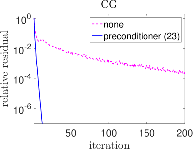
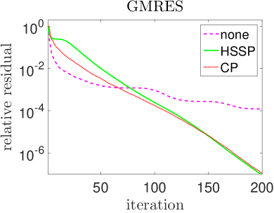
(a) Satellite single-frame, random diagonal

Figure 11: Preconditoner defined in (39), constraint preconditioner (CP), and Hermitian and skew-Hermitian splitting preconditioner (HSSP) performance for $(A^{T}DA+\lambda L^{T}L)s=-A^{T}b$, where $A$ and $b$ are adopted from the test problem Satellite, and $D$ is a diagonal with random entries uniformly distributed in $(0,1)$.

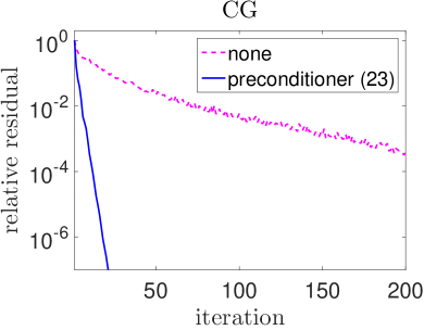
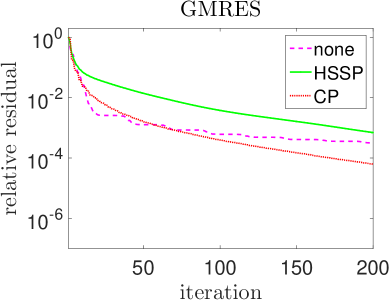
(a) Satellite single-frame, Newton it = 3

Figure 12: Preconditoner defined in (39), constraint preconditioner (CP), and Hermitian/skew-Hermitian preconditioner (HSSP) performance for $(A^{T}D^{(k)}A+\lambda L^{T}L)s=-\left(A^{T}z^{(k)}+\lambda L^{T}Lx^{(k)}\right)$.

In Figure 13, we investigate the overall speedup of the convergence by plotting the number of projected PCG steps needed in each Newton iteration to reach the desired tolerance on the relative size of the projected gradient. Even for the most generous tolerance $10^{-1}$, preconditioner (39) significantly reduces the number of projPCG iterations. Note that in this experiment, the linear subproblems solved in each Newton iteration are generally not identical, since the subproblems are not solved exactly and therefore the approximations $x^{(k)}$ are not the same. We set the outer tolerance to $0$ in order to perform always at least $15$ Newton iterations.

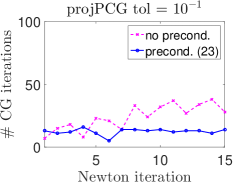
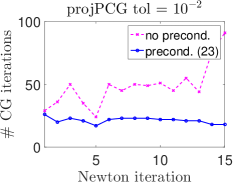
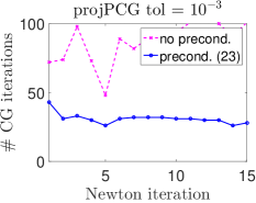
(a) Satellite single-frame

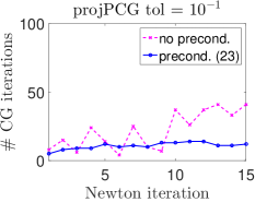
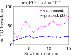
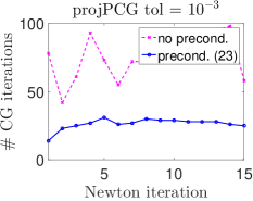
(b) Satellite multi-frame

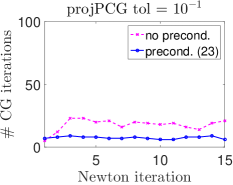
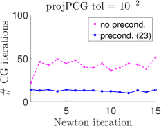
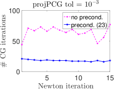
(c) Carbon Ash single-frame

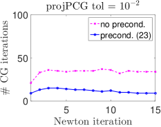
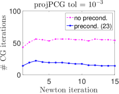
(d) Carbon Ash multi-frame

Figure 13: The effect of preconditioning by preconditioner defined in (39): number of projPCG iterations performed in each Newton iteration to achieve the desired tolerance. 5 % outliers.

The choice of projPCG tolerance is a difficult question, but from the average number of Newton iterations/projPCG iterations/fast Fourier transforms shown in Table 5, we observe that raising the tolerance does not considerably increase the number of Newton steps we need to perform here. Therefore larger tolerance, here $10^{-1}$, leads to a smaller total number of projPCG iterations. This is independent of the percentage of outliers. For each setting, the number of projPCG iterations is significantly smaller for the preconditioned version. This is not always the case for the total count of the fast Fourier transforms, since we need to perform 6 fft2/ifft2 in each iteration vs. 4 for the unpreconditioned iterations; see Table 1. For large scale problems, however, the computational complexity of fast Fourier transform, which is $\mathcal{O}(n\log n)$ is comparable to other operations performed in projPCG, such as the inner products, whose complexity is $\mathcal{O}(n)$, and therefore the number of projPCG iterations seems to be the more important indicator of efficiency of the preconditioner. Recall here that $n$ is the number of pixels in the image, so if we have a $256\times 256$ array of pixels, then $n=65535$.

Table 5: Average number of Newton iterations, projPCG iterations, and (inverse) 2D Fourier transforms for projPCG with and without preconditioning, and two tolerances on the relative size of the projPCG residual. Results are averaged over 10 independent realization of noise and outliers.

(a) projPCG tol = $10^{-1}$

average count: Newton/CG/fft2s
		% outliers
problem	precond	0%	2%	10%
Satellite single-frame	no	14/290/1383	14/274/1329	14/283/1374
	yes	15/161/1280	16/172/1362	14/158/1252
Satellite multi-frame	no	12/250/2398	12/216/2104	13/241/2364
	yes	12/107/1545	11/107/1535	12/103/1507
Carbon ash single-frame	no	11/190/939	10/179/891	11/184/915
	yes	10/71/641	11/72/654	13/82/753
Carbon ash multi-frame	no	14/221/2200	14/219/2179	16/254/2542
	yes	16/88/1510	15/85/1419	17/99/1654

(b) projPCG tol = $10^{-2}$

average count: Newton/CG/fft2s
		% outliers
problem	precond	0%	2%	10%
Satellite single-frame	no	13/536/2359	13/539/2373	14/641/2819
	yes	14/284/2001	15/302/2117	14/296/2091
Satellite multi-frame	no	11/457/4082	11/460/4130	12/499/4511
	yes	11/201/2536	11/197/2499	12/213/2747
Carbon ash single-frame	no	11/393/1754	11/432/1912	13/526/2315
	yes	10/121/934	11/129/1004	13/155/1201
Carbon ash multi-frame	no	13/426/3813	14/461/4127	16/498/4467
	yes	13/144/1954	14/150/2038	16/173/2359

6 Conclusion

We have presented an efficient approach to compute approximate solutions of a linear inverse problem that is contaminated with mixed Poisson–Gaussian noise, and when there are outliers in the measured data. We investigated the convexity properties of various robust regression functions and found that the Talwar function was the best option. We proposed a preconditioner, and illustrated that it was more effective than other standard preconditioning approaches on the types of problems studied in this paper. Moreover, we showed that a variant of the GCV method can perform well in estimating regularization parameters in robust regression. A detailed discussion of computational costs, and extensive numerical experiments illustrate the approach proposed in this paper is effective and efficient on image deblurring problems.

7 Acknowledgment

The authors would like to thank Lars Ruthotto for pointing them to the Projected PCG algorithm and providing them with a Matlab code. The first author would like to thank Emory University for the hospitality offered in academic year 2014-2015, when part of this work was completed.

References

- [1] J. M. Bardsley and J. Goldes. Regularization parameter selection methods for ill-posed Poisson maximum likelihood estimation. Inverse Prob., 25(9):095005, 2009.
- [2] J. M. Bardsley and C. R. Vogel. A nonnegatively constrained convex programming method for image reconstruction. SIAM J. Sci. Comput., 25(4):1326–1343, 2003/04.
- [3] M. Benzi and M. K. Ng. Preconditioned iterative methods for weighted Toeplitz least squares problems. SIAM J. Matrix Anal. Appl., 27(4):1106–1124, 2006.
- [4] S. Bonettini, R. Zanella, and L. Zanni. A scaled gradient projection method for constrained image deblurring. Inverse Prob., 25(1):015002, 2009.
- [5] B. Calef. Iteratively reweighted blind deconvolution. In 2013 IEEE International Conference on Image Processing, pages 1391–1393, Sept 2013.
- [6] D. Coleman, P. Holland, N. Kaden, V. Klema, and S. C. Peters. A system of subroutines for iteratively reweighted least squares computations. ACM Transactions on Mathematical Software (TOMS), 6(3):327–336, 1980.
- [7] H. S. Dollar. Constraint-style preconditioners for regularized saddle point problems. SIAM J. Matrix Anal. Appl., 29(2):672–684, 2007.
- [8] H. S. Dollar, N. I. M. Gould, W. H. A. Schilders, and A. J. Wathen. Using constraint preconditioners with regularized saddle-point problems. Computational Optimization and Applications, 36(2-3):249–270, 2007.
- [9] H. W. Engl, M. Hanke, and A. Neubauer. Regularization of inverse problems, volume 375 of Mathematics and its Applications. Kluwer Academic Publishers Group, Dordrecht, 2000.
- [10] J. A. Fessler and S. D. Booth. Conjugate-gradient preconditioning methods for shift-variant PET image reconstruction. IEEE Trans. Image Process., 8(5):688–699, 1999.
- [11] G. H. Golub, M. Heath, and G. Wahba. Generalized cross-validation as a method for choosing a good ridge parameter. Technometrics, 21(2):215–223, 1979.
- [12] P. Gravel, G. Beaudoin, and J. A. D. Guise. A method for modeling noise in medical images. IEEE Transactions on Medical Imaging, 23(10):1221–1232, Oct. 2004.
- [13] E. Haber. Computational methods in geophysical electromagnetics. Mathematics in Industry. SIAM, 2015.
- [14] M. Hanke, J. G. Nagy, and C. Vogel. Quasi-Newton approach to nonnegative image restorations. Linear Algebra Appl., 316(1-3):223–236, 2000. Conference Celebrating the 60th Birthday of Robert J. Plemmons (Winston-Salem, NC, 1999).
- [15] P. Hansen. Discrete inverse problems. Society for Industrial and Applied Mathematics, 2010.
- [16] P. C. Hansen, J. G. Nagy, and D. P. O’Leary. Deblurring images, volume 3 of Fundamentals of Algorithms. Society for Industrial and Applied Mathematics (SIAM), Philadelphia, PA, 2006. Matrices, spectra, and filtering.
- [17] P. C. Hansen, V. Pereyra, and G. Scherer. Least squares data fitting with applications. Johns Hopkins University Press, Baltimore, MD, 2013.
- [18] M. F. Hutchinson. A stochastic estimator of the trace of the influence matrix for Laplacian smoothing splines. Communications in Statistics – Simulation and Computation, 19(2):433–450, 1990.
- [19] C. Keller, N. I. M. Gould, and A. J. Wathen. Constraint preconditioning for indefinite linear systems. SIAM J. Matrix Anal. Appl., 21(4):1300–1317, 2000.
- [20] M. Kubínová and J. G. Nagy. Iteratively reweighted deconvolution and robust regression. In 16th AMOSTECH Conference Proceedings, 2015.
- [21] F. Luisier, T. Blu, and M. Unser. Image denoising in mixed Poisson-Gaussian noise. IEEE Transactions on Image Processing, 20(3):696–708, 2011.
- [22] M. Mäkitalo and A. Foi. Optimal inversion of the generalized Anscombe transformation for Poisson-Gaussian noise. IEEE Transactions on Image Processing, 22(1):91–103, 2013.
- [23] N. Mastronardi and D. P. O’Leary. Fast robust regression algorithms for problems with Toeplitz structure. Computational Statistics & Data Analysis, 52(2):1119–1131, 2008.
- [24] J. J. Moré and G. Toraldo. On the solution of large quadratic programming problems with bound constraints. SIAM J. Optim., 1(1):93–113, 1991.
- [25] V. A. Morozov. On the solution of functional equations by the method of regularization. Soviet mathematics – Doklady, 7:414–417, 1966.
- [26] J. L. Mueller and S. Siltanen. Linear and nonlinear inverse problems with practical applications, volume 10 of Computational Science & Engineering. Society for Industrial and Applied Mathematics (SIAM), Philadelphia, PA, 2012.
- [27] J. G. Nagy, K. Palmer, and L. Perrone. Iterative methods for image deblurring: a Matlab object-oriented approach. Numerical Algorithms, 36(1):73–93, 2004.
- [28] J. G. Nagy and Z. Strakoš. Enforcing nonnegativity in image reconstruction algorithms. In Proceedings of SPIE, volume 4121, pages 182–190, 2000.
- [29] D. P. O’Leary. Robust regression computation using iteratively reweighted least squares. SIAM J. Matrix Anal. Appl., 11(3):466–480, 1990. Sparse matrices (Gleneden Beach, OR, 1989).
- [30] D. L. Snyder, R. L. White, and A. M. Hammoud. Image recovery from data acquired with a charge-coupled-device camera. J. Opt. Soc. Am. A, 10(5):1014–1023, May 1993.
- [31] A. Staglianò, P. Boccacci, and M. Bertero. Analysis of an approximate model for Poisson data reconstruction and a related discrepancy principle. Inverse Prob., 27(12):125003, 2011.
- [32] C. R. Vogel. Computational methods for inverse problems, volume 23 of Frontiers in Applied Mathematics. Society for Industrial and Applied Mathematics (SIAM), Philadelphia, PA, 2002. With a foreword by H. T. Banks.