Synthesizing invariants by solving solvable loops

Abstract

When proving invariance properties of a program, we face two problems. The first problem is related to the necessity of proving tautologies of considered assertion language, whereas the second manifests in the need of finding sufficiently strong invariants. This paper focuses on the second problem and describes a new method for the automatic generation of loop invariants that handles polynomial and non deterministic assignments. This technique is based on the eigenvector generation for a given linear transformation and on the polynomial optimization problem, which we implemented in the open-source tool Pilat.

1 Introduction

Program verification relies on different mathematical foundations to provide effective results and proofs of the absence of errors. The problem is however undecidable for any Turing complete language, partly because of loops. This is one of the reasons why loop analysis is a highly studied topic in the field of verification.

Let us take for example linear filters, whose purpose is to apply a linear constraint to input signals. This particular kind of programs is difficult to analyze because of the non determinism induced by the unknown input signal. Here is an example of program inspired by linear filters:

⬇

x = non_det(-1,1);

y = non_det(-1,1);

while(x < 4) do

N = non_det(-0.1,0.1);

(x,y) = (0.68 * (x-y) + N, 0.68 * (x+y) + N);

done

We claim that loop invariants are a good solution in order to provide general information about such a loop. In this particular case, the loop admits the invariant $x^{2}+y^{2}\leqslant 14.9$ bounding the maximal value of $|x|$ and $|y|$ to $3.9$ : this is an infinite loop. More generally, if we can infer bounds for the value of the loop variables or for polynomial expressions of these variables we then are able to perform precise analyses such as reachability analyses.

We aim at facing two major problems of numeric invariant generation, namely the generation of polynomial relations between variables and the search of inductive spaces in which variables of a program belong to, in the context of simple (i.e. non-nested) loops composed of polynomial and non deterministic assignments. The relations we generate have the advantage to be completely independent from the initial state of the loop, making them fully generic, as opposed to full-program based techniques that start from a specific initial state. This work is an extension of the algorithm PILA introduced in [8], which generates polynomial equalities between variables manipulated by a simple deterministic loop. We show in this paper that a refined version of this algorithm can also produce inductive inequality invariants and tackle non-deterministic assignments as well as deterministic ones. Moreover, we add to this analysis an optimization algorithm enabling us to minimize the inductive set described by invariants of non deterministic loops.

Contributions.

The initial PILA approach [8] generates inductive invariants as equality relations (of the form $P(X)=0$ with $P$ a polynomial). We extend this method (Section 2) to generate new kinds of inductive invariants (of the form $P(X)\leqslant k$). It is mostly based on linear algebra and is applicable to C programs manipulating integers and floating point numbers ; to simplify we describe the method on a simple imperative language (Section 3). The two main results of this extension are the treatment of loops with deterministic (Section 4.1) and non-deterministic assignments (Section 4.2). In the latter case, we reduce the problem of generating invariants to the polynomial optimization problem. An algorithm for solving this problem is given. The proposed method in this paper is correct, fully implemented in Pilat and is currently part of the Frama-C suite [12] as an external open-source plug-in, available at [7]. We show its efficiency by applying it on several examples from related literature in section 6.

.

2 Overview

When synthesizing invariants, three ingredients are required :

1. what kind of invariants are computed ;

2. what will be their most useful shape ;

3. how strong they will be.

In abstract interpretation for example, we first choose the type of invariant that will be computed, i.e. the abstract domain, then a symbolic execution of properties of this domain will shape the initial state into an invariant that we will try to keep as strong as possible by applying appropriate widening and narrowing operators.

Deterministic case.

Let us first recall how PILA works on a simple example. Consider the loop of figure 1 for which we want to generate all invariants (polynomials $P$ such that $P(x,y)=0$) of degree $2$.

⬇

(x,y) = (non_det(-1,1),non_det(-1,1));

while(*) do

(x,y) = (0.68 * (x-y), 0.68 * (x+y));

done

Figure 1: Simple affine loop

Instead of starting with an initial state, which is not assumed to be known, we generate relations that are preserved by each step of the loop. Let $f$ be the loop transformation, (here $f(x,y)=(0.68*(x-y),0.68*(x+y))$. A linear application $\varphi$ is a semi-invariant if, given any valuation of the variables, it stays constant through one iteration of $f$. In other words, it must respect the following property:

If $\varphi(X)=0$ then $\varphi(f(X))=0$

In linear algebra, this is strictly equivalent to the following :

If $\varphi(X)=0$ then $f^{*}(\varphi)(X)=0$

where $f^{*}(\varphi)=\varphi\circ f$ is the dual application of $f$. If there exists a scalar $\lambda$ such that $f^{*}(\varphi)=\lambda.\varphi$ (i.e. $\varphi$ an eigenvector of $f^{*}$ associated to the eigenvalue $\lambda$) the criterion becomes obviously true, thus $\varphi$ is a semi-invariant.

By enhancing the loop expressiveness with new variables representing the value of the monomials of variables used in the loop, namely $x_{2}$ for $x^{2}$, $y_{2}$ for $y^{2}$ and $xy$ for $x*y$, we are also able to generate polynomial relations. Let us take for instance $x_{2}$. As the new value of $x$ is $0.68.(x-y)$, the new value of $x^{2}$ is $0.68^{2}.(x^{2}-2.x.y+y^{2})$. $x_{2}$ can then be expressed as a linear application of $x_{2}$, $xy$ and $y_{2}$. More generally, any monomial of variables of the loop in figure 1 evolves linearly along the execution of the enhanced loop. A linear invariant generation technique for linear loops can generate polynomial invariants by using the newly introduced variables.

We have shown in [8] that the eigenvectors of $f^{*}$ are exactly the set of such invariants bound to the transformation $f$ but we only investigated precisely what happened for the eigenspace associated to $1$, which returned affine invariants. When the associated eigenvalue was not $1$ we provided some methods in order to infer stronger invariants such as invariant simplification and removal of irrational invariants, but the resulting relations were still too weak. In the example of figure 1, the associated eigenvalue of the only invariant $x^{2}+y^{2}$ is $0.9248$. We can conclude that $x^{2}+y^{2}=0$ is inductive but if it does not respect the initial state, this is not an invariant.

The key idea of this paper is to consider not only equalities, but also inequalities. If the left eigenvector $\varphi$ is associated to an eigenvalue $\lambda$ such that $0<\lambda\leqslant 1$ then $\lambda.\varphi(X)$ will necessarily be smaller than $\varphi(X)$. Thus

If $\varphi(X)\leqslant k$ then $f^{*}(\varphi)(X)\leqslant k$

is true, and $\varphi(X)\leqslant k$ is inductive. In our example, the relation $x^{2}+y^{2}\leqslant k$ is inductive, and contrarily to $x^{2}+y^{2}=0$ it can be made an invariant even if the initial values of $x$ and $y$ are not $0$: we just have to choose $k=x_{init}^{2}+y_{init}^{2}$.

Non deterministic case.

The same reasoning can be applied to treat non deterministic values in assignments. By setting the non deterministic values to a random value, e.g. $0$, we are left to find inductive inequality relations, which can be easily performed as we just saw. In the deterministic case, generated formulas are inductive because the set of possible values for $x$ and $y$ that respects the formula gets bigger by applying the loop transformation once. Adding the non deterministic noise may lead to non inductive formulas. A solution consists in finding upper and lower bounds for this noise and check if the set obtained in deterministic case stays stable under this new transformation. If this is not the case, we must consider a weaker invariant.

3 Setting

Mathematical background.

Given a field $\mathbb{K}$ with a total ordering $\leqslant$, $\mathbb{K}^{n}$ is the vector space of dimension $n$. Elements of $\mathbb{K}^{n}$ are denoted $x=(x_{1},...,x_{n})^{t}$ a column vector. The variables vector of an application $f$ is denoted $X$. $\mathcal{M}_{n}(\mathbb{K})$ is the set of matrices of size $n*n$ and $\mathbb{K}[X]$ is the set of polynomials with coefficients in $\mathbb{K}$. We note $\overline{\mathbb{K}}$ the algebraic closure of $\mathbb{K}$, $\overline{\mathbb{K}}=\{x.\exists P\in\mathbb{K}[X],P(x)=0\}$. We will use $\left<.,.\right>$ the linear algebra standard notation, $\left<u,v\right>=u^{t}.v$, with . the standard dot product. The dual of a linear application $f$ associated to the matrix $A$ will be denoted $f^{*}$ and associated to the matrix $A^{t}$. The kernel of a matrix $A\in\mathcal{M}_{n}(\mathbb{K})$, denoted $\ker(A)$, is the vectorial space defined as $\ker(A)=\left\{x\in\mathbb{K}^{n},Ax=0\right\}$. Every matrix of $\mathcal{M}_{n}(\mathbb{K})$ admits a finite set of eigenvalues $\lambda\in\overline{\mathbb{K}}$ and their associated eigenspaces $E_{\lambda}$, defined as $E_{\lambda}=\ker(A-\lambda Id)$, where $Id$ is the identity matrix and $E_{\lambda}\neq\{0\}$. Similarly, every matrix $A$ admits left-eigenspaces, i.e. eigenspaces of $A^{t}$. We denote $|.|:\overline{\mathbb{K}}\rightarrow\mathbb{K}$ the modulus of an algebraic number and $\lVert.\rVert:\mathbb{K}^{n}\rightarrow\mathbb{K}$ the usual euclidean norm of a vector. The limit of a multivariate function $f:\mathbb{K}^{n}\rightarrow\mathbb{K}$ for $\lVert X\rVert\rightarrow l$ is defined by the maximal value of $f(X)$ with $\lVert X\rVert$ in the neighborhood of $l\in\mathbb{K}\cup\{+\infty\}$ and be denoted $\lim\limits_{\lVert X\rVert\rightarrow l}f$.

Invariants.

A formula requires two canonical properties to be an invariant: it must be true at the beginning of the loop (initialization); it must be preserved afterwards. Similarly to [8], we define the inductive relation $\varphi$ by the following constraint:

Definition 1

Exact

$\varphi\in\mathbb{K}^{n}$ is an exact inductive invariant for an application $f$ iff

$$\forall X,|\left<\varphi,X\right>|=0\Rightarrow|\left<\varphi,f(X)\right>|=0$$ (1)

We add to this definition the concept of convergent and divergent inductive relation :

Definition 2

Convergence

$\varphi\in\mathbb{K}^{n}$ is a convergent inductive invariant for an application $f$ iff

$$\forall X,\forall k\in\mathbb{K},|\left<\varphi,X\right>|\leqslant k\Rightarrow|\left<\varphi,f(X)\right>|\leqslant k$$ (2)

Definition 3

Divergence

$\varphi\in\mathbb{K}^{n}$ is a divergent inductive invariant for an application $f$ iff

$$\forall X,\forall k\in\mathbb{K}|\left<\varphi,X\right>|\geqslant k\Rightarrow|\left<\varphi,f(X)\right>|\geqslant k$$ (3)

A vector $\varphi$ satisfying the inductive relation is called a semi-invariant in contrast with invariants that also verifies the initialization criterion, denoted $\left<\varphi,X_{init}\right>\leavevmode\nobreak\ \leqslant\leavevmode\nobreak\ k$ for convergent invariants and $\left<\varphi,X_{init}\right>\leavevmode\nobreak\ \geqslant\leavevmode\nobreak\ k$ for divergent invariants with $X_{init}$ the variables’ initial values. The exact semi-invariants set of a linear application $f$ is the union of all eigenspaces of $f^{*}$ as proven in [8]. Also, we define the solvability of a mapping as introduced in [20].

Definition 4

Let $g\in(\mathbb{K}[X])^{m}$ be a polynomial mapping. $g$ is solvable if there exists a partition of $X$ into sub-vectors of variables $x=w_{1}\uplus...\uplus w_{k}$ such that $\forall j.\leavevmode\nobreak\ 1\leqslant j\leqslant k$ we have

$$g_{w_{j}}(x)=M_{j}w_{j}^{t}+P_{j}(w_{1},...,w_{j-1},N)$$

with $P_{j}$ a polynomial and $N$ eventual non deterministic parameters.

Remark.

We proved in [8] that deterministic solvable assignments are linearizable, i.e. they can be replaced by equivalent linear applications. This allows us to consider linear mappings $X^{\prime}=A.X$ with $X$ a vector containing both variables and monomials of those variables to represent solvable assignments.

Programming model.

We use a basic programming language whose syntax is given in figure 2. $Var$ is the set of variables used by the program. Variables take their value in a field $\mathbb{K}$. A program state is then a partial mapping $Var\rightharpoonup\mathbb{K}$. Any given program only uses a finite number $n$ of variables, thus program states can be represented as vectors $X=(x_{1},...,x_{n})^{t}$. Finally, we assume that for all programs, there exists $x_{n+1}=\mathds{1}$ a constant variable always equal to $1$. This allows to represent any affine assignment by a matrix.

$i$ ::=		skip
		| $i;i$
		| $(x_{1},..,x_{n}):=(exp_{1},...,exp_{n})$
		| while $*$ do $i$ done

$exp$ ::=		$cst\in\mathbb{K}$
		| $x\in Var$
		| $exp+exp$
		| $exp*exp$
		| $non\_det(exp,exp)$

Figure 2: Code syntax

The expression $non\_det(exp_{1},exp_{2})$ returns a random value between the valuation of $exp_{1}$ and $exp_{2}$ when the program reaches this location. Multiple variables assignments occur simultaneously within a single instruction. We say an assignment is affine (resp. solvable) when its right values is an affine (resp. solvable) combination. Also, we say that an instruction is non-deterministic when it is an assignment in which the right value contains the expression $non\_det$.

4 Convergent and divergent linear applications

4.1 Deterministic assignments

Being an inductive invariant requires for a formula $F$ to be true after an iteration of the loop under the hypothesis that $F$ holds before the iteration. The left eigenspace of a linear transformation (i.e. the eigenspace of the transformation dual) is exactly its set of exact invariants as defined in definition 1.

Convergence.

By linear algebra

$$|\left<\varphi,X\right>|\leavevmode\nobreak\ \leqslant k\Rightarrow|\left<f^{*}(\varphi),X\right>|\leqslant k$$ (4)

is strictly equivalent to the definition 2 of convergent semi-invariants. $|\left<\varphi,X\right>|\leqslant k$ represent what we call a domain described by $\varphi$, i.e. a polynomial relation. The previous constraint specify that the domain described by $\varphi$ is stable by $f$.

The loop in figure 1 admits the invariant $x^{2}+y^{2}\leqslant 2$, a domain described by $\varphi=(0,0,0,1,0,1)^{t}$ in the base $(\mathds{1},x,xy,x_{2},y,y_{2})$ where $x_{2}$ represents $x^{2}$, $xy$ represents $x*y$ and $y_{2}$ represents $y^{2}$. We can check with the PILA algorithm that $\varphi$ is an exact semi-invariant of the loop as it is a left eigenvector of the transformation performed by the loop. As such, it generates a vectorial space of exact semi-invariants $I=\{k.(x^{2}+y^{2})=0\leavevmode\nobreak\ |,k\in\mathbb{K}\}$, which is a very poor result as $x^{2}+y^{2}$ is constant only if it starts at $0$ (else, $k=0$ and we don’t know anything about $x^{2}+y^{2}$). We focus now on the eigenvalue associated to $\varphi$ on $f^{*}$, which is $0.9248$. Thus, we can replace $|\left<f^{*}(\varphi),X\right>|$ by $|\lambda|.|\left<\varphi,X\right>|$ in (4), which returns :

$$|\left<\varphi,X\right>|\leqslant k\Rightarrow|\lambda|.|\left<\varphi,X\right>|\leqslant k$$

As $|\lambda|<1$, the vector $\varphi$ satisfies the equation, thus $\varphi$ is a convergent semi-invariant. Knowing the maximal initial value of $x^{2}+y^{2}$ allows to determine the value of $k$, which is $2$. More generally, we have :

Property 1

$\varphi$ is a convergent semi-invariant $\Leftrightarrow\exists\lambda,|\lambda|\leqslant 1,f^{*}(\varphi)=\lambda.\varphi$

Proof

If $|\lambda|\leqslant 1$, then $\varphi$ is a convergent semi-invariant (see introduction of section 4.1). We will prove the following lemma:

Lemma 1

$\left(\forall k,|\left<\varphi,X\right>|\leqslant k\Rightarrow|\left<\varphi,f(X)\right>|\leqslant k\right)\Rightarrow f^{*}(\varphi)=\lambda.\varphi$

Proof

With $k=0$, we end up with the exact semi-invariant equation (1), whose solutions are eigenvectors of $f^{*}$. $\square$

As the exact semi-invariants set of $f$ is the union of the eigenspaces of $f^{*}$, we can deduce that this set is a superset of all the relations satisfying (2). Moreover by the lemma 2, we have

$$(|\left<\varphi,X\right>|\leqslant k\Rightarrow|\left<\varphi,f(X)\right>|\leqslant k)\Rightarrow(|<\varphi,X>|\leqslant k\Rightarrow|\lambda|.|<\varphi,X>|\leqslant k)$$

For $k=|<\varphi,X>|$ it is true if and only if $|\lambda|\leqslant 1$. $\square$

Divergence.

The same reasoning applies for the generation of divergent invariants. For example, an eigenvalue $\lambda$ such that $|\lambda|>1$ associated to a semi-invariant $\varphi$ implies that $|\left<\varphi,X\right>|\geqslant k$ is an inductive invariant. Thus, we also have

Property 2

$\exists\lambda,|\lambda|\geqslant 1,f^{*}(\varphi)=\lambda.\varphi\Rightarrow\varphi$ is a divergent semi-invariant

Proof

If there exists $\lambda$ such that $f^{*}(\varphi)=\lambda.\varphi$, then we have that

$$|<\varphi,X>|\leavevmode\nobreak\ \geqslant\leavevmode\nobreak\ k\Rightarrow|<\varphi,f(X)>|\leavevmode\nobreak\ \geqslant\leavevmode\nobreak\ k$$

is equivalent to

$$|<\varphi,X>|\leavevmode\nobreak\ \geqslant\leavevmode\nobreak\ k\Rightarrow|\lambda|.|<\varphi,X>|\leavevmode\nobreak\ \geqslant\leavevmode\nobreak\ k$$

If we also have that $|\lambda|>1$, then the previous equation is true. $\square$

Note that this is only an implication this time. For example, the transformation $f(x,\mathds{1})=(x+\mathds{1},\mathds{1})$ admits $x\geqslant x_{init}$ as a divergent invariant but the only left eigenvector of $f$ is $(0,1)$, which correspond to the invariant "$\mathds{1}$ is constant". Moreover, not all invariants of the form $P(X)\leqslant k$ are generated : the loop with the only assignment $x=x-1$ admits the (non-convergent) invariant $x\leqslant x_{init}$. This invariant does not enter the scope of our setting as $|x|\leqslant x_{init}$ is false for $2x_{init}+1$ iterations of $x=x-1$.

4.2 Non-deterministic assignments

Some programs depend on inputs given all along their execution, for example linear filters. More generally, an important part of program analysis consists in studying non-deterministic assignments. As an example let us consider the program in figure 3, a slightly modified version of the program in figure 1.

⬇

while (*) do

N = non_det(-0.1,0.1);

(x,y) = (0.68 * (x-y) + N, 0.68(x+y) + N);

done

Figure 3: Non deterministic variant of the example 1

Our previous reasoning is not applicable now because, due to the non-determinism of $N$, the loop is no longer a linear mapping.

Idea.

Intuitively, we will represent this loop by a matrix parametrized by $N$. For that purpose we use the concept of abstract application introduced in [10].

Definition 5

Let $I\subset\mathbb{K}$. An abstract linear application $f:\mathbb{I}^{q}\mapsto\mathcal{M}_{n}(\mathbb{K})$ is an application associating a $q-\mathit{tuple}(N_{1},...,N_{q})\in I^{q}$ to a matrix. We will call the $\mathit{tuple}$ the parameter of its image matrix by $f$, and $f^{*}$ the dual application of $f$ (i.e. the application such that $f^{*}(N)=(f(N))^{T}$). The expression of the parametrized matrix with respect to an abstract linear application will be called the abstract matrix.

In our setting, the parameters are the non-deterministic values. For example, the previous loop can be represented by the abstract matrix $M_{N}$ :

$$\left(\begin{array}[]{cccccc}1&0&0&0&0&0\\ N&0.68&0&0&-0.68&0\\ N^{2}&1.36N&0&0.462&0&-0.462\\ N^{2}&1.36N&0.925&0.462&-1.36N&0.462\\ N&0.68&0&0&0.68&0\\ N^{2}&1.36N&0.925&0.462&1.36N&0.462\end{array}\right)$$

We have shown in section 4.1 that $M_{0}$ admits the invariant $e_{0}=(0,0,0,1,0,1)$ associated to the eigenvalue $\lambda_{0}=0.9248$. By decomposing $M_{N}$ as the sum of $M_{0}$ and $(M_{N}-M_{0})$, we also have $e_{0}.M_{N}=e_{0}.M_{0}+e_{0}.(M_{N}-M_{0})=\lambda_{0}.e_{0}+\delta_{0}^{N}$, where $\delta_{0}^{N}=e_{0}.(M_{N}-M_{0})=(N^{2},2.72N,0,0,0,0)$. As the eigenvalue $\lambda_{0}$ is smaller than $1$, we are looking for relations $\varphi$ such that :

$$\forall X,|\left<\varphi,X\right>|\leqslant k\Rightarrow|\left<M_{N}^{T}.\varphi,X\right>|\leqslant k$$

We will call $e_{0}$ a candidate invariant for $M_{N}$. For $e_{0}$ to be an proper invariant for this transformation, the following property must hold:

$$\forall X,|\left<e_{0},X\right>|\leqslant k\Rightarrow|\lambda_{0}\left<e_{0},X\right>+\left<\delta_{0}^{N},X\right>|\leqslant k$$ (5)

Multiplying $|\left<e_{0},X\right>|$ by $|\lambda_{0}|$ reduces its value. We need to make sure that adding $\left<\delta_{0}^{N},X\right>$ does not contradict the induction criterion by increasing the result over $k$.

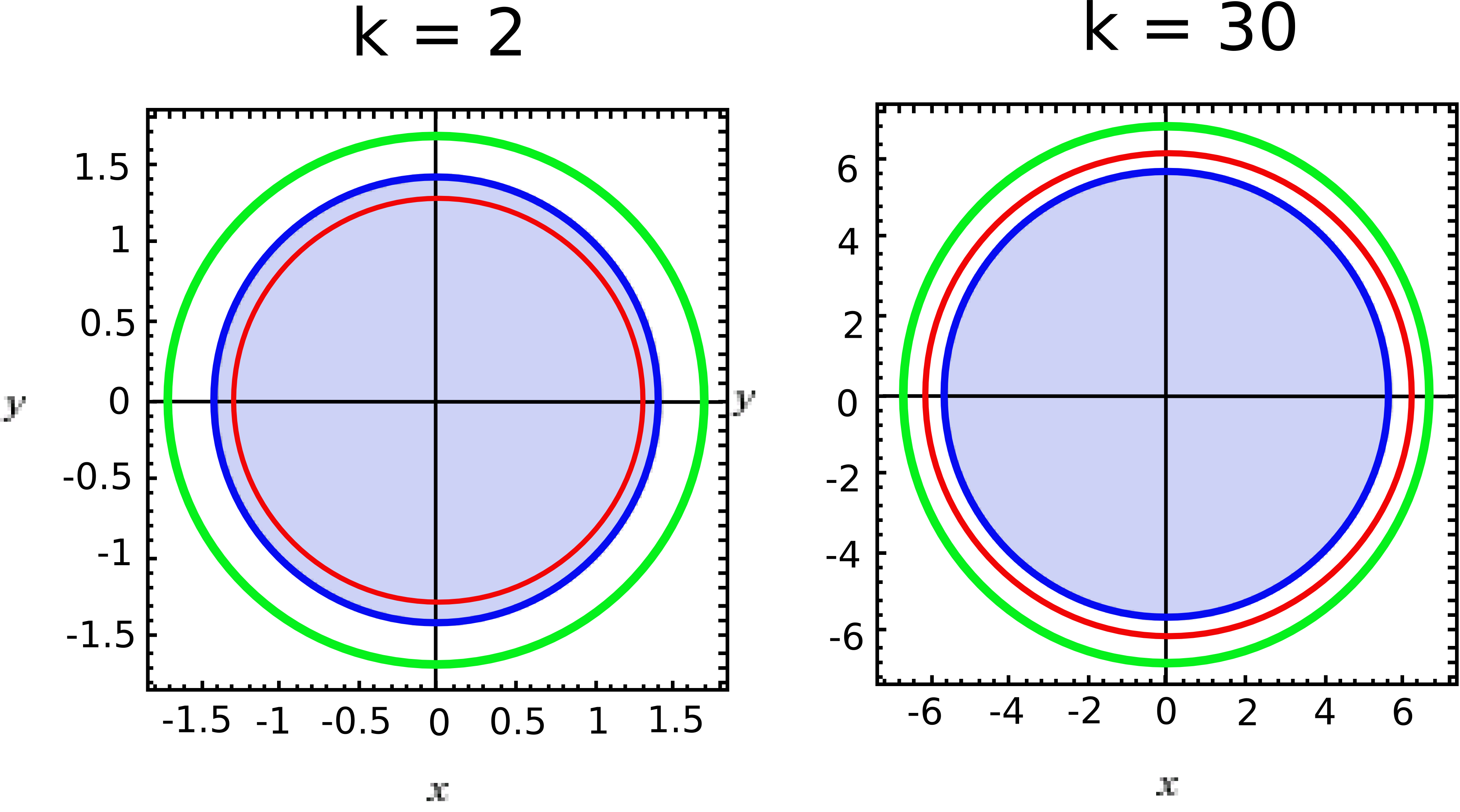
Figure 4: Representation of $x^{2}+y^{2}\leqslant k$ in blue, $|\lambda_{0}(x^{2}+y^{2})|\leqslant k$ in green and $|\lambda_{0}(x^{2}+y^{2})+max(\left<\delta_{0}^{N},X\right>)|\leqslant k$ in red.

We can see what happens on the figure 4. When multiplied by a $\lambda<1$, the value of $x^{2}+y^{2}$ becomes smaller, so the green circle $\lambda.(x^{2}+y^{2})\leqslant k$ is bigger than the blue one (more values of $x$ and $y$ fits the equation).

• In the first case $k$ is too small, adding $max(\left<\delta_{0}^{N},X\right>)$ reduces the green circle too much. Thus, the hypothesis that $(x,y)$ belongs to the blue circle does not imply it belongs to the red one: the candidate invariant is not inductive.

• In the second case, $max(\left<\delta_{0}^{N},X\right>)$ is too small to make the red back in the blue one: the candidate invariant is inductive.

The variables of the program depend on $k$, as does $\left<\delta_{0}^{N},X\right>$. If it increases faster than $|\lambda_{0}\left<e_{0},X\right>|$ when $k$ is increased, then no value of $k$ will make the candidate invariant inductive. In particular, if $\left<e_{0},X\right>$ is a polynomial $P$ of degree $d$, we need to be able to give an upper bound of $\left<\delta_{0}^{N},X\right>$ knowing that $|P(X)|<k$. If the degree of $\left<\delta_{0}^{N},X\right>$ is strictly smaller than $d$, then it will grow asymptotically slower than $|P(X)|$, thus for a big enough $k$ the induction criterion is respected.

Property 3

$\forall X,|\left<e_{0},X\right>|\leqslant k\Rightarrow|\lambda_{0}\left<e_{0},X\right>+\left<\delta_{0}^{N},X\right>|\leqslant k$ (5) $\Leftrightarrow$

$$\forall X,|\left<e_{0},X\right>|\leqslant k\Rightarrow|\left<\delta_{0}^{N},X\right>|\leqslant(1-|\lambda_{0}|).k$$ (6)

We try to find a $k$ big enough for the set to be inductive. From the property 3 we know that :

$$|\left<\varphi,X\right>|\leqslant k\Rightarrow-(1-\lambda_{0}).k\leqslant\left<\delta_{0}^{N},X\right>\leqslant(1-\lambda_{0}).k$$

In our example, $\left<\delta_{0}^{N},X\right>=2.72*N*x+2*N^{2}$. The polynomial $x$ is of degree $1$ while $<e_{0},X>=x^{2}+y^{2}$ is of degree $2$. We need to find a $k$ such that

$$-0.0752*k\leqslant 2.72*N*x+2*N^{2}\leqslant 0.0752*k$$ (7)

Optimizing expressions.

We need to maximize and minimize $2.72*N*x+2*N^{2}$, knowing the following three constraints:

• $x^{2}+y^{2}\leqslant k$

• $N\leqslant 0.1$

• $-0.1\leqslant N$

Solving this problem is very close to solving a constrained polynomial optimization (CPO) problem, a widely studied topic [2]. CPO techniques provide ways to find values minimizing and maximizing expressions constrained with inequalities between variables. Our main issue is related to the parameter $k$ that must be known in order to use CPO directly. We will investigate in this article not how CPO works in detail, but how we can reduce the problem of finding an optimal $k$ to the CPO problem, which enables us to use any CPO algorithm.

Assuming we have a function min computing the minimum, if it exists, of an expression under polynomial constraints, we propose an algorithm that refines the value of $k$ in figure 5.

Data:  

$\lambda$ : float

$f$ : objective function

$p$ : polynomial constraint

non_det_c : non deterministic constraints

$N$ : int

Result: $k$ such that $\forall X,P(X)\leqslant k\Rightarrow f(X)\leqslant|(1-ev)|.k$

low_k = 0;

up_k = MAX_INT;

k = MAX_INT / 2;

i = 0;

while i<N do

       i = i+1;

       Q = (P(x) + k);

       min = min(f,[Q] + non_det_c);

       max = min(-1*f,[Q] + non_det_c);

       if min > (-1+ev) * k and max < (1-ev)*k then

             up_k = k;

            

      else

             low_k = k;

            

       end if

      k = (low_k + up_k) / 2;

      

end while

Figure 5: Dichotomy search of a $k$ satisfying the condition (7)

The idea is to find $k$ by dichotomy.

• If $k$ doesn’t satisfy the constraints, we try a bigger one.

• If we find a $k$ satisfying the two conditions over $k$, then it is a potential candidate. We can still try to refine it by searching for a $k$ slightly smaller.

We can improve this algorithm by guessing an upper value of $k$ instead of taking an arbitrary maximal value MAX_INT. For our example, we started at $k=50$ and found that $k=14.9$ respects all the constraints.

• $x^{2}+y^{2}\leqslant 14.9\Rightarrow|x|\leqslant 3.9$

• $|N|\leqslant 0.1$

Thus $|2.72*x*N+2*N^{2}|\leqslant 1.0808$, and $k*0.0752=1.12$.

Remark.

Note however that the existence of a $k$ satisfying (7) is not guaranteed. For example, the set $S=\{(x,y,N)|x^{2}+y^{2}\leqslant k\wedge-0.1\leqslant N\leqslant 0.1\}$ is a compact set for any value of $k$, which means that $x$, $y$ and $N$ have maximum and minimum values. This implies the existence of a lower and an upper bound for every expression composed with $x$, $y$ and $N$, but the value of those expressions may be always higher than $k$ such as for $x^{2}+y^{2}+1$ bounded by $k+1$.

Property 4

Let $P$ and $Q$ two polynomials and $M>0\in\mathbb{R}$.

If $\lim\limits_{\lVert X\rVert\rightarrow+\infty}|\frac{Q(X)}{P(X)}|<M$, then there exists $k\in\mathbb{R}$ such that for all $k^{\prime}\geqslant k$

$$|P(X)|\leqslant k^{\prime}\Rightarrow|Q(X)|\leqslant M.k^{\prime}$$

By taking $M=(1-\lambda_{0})$, this theorem gives us a sufficient condition to guarantee the convergence of the algorithm in figure 5. As we are dealing with two polynomials $P$ and $Q$, then if $P$ (the candidate invariant) has a higher degree than $Q$ (the objective function) in all its variables, the limit of $\frac{Q(X)}{P(X)}$ will be null which is enough to ensure the convergence of the method. In our example, with $X=(x,y)$, $P(X)=x^{2}+y^{2}$ and $Q(X,N)=10.N(x^{2}+y^{2}+1)$, with $|N|\leqslant 0.1$. Because $\lim\limits_{\lVert X\rVert\rightarrow+\infty}|\frac{Q(X,N)}{P(X)}|=10N$ is higher than $1$ for $N=0.1$, the optimization procedure may not produce a result by theorem 4. In our case $Q(X)=2,72.x.N+2.N^{2}$ is a polynomial of degree $1$ in $x$ and $0$ in $y$, thus $\lim\limits_{\lVert X\rVert\rightarrow+\infty}|\frac{Q(X,N)}{P(X)}|=0$ and the optimization will converge.

Initial state.

The knowledge of the initial state is not one of our hypotheses yet, but the previous theorem provides the necessary information we need to treat the case where the initial state is strictly higher than the minimal $k$ we found. The previous theorem tells us that there exists a $K$ such that for all $K^{\prime}\geqslant K$, $K^{\prime}$ is a solution to the optimization problem. Our optimization algorithm is searching for a value of $k$ for which the set is inductive, though, and this solution may be only local : there may be a $k^{\prime}>k$ which is not a solution of the optimization procedure. If the value of $P(X_{init})$ is strictly higher than $k$, there are two possibilities :

• it satisfies the objective (7) and this is a right solution (optimization is then not necessary as $k=P(X_{init})$ is correct);

• it doesn’t satisfy the objective and we have to find a $k$ higher than $P(X_{init})$ satisfying it.

In both cases, we can enhance the optimization algorithm by first testing the objective (7) with $k=P(X_{init})$. If it does not respect the objective, then starting the dichotomy with $low\_k=P(X_{init})$ will return a solution (guaranteed by the theorem 4) strictly higher than $P(X_{init})$.

4.3 Rounding error.

When dealing with real life programs, performing floating point arithmetic generates rounding error. As for an input signal abstracted by a non deterministic value, we can add to every computation that may lead to a rounding error a non deterministic value whose bounds are determined by the variables types and values.

Addition.

Addition over two floating-point values lose some properties like associativity. For example, $(2^{64}-2^{64})+2^{-64}$ will be strictly equal to $2^{-64}$ but $2^{64}+(-2^{64}+2^{-64})$ will be equal to $0$. To deal with addition, we can consider the highest possible error between a real value and its floating point representation, a.k.a. the machine epsilon. It is completely dependent of the C type used : for float (single precision) it corresponds to $2^{-23}$ ; for double (double precision) it is $2^{-52}$. More generally, let $x$ and $y$ be two reals, with $\tilde{x}$ and $\tilde{y}$ their respective C representation. The IEEE standard model says that an operation on floating point numbers must be equivalent to an operation on the reals, and then round the result to one of the nearest floating point number. In this case, the relative error $|(\tilde{x}+\tilde{y})-(x+y)|=(x+y)*\varepsilon$ where $\varepsilon$ is the highest machine epsilon between the machine epsilon of the type of $x$, $y$ and $(x+y)$. The error is relative to the value of $x$ and $y$. This is not a problem, as we authorize in our setting non deterministic calls with expressions as argument.

Multiplication.

A similar approximation happen during a multiplication of two floating point values. The relative error $|(\tilde{x}*\tilde{y})-(x*y)|=x*y*\varepsilon$ Thus for every multiplication, we can add a non deterministic value between $-x*y*\varepsilon$ and $x*y*\varepsilon$.

With these considerations, we are able to provide precise bounds for rounding error for every operation performed in the loop.

Remark.

Note that we also can deal with value casting. For example, when a cast from a floating point value to a integer is performed, the maximal error is bounded by $1$ which can be abstracted in our setting by a non deterministic assignment.

5 Related work

There exist mainly two kinds of polynomial invariants: equality relations between variables, representing precise relations, and inequality relations, providing bounds over the different values of the variables. After the results of Karr in [11, 17] on the complete search of affine equality relations between variables of an affine program, Müller-Olm and Seidl [18] have proposed an inter-procedural method for computing polynomial equalities of bounded degree as invariants. For linear programs, Farkas’ lemma can be used to encode the invariance condition [4] under non linear constraints. Similarly, for polynomial programs, Gröbner bases have been shown to be an effective way to compute the exact relation set of minimal polynomial loop invariants composed of solvable assignments by computing the intersection of polynomial ideals [20, 19]. Even if this algorithm is known to be EXP-TIME complete in the degree of the invariant searched, high degree invariant is very rare for common loops and the tool Aligator [13], inspired from this technique for P-solvable loops[15, 14], is very efficient for low degree loops. Finally, [3] presents a technique that avoids the combination problem by using abstract interpretation to generate abstract invariants. This technique is implemented in the tool Fastind. The main issue is the completion loss: some invariants are missed and a maximal degree must be provided.

Synthesis of inequality invariants has become a growing field [16, 22], for example in linear filters analysis and automatic verification in general as it provides good knowledge of the variables bounds when computing floating point operations. Abstract interpretation [6] with widening operators allows good approximation of loops with the desired format. A recent work [9] mixes abstract interpretation and loop acceleration (i.e. the precise computation of the transitive closure of a loop) to extend the framework and obtain precise upper and lower bounds on variables in the polyhedron domain. Very precise and computing non-trivial relations for complex loops and conditions, it has the drawback to be applicable to a very restricted type of transformations (linear transformation with eigenvalues $\lambda$ such that $|\lambda|=0$ or $1$). We see this technique as complementary to ours as it generates invariants we do not find (such as $k\leqslant k_{init}$ for loop counters) and conversely. In order to treat non-deterministic loops, [16] refines as precisely as possible the set of reachable states for linear filters, harmonic oscillators and similar loops manipulating floating point numbers using a very specific abstract domain.

The PILA technique benefits from both of these domains as it is based on the synthesis of precise relations over the variables of the program [8] and avoids using abstract interpretation so that invariants have no predefined shape. As some of those relations are convergent(i.e. their valuation is reduced by every step of the loop) we can also deal with inequalities relations, and we provide a way to deal with non determinism with a technique inspired by policy iteration [5].

6 Application and results

The plug-in Pilat, written in OCaml as a Frama-C plug-in (compatible with the latest stable release, Aluminium) and originally generating exact relations for deterministic C loops, has been extended with convergent invariant generation and non deterministic loop treatment for simple C loops. It implements our main algorithm of invariant generation in addition to the optimization algorithm of figure 5, and generates invariants as ACSL [1] annotations, making them readily understandable by other Frama-C plugins. The tool is available at [7].

⬇

int simple_filter(int s0, int s1){

float r;

while (1) {

r = 1.5*s0 - 0.7*s1 + [-0.1,0.1]

s1 = s0;

s0 = r;

}

}

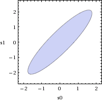
Figure 6: Generation of one of the smallest polynomial invariant of degree 2 for a linear filter [16, 24]

Let us now detail the work performed by Pilat over the example of figure 6 (taken from [16]). First, our tool generates the shape of the invariant, i.e. the polynomial $P$ such that $|P(X)|\leqslant k$ is inductive for a certain $k$ of the loop by setting the non deterministic choice to $0$. Here, the polynomial generated by Pilat is $P(s_{0},s_{1})=1.42857*s_{0}^{2}-2.14285*s_{0}*s_{1}+s_{1}^{2}$ with the eigenvalue $\lambda=0.7$. Adding the noise to the matrix returns the noise polynomial $Q(s_{0},s_{1},N)=2*N*s_{1}-2.142*N*s_{0}-1.428*N^{2}$ which has a lower degree than $P$ for a fixed $N$. Thus, we have that $\lim\limits_{\lVert(s0,s1)\rVert\rightarrow+\infty}\frac{Q(s0,s1,N)}{P(s0,s1)}=0<1-\lambda$. The optimization procedure is now certain to converge, thus we minimize and maximize $Q(X,N)$ with the hypothesis $P(s0,s1)\leqslant k$.

By starting the procedure with $k=50$ (which is usually a good heuristic) and performing $10$ iterations the optimization procedure returns $k=0.87891$, thus $1.42857*s_{0}^{2}-2.14285*s_{0}s_{1}+s_{1}^{2}\leqslant 0.87891$ is an inductive invariant.

Let us now consider that the initial state of the loop is $(s_{0},s_{1})=(2,1)$. Then at the beginning of the loop, $1.42857*s_{0}^{2}-2.14285*s_{0}s_{1}+s_{1}^{2}=2.42858>0.87891$, which does not respect the invariant. In this case the procedure starts by testing the optimization criterion with $k=2.14285$. This choice of $k$ is correct. In conclusion, we know that $1.42857*s_{0}^{2}-2.14285*s_{0}s_{1}+s_{1}^{2}\leqslant 2.42858$ is an invariant of the loop.

More generally, we evaluated our method over the benchmark used in [21] for which we managed to find an invariant for every program containing no conditions. Though this benchmark has been built to test the effectiveness of a specific abstract domain, we managed to find similar results with a more general technique. Our results are given in table 1.

Name	Var	Degree	# invariants	Candidate generation	Optimization
				(in ms)	(in s)
Simple linear filter	2	2	1	1.5	1.3
Simple linear filter	2	4	5	21	18
Example 3	2	2	1	3	1.7
Linear filter	4	2	1	1.9	1.5
Lead-lag controller	2	2	5	2.8	11
Gaussian regulator	2	2	1	7	2.5
Controller	4	1	2	1	5
Controller	4	2	5	66	14
Low-pass filter	5	2	4	60	7
Example 1	2	2	1	3	–
Dampened oscillator	4	2	1	7	–
Harmonic oscillator	4	2	1	4	–

Table 1: Performance results with our implementation Pilat. Tests have been performed on a Dell Precision M4800 with 16GB RAM and 8 cores. The first part of the benchmark are non deterministic loops. The second part represents deterministic loops (no optimization necesary).

As ellipsoids are a suitable representation for those examples, we have choosen $2$ as the input degree of almost all our examples. The optimization script is based on Sage [23]. Note that the candidate generation is a lot faster than the optimization technique, mainly because of two reasons :

• computing min is time consumung for a big number of constraints;

• it is imprecise and its current implementation is incorrect (it outputs a lower approximation of the answer). We have to compute verifications in order to find a correct answer.

7 Conclusion

Invariant generation for non deterministic linear loop is known to be a difficult problem. We provide to this purpose a surprisingly fast technique generating inductuve relations as it mostly relies on linear algebra algorithms widely used in many fields of computer science. Also, the optimization procedure for the non determinism treatment returns strong results. These invariants will be used in the scope of Frama-C [12] as a help to static analyzers, weakest precondition calculators and model-checkers. We are now facing three majors issues that we intend to address in the future: the current optimization algorithm is assumed to have an exact min function. However, such function is both time consuming and imprecise. In addition, conditions are treated non deterministically, which reduces the strength of our results and limits the size of our benchmark to simple loops (linear filters with saturation are not included in our setting). Finally, the search of invariants for nested loops is a complex problem on which we are currently focusing.

8 Appendix

8.1 Domain and codomains

The following justifies the two properties of section 4.1

Domain

Property 1

$\varphi$ is a convergent semi-invariant $\Leftrightarrow\exists\lambda,|\lambda|\leqslant 1,f^{*}(\varphi)=\lambda.\varphi$

Proof

If $|\lambda|\leqslant 1$, then $\varphi$ is a convergent semi-invariant (see introduction of section 4.1). We will prove the following lemma:

Lemma 2

$\left(\forall k,|\left<\varphi,X\right>|\leqslant k\Rightarrow|\left<\varphi,f(X)\right>|\leqslant k\right)\Rightarrow f^{*}(\varphi)=\lambda.\varphi$

Proof

With $k=0$, we end up with the exact semi-invariant equation (1), whose solutions are eigenvectors of $f^{*}$. $\square$

As the exact semi-invariants set of $f$ is the union of the eigenspaces of $f^{*}$, we can deduce that this set is a superset of all the relations satisfying (2). Moreover by the lemma 2, we have

$$(|\left<\varphi,X\right>|\leqslant k\Rightarrow|\left<\varphi,f(X)\right>|\leqslant k)\Rightarrow(|<\varphi,X>|\leqslant k\Rightarrow|\lambda|.|<\varphi,X>|\leqslant k)$$

For $k=|<\varphi,X>|$ it is true if and only if $|\lambda|\leqslant 1$. $\square$

Codomain

Property 2

$\exists\lambda,|\lambda|\geqslant 1,f^{*}(\varphi)=\lambda.\varphi\Rightarrow\varphi$ is a divergent semi-invariant

Proof

If there exists $\lambda$ such that $f^{*}(\varphi)=\lambda.\varphi$, then we have that

$$|<\varphi,X>|\leavevmode\nobreak\ \geqslant\leavevmode\nobreak\ k\Rightarrow|<\varphi,f(X)>|\leavevmode\nobreak\ \geqslant\leavevmode\nobreak\ k$$

is equivalent to

$$|<\varphi,X>|\leavevmode\nobreak\ \geqslant\leavevmode\nobreak\ k\Rightarrow|\lambda|.|<\varphi,X>|\leavevmode\nobreak\ \geqslant\leavevmode\nobreak\ k$$

If we also have that $|\lambda|>1$, then the previous equation is true. $\square$

8.2 Non-deterministic stability

The following justifies the stability condition property in section 4.2

Property 3

$\forall X,|\left<e_{0},X\right>|\leqslant k\Rightarrow|\lambda_{0}\left<e_{0},X\right>+\left<\delta_{0}^{N},X\right>|\leqslant k$ (5) $\Leftrightarrow$

$$\forall X,|\left<e_{0},X\right>|\leqslant k\Rightarrow|\left<\delta_{0}^{N},X\right>|\leqslant(1-|\lambda_{0}|).k$$ (8)

Proof

Let’s focus on the right part of the implication (5) :

$$|\lambda_{0}\left<e_{0},X\right>+\left<\delta_{0}^{N},X\right>| \leqslant k$$

$$-k\leqslant \lambda_{0}\left<e_{0},X\right>+\left<\delta_{0}^{N},X\right> \leqslant k$$

Our hypothesis is $|\left<e_{0},X\right>|\leqslant k$, which is equivalent to $-k\leqslant\left<e_{0},X\right>\leqslant k$.

• $\Leftarrow$

  If $\left<\delta_{0}^{N},X\right>\leqslant(1-\lambda_{0}).k$, then $\left<\delta_{0}^{N},X\right>+\lambda_{0}.k\leqslant k$. As $\lambda_{0}.\left<e_{0},X\right>\leqslant\lambda_{0}.k$, we have $\lambda_{0}.\left<e_{0},X\right>+\left<\delta_{0}^{N},X\right>\leqslant\lambda_{0}k+\left<\delta_{0}^{N},X\right>\leqslant k$.

  Dually if $\left<\delta_{0}^{N},X\right>\geqslant(\lambda_{0}-1).k$, then $\left<\delta_{0}^{N},X\right>-\lambda_{0}.k\geqslant-k$. As $\lambda_{0}.\left<e_{0},X\right>\geqslant-\lambda_{0}.k$, we have $\lambda_{0}.\left<e_{0},X\right>+\left<\delta_{0}^{N},X\right>\geqslant\left<\delta_{0}^{N},X\right>-\lambda_{0}.k\geqslant-k$.

• $\Rightarrow$

  We will perform a reasoning by the absurd. If there exist a $X$ such that $\left<\delta_{0}^{N},X\right>=(1-\lambda_{0}).k+\varepsilon$ with $\varepsilon>0$, then $\lambda_{0}.\left<e_{0},X\right>+\left<\delta_{0}^{N},X\right>=\lambda_{0}.\left<e_{0},X\right>+k-\lambda_{0}.k+\varepsilon$. In the case where $\left<e_{0},X\right>=k$ (which fits our hypotheses), $\lambda_{0}.\left<e_{0},X\right>+\left<\delta_{0}^{N},X\right>=k+\varepsilon>k$.

  Dually, if there exist a $X$ such that $\left<\delta_{0}^{N},X\right>=(\lambda_{0}-1).k-\varepsilon$ with $\varepsilon>0$, then $\lambda_{0}.\left<e_{0},X\right>+\left<\delta_{0}^{N},X\right>=\lambda_{0}.\left<e_{0},X\right>-k+\lambda_{0}.k-\varepsilon$.

  In the case where $\left<e_{0},X\right>=-k$ (which also fits our hypotheses), $\lambda_{0}.\left<e_{0},X\right>+\left<\delta_{0}^{N},X\right>=-k-\varepsilon<-k$.

$\square$

8.3 Boundedness of polynomials

The following justifies the boundedness property of polynomials in section 4.2

Property 4

Let $P$ and $Q$ two polynomials and $M>0\in\mathbb{R}$.

If $\lim\limits_{\lVert X\rVert\rightarrow+\infty}|\frac{Q(X)}{P(X)}|<M$, then there exists $k\in\mathbb{R}$ such that for all $k^{\prime}\geqslant k$

$$|P(X)|\leqslant k^{\prime}\Rightarrow|Q(X)|\leqslant M.k^{\prime}$$

Proof

If $\lim\limits_{\lVert X\rVert\rightarrow+\infty}|\frac{Q(X)}{P(X)}|<N$, then there exists $X$ such that for all $X^{\prime}$ with $\lVert X\rVert\leqslant\lVert X^{\prime}\rVert$ $-N\leqslant\frac{Q(X)}{P(X)}\leqslant N$

Let’s now add the hypothesis $|P(X)|\leqslant k$.

$-N\leqslant\frac{Q(X)}{P(X)}\leqslant N\Rightarrow-N\leqslant\frac{Q(X)}{k}\leqslant N$

$\square$

References

- [1] P. Baudin, J.-C. Filliâtre, C. Marché, B. Monate, Y. Moy, and V. Prevosto. ACSL: ANSI C Specification Language, 2008.
- [2] D. P. Bertsekas. Constrained optimization and Lagrange multiplier methods. Academic press, 2014.
- [3] D. Cachera, T. Jensen, A. Jobin, and F. Kirchner. Inference of polynomial invariants for imperative programs: A farewell to gröbner bases. Science of Computer Programming, 93, 2014.
- [4] M. A. Colón, S. Sankaranarayanan, and H. B. Sipma. Linear Invariant Generation Using Non-linear Constraint Solving, pages 420–432. Springer Berlin Heidelberg, Berlin, Heidelberg, 2003.
- [5] A. Costan, S. Gaubert, E. Goubault, M. Martel, and S. Putot. A policy iteration algorithm for computing fixed points in static analysis of programs. In International Conference on Computer Aided Verification, pages 462–475. Springer, 2005.
- [6] P. Cousot and R. Cousot. Abstract interpretation: a unified lattice model for static analysis of programs by construction or approximation of fixpoints. In Proceedings of the 4th ACM SIGACT-SIGPLAN symposium on Principles of programming languages, pages 238–252. ACM, 1977.
- [7] S. de Oliveira. Pilat. Available at https://github.com/Stevendeo/Pilat.
- [8] S. de Oliveira, S. Bensalem, and V. Prevosto. Polynomial invariants by linear algebra. Technical Report 16-0065/SDO, CEA, 2016. available at http://steven-de-oliveira.perso.sfr.fr/content/publis/pilat_tech_report.pdf.
- [9] L. Gonnord and P. Schrammel. Abstract acceleration in linear relation analysis. Science of Computer Programming, 93:125–153, 2014.
- [10] B. Jeannet, P. Schrammel, and S. Sankaranarayanan. Abstract acceleration of general linear loops. ACM SIGPLAN Notices, 49(1):529–540, 2014.
- [11] M. Karr. Affine relationships among variables of a program. Acta Informatica, 6(2):133–151, 1976.
- [12] F. Kirchner, N. Kosmatov, V. Prevosto, J. Signoles, and B. Yakobowski. Frama-C: A software analysis perspective. Formal Aspects of Computing, 27(3), 2015.
- [13] L. Kovács. Aligator: A mathematica package for invariant generation (system description). In Automated Reasoning. Springer, 2008.
- [14] L. Kovács. Reasoning algebraically about P-solvable loops. In International Conference on Tools and Algorithms for the Construction and Analysis of Systems, pages 249–264. Springer, 2008.
- [15] L. Kovács. A complete invariant generation approach for P-solvable loops. In Perspectives of Systems Informatics. Springer, 2010.
- [16] A. Miné, J. Breck, and T. Reps. An algorithm inspired by constraint solvers to infer inductive invariants in numeric programs. Submitted for publication, 2015.
- [17] M. Müller-Olm and H. Seidl. A note on karr’s algorithm. In Automata, Languages and Programming, pages 1016–1028. Springer, 2004.
- [18] M. Müller-Olm and H. Seidl. Precise interprocedural analysis through linear algebra. In ACM SIGPLAN Notices, volume 39. ACM, 2004.
- [19] E. Rodríguez-Carbonell and D. Kapur. Automatic generation of polynomial invariants of bounded degree using abstract interpretation. Science of Computer Programming, 64(1):54–75, 2007.
- [20] E. Rodríguez-Carbonell and D. Kapur. Generating all polynomial invariants in simple loops. Journal of Symbolic Computation, 42(4), 2007.
- [21] P. Roux. Analyse statique de systèmes de contrôle commande: synthèse d’invariants non linéaires. PhD thesis, Toulouse, ISAE, 2013.
- [22] P. Roux, R. Jobredeaux, P.-L. Garoche, and É. Féron. A generic ellipsoid abstract domain for linear time invariant systems. In Proceedings of the 15th ACM international conference on Hybrid Systems: Computation and Control, pages 105–114. ACM, 2012.
- [23] W. Stein et al. Sage: Open source mathematical software. 7 December 2009, 2008.
- [24] Wolfram|Alpha. Polynomial invariant for the simple_filter function, http://www.wolframalpha.com/input/?i=(-2.14285714286*(s1*s0)%2B1.42857142857*(s0*s0))%2B1.*(s1*s1)+%3C%3D++0.87891.