Instability in Reaction-Superdiffusion Systems

Abstract

We study the effect of superdiffusion on the instability in reaction-diffusion systems. It is shown that reaction-superdiffusion systems close to a Turing instability are equivalent to a time-dependent Ginzburg-Landau model and the corresponding free energy is introduced. This generalized free energy which depends on the superdiffusion exponent governs the stability, dynamics and the fluctuations of reaction-superdiffusion systems near the Turing bifurcation. In addition, we show that for a general n-component reaction-superdiffusion system, a fractional complex Ginzburg-Landau equation emerges as the amplitude equation near a Hopf instability. Numerical simulations of this equation are carried out to illustrate the effect of superdiffusion on spatio-temporal patterns. Finally the effect of superdiffusion on the instability in Brusselator model, as a special case of reaction-diffusion systems, is studied. In general superdiffusion introduces a new parameter that changes the behavior of the system near the instability.

I Introduction

Self-organized phenomena are ubiquitous in nature specially in living systems. They occur in open systems out of equilibrium and they have attracted the attention of scientists in different fields of science. In the study of self-organized phenomena, reaction-diffusion systems are extensively used Nicolis ; Kerner ; Buceta ; Mimura . They are sets of coupled partial differential equations which include diffusion terms. Reaction-diffusion systems are useful in many fields such as biology Harrison ; Meinhardt ; Murray1 ; Murray2 ; Chaplain ; Sherratt1 ; Sherratt2 ; Gatenby ; Kondo ; Shin , ecology Holmes ; Skellam , neuroscience Liang , physics Astrov ; Arecchi ; Staliunas , chemistry Castets and geology Heureux . They have rich dynamics and can produce spatio-temporal patterns Walgraef ; Haken ; Murray3 ; Cross1 ; Cross2 ; Aranson including traveling waves, kinks, vortices, domain walls, solitons, as well as hexagonal and stripe patterns.

Reaction diffusion systems were first proposed by Alan Turing in the study of morphogenesis Turing . Actually, Turing noticed that adding a diffusion term to a reaction system can derive the system to instability and plays an important role in the formation of spatio-temporal patterns out of equilibrium. There are two possible kinds of instability called Turing and Hopf. In fact, in a reaction-diffusion system, a steady state can experience a transition to an oscillating or a patterned state via a Hopf or Turing instability, respectively Kuramoto . The characteristic feature of most of the studied reaction-diffusion systems is that the diffusion is normal. However, experimental evidences show that anomalous diffusion arises more frequently in nature Bouchaud ; Haus ; Metzler1 ; Metzler2 ; Sokolov . This fact motivated us to consider anomalous diffusion in reaction-diffusion systems in this article.

In a normal diffusion the mean square displacement of a typical particle of the system grows linearly with time, $\langle x^{2}(t)\rangle\propto t$. Anomalous diffusion, on the other hand, is a diffusion process that does not obey this linear relation. In the most cases they satisfy a power law scaling relation, $\langle x^{2}(t)\rangle\propto t^{\gamma}$, which is present in variety of different systems. $\gamma$ is called anomalous diffusion exponent and for $\gamma=1$ we obtain the case of normal diffusion. $1<\gamma<2$, $0<\gamma<1$ and $\gamma=2$ correspond to a Levy superdiffusion, a subdiffusion and a ballistic diffusion, respectively Metzler1 . Both types of anomalous diffusion processes play important roles in various phenomena Wachsmuth ; Weiss ; Drazer ; Amblard ; Carreras ; Hansen ; Solomon ; Manandhar ; Sancho ; Angelico ; Viswanathan2 ; Sims ; Scher . For instance, subdiffusion often occurs in gels (especially bio-gels Wachsmuth ; Weiss ), porous media Drazer , and polymers Amblard . Levy superdiffusion is typical of some processes in plasmas and turbulent flows Carreras ; Hansen ; Solomon , surface diffusion Manandhar ; Sancho ; Angelico , animals hunting (especially for ocean predators and birds) Viswanathan2 ; Sims and charge carrier transfer in semiconductors Scher .

Although different aspects of anomalous diffusion as well as the properties of reaction-diffusion processes have been extensively studied separately, reaction-diffusion systems characterized by anomalous diffusion have been the subject of a limited number of studies Zhang ; Golovin ; Gambino ; Gafiychuk ; Henry ; Henry2 ; Langlands ; Weiss2 ; Nec ; Tzou ; Tzou2 . Addressing this shortcoming on one hand and the importance of recognition and control of instability in far from equilibrium systems on the other hand motivated us to study the instability of reaction-diffusion systems in the presence of anomalous superdiffusion.

Turing pattern formation in the Brusselator model with superdiffusion has been studied in Golovin . The authors have focused on the pattern selection in the formation of hexagons and stripes and have compared the case of normal and superdiffusion. Turing pattern formation has also been investigated in a typical activator-inhibitor system Zhang with a reaction term that has been first used to describe the chlorite-iodine-molonic acid Dufiet . It was found that the wave vector of patterns changes with the superdiffusion exponent which leads to a different size for Turing patterns. Nonlinear dynamics of an activator-inhibitor system with superdiffusion near the Hopf instability has been studied in Nec . It was shown that a fractional complex Ginzburg-Landau equation (FCGLE) governs the amplitude of critical mode in the vicinity of Hopf instability for two-component reaction-superdiffusion systems. Apart from mentioned studies, spatio-temporal patterns near a codimension-2 Turing-Hopf point, where Turing and Hopf instability thresholds coincide, have been considered in Tzou for a one dimensional superdiffusive Brusselator model and the long-wave stability of these patterns has been analyzed in Tzou2 .

Instability in a reaction-diffusion system is an example of non-equilibrium phase transitions. On the other hand in the vicinity of critical points fluctuations play an important role and the systems exhibit universal behavior. This motivated us to study the behavior of reaction-superdiffusion systems at the onset of instabilities and investigate the spectrum of fluctuations in the presence of superdiffusion. As the main part of our study we will show that any reaction-superdiffusion system in the vicinity of a Turing instability is equivalent to a time-dependent Ginzburg-Landau model. We will introduce the corresponding free energy which depends on the superdiffusion exponent. This free energy governs the instability, dynamics and the fluctuations of the system. In addition in the case of Hopf instability we generalize the two-component system of Nec to a n-component reaction-superdiffusion system. Utilizing the reductive perturbation method Kuramoto we show that a fractional complex Ginzburg-Landau equation governs the amplitude of the critical mode for a general n-component system, too. The solutions of FCGLE in two dimensions display a very rich spectrum of dynamical behavior. So we present numerical simulation of FCGLE in two dimensions to illustrate the effect of superdiffusion on spatio-temporal patterns near the Hopf instability. Finally we apply these general instability considerations to the Brusselator model in the presence of superdiffusion. Brusselator is a typical example of a reaction-diffusion system and is one of the most common non-linear chemical systems Golovin ; Reichl ; Walgraef2 .

This paper is organized as follows. In section II we review how superdiffusion can be considered in reaction-diffusion systems using the powerful tool of fractional calculus. The behavior of the reaction-superdiffusion system close to the Hopf and Turing instabilities is respectively investigated in sections III and IV. In section V the general instability considerations of the previous sections are applied to the Brusselator model. Finally conclusions and discussions are presented in section VI.

II Brief overview of reaction-superdiffusion systems

In this section we are going to consider anomalous diffusion in a reaction-diffusion system. In the introduction we presented a microscopic definition for the anomalous diffusion while reaction-diffusion systems are differential equations governing macroscopic quantities. Therefore we have to first introduce a macroscopic representation for the anomalous diffusion. To do this one can start with the microscopic point of view and then obtain a macroscopic equation for the anomalous diffusion in the continuum limit.

Suppose a normal diffusion. From a microscopic point of view, a normal diffusion is described by random motion of a particle with equal length of steps and equal waiting times between successive steps. This is the Brownian motion that in the continuum limit leads to the differential equation governing the normal diffusion process Metzler1 . However, both waiting time between successive jumps and the length of the steps may not be equal and can be extracted from continuous probability distribution functions. This is called the continuous random walk (CTRW) model which is used to describe anomalous diffusion Metzler1 ; Metzler2 ; Sokolov . In the subdiffusion process, due to the particle sticking and trapping, the waiting time probability distribution function is a heavy tailed function while in the case of Levy superdiffusion the length of steps obey such a heavy tailed function. When a particle experiences Levy flight instead of a Brownian motion, large jumps occur more frequently than the case of Brownian motion. Using CTRW approach accompanied by considering the power-law distribution function

$$P(x)\propto|x|^{-(1+\alpha)},$$ (1)

for steps, results in the one dimensional fractional diffusion equation

$$\frac{\partial n}{\partial t}=D_{\alpha}\frac{\partial^{\alpha}n}{\partial x^{\alpha}},$$

in the continuum limit Metzler1 where $D_{\alpha}$ is the generalized diffusion coefficient. $\alpha$ is the fractional order of the derivative that relates to $\gamma$ via $\alpha=2/\gamma$ where $\gamma$ appeared in the previously mentioned microscopic equation for mean square displacement of a particle in anomalous diffusion, $\langle x^{2}(t)\rangle\propto t^{\gamma}$. $n$ is a typical concentration in the system and $\frac{\partial^{\alpha}}{\partial x^{\alpha}}$ is the Weyl fractional operator $(1<\alpha<2)$ that is defined as

$$\frac{\partial^{\alpha}n}{\partial x^{\alpha}}=-\frac{1}{2\cos(\pi\alpha/2)}(\partial_{+}^{\alpha}n+\partial_{-}^{\alpha}n),$$

$$\partial_{+}^{\alpha}n=\frac{1}{\Gamma(2-\alpha)}\frac{d^{2}}{dx^{2}}\int_{-\infty}^{x}\frac{n(q,t)}{(x-q)^{\alpha-1}}dq,$$

$$\partial_{-}^{\alpha}n=\frac{1}{\Gamma(2-\alpha)}\frac{d^{2}}{dx^{2}}\int^{\infty}_{x}\frac{n(q,t)}{(q-x)^{\alpha-1}}dq,$$

where $\Gamma$ stands for the Gamma function Metzler1 ; Zhang ; Golovin . In higher dimensions, $\frac{\partial^{\alpha}}{\partial x^{\alpha}}$ operator is replaced by $\nabla^{\alpha}$, defined by its action in Fourier space, $\mathcal{F}(\nabla^{\alpha}n)=-|{\bf k}|^{\alpha}\mathcal{F}(n)$. Note that $\alpha$ in the probability distribution of jumps, (1), equals the order of the fractional derivative. Another interpretation for the index $\alpha$ comes from considerations of fractals and self-similarity. The path of a Brownian particle in space traces out a random fractal of dimension two, while a Levy particle draws a fractal of dimension $\alpha$.

A general n-component reaction-diffusion system is described by the following differential equation Kuramoto

$$\frac{\partial{\bf X}}{\partial t}={\bf F}({\bf X};\mu)+\mathcal{D}\nabla^{2}{\bf X},$$

where ${\bf X}$ and ${\bf F}$ are $n$-dimensional real vectors, $\mu$ is the bifurcation parameter and $\mathcal{D}$ is a diagonal matrix of diffusion coefficients. Therefore according to our discussion in this section, a general n-component reaction-superdiffusion system can be given by

$$\frac{\partial{\bf X}}{\partial t}={\bf F}({\bf X};\mu)+\mathcal{D}_{\alpha}\nabla^{\alpha}{\bf X},$$ (2)

where $\mathcal{D}_{\alpha}$ is a diagonal matrix of generalized diffusion coefficients. The characteristic feature of a reaction-superdiffusion system is that the fractional derivative introduces a new parameter, $\alpha$, that changes the properties of the solution.

III Hopf instability in reaction-superdiffusion systems

In this section we will study the behavior of a reaction-superdiffusion system in the vicinity of a Hopf bifurcation. Consider the general differential equation (2) governing a reaction-superdiffusion system. As $\mu$ varies the system may move from a steady state to a time-periodic state (limit cycle) near a Hopf bifurcation. Close to criticality, we are left with a couple of relevant dynamical variables whose time scales are distinguishably slower than the other dynamical variables, so that the latter can be eliminated adiabatically using the rescaled spacetime coordinate. This technique is called reductive perturbation method. As a result, (2) is contracted to a very simple universal equation. Here, in subsection A, we show that, in the case of a Hopf bifurcation, it is a fractional complex Ginzburg-Landau equation. Then the numerical study of FCGLE is presented in subsection B.

III.1 Formal Approach

Let ${\bf X}_{0}(\mu)$ be the steady solution of (2), ${\bf F}({\bf X}_{0};\mu)=0$. Taylor series expansion of (2) about the steady state, ${\bf u}({\bf r},t)={\bf X}-{\bf X}_{0}$, leads to

$$\frac{\partial{\bf u}}{\partial t}=({\bf L}+\mathcal{D}_{\alpha}\nabla^{\alpha}){\bf u}+{\bf Muu}+{\bf Nuuu}+...,$$ (3)

where ${\bf L}$ is the Jacobian matrix whose $ij$th element is $L_{ij}=\partial F_{i}({\bf X}_{0})/\partial X_{j}$. ${\bf Muu}$ and ${\bf Nuuu}$ are nonlinear terms that denote vectors (summation convention is used)

$${\bf Muu}=\frac{1}{2}\frac{\partial^{2}{\bf F}({\bf X}_{0})}{\partial X_{j}\partial X_{k}}u_{j}u_{k},$$ (4)

$${\bf Nuuu}=\frac{1}{6}\frac{\partial^{3}{\bf F}({\bf X}_{0})}{\partial X_{j}\partial X_{k}\partial X_{l}}u_{j}u_{k}u_{l}.$$ (5)

Note that the expansion coefficients, which are symbolically expressed by ${\bf M},{\bf N},...$ generally depend on $\mu$ at least through ${\bf X}_{0}(\mu)$. Assume that up to $\mu_{c}=0$, ${\bf X}_{0}$ is stable against small perturbations, while it loses stability for $\mu>0$. For a while, let’s forget about the special degrees of freedom coming from the fractional derivative in (2). The stability of ${\bf X}_{0}$ depends on the configuration of eigenvalues $\lambda$ given by

$${\bf L}{\bf u}=\lambda{\bf u}.$$

A hypothetical configuration of eigenvalues is plotted in Fig. 1.

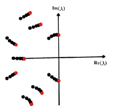
Figure 1: Schematic distribution of the eigenvalues. The eigenvalues of uniform and nonuniform modes have been shown in red and black, respectively Kuramoto .

Allowing, now, the diffusion term to be present causes the special modes to come into play. The linearized equation, in this case will be

$$\frac{\partial{\bf u}}{\partial t}=({\bf L}+\mathcal{D}_{\alpha}\nabla^{\alpha}){\bf u}.$$

Putting the normal mode solution of the form ${\bf u}={\bf V}_{\bf k}e^{\lambda t}e^{i{\bf k}.{\bf r}}$ in the above equation, one can easily find that in the presence of diffusion term a bunch of eigenvalues (corresponding to non-uniform modes) appear near each eigenvalue of ${\bf L}$ (Fig. 1). Also, the distance between two neighboring eigenvalues in the same branch is found to be of the order $\xi^{-\alpha}$ where $\xi\sim 1/k$ is a measure of the length of nonuniform modes and $k=|{\bf k}|$. This means that in each branch nonuniform modes with small wave vectors has eigenvalues close to the uniform mode. Therefore, these modes have comparable growth and decay rates with the uniform mode and affect the behavior of the system near the critical point ($\mu\rightarrow 0$). So, we have to take them into account.

Near the criticality, ${\bf L}$, ${\bf M}$, ${\bf N}$, eigenvectors and eigenvalues can be expanded in powers of $\mu$ as

$${\bf L}={\bf L^{(0)}}+\mu{\bf L^{(1)}}+\mu^{2}{\bf L^{(2)}}+...,$$

$${\bf M}={\bf M^{(0)}}+\mu{\bf M^{(1)}}+\mu^{2}{\bf M^{(2)}}+...,$$

$${\bf N}={\bf N^{(0)}}+\mu{\bf N^{(1)}}+\mu^{2}{\bf N^{(2)}}+...,$$

$${\bf u}=\mu^{\frac{1}{2}}{\bf u^{(1)}}+\mu{\bf u^{(2)}}+\mu^{\frac{3}{2}}{\bf u^{(3)}}+...,$$

$$\lambda=\lambda^{(0)}+\mu\lambda^{(1)}+\mu^{2}\lambda^{(2)}+...,$$

where $\lambda^{(0)}=\pm i\omega_{0}$ and $\lambda^{(i)}=\sigma_{i}+i\omega_{i}$. We must get inside the neighborhood of the critical mode and we do this by rescaling the space and time variables. Since $\lambda$ has real part of order $\mu$ and the characteristic time is equal to the inverse of the real part of $\lambda$, time is naturally rescaled according to

$$\tau=|\mu|t.$$

However, rescaling the space requires more details. In fact we should define a length scale for which nonuniform modes become important in the dynamics of the system. For this purpose, note that the characteristic time scale of critical modes is $\tau_{0}\sim\mu^{-1}$ Kuramoto . However, for the slowest nonuniform modes it roughly is $\tau_{\nu}\sim(\mu+\xi^{-\alpha})^{-1}$ where we have ignored $D_{\alpha}$ in the scaling argument. These two characteristic times are of the same order if $|\mu|\sim\xi^{-\alpha}$. Therefore, those nonuniform modes whose wavelengths are greater than $\xi>|\mu|^{-\frac{1}{\alpha}}$ play a role in the long time behavior of the system. This suggests us to introduce a scaled coordinate $s$ defined by

$$s=|\mu|^{\frac{1}{\alpha}}r=\varepsilon^{\frac{2}{\alpha}}r,$$

where $\varepsilon^{2}\chi\equiv\mu$ and $\chi=sgn(\mu)$. Based on the above discussion, ${\bf u}$ is regarded as a function of $t$, $\tau$, and $s$. This means that we are dealing with the long time, long wavelength modes in their natural variables $\tau$ and $s$, and reserving $t$ for the overall periodic motion (limit cycle). Also note that $\nabla\rightarrow\varepsilon^{2/\alpha}\nabla_{\bf s}$, so, $\nabla^{\alpha}\rightarrow\varepsilon^{2}\nabla^{\alpha}_{\bf s}$. Substitution of (III.1) into (3) and equating coefficients of different powers of $\varepsilon$, yields to a set of equations in the form of

$$(\frac{\partial}{\partial t}-{\bf L^{(0)}}){\bf u^{(\boldsymbol{\nu})}}={\bf B_{\boldsymbol{\nu}}},\;\;\;\nu=1,2,...,$$ (7)

where the first three $\bf B$’s are

$${\bf B_{1}}={\bf 0},$$

$${\bf B_{2}}={\bf M^{(0)}}{\bf u^{(1)}}{\bf u^{(1)}},$$

$${\bf B_{3}}=-(\frac{\partial}{\partial\tau}-\chi{\bf L^{(1)}}-\mathcal{D}_{\alpha}\nabla^{\alpha}_{\bf s}){\bf u^{(1)}}+2{\bf M^{(0)}u^{(1)}u^{(2)}}+{\bf N^{(0)}u^{(1)}u^{(1)}u^{(1)}}.$$

Note that the term with fractional derivative contributes to the coefficient of $\varepsilon^{3}$.

There is a solvability condition for the set of equations (7) Kuramoto , which for $\nu=1$ leads to

$${\bf u^{(1)}}(t,\tau,s)=W(\tau,s){\bf U_{R}}e^{i\omega_{0}t}+c.c,$$

where $c.c.$ stands for the complex conjugate, ${\bf U_{R}}$ is the right eigenvector of ${\bf L^{(0)}}$, and $W(\tau,s)$ is a complex amplitude to be determined. The right eigenvector and left eigenvector $({\bf U_{L}})$ are normalized in such a way that ${\bf U_{L}}{\bf U_{R}}=1$. The solvability condition for $\nu=2$ gives rise to an expression for ${\bf u^{(2)}}$

$${\bf u^{(2)}}={\bf V_{+}}W^{2}e^{2i\omega_{0}t}+{\bf V_{-}}\overline{W}^{2}e^{-2i\omega_{0}t}+{\bf V_{0}}|W|^{2},$$

where

$${\bf V_{+}}={\bf\overline{V}}_{-}=-({\bf L^{(0)}}-2i\omega_{0}{\bf I})^{-1}{\bf M^{(0)}U_{R}U_{R}},$$

$${\bf V_{0}}=-2{\bf L^{(0)}}^{-1}{\bf M^{(0)}U_{R}\overline{U}_{R}}.$$

The bar stands for complex conjugate, ${\bf I}$ is the identity matrix and the operator ${\bf M}$ can be read off from (4). Putting ${\bf u^{(1)}}$ and ${\bf u^{(2)}}$ into the solvability condition for $\nu=3$ results in the equation governing the amplitude $W$

$$\frac{\partial W}{\partial\tau}=\chi\lambda^{(1)}W+d\nabla^{\alpha}_{\bf s}W-g|W|^{2}W,$$ (8)

where $\lambda^{(1)}$, $d$ and $g$ are generally complex numbers that are given by

$$\lambda^{(1)} = {\bf U_{L}}{\bf L^{(1)}}{\bf U_{R}},$$ (9)

$$d = d_{r}+id_{i}={\bf U_{L}}\mathcal{D}_{\alpha}{\bf U_{R}},$$ (10)

$$g \equiv g_{r}+ig_{i}=4{\bf U_{L}M^{(0)}U_{R}}{\bf L^{(0)}}^{-1}{\bf M^{(0)}U_{R}\overline{U}_{R}}$$ (11)

$$+ 2{\bf U_{L}M^{(0)}\overline{U}_{R}}({\bf L^{(0)}}-2i\omega_{0}{\bf I})^{-1}{\bf M^{(0)}U_{R}U_{R}}-3{\bf U_{L}N^{(0)}U_{R}U_{R}\overline{U}_{R}}.$$ (12)

(8) is a fractional Ginzburg-Landau equation and has non-trivial oscillatory solutions, in the absence of diffusive term, provided that $g_{r}$ and $\chi$ have the same sign Kuramoto ; Moralesa . These solutions are stable in the case of $\chi>0$, supercritical Hopf bifurcation, and unstable for $\chi<0$, subcritical Hopf bifurcation. So the stability condition implies the simultaneous establishment of the conditions $g_{r}>0$ and $\chi>0$. We implicitly assume that these conditions are fulfilled here. With a redefinition as follows

$$r^{\prime}=({\sigma_{1}/d_{r}})^{1/\alpha}s,\;\;\;t^{\prime}=\sigma_{1}\tau,\;\;\;W^{\prime}=\sqrt{g_{r}/\sigma_{1}}e^{-i\omega_{1}\tau}W,$$

FCGLE above criticality can be written in a more convenient form (dropping the primes)

$$\frac{\partial W}{\partial t}=W+(1+ic_{1})\nabla^{\alpha}W-(1+ic_{2})|W|^{2}W,$$ (13)

where $c_{1}=d_{i}/d_{r}$ and $c_{2}=g_{i}/g_{r}$. It is obvious from (13) that superdiffusion can change the properties of the solution by changing the order of derivative as well as the parameter $c_{1}$.

To study (13) in more details, note that the first term of the r.h.s is related to the linear instability mechanism which leads to oscillations. The second term accounts for diffusion and dispersion while the third one is a cubic non-linear term. The competition between these three terms results in different regimes. There are two interesting limits for (13) which are worth mentioning. For $c_{1},c_{2}\rightarrow 0$, (13) reduces to a time-dependent fractional real Ginzburg-Landau equation (FRGLE) and as $c_{1},c_{2}\rightarrow\infty$, one obtains a fractional nonlinear Schrödinger equation.

Analytical and numerical solutions of FCGLE in one dimension and also some aspects of numerical simulations in two dimensions have been presented in Nec . Since the solutions of FCGLE in two dimensions display a very rich spectrum of dynamical behavior we were encouraged to present a comprehensive numerical study of these solutions in two dimensions in the next subsection. This enables us to observe the effect of fractional order, $\alpha$, on the spatio-temporal patterns.

III.2 Numerical Simulations

As was mentioned, FCGLE possesses a rich dynamics in two dimensions and such as its special case, CGLE Chate , has three different regimes. There are two kinds of disordered regimes called phase turbulence and defect turbulence, depending on whether they exhibit defects or not. In phase turbulence regime the amplitude of the field $W$ never reaches zero while this amplitude becomes zero at some points for defect (amplitude) turbulence regime. Apart from these two disordered regimes there are frozen states those in which $|W|$ is stationary in time. Cellular structures and spiral patterns can be observed in this regime.

As we saw in Eq. (13), superdiffusion changes both the order of spatial derivative and the parameter $c_{1}$. On the other hand, variation of any of the parameters in CGLE can affect the solutions Chate . Here we are interested in the effect of fractional derivative on the solutions of FCGLE, so we neglect the dependence of $c_{1}$ on $\alpha$.

For solving FCGLE we use a pseudospectral method to perform numerical computations in Fourier space. The numerical simulation is based on the method of exponential time differencing (ETD2) Cox . Small amplitude random initial data about $W=0$ and periodic boundary conditions are used.

We start with the values of $c_{1}$ and $c_{2}$ for which in the case of normal diffusion, CGLE leads to the frozen states (for instance see Fig. 2.a, 2.b) with cellular structures (Fig. 2.b). It is seen in Fig. 2.a, that there are no apparent spiral waves in the case of normal diffusion for the selected parameters. With the same parameters in the case of superdiffusion, as $\alpha$ decreases, cellular structures with larger size are formed and then with further decrease of $\alpha$, spiral waves emerge (Fig. 2.c). Fig. 2.f shows that as $\alpha$ becomes smaller, the domain walls (shock lines) almost melt and as can be seen in Fig. 2.e a mixed state appears in which some spirals live in a disordered sea. Finally the spiral patterns as well as the cellular structures disappear completely as one further reduces the value of $\alpha$. In this stage we obtain spatio-temporal patterns for which $|W|$ is not stationary in time and becomes zero at some points (Fig. 2.h). This is the fully developed defect turbulence regime according to its definition. Therefore, numerical simulations show that superdiffusion can create and annihilate spiral patterns and can make a transition from one regime to another. In fact the magnitude of diffusion and dispersion terms become larger in the presence of superdiffusion and the competition between the three terms in r.h.s of (13) changes in comparison with the case of normal diffusion and can even lead to the probable change of regimes.

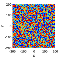
(a)

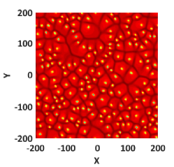
(b)

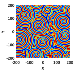
(c)

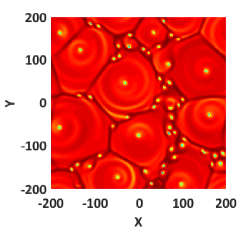
(d)

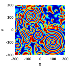
(e)

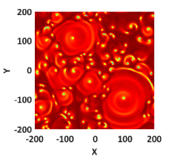
(f)

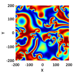
(g)

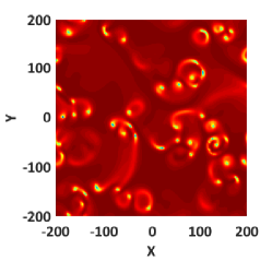
(h)

Figure 2: Snapshots of solutions of (13) for the parameters $c_{1}=0.55$, $c_{2}=-0.45$ and the system size $L=400$. Left panel, $Re(W)$, and right panel, $|W|$, with $\alpha=2$ for (a) and (b); $\alpha=1.46$ for (c) and (d); $\alpha=1.4$ for (e) and (f) and $\alpha=1.3$ for (g) and (h).

Numerical simulations indicate that in the defect turbulence regime, density of defects reduces gradually by the decrease of fractional order, $\alpha$. For instance in Fig. 3 the parameters are chosen in such way that we are in the defect turbulence regime of CGLE with a large density of defects (Fig. 3.a, 3.b) and it is seen that the density of defects decreases in the presence of superdiffusion (Fig. 3.c, 3.d).

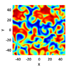
(a)

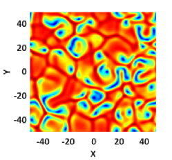
(b)

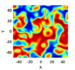
(c)

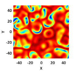
(d)

Figure 3: Defect turbulence regime: Snapshots of solutions of (13) for the parameters $c_{1}=1$, $c_{2}=-1.2$ and the system size $L=100$. Left panel, $Re(W)$, and right panel, $|W|$, with $\alpha=2$ for (a) and (b) and $\alpha=1.1$ for (c) and (d).

For the phase turbulence regime, as can be seen in Fig. 4 as an example, the amplitude of fluctuations increases in the superdiffusion case.

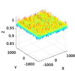
(a)

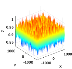
(b)

Figure 4: Phase turbulence regime: Snapshots of solutions of (13) for the parameters $c_{1}=2$, $c_{2}=-1$ and the system size $L=2500$. Plot of $|W|$ for (a) $\alpha=2$ and (b) $\alpha=1.1$.

After investigation of different regimes in FCGLE, we proceed by studying the interesting limit of this equation, $c_{1},c_{2}\rightarrow 0$, which is the time-dependent fractional real Ginzburg-Landau equation. Dynamics of this equation results in stationary patterns for both $Re(W)$ and $|W|$ (Fig. 5). For the case of normal diffusion, $\alpha=2$, FRGLE reduces to real Ginzburg-Landau equation (RGLE) which has been used to describe the spinodal decomposition in critical quench Petschek . Simulations of time-dependent RGLE results in domain patterns that can be seen in figures 5.a and 5.d. For the superdiffusion case, i.e. $\alpha\neq 2$, the domain patterns also form for the FRGLE but, as is clear from figures 5.b, 5.e, 5.c and 5.f, larger size domains appear as $\alpha$ decreases.

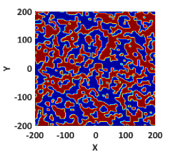
(a)

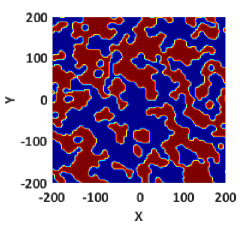
(b)

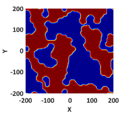
(c)

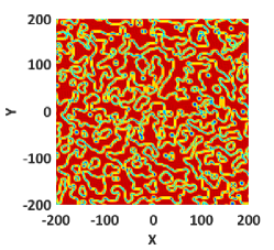
(d)

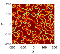
(e)

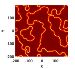
(f)

Figure 5: Snapshots of solutions of (13) for the parameters $c_{1}=c_{2}=0$ and the system size $L=400$. Upper panel, $Re(W)$, and lower panel, $|W|$, with $\alpha=2$ for (a) and (d); $\alpha=1.5$ for (b) and (e) and $\alpha=1.1$ for (c) and (f).

IV Turing instability in reaction-superdiffusion systems

In the previous section we studied the behavior of a reaction-superdiffusion system near a Hopf instability. In this section we are going to describe a two-component reaction-superdiffusion system in the vicinity of a Turing instability. In fact, a generalized thermodynamic potential, free energy, will be eventually presented which governs the stability, the dynamics and the fluctuations of reaction-superdiffusion systems near the Turing bifurcation. To reach this goal we include a local noise term in the linearized system of reaction-superdiffusion equations. Note that the reason for considering a two-component system in this section is that we want to present an analytic expression for the free energy.

Recall the general equation (2) for a n-component reaction-superdiffusion system. For a two-component system ${\bf X}({\bf r},t)$ and ${\bf F}({\bf X};\mu)$ are given by ${\bf X}({\bf r},t)=\left(\begin{array}[]{cc}X_{1}({\bf r},t)\\ X_{2}({\bf r},t)\end{array}\right)$ and ${\bf F}({\bf X};\mu)=\left(\begin{array}[]{cc}F_{1}(X_{1},X_{2};\mu)\\ F_{2}(X_{1},X_{2};\mu)\end{array}\right)$ and therefore (2) in the presence of noise is written as

$$\left\{\begin{array}[]{cc}\frac{\partial X_{1}}{\partial t}=D_{\alpha 1}\nabla^{\alpha}X_{1}+F_{1}(X_{1},X_{2};\mu)+\xi_{1}({\bf r},t)\\ \frac{\partial X_{2}}{\partial t}=D_{\alpha 2}\nabla^{\alpha}X_{2}+f_{2}(X_{1},X_{2};\mu)+\xi_{2}({\bf r},t)\end{array}\right.,$$ (14)

where $\xi_{1}$ and $\xi_{2}$ are noise terms that generally depend on $\bf r$ and $t$. This two-component reaction-superdiffusion system is known as activator-inhibitor system where $X_{1}$ and $X_{2}$ are activator and inhibitor, respectively. We consider the noise terms to be Gaussian white noises with the following properties

$$\langle\xi_{1}({\bf r},t)\rangle=\langle\xi_{2}({\bf r},t)\rangle=0,$$

$$\langle\xi_{1}({\bf r},t)\xi_{1}({\bf r^{\prime}},t^{\prime})\rangle=\langle\xi_{2}({\bf r},t)\xi_{2}({\bf r^{\prime}},t^{\prime})\rangle=2\zeta\delta^{d}({\bf r}-{\bf r^{\prime}})\delta(t-t^{\prime}),$$ (15)

$$\langle\xi_{1}({\bf r},t)\xi_{2}({\bf r^{\prime}},t^{\prime})\rangle=0.$$

Similar to the expansion in the section III, we expand (14) about the steady state, ${\bf u}({\bf r},t)={\bf X}-{\bf X}_{0}$, where for the two-component system ${\bf u}({\bf r},t)=\left(\begin{array}[]{cc}u_{1}({\bf r},t)\\ u_{2}({\bf r},t)\end{array}\right)$. By choosing the linear part of the expanded equations and transforming to Fourier space, the system of equations (14) takes the form

$$i\omega\left({{\begin{array}[]{cc}\tilde{u}_{1}({\bf k},\omega)\\ \tilde{u}_{2}({\bf k},\omega)\\ \end{array}}}\right)-\left({{\begin{array}[]{cc}L_{11}-D_{\alpha 1}k^{\alpha}&L_{12}\\ L_{21}&L_{22}-D_{\alpha 2}k^{\alpha}\\ \end{array}}}\right)\left({{\begin{array}[]{cc}\tilde{u}_{1}({\bf k},\omega)\\ \tilde{u}_{2}({\bf k},\omega)\\ \end{array}}}\right)=\left({{\begin{array}[]{cc}\tilde{\xi}_{1}({\bf k},\omega)\\ \tilde{\xi}_{2}({\bf k},\omega)\\ \end{array}}}\right),$$ (16)

where $L_{ij}$’s are the components of the Jacobian matrix. The $2\times 2$ matrix in (16)

$${\cal L}=\left({{\begin{array}[]{cc}L_{11}-D_{\alpha 1}k^{\alpha}&L_{12}\\ L_{21}&L_{22}-D_{\alpha 2}k^{\alpha}\\ \end{array}}}\right),$$

contains the information about the critical behavior of the system.

To proceed towards studying the system near the Turing instability we first need to find the eigenvalues and eigenvectors of $\cal L$ at the critical point as well as an analytic expression for its eigenvalues close to the critical point. Therefore in the subsection A we calculate these quantities first and find out how they vary in the presence of superdiffusion. Then we use them to study the behavior of the system in subsection B.

IV.1 The eigenvalue of the slow mode near the criticality

The eigenvalues of $\cal L$ can be derived from the characteristic equation

$$\lambda^{2}+g\lambda+h=0,$$ (17)

where

$$g=(D_{\alpha 1}+D_{\alpha 2})k^{\alpha}-L_{11}-L_{22},$$ (18)

$$h=(L_{11}-D_{\alpha 1}k^{\alpha})(L_{22}-D_{\alpha 2}k^{\alpha})-L_{12}L_{21}.$$ (19)

$g$ and $h$ are functions of $k^{\alpha}$ and through $L$’s they also depend on the bifurcation parameter $\mu$. Conventionally a parameter $B$ is defined in such a way that $\mu=0$ corresponds to a bifurcation at $B=B_{c}$. The steady state is linearly stable if and only if both $g$ and $h$ are non-negative for all $k$. Clearly, this stability condition can be violated in either of the following two ways:

1) $g$ vanishes for some $k$, but otherwise $g$ and $h$ remain positive for all $k$. This condition together with ${\partial g}/{\partial k}|_{k=k_{c}}=0$, which determines the critical $k_{c}$, characterize a Hopf bifurcation that was discussed in the previous section. Note that in this case $k_{c}=0$ (see (18)).

2) $h$ vanishes for some $k$, but otherwise $g$ and $h$ remain positive for all $k$. This condition together with ${\partial h}/{\partial k}|_{k=k_{c}}=0$ is adequate to determine the critical values, $k_{c}$ and $B_{c}$, for a Turing bifurcation. For these critical values, (17) has two solutions

$$\lambda_{s}^{c}=0,\;\;\;\;\lambda_{f}^{c}=-g(k_{c}^{\alpha},B_{c})\equiv-g_{c},$$

where the subscripts $s$ and $f$ stand respectively for slow and fast modes and $\lambda_{s}^{c}=\lambda_{s}(k_{c}^{\alpha},B_{c})$ ($\lambda_{f}^{c}=\lambda_{f}(k_{c}^{\alpha},B_{c})$). The mode with eigenvalue $\lambda_{s}^{c}=0$ is the mode which emerges and become macroscopic at the critical point. So in the instability investigations this mode becomes important. Let us calculate $\lambda_{s}(k,B)$ near the critical point. The characteristic equation (17) has two general solutions

$$\lambda=-\frac{1}{2}g\pm\frac{1}{2}\sqrt{(g^{2}-4h)}.$$ (20)

On the other hand, the double Taylor expansion series of $\lambda_{s}(k,B)$ about the critical point $(k^{\alpha}_{c},B_{c})$ is

$$\lambda_{s}(k,B)=\frac{\partial\lambda}{\partial B}\bigg{|}_{c}(B-B_{c})+\frac{\partial\lambda}{\partial(k^{\alpha})}\bigg{|}_{c}(k^{\alpha}-k_{c}^{\alpha})+\frac{1}{2}\frac{\partial^{2}\lambda}{\partial B^{2}}\bigg{|}_{c}(B-B_{c})^{2}+\frac{1}{2}\frac{\partial^{2}\lambda}{\partial(k^{\alpha})^{2}}\bigg{|}_{c}(k^{\alpha}-k_{c}^{\alpha})^{2}+....$$

Therefore, using (20), $\lambda_{s}$ can be written as

$$\lambda_{s}(k,B)\approx-\frac{1}{g_{c}}\bigg{[}\frac{\partial h}{\partial B}\bigg{|}_{c}(B-B_{c})+D_{\alpha 1}D_{\alpha 2}(k^{\alpha}-k_{c}^{\alpha})^{2}\bigg{]}.$$ (21)

(21) shows how the eigenvalue of the slow mode near the critical point depends on the superdiffusion exponent. In addition, the matrix $\mathcal{L}$ at the critical point has the left eigenvector corresponding to the eigenvalue $\lambda_{s}^{c}$

$${\bf\mathcal{U}_{Ls}}(k_{c},B_{c})=C(U_{1}\;\;\;U_{2}),$$ (22)

where $U_{1}=\frac{D_{\alpha 2}k_{c}^{\alpha}-L_{22}(B_{c})}{L_{12}(B_{c})}$, $U_{2}=1$, and $C$ is a constant that can be determined using the normalization condition and is not important here.

Equipped with this information, (21) and (22), in the next subsection we will study the dynamics of the slow mode as well as the fluctuations close to the Turing instability.

IV.2 Generalized free energy

Ginzburg-Landau theory has proven to be a very useful tool for the analysis of non-equilibrium structures Reichl ; Walgraef2 ; Graham ; Swift . The reason is that in the neighborhood of the critical point some modes exist on much slower time scales than the other modes. Their behavior can be isolated and analyzed independently of the other degrees of freedom. In this subsection we will show how this may be done for the onset of Turing patterns in a reaction-superdiffusion system. Actually we isolate the slow mode from the equation of motion (16) to study its dynamics. Also we obtain the correlation function of this mode near the critical point to study the fluctuations close to the Turing instability.

Let us isolate the critical eigenmode from the equation of motion. If we multiply (16) by the left eigenvector (22) we find

$$(i\omega-\lambda_{s}(k^{\alpha},B))\tilde{\varphi}({\bf k},\omega)=\tilde{\eta}({\bf k},\omega),$$ (23)

where we have approximated the left eigenvector of $\mathcal{L}$ by its value at the critical point, (22), and $\lambda_{s}(k,B)$ is given by (21). $\tilde{\varphi}({\bf k},\omega)$ is the amplitude of the critical eigenmode Reichl ; Walgraef2 ; Graham ; Swift that is a linear combination of $\tilde{u}_{1}$ and $\tilde{u}_{2}$

$$\tilde{\varphi}({\bf k},\omega)=U_{1}\tilde{u}_{1}({\bf k},\omega)+\tilde{u}_{2}({\bf k},\omega),$$ (24)

and

$$\tilde{\eta}({\bf k},\omega)=U_{1}\tilde{\xi}_{1}({\bf k},\omega)+\tilde{\xi}_{2}({\bf k},\omega),$$ (25)

is the noise it experiences. To study the fluctuations near the critical point, we obtain the correlation function for the critical eigenmode as

$$\langle\tilde{\varphi}({\bf k},\omega)\tilde{\varphi}({\bf k^{\prime}},\omega^{\prime})\rangle=\frac{\langle\tilde{\eta}({\bf k},\omega)\tilde{\eta}({\bf k^{\prime}},\omega^{\prime})\rangle}{(i\omega-\lambda_{s}(k,B))(i\omega^{\prime}-\lambda_{s}(k^{\prime},B))}.$$ (26)

Making use of equations (15) and (25), one can find the following expression for the noise correlation function

$$\langle\tilde{\eta}({\bf k},\omega)\tilde{\eta}({\bf k^{\prime}},\omega^{\prime})\rangle=2(2\pi)^{d_{s}+1}\zeta(1+U_{1}^{2})\delta^{d_{s}}({\bf k}+{\bf k^{\prime}})\delta(\omega+\omega^{\prime}),$$ (27)

and therefore (26) becomes

$$\langle\tilde{\varphi}({\bf k},\omega)\tilde{\varphi}({\bf k^{\prime}},\omega^{\prime})\rangle=\frac{2\zeta(2\pi)^{d_{s}+1}(1+U_{1}^{2})\delta^{d_{s}}({\bf k}+{\bf k^{\prime}})\delta(\omega+\omega^{\prime})}{\omega^{2}+\lambda^{2}_{s}(k^{\alpha},B)},$$ (28)

where $d_{s}$ is the dimension of space. On the other hand, by inverse Fourier transform in time of $\langle\tilde{\varphi}({\bf k},\omega)\tilde{\varphi}({\bf k^{\prime}},\omega^{\prime})\rangle$, after some calculations and change of variables according to Reichl , we can generally write

$$\langle\tilde{\varphi}({\bf k},\omega)\tilde{\varphi}({\bf k^{\prime}},\omega^{\prime})\rangle=(2\pi)^{d_{s}+1}\delta^{d_{s}}({\bf k}+{\bf k^{\prime}})\delta(\omega+\omega^{\prime})\int_{-\infty}^{+\infty}dTe^{-i\omega T}\langle\varphi({\bf k},T)\varphi({\bf-k},0)\rangle,$$ (29)

where $T=t^{\prime}-t$. Making comparison between (28) and (29) shows that

$$\int_{-\infty}^{+\infty}dte^{-i\omega t}\langle\tilde{\varphi}({\bf k},t)\tilde{\varphi}({\bf-k},0)\rangle=\frac{2\zeta(U_{1}^{2}+1)}{\omega^{2}+\lambda_{s}^{2}}.$$ (30)

The inverse Fourier transform in time of (30) results in

$$\langle\tilde{\varphi}({\bf k},t)\tilde{\varphi}({\bf-k},0)\rangle={\frac{\zeta(1+U_{1}^{2})}{\pi}}\int_{-\infty}^{+\infty}d\omega e^{i\omega t}(\frac{1}{\omega^{2}+\lambda_{s}^{2}}),$$ (31)

and after integration, we find

$$\langle\tilde{\varphi}({\bf k},t)\tilde{\varphi}({\bf-k},0)\rangle=\zeta(1+U_{1}^{2})\frac{e^{-\lambda_{s}t}}{\lambda_{s}}.$$ (32)

According to (32), the relaxation time is $\lambda_{s}^{-1}(k,B)$ where $\lambda_{s}$ is given by (21). There are two noteworthy points as we approach the critical point. First, the fluctuations in the critical eigenmode takes longer and longer to die away which is the critical slowing down. Second, the correlation function (32) begins to diverge due to the dependence on $\lambda_{s}$ in the denominator which resembles an equilibrium phase transitions.

It can be easily verified that the equation of motion for the critical eigenmode (23) can be written in the form of a time-dependent Ginzburg-Landau equation

$$\frac{\partial\tilde{\varphi}({\bf k},t)}{\partial t}=\frac{\delta F}{\delta\tilde{\varphi}(-{\bf k},t)}+\tilde{\eta}({\bf k},t),$$ (33)

in which the Ginzburg-Landau free energy, $F$, is given by

$$\begin{split}F=&\frac{1}{2}\int d{\bf k}\lambda_{s}(k,B)|\tilde{\varphi}({\bf k},t)|^{2}\\ =&-\frac{1}{2g_{c}}\int d{\bf k}\bigg{(}\frac{\partial h}{\partial B}\bigg{|}_{c}(B-B_{c})+D_{\alpha 1}D_{\alpha 2}(k^{\alpha}-k_{c}^{\alpha})^{2}\bigg{)}|\tilde{\varphi}({\bf k},t)|^{2},\end{split}$$ (34)

where the noise correlator is (27). The correlation function (32) can also be directly calculated from the time-dependent Ginzburg-Landau equation (33). Note that in order to write (34) one needs an expression for $\lambda_{s}$ which, for a two-component system, is given analytically by (21). (34) also indicates that the free energy depends on superdiffusion exponent.

Therefore as we claimed at the beginning of this section, there is a generalized thermodynamic potential (Ginzburg-Landau free energy) that can describe the dynamics and fluctuations of the reaction-superdiffusion system near the Turing instability.

V Brusselator model with superdiffusion

Our plan in this section is to apply what we did in the previous sections to a typical reaction-superdiffusion system called Brusselator model. In the first subsection, A, we analyze the stability of the system and then in subsections B and C we respectively investigate the behavior of this system in the vicinity of the Hopf and Turing bifurcations.

The Brusselator is one of the simplest models of a nonlinear chemical system for which the relative concentration of the constituents can oscillate in time (chemical clock) or has stationary concentration patterns (chemical crystals) Reichl . The Brusselator model is a two-component activator-inhibitor system that in the case of Levy flight takes the form

$$\left\{\begin{array}[]{rcl}&{}\hfil&{\frac{\partial X_{1}}{\partial t}=D_{\alpha 1}\nabla^{\alpha}X_{1}+A-(B+1)X_{1}+X_{1}^{2}X_{2}}\\ &{}\hfil&\frac{\partial X_{2}}{\partial t}=D_{\alpha 2}\nabla^{\alpha}X_{2}+BX_{1}-X_{1}^{2}X_{2}\end{array}\right.,$$ (35)

where $X_{1}$ and $X_{2}$ are chemical concentrations that can vary in space and time and $A$ and $B$ are constants.

V.1 Linear stability analysis

To analyze the stability of the Brusselator system we first find the steady state solution of (35) which is $(A,B/A)$. Then we consider perturbations about the steady state as

$$X_{1}({\bf r},t)=A+u_{1}({\bf r},t),\;\;\;\;\;\;\;X_{2}({\bf r},t)=\frac{B}{A}+u_{2}({\bf r},t),$$

and put them in (35). The linearized equations of perturbations will be

$$\left\{\begin{array}[]{rcl}&{}\hfil&{\frac{\partial u_{1}}{\partial t}=(B-1+D_{\alpha 1}\nabla^{\alpha})u_{1}+A^{2}u_{2}}\\ &{}\hfil&\frac{\partial u_{2}}{\partial t}=-Bu_{1}+(-A^{2}+D_{\alpha 2}\nabla^{\alpha})u_{2}\end{array}\right..$$ (36)

Substituting the normal mode solution

$$\left({{\begin{array}[]{cc}u_{1}\\ u_{2}\\ \end{array}}}\right)=\left({{\begin{array}[]{cc}a\\ b\\ \end{array}}}\right)\rm exp(\lambda t+i{\bf k}.{\bf r}),$$

into (36) results in

$$\left({{\begin{array}[]{cc}\lambda-B+1+D_{\alpha 1}k^{\alpha}&-A^{2}\\ B&\lambda+A^{2}+D_{\alpha 2}k^{\alpha}\\ \end{array}}}\right)\left({{\begin{array}[]{cc}a\\ b\\ \end{array}}}\right)=0.$$

So the characteristic equation becomes

$$\lambda^{2}+g(k)\lambda+h(k)=0,$$

where $k\equiv|\bf{k}|$, $g(k)=A^{2}-B+1+(D_{\alpha 1}+D_{\alpha 2})k^{\alpha}$ and $h(k)=A^{2}+(A^{2}D_{\alpha 1}+D_{\alpha 2}-BD_{\alpha 2})k^{\alpha}+D_{\alpha 1}D_{\alpha 2}k^{2\alpha}$ according to (18), (19).

The modes that emerge in a system by Turing instability have no oscillation in time but only in space. These patterns are called chemical crystals in the Brusselator Reichl . According to our discussion in the section IV one can obtain the Turing instability condition for the Brusselator as

$$B(k)>1+\frac{D_{\alpha 1}}{D_{\alpha 2}}A^{2}+\frac{A^{2}}{D_{\alpha 2}k^{\alpha}}+D_{\alpha 1}k^{\alpha},$$

which depends on $\alpha$. Thus, superdiffusion affects the instability condition. The critical values $k_{cT}$ and $B_{cT}$ for Turing instability can be found as

$$B_{cT}={\bigg{(}}1+A\sqrt{\frac{D_{\alpha 1}}{D_{\alpha 2}}}{\bigg{)}}^{2},\;\;\;\;\;\;\;\;\;\;k_{cT}={\bigg{(}}\frac{A}{\sqrt{D_{\alpha 1}D_{\alpha 2}}}{\bigg{)}}^{1/\alpha}.$$ (37)

(37) shows that the critical parameters change with $\alpha$. Variation of the critical wave number of Turing patterns, $k_{cT}$, implies the change of the size of the emerged Turing patterns. So, depending on the parameters of the system, according to (37) superdiffusion can make the size of the patterns larger or smaller.

For a Hopf bifurcation in a reaction-superdiffusion system the emerged modes have an oscillatory behavior in time. Such systems are called chemical clocks in the Brusselator Reichl . Again according to the instability discussion in section IV the Hopf instability condition for the Brusselator is

$$B(k)>1+A^{2}+(D_{\alpha 1}+D_{\alpha 2})k^{\alpha},$$ (38)

and the critical values of $k$ and $B$ in this case are

$$k_{cH}=0,\;\;\;\;\;\;\;\;\;\;B_{cH}=1+A^{2}.$$ (39)

Note that superdiffusion changes the instability condition for a Hopf bifurcation, (38), but it does not change the critical parameters, (39).

V.2 Hopf instability in Brusselator

To study the Hopf instability in the Brusselator model we start from (3) in the section III and follow the presented method to finally find the FCGLE governing the system.

General equation (3) which governs the dynamics of the perturbations reduces to the following equation for the Brusselator as a two-component model

$$\left({{\begin{array}[]{cc}\dot{u}_{1}\\ \dot{u}_{2}\\ \end{array}}}\right)=\left({{\begin{array}[]{cc}B-1&\;\;\;A^{2}\\ -B&\;\;\;-A^{2}\\ \end{array}}}\right)\left({{\begin{array}[]{cc}u_{1}\\ u_{2}\\ \end{array}}}\right)+\mathcal{D}_{\alpha}\nabla^{\alpha}\left({{\begin{array}[]{cc}u_{1}\\ u_{2}\\ \end{array}}}\right)+\left({{\begin{array}[]{cc}\beta\\ -\beta\\ \end{array}}}\right),$$

where $\beta$ in the non-linear term is $\beta=\frac{B}{A}u_{1}^{2}+2Au_{1}u_{2}+u_{1}^{2}u_{2}$ and $\mathcal{D}_{\alpha}=\left({{\begin{array}[]{cc}D_{1\alpha}&0\\ 0&D_{2\alpha}\\ \end{array}}}\right)$. Since the system is supposed to experience a Hopf instability, according to (39) the zeroth order of the matrix $L$ ($L$ at critical point) will be

$$L^{(0)}=\left({{\begin{array}[]{cc}A^{2}&\;\;A^{2}\\ -(1+A^{2})&\;\;-A^{2}\\ \end{array}}}\right),$$

with the eigenvalues $\lambda^{(0)}=\pm iA$. Considering $\mu=(B-B_{c})/B_{c}$, the first order of $L$ (see (III.1)) is

$$L^{(1)}=(1+A^{2})\left({{\begin{array}[]{cc}1&0\\ -1&0\\ \end{array}}}\right).$$

Following the reductive perturbation theory of the section III, one can find the FCGLE, (8), for the Brusselator. The coefficients $\lambda^{(1)}$, $d$ and $g$ are found from Eq. (9) to be

$$\lambda^{(1)}=\frac{1+A^{2}}{2},$$

$$d=\frac{1}{2}[D_{1\alpha}+D_{2\alpha}-iA(D_{1\alpha}-D_{2\alpha})],$$

$$g=\frac{1}{2}(\frac{2+A^{2}}{A^{2}}+i\frac{4-7A^{2}+4A^{4}}{3A^{3}}).$$

The obtained FCGLE can be written in the standard form, (13), with the parameters

$$c_{1}=-A\frac{D_{1\alpha}-D_{2\alpha}}{D_{1\alpha}+D_{2\alpha}}\;\;\;\;\;\rm and\;\;\;\;\ c_{2}=\frac{4-7A^{2}+4A^{4}}{3A(2+A^{2})}.$$

As can be seen, superdiffusion can change the properties of the solution through the coefficient $c_{1}$ as well as changing the order of the derivative ($\nabla^{\alpha}$).

V.3 Turing instability in the Brusselator

In this subsection we apply the general topics about the behavior of a reaction-superdiffusion system near Turing instability, presented in the section IV, to the Brusselator model and finally find the Ginzburg-Landau free energy which governs the behavior of this system.

The general linearized equation (16) in the case of the Brusellator takes the form

$$i\omega\left({{\begin{array}[]{cc}\tilde{u}_{1}({\bf k},\omega)\\ \tilde{u}_{2}({\bf k},\omega)\\ \end{array}}}\right)-\left({{\begin{array}[]{cc}B-1-D_{\alpha 1}k^{\alpha}&A^{2}\\ -B&-A^{2}-D_{\alpha 2}k^{\alpha}\\ \end{array}}}\right)\left({{\begin{array}[]{cc}\tilde{u}_{1}({\bf k},\omega)\\ \tilde{u}_{2}({\bf k},\omega)\\ \end{array}}}\right)=\left({{\begin{array}[]{cc}\tilde{\xi}_{1}({\bf k},\omega)\\ \tilde{\xi}_{2}({\bf k},\omega)\\ \end{array}}}\right),$$ (40)

where here ${\xi}_{1}({\bf r},t)$ and ${\xi}_{2}({\bf r},t)$ are random chemical noises and $\tilde{u}_{1}({\bf k},\omega)$ and $\tilde{u}_{2}({\bf k},\omega)$ represent the Fourier transform of concentration fluctuations. The eigenvalues of the matrix ${\cal L}$ in (40) at critical point can be obtained using the critical values $k_{cT}$ and $B_{cT}$ in (37)

$$\lambda_{s}^{c}=0,\;\;\;\lambda_{f}^{c}=A\left(\sqrt{\frac{D_{\alpha 1}}{D_{\alpha 2}}}+A\frac{D_{\alpha 1}}{D_{\alpha 2}}-A-\sqrt{\frac{D_{\alpha 2}}{D_{\alpha 1}}}\right)\equiv-g_{cB},$$

where $g_{cB}$ stands for $g_{c}$ in Brusselator. The left eigenvector corresponding to the slow mode at the critical point is

$${\bf\mathcal{U}_{Ls}}(k_{c},B_{c})\propto(1+\frac{1}{D_{\alpha 1}k^{\alpha}_{c}}\;\;\;\;1).$$

Also, regarding (21), the eigenvalue of the slow mode in the vicinity of the critical point is given by

$$\lambda_{s}(k,B)\approx\frac{1}{g_{cB}}[A\sqrt{\frac{D_{\alpha 2}}{D_{\alpha 1}}}(B-B_{c})-D_{\alpha 1}D_{\alpha 2}(k^{\alpha}-k^{\alpha}_{c})^{2}].$$ (41)

Putting everything together, the amplitude of the critical eigenmode for the Brusselator, according to (24), will be

$$\tilde{\varphi}({\bf k},\omega)=(1+\frac{1}{D_{\alpha 1}k^{\alpha}_{c}})\tilde{u}_{1}({\bf k},\omega)+\tilde{u}_{2}({\bf k},\omega),$$

and it experiences the following chemical noise

$$\tilde{\eta}({\bf k},\omega)=(1+\frac{1}{D_{\alpha 1}k^{\alpha}_{c}})\tilde{\xi}_{1}({\bf k},\omega)+\tilde{\xi}_{2}({\bf k},\omega),$$

with the correlator

$$\langle\tilde{\eta}({\bf k},\omega)\tilde{\eta}({\bf k^{\prime}},\omega^{\prime})\rangle=2(2\pi)^{d_{s}+1}\zeta[1+(1+\frac{1}{k_{c}^{\alpha}D_{\alpha 1}})^{2}]\delta^{d_{s}}({\bf k}+{\bf k^{\prime}})\delta(\omega+\omega^{\prime}).$$ (42)

The correlation function of the critical eigenmode, (32), is

$$\langle\tilde{\varphi}({\bf k},t)\tilde{\varphi}(-{\bf k},0))\rangle=[1+(1+\frac{1}{k_{c}^{\alpha}D_{\alpha 1}})^{2}]\frac{e^{-\lambda_{s}t}}{\lambda_{s}},$$

where $\lambda_{s}$ is given by (41). As discussed at the end of the section IV, the dynamics of the fluctuations near the Turing instability is obtained from a time-dependent Ginzburg-Landau equation, (33), in which the Ginzburg-Landau free energy, here for the Brusselator, is given by

$$F=-\frac{1}{2g_{cB}}\int d{\bf k}\bigg{(}-A\sqrt{\frac{D_{\alpha 2}}{D_{\alpha 1}}}(B-B_{c})+D_{\alpha 1}D_{\alpha 2}(k^{\alpha}-k_{c}^{\alpha})^{2}\bigg{)}|\tilde{\varphi}({\bf k},t)|^{2},$$

with the correlator (42) for the noise term.

VI Conclusion and discussion

In this paper we studied the effect of Levy superdiffusion on the instability of a general reaction-superdiffusion system for two possible kinds of instabilities, Hopf and Turing. Superdiffusion can be considered in reaction-diffusion systems using the powerful tool of fractional calculus. Utilizing the reductive perturbation theory we showed that a fractional complex Ginzberg-Landau equation governs the amplitude of the critical mode near a Hopf bifurcation for a general n-component reaction-superdiffusion system. Numerical simulations based on pseudospectral method were performed to study FCGLE solutions in two dimensions. We showed that as one decreases the fractional order, larger size cellular structures appear in frozen states; density of defects reduces in the defect turbulence regime; and the amplitude of fluctuations increases in the phase turbulence regime. In addition we deduced that superdiffusion can create and annihilate spiral patterns and can make a transition from one regime to another. We also studied FRGLE as a limiting case of FCGLE and observed that the size of the stationary patterns increases in the presence of superdiffusion.

As the main part of our work we studied the behavior of a general reaction-superdiffusion system in the vicinity of a Turing instability and derived its dependence on the superdiffusion exponent. It was shown that reaction-superdiffusion systems close to a Turing instability are equivalent to a time-dependent Ginzburg-Landau model and the corresponding free energy was introduced which depends on superdiffusion exponent. Including a local white noise in the system we obtained the correlation function for the critical eigenmode in the linear approximation. This correlation function diverges at the critical point which is analogous to equilibrium phase transitions. The correlation function can also be directly obtained from the presented time-dependent Ginzburg-Landau equation. In general, the introduced generalized free energy governs the stability, dynamics and the fluctuations of reaction-superdiffusion systems near the Turing bifurcation.

We considered the Brusselator model in the presence of superdiffusion as a typical example of a reaction-diffusion system. The FCGLE and the generalized free energy respectively for the case of Hopf and Turing instabilities were derived for the Brusselator. In addition, linear stability analysis of the Brusselator indicated changes in the instability conditions in the presence of superdiffusion.

As a conclusion, superdiffusion introduces a new parameter that changes the properties of the solutions. Therefore superdiffusion can be exploited to control and change the dynamical properties of a reaction-diffusion system.

- (1) G. Nicolis and I. Prigogine, Self-Organization in Non-equilibrium Systems, John Wiley & Sons, Inc. (1977).
- (2) B. S. Kerner and V. V. Osipov, Autosolitons: A New Approach to Problems of Self-Organization and Turbulence, Kluwer Academic Publisher (1994).
- (3) J. Buceta and K. Lindenberg, Physica A 325, 230 (2003).
- (4) M. Mimura, H. Sakaguchi and M. Matsushita, Physica A 282, 283 (2000).
- (5) L. G. Harrison, Kinetic Theory of Living Pattern, Cambridge University Press (1993).
- (6) H. Meinhardt, Models of Biological Pattern Formation, Academic Press (1982).
- (7) J. D. Murray et al., Proc. R. Soc. Lond. B 229, 111 (1986).
- (8) J. D. Murray, Mathematical Biology II: Spatial Models and Biomedical Applications, Springer-Verlag (2003).
- (9) M. A. J. Chaplain, J. Bio. Systems 3, 929 (1995).
- (10) J. A. Sherratt and J. D. Murray, Proc. R. Soc. Lond. B 241, 29 (1990).
- (11) J. A. Sherratt and M. A. Nowak, Proc. R. Soc. Lond. B 248, 261 (1992).
- (12) R. A. Gatenby and E. T. Gawlinski, Cancer Res. 56, 5745 (1996).
- (13) K. Kondo and R. Asai, Nature 376, 765 (1995).
- (14) T. Shin et al., Nature 415, 859 (2002).
- (15) E. E. Holmes et al, Ecology 75, 17 (1994).
- (16) J. G. Skellam, Biometrika 38, 196 (1951).
- (17) P. Liang, Phys. Rev. Lett. 75, 1863 (1995).
- (18) Y. Astrov, E. Ammelt, S. Teperick and H. G. Purwins, Phys. Lett. A 211, 184 (1996).
- (19) F. T. Arecchi, S. Boccaletti and P. L. Ramazza, Phys. Rep. 318, 1 (1999).
- (20) K. Staliunas and V. J. S nchez-Morcillo, Opt. Commun. 177, 389 (2000).
- (21) V. Castets, E. Dulos, J. Boissonade, and P. De Kepper, Phys. Rev. Lett. 64, 2953 (1990).
- (22) I. L’Heureux, Phil. Trans. R. Soc. A 371, 20120356 (2013).
- (23) D. Walgraef, Spatio-Temporal Pattern Formation, Springer (1997).
- (24) H. Haken, Synergetics: An Introduction: Nonequilibrium Phase Transitions and Self-Organization in Physics, Chemistry and Biology, Springer (1983).
- (25) J. D. Murray, Mathematical Biology, Springer (1993).
- (26) M. Cross and H. Greenside, Pattern formation and dynamics in nonequilibrium systems, Cambridge University Press (2009).
- (27) M. Cross and H. Hohenberg, Rev. Mod. Phys. 69, 851 (1993).
- (28) I. S. Aranson and L. Kramer, Rev. Mod. Phys. 74, 99 (2002).
- (29) A. M. Turing, Phil. Transact. Royal Soc. B 237, 37 (1952).
- (30) Y. Kuramoto, ”Chemical oscillations, Waves, and Turbulence, Springer-Verlage (1984).
- (31) J. P. Bouchaud and A. Georges, Phys. Rep. 195, 127 (1990).
- (32) J. W. Haus and K. W. Kehr, Phys. Rep. 150, 263 (1987).
- (33) R. Metzler and J. Klafter, Phys. Rep. 339, 1 (2000).
- (34) R. Metzler and J. Klafter, J. Phys. A 37, R161 (2004).
- (35) I. M. Sokolov, J. Klafter and A. Blumen, Phys. Today 55, 48 (2002).
- (36) M. Wachsmuth, W. Waldeck and J. Langowski, J. Molecular Biol. 298, 677 (2000).
- (37) M. Weiss, Phys. Rev. E 68, 036213 (2003).
- (38) G. Drazer and D. H. Zanette, Phys. Rev. E 60, 5858 (1999).
- (39) F. Amblard, et al., Phys. Rev. Lett. 77, 4470 (1996).
- (40) B. A. Carreras, V. E. Lynch and G. M. Zaslavsky, Phys. Plasmas 8, 5096 (2001).
- (41) A. E. Hansen, D. Marteau and P. Tabeling, Phys. Rev. E 58, 7261 (1998).
- (42) T. H. Solomon, E. R. Weeks and H. L. Swinney, Phys. Rev. Lett. 71, 3975 (1993).
- (43) P. Manandhar, et al., Phys. Rev. Lett. 90, 115505 (2003).
- (44) J. M. Sancho, et al., Phys. Rev. Lett. 92, 250601 (2004).
- (45) R. Angelico, et al., Phys. Rev. E 74, 031403 (2006).
- (46) G. M. Viswanathan et al., Nature 401, 911 (1999).
- (47) D. W. Sims, et al., Proc. Natl Acad. Soc. USA 111, 11073 (2014).
- (48) H. Scher and E. W. Montroll, Phys. Rev. B 12, 2455 (1975).
- (49) A. Golovin, B. Matkowsky and V. Volpert, SIAM J. Appl. Math. 69, 251 (2008).
- (50) L. Zhang and C. Tian, Phys. Rev E 90, 062915 (2014).
- (51) G. Gambino, M. C. Lombardo, M. Sammartino and V. Sciacca, Phys. Rev. E 88, 042925 (2013).
- (52) V. V. Gafiychuk and B. Y. Datsko, Physica A 365, 300 (2006).
- (53) B. I. Henry, T. A. M. Langlands and S. L. Wearne, Phys. Rev. E 72, 026101 (2005).
- (54) B. I. Henry and S. L. Wearne, SIAM J. Appl. Math. 62, 870 (2002).
- (55) T. A. M. Langlands, B. I. Henry and S. L. Wearne, J. Phys. Condens. Matter 19, 065115 (2007).
- (56) M. Weiss, H. Hashimoto and T. Nilsson, Biophys. J. 84, 4043 (2003).
- (57) Y. Nec, A. A. Nepomnyashchy and A. A. Golovin, Europhys. Lett. 82, 58003 (2008).
- (58) J. C. Tzou, A. Bayliss, B. J. Matkowsky and V. A. Volpert, Math. Model. Nat. Phenom. 6, 87 (2011).
- (59) J. C. Tzou, B. J. Matkowsky and V. A. Volpert, Appl. Math. Lett. 22, 1432 (2009).
- (60) V. Dufiet, J. Boissonade, Phys. Rev. E 53, 4883 (1996).
- (61) L. E. Reichl, A Modern Course in Statistical Physics, John Wiley & Sons, Inc. (1998).
- (62) D. Walgraef, G. Dewel and P. Borckmans, Phys. Rev. A 21, 397 (1980).
- (63) V. Garcia-Moralesa and K. Krischer, Contemp. Phys. 53, 79 (2012)
- (64) H. Chate, P. Manneville, Physica A 224, 348 (1996).
- (65) S. M. Cox and P. C. Matthews, J. Comp. Phys. 176, 430 (2002).
- (66) R. Petschek and H. Metiu, J. Chem. Phys. 79, 3443 (1983).
- (67) R. Graham, Phys. Rev. Lett. 31, 1479 (1973).
- (68) J. Swift and P. C. Hohenberg, Phys. Rev. A 15, 319 (1977).