Positronium Decay into a Photon and Neutrinos

Abstract

We determine the rates and energy and angular distributions of the positronium decays into a photon and a neutrino-antineutrino pair, $\text{Ps}\to\gamma\nu_{\ell}\bar{\nu}_{\ell}$. We find that both positronium spin states have access to this decay channel, contrary to a previously published result. The low-energy tails of the spectra are shown to be sensitive to the binding effects and agree with Low’s theorem. Additionally, we find a connection between the behaviour of the soft photon spectrum in both $\text{o-Ps}\to\gamma\nu_{\ell}\bar{\nu}_{\ell}$ and $\text{o-Ps}\to 3\gamma$ decays, and the Stark effect.

I Introduction

Positronium (Ps), the bound state of an electron and its antiparticle, is a metastable leptonic atom. It is the lightest known atom and in many ways resembles hydrogen. Like hydrogen, Ps can form two spin states: the singlet parapositronium (p-Ps) and the triplet orthopositronium (o-Ps). The lifetimes of Ps are determined by the electron-positron annihilation rate at rest, $e^{+}e^{-}\to 2\gamma$, for p-Ps Pirenne (1947) and $e^{+}e^{-}\to 3\gamma$ for o-Ps Ore and Powell (1949).

Decays of Ps can be precisely described within pure quantum electrodynamics (QED); the only limitation being the computational complexity of the higher orders in the expansion in the fine structure constant $\alpha\simeq 1/137$. Despite this complexity, many corrections in higher orders have been calculated Kniehl and Penin (2000); Adkins (2015); Adkins et al. (2003, 2001, 2000); Penin (2014, 2004); Kniehl and Penin (2000); Karshenboim (2005); Hill and Lepage (2000); Melnikov and Yelkhovsky (2000); Czarnecki et al. (1999a, 2000).

In addition to purely photonic decay modes, weak interactions can transform Ps into final states involving neutrinos Bernreuther and Nachtmann (1981); Czarnecki and Karshenboim (2000); Asai (1994); Maeno (1995); Crivelli (2004); Badertscher (2006). Recently, Ref. Pérez-Ríos and Love (2015) examined the exotic decay of Ps into a photon and a neutrino-antineutrino pair $\text{Ps}\to\gamma\nu_{\ell}\bar{\nu}_{\ell}$, and claimed that only p-Ps can decay in this way. On the other hand, Ref. Bernreuther and Nachtmann (1981) stated that o-Ps can decay into such a final state and even estimated its branching ratio.

To address the apparent contradiction of Pérez-Ríos and Love (2015) and Bernreuther and Nachtmann (1981), we calculate the $\text{Ps}\to\gamma\nu_{\ell}\bar{\nu}_{\ell}$ decay rates and photon spectra for both p-Ps and o-Ps (Sec. II). We find that both p-Ps and o-Ps have access to the $\text{Ps}\to\gamma\nu_{\ell}\bar{\nu}_{\ell}$ decay mode. In addition to establishing a non-zero o-Ps rate, we find differences between our calculated p-Ps rate and spectrum and those of Ref. Pérez-Ríos and Love (2015). We calculate the angular distributions of $\text{Ps}\to\gamma\nu_{\ell}\bar{\nu}_{\ell}$ decays in Sec. III.

It is easy to mislead oneself into thinking that only one Ps spin state can decay into $\gamma\bar{\nu}\nu$, since none of the previously studied final states was accessible to both. In pure QED, o-Ps can decay into an odd number of photons and p-Ps into an even number only, by the charge-conjugation (C) symmetry. However, the weak bosons couple to both the C-odd vector and the C-even axial current. Thus, p-Ps can decay into a photon and a neutrino pair by a vector coupling (analogous to its main $\gamma\gamma$ decay) while o-Ps can decay into the same final state through an axial coupling.

In three-body channels, the energy of decay products has an extended distribution. Its low-energy tail is sensitive to binding effects; such effects have been determined in the three-photon decay of o-Ps Pestieau and Smith (2002); Manohar and Ruiz-Femenia (2004); Voloshin (2004); Ruiz-Femenia (2008). We find analogous phenomena in the $\text{Ps}\to\gamma\nu_{\ell}\bar{\nu}_{\ell}$ decay. In the present case one can compare the low-energy behaviour of p-Ps and o-Ps decays, unlike in case of the $3\gamma$ final state, accessible only to o-Ps. In Sec. V we employ the non-relativistic effective field theory (NREFT) methods of Manohar and Ruiz-Femenia (2004); Voloshin (2004); Ruiz-Femenia (2008) to explain how binding effects connect the linear behaviour of the spectra found in Sec. II with the cubic behaviour at extremely low energy, predicted by Low’s theorem Low (1958) (Sec. IV).

II Decay Rates and Spectra

The relevant $e^{+}e^{-}\to\gamma\nu_{\ell}\bar{\nu}_{\ell}$ annihilation graphs for $\text{Ps}\to\gamma\nu_{\ell}\bar{\nu}_{\ell}$ decays are presented in Fig. 1. The photon is emitted off the initial electron or positron before the $e^{+}e^{-}$ pair annihilates into a neutrino-antineutrino pair via $Z$ or $W$ boson exchange. The $s$-channel $Z$-boson exchange (Fig. LABEL:sub@fig:gnnZ1) contributes to the amplitude for all lepton flavors, $\ell$, while the $t$-channel $W$-boson exchange (Fig. LABEL:sub@fig:gnnW1) contributes to the amplitude only when $\ell=e$. The photon can also be emitted off of an internal charged $W$ boson (Fig. LABEL:sub@fig:gnnW3); since this process is suppressed by an additional factor of $m^{2}/M_{W}^{2}\ll 1$ where $m$ is the electron mass and $M_{W}$ is the $W$-boson mass, it is ignored in our calculations.

(a)

(b)

(c)

Figure 1: Feynman graphs that contribute to the annihilation $e^{+}e^{-}\to\gamma\nu_{\ell}\bar{\nu}_{\ell}$ amplitudes relevant for the $\text{Ps}\to\gamma\nu_{\ell}\bar{\nu}_{\ell}$ decays where $\ell=e,\mu,\tau$. For both LABEL:sub@fig:gnnZ1 and LABEL:sub@fig:gnnW1, there is an analogous graph where the photon is emitted off the positron leg. Both LABEL:sub@fig:gnnW1 and LABEL:sub@fig:gnnW3 only contribute to the amplitude when $\ell=e$.

We begin by calculating both $\text{Ps}\to\gamma\nu_{\ell}\bar{\nu}_{\ell}$ decay amplitudes. The initial incoming 4-momenta of the electron and positron are denoted by $p_{1}$ and $p_{2}$ while outgoing four-momenta are denoted by $k_{i}$ where $k_{1}$ is the four-momentum of the neutrino, $k_{2}$ the anti-neutrino and $k_{\gamma}$ the photon. Since the Ps binding energy is small, $\mathcal{O}(m\alpha^{2})$, compared to the rest mass of the initial leptons, their average kinetic energy is negligible. Therefore, we take the initial electron and positron to be at rest with 4-momentum $p_{1}=p_{2}=p=(m,\mathbf{0})$. Similarly, the momenta of the virtual $Z$ and $W$ bosons are also negligible compared to their rest masses and their momentum is neglected in the $Z$ and $W$ propagators. To account for the bound state nature of Ps, we include p-Ps and o-Ps projection operators in the spinor trace of the amplitudes along with a factor of $\psi_{0}(0)/\sqrt{m}$ where $\psi_{0}(0)$ is the Ps ground state wavefunction. With these considerations, the $\text{Ps}\to\gamma\nu_{\ell}\bar{\nu}_{\ell}$ decay amplitudes are

$$i\mathcal{M}_{\text{p/o}} = -4\sqrt{2}ie\text{G}_{\text{F}}m\frac{\psi_{0}(0)}{\sqrt{m}}\,\bar{u}(k_{1})\gamma_{\mu}(b_{\ell}-a_{\ell}\gamma^{5})v(k_{2})$$ (1)

$$\times\text{Tr}\,\Psi_{\text{p/o}}\left(\gamma^{\mu}\left(v_{\ell}-a_{\ell}\gamma^{5}\right)\frac{\cancel{p}_{1}-\cancel{k}_{\gamma}+m}{(p_{1}-k_{\gamma})^{2}-m^{2}}\cancel{\epsilon}_{\gamma}^{*}+\cancel{\epsilon}_{\gamma}^{*}\frac{\cancel{k}_{\gamma}-\cancel{p}_{2}+m}{(k_{\gamma}-p_{2})^{2}-m^{2}}\gamma^{\mu}\left(v_{\ell}-a_{\ell}\gamma^{5}\right)\right)$$

where $\text{G}_{\text{F}}\simeq 1.166\cdot 10^{-5}/\text{GeV}^{2}$ is the Fermi constant Marciano (1999), $\alpha\simeq 1/137$ is the fine structure constant, $\epsilon_{\gamma}$ is the photon polarization and $\Psi_{\text{p/o}}$ are the p-Ps and o-Ps projection operators of Ref. Czarnecki et al. (1999b). Here, $v_{\ell}$ and $a_{\ell}$ describe the electron vector and axial-vector couplings induced by $Z$ ($\ell=e,\mu,\tau$) and $W$ ($\ell=e$; a Fierz transformation is understood Czarnecki and Karshenboim (2000)) boson exchange

$$v_{\ell} = \begin{cases}\frac{1}{4}+\sin^{2}\theta_{\text{W}}&\mbox{for }\ell=e\\ \frac{1}{4}-\sin^{2}\theta_{\text{W}}&\mbox{for }\ell=\mu,\tau,\end{cases}$$ (2)

$$a_{\ell} = \frac{1}{4}.$$ (3)

Since the weak mixing angle, $\theta_{W}$, is such that $\sin^{2}\theta_{\text{W}}\simeq 0.238$ Czarnecki and Marciano (2005) (numerically close to 1/4), the vector coupling is suppressed for $\ell=\mu,\tau$. We find the total decay rates

$$\Gamma_{\text{p}}\equiv\Gamma(\mbox{p-Ps}\to\gamma\nu_{\ell}\bar{\nu}_{\ell}) = \frac{2\text{G}_{\text{F}}^{2}m^{5}\alpha^{4}v_{\ell}^{2}}{9\pi^{3}}\approx\begin{cases}3.5\cdot 10^{-14}\text{ s}^{-1}&\text{for }\ell=e\\ 2.1\cdot 10^{-17}\text{ s}^{-1}&\text{for }\ell=\mu,\tau,\end{cases}$$ (4)

$$\Gamma_{\text{o}}\equiv\Gamma(\mbox{o-Ps}\to\gamma\nu_{\ell}\bar{\nu}_{\ell}) = \frac{8\text{G}_{\text{F}}^{2}m^{5}\alpha^{4}a_{\ell}^{2}}{27\pi^{3}}\approx 1.2\cdot 10^{-14}\text{ s}^{-1}.$$ (5)

The branching ratios are small, as expected for weak decays:

$$\text{Br}(\text{p-Ps}\to\gamma\nu\bar{\nu})\approx\frac{\Gamma(\text{p-Ps}\to\gamma\nu_{\ell}\bar{\nu}_{\ell})}{\Gamma(\text{p-Ps}\to 2\gamma)} \approx \begin{cases}4.3\cdot 10^{-24}&\mbox{for }\ell=e\\ 2.6\cdot 10^{-27}&\mbox{for }\ell=\mu,\tau,\end{cases}$$ (6)

$$\text{Br}(\text{o-Ps}\to\gamma\nu\bar{\nu})\approx\frac{\Gamma(\text{o-Ps}\to\gamma\nu_{\ell}\bar{\nu}_{\ell})}{\Gamma(\text{o-Ps}\to 3\gamma)} \approx 1.7\cdot 10^{-21}\mbox{ for }\ell=e,\mu,\tau.$$ (7)

We find that the o-Ps not only can decay radiatively into neutrinos, but also that since it can decay into all three flavors with equal probability, its total decay rate into $\nu\bar{\nu}\gamma$ is in fact slightly larger than for the p-Ps.

Equation (7) shows that the o-Ps branching ratio was overestimated by two orders of magnitude in Bernreuther and Nachtmann (1981). The estimate of Ref. Bernreuther and Nachtmann (1981) has the correct powers of the universal constants, $\text{G}_{\text{F}},\alpha$, and $m$

$$\frac{\Gamma(\text{o-Ps}\to\gamma\nu_{\ell}\bar{\nu}_{\ell})}{\Gamma(\text{o-Ps}\to 3\gamma)}\propto\left(\frac{\text{G}_{\text{F}}m^{2}}{\alpha}\right)^{2}\approx 10^{-19}.$$ (8)

However, the additional factor $4a_{\ell}^{2}/\left(3\pi^{2}(\pi^{2}-9)\right)\approx 0.01$ reduces the branching ratio by two orders of magnitude.

In Ref. Pérez-Ríos and Love (2015), o-Ps is claimed not to decay into $\gamma\nu\bar{\nu}$, contrary to what we find. On the other hand, the decay rate of p-Ps into this final state seems to be overestimated by about a factor 60. Their result, presented as $\Gamma\left(\mbox{p-Ps}\to\gamma\nu_{\ell}\bar{\nu}_{\ell}\right)=\frac{\alpha^{4}\text{G}_{\text{F}}^{2}m^{5}}{\pi^{3}}\Sigma(\sin^{2}\theta_{W})$, has the correct dependence on coupling constants and the mass, but the function of the weak mixing angle $\Sigma(\sin^{2}\theta_{W})$ seems to be in error. This can be seen in equation (11) in Pérez-Ríos and Love (2015) that describes the decay into muon neutrinos. Only the $Z$ boson contributes in this channel, so the amplitude should be proportional to the vector coupling of the $Z$ to electrons and vanish when $\sin^{2}\theta_{W}\to 1/4$; the expression in that equation does not vanish in this limit.

For the photon spectra we find very simple expressions,

$$\frac{1}{\Gamma_{\text{p}}}\frac{\text{d}\Gamma_{\text{p}}}{\text{d}x_{\gamma}} = 6x_{\gamma}(1-x_{\gamma}),$$ (9)

$$\frac{1}{\Gamma_{\text{o}}}\frac{\text{d}\Gamma_{\text{o}}}{\text{d}x_{\gamma}} = \frac{3}{2}x_{\gamma}(2-x_{\gamma}),$$ (10)

where $x_{\gamma}=E_{\gamma}/m\in(0,1)$. These spectra are shown in Fig. 2. Since there is some similarity between $\text{Ps}\to\gamma\nu_{\ell}\bar{\nu}_{\ell}$ and $\text{o-Ps}\to 3\gamma$ decays, the $\text{o-Ps}\to 3\gamma$ spectrum (first calculated by Ore and Powell Ore and Powell (1949)) is also included in Fig. 2 for comparison.

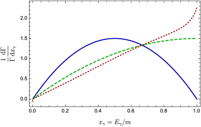
(a)

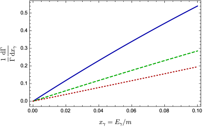
(b)

Figure 2: The photon spectrum of $\text{p-Ps}\to\gamma\nu_{\ell}\bar{\nu}_{\ell}$ (solid), $\text{o-Ps}\to\gamma\nu_{\ell}\bar{\nu}_{\ell}$ (dashed) and $\text{o-Ps}\to 3\gamma$ (dotted) decays plotted over LABEL:sub@fig:spectrum_a the full energy domain of the photon, $x_{\gamma}\in(0,1)$ and LABEL:sub@fig:spectrum_b over the low-energy domain $x_{\gamma}\in(0,0.1)$.

When the photon reaches the maximum energy, $x_{\gamma}=1$, the neutrino (left-handed) and the antineutrino (right-handed) move collinearly in the direction opposite to the photon. Their spins cancel and the angular momentum of the system is carried by the photon’s spin. Clearly, this is possible only for o-Ps; for this reason, the p-Ps spectrum vanishes at $x_{\gamma}=1$ (Fig. LABEL:sub@fig:spectrum_a). This spectrum also vanishes at $x_{\gamma}=0$. However, the p-Ps spectrum of Ref. Pérez-Ríos and Love (2015) vanishes at neither $x_{\gamma}=0$ or $x_{\gamma}=1$.

The p-Ps spectrum is maximal at $x_{\gamma}=1/2$; different from the maximum $x_{\gamma}=2/3$, predicted in Pérez-Ríos and Love (2015). On the other hand the o-Ps spectrum is maximal at $x_{\gamma}=1$ when the photon carries whole angular momentum of the system.

We also note that the spectra we have found (neglecting binding effects) are linear in the low-energy limit (Fig. LABEL:sub@fig:spectrum_b). Since Low’s theorem Low (1958) predicts the low-energy behaviour of the spectrum to be cubic rather than linear, we shall determine how binding effects modify the results (9) and (10) (Sec. IV).

III Angular Distributions of $\boldsymbol{\text{Ps}\to\gamma\nu_{\ell}\bar{\nu}_{\ell}}$ Decays

In Sec. II, we calculated the decay rates and spectra for p-Ps and o-Ps, and found that both can decay into a photon and a neutrino-antineutrino pair. To better understand these decays, we calculate the angular dependence of the $\text{Ps}\to\gamma\nu_{\ell}\bar{\nu}_{\ell}$ amplitudes (Sec. III.1) and then use those amplitudes to determine the angular distributions of $\text{Ps}\to\gamma\nu_{\ell}\bar{\nu}_{\ell}$ decays (Sec. III.2).

III.1 Angular Dependence of the Decay Amplitudes

The angular dependence of the decay amplitudes is most easily found by reformulating the three-body decay $\text{Ps}\to\gamma\nu_{\ell}\bar{\nu}_{\ell}$, in terms of a two-body decay $\text{Ps}\to\gamma Z^{*}$, where $Z^{*}$ is a massive vector boson of polarization $\epsilon$ and 4-momentum $q$. Specifically, the three-body phase space of the decay rate is factorized into two two-body phase spaces (one for $\text{Ps}\to\gamma Z^{*}$ and one for $Z^{*}\to\nu\bar{\nu}$) and an integral over the invariant mass squared of the $Z^{*}$ boson. After integrating over the neutrino momenta, the $\text{Ps}\to\gamma\nu_{\ell}\bar{\nu}_{\ell}$ decay rate can be written as the integral of the $\text{Ps}\to\gamma Z^{*}$ decay rate (multiplied by a factor from the $Z^{*}\to\nu\bar{\nu}$ phase space) over the invariant mass of $Z^{*}$ squared (Appendix A),

$$\Gamma_{\text{p/o}}=\frac{\text{G}_{\text{F}}^{2}}{2\pi^{2}\alpha}\int\frac{\text{d}q^{2}}{2\pi}q^{2}\Gamma_{\text{(p/o)-Ps}\to\gamma Z^{*}},$$ (11)

where $q=k_{1}+k_{2}$ is the $Z^{*}$ 4-momentum and

$$\Gamma_{\text{(p/o)-Ps}\to\gamma Z^{*}} = \frac{1}{g}\frac{1}{2m_{\text{Ps}}}\int\text{d}\Phi_{2}\left(p_{1}+p_{2};q,k_{\gamma}\right)\frac{\left|\psi_{0}(0)\right|^{2}}{m}\frac{1}{3}\sum_{\text{spin/pol}}\left|\mathcal{M}_{\text{(p/o)-Ps}\to\gamma Z^{*}}\right|^{2}.$$ (12)

Here, $g$ is the number of polarizations of the initial Ps state.

From (11), it is clear that the three-body problem $\text{Ps}\to\gamma\nu_{\ell}\bar{\nu}_{\ell}$ can be described in terms of the two-body problem $\text{Ps}\to\gamma Z^{*}$. The $Z^{*}$ couples to the electron current through both vector and axial-vector coupling with the Feynman rule $ie\cancel{\epsilon}^{*}\left(v_{\ell}-a_{\ell}\gamma^{5}\right)$ at each $e^{\pm}Z^{*}$ vertex.

To construct the angular dependence of the $\text{Ps}\to\gamma Z^{*}$ decay amplitudes on the spherical angles $\theta$ and $\phi$, we first determine the decay amplitudes to final states where the photon moves along the $+z$-axis and the $Z^{*}$ boson moves along the $-z$-axis. The angular dependence is then determined by rotating the initial state and considering decay along the new $z^{\prime}$-axis Feynman et al. (1963). Alternatively, one can obtain the angular dependence using the helicity basis formalism of Refs. Jacob and Wick (1959); Richman (1984); Leader (2011); Chung (1971).

The $\text{p-Ps}\to\gamma Z^{*}$ decay amplitudes are isotropic and given by

$$\mathcal{A}_{m^{\prime}_{\gamma},m^{\prime}_{Z}}(\theta,\phi)=\mathcal{A}_{m^{\prime}_{\gamma},m^{\prime}_{Z}}\propto\delta_{m^{\prime}_{\gamma},-m^{\prime}_{Z}},$$ (13)

where $m_{\gamma}^{\prime}\in\{\pm 1\}$ and $m_{Z}^{\prime}\in\{\pm 1,0\}$ are the spin projections of the photon and $Z^{*}$ along the $z^{\prime}$-axis. The $z^{\prime}$-axis points along the photon trajectory defined by the spherical polar angles $\theta$ and $\phi$ in the original unrotated frame. The p-Ps amplitudes were calculated and are listed in Table 1.

Table 1: The $\text{p-Ps}\to\gamma Z^{*}$ decay amplitudes, $\mathcal{A}_{m_{\gamma}^{\prime}m_{Z}^{\prime}}/v_{\ell}e^{2}$, as a function of the spherical angles $\theta$ and $\phi$. Since p-Ps is odd under parity, $\mathcal{A}_{-m_{\gamma}^{\prime}-m_{Z}^{\prime}}=-\mathcal{A}_{m_{\gamma}^{\prime}m_{Z}^{\prime}}$; therefore, only the $m_{\gamma}^{\prime}=+1$ amplitudes need be tabulated.

	$+1$	$0$	$-1$
$+1$	$0$	$0$	$4i/\sqrt{2}$

The $\text{o-Ps}\to\gamma Z^{*}$ amplitudes must be calculated for each initial polarization of o-Ps. In the initial frame before decay, the o-Ps atom is in a state of definite angular momentum with some spin projection along the $z$-axis. We let $|\Lambda\rangle$ represent this initial state. The o-Ps atom subsequently decays along the $z^{\prime}$-axis with the amplitude $\mathcal{A}_{m_{\gamma}^{\prime}m_{Z}^{\prime}}^{m_{\Lambda}}$ where $m_{\Lambda}\in\{\pm 1,0\}$ is the initial spin projection of o-Ps along the $z$-axis. The o-Ps amplitudes are derived in Appendix B and are listed in Table 2.

Table 2: The $\text{o-Ps}\to\gamma Z^{*}$ decay amplitudes, $\mathcal{A}_{m_{\gamma}^{\prime}m_{Z}^{\prime}}^{m_{\Lambda}}/a_{\ell}e^{2}$, as a function of the spherical angles $\theta$ and $\phi$ evaluated at $\mathbf{q}=-\mathbf{k}_{\gamma},E_{Z}=2m-E_{\gamma}$. The $m_{\Lambda}=-1$ amplitudes can be obtained from the $m_{\Lambda}=+1$ amplitudes by the replacment $\theta\to\theta+\pi$ and $\phi\to-\phi$.

$m_{\Lambda}$		$+1$	$0$	$-1$
$+1$	$+1$	0	$\sqrt{2}(1+\cos\theta)e^{i\phi}/\sqrt{1-x_{\gamma}}$	$-2i\sin\theta e^{i\phi}$
	$-1$	$2i\sin\theta e^{i\phi}$	$-\sqrt{2}(1-\cos\theta)e^{i\phi}/\sqrt{1-x_{\gamma}}$	0
$0$	$+1$	0	$2\sin\theta/\sqrt{1-x_{\gamma}}$	$4i\cos\theta/\sqrt{2}$
	$-1$	$-4i\cos\theta/\sqrt{2}$	$-2\sin\theta/\sqrt{1-x_{\gamma}}$	0

To validate the amplitudes in Tables 1 and 2, we use them to calculate the decay rates and photon spectra, and compare these with those obtained in Sec. II. To do this, we first derive the spin averaged amplitudes squared. For p-Ps, this task is simple,

$$\frac{1}{3}\sum_{m_{\gamma}^{\prime}m_{Z}^{\prime}}\left|\mathcal{A}_{m_{\gamma}m_{Z}^{\prime}}\right|_{\mathbf{q}=-\mathbf{k}_{\gamma},E_{Z}=2m-E_{\gamma}}^{2}=\frac{16v_{\ell}^{2}e^{4}}{3}.$$ (14)

To obtain the o-Ps spin averaged amplitude squared, it is convenient to first sum over $m_{\Lambda}$ and $m_{\gamma}^{\prime}$

$$\sum_{m_{\Lambda}m_{\gamma}^{\prime}}\left|\mathcal{A}_{m_{\gamma}+}^{m_{\Lambda}}\right|_{\mathbf{q}=-\mathbf{k}_{\gamma},E_{Z}=2m-E_{\gamma}}^{2} = \sum_{m_{\Lambda}m_{\gamma}^{\prime}}\left|\mathcal{A}_{m_{\gamma}-}^{m_{\Lambda}}\right|_{\mathbf{q}=-\mathbf{k}_{\gamma},E_{Z}=2m-E_{\gamma}}^{2}=8a_{\ell}^{2}e^{4},$$ (15)

$$\sum_{m_{\Lambda}m_{\gamma}^{\prime}}\left|\mathcal{A}_{m_{\gamma}0}^{m_{\Lambda}}\right|_{\mathbf{q}=-\mathbf{k}_{\gamma},E_{Z}=2m-E_{\gamma}}^{2} = \frac{16a_{\ell}^{2}e^{4}}{m-E_{\gamma}}.$$ (16)

Then completing the sum over $m_{Z}^{\prime}$ and dividing by the number of o-Ps and $Z^{*}$ polarizations yields the spin averaged amplitude squared

$$\frac{1}{3\cdot 3}\sum_{m_{\Lambda}m_{\gamma}^{\prime}m_{Z}^{\prime}}\left|\mathcal{A}_{m_{\gamma}m_{Z}^{\prime}}^{m_{\Lambda}}\right|_{\mathbf{q}=-\mathbf{k}_{\gamma},E_{Z}=2m-E_{\gamma}}^{2}=\frac{16a_{\ell}^{2}e^{4}}{9}\frac{2-x_{\gamma}}{1-x_{\gamma}}.$$ (17)

The decay rates and spectra are calculated by substituting equations (14) and (17) into (11). Since the spin averaged amplitudes squared are independent of $\theta$ and $\phi$, the angular integrations of (11) are easy and yield

$$\Gamma_{\text{p/o}} = \frac{4\text{G}_{\text{F}}^{2}m^{5}\alpha^{4}}{3\pi^{3}}\int_{0}^{1}\text{d}x\;\left\{\begin{matrix}v_{\ell}^{2}x_{\gamma}(1-x_{\gamma})\\ a_{\ell}^{2}x_{\gamma}(2-x_{\gamma})/3\\ \end{matrix}\right\}$$ (18)

$$= \frac{4\text{G}_{\text{F}}^{2}\alpha^{4}m^{5}}{9\pi^{3}}\left\{\begin{matrix}v_{\ell}^{2}/2\\ 2a_{\ell}^{2}/3\\ \end{matrix}\right\},$$ (19)

where the top (bottom) line in the curly brackets is used for the p-Ps (o-Ps) decay rate. The decay rates (19) are identical to (4) and (5). The spectra are the integrands of equation (18) and are also equal to the spectra (9) and (10). Thus, the amplitudes of Tables 1 and 2 are consistent with our results from Sec. II.

While it is evident that p-Ps and o-Ps cannot decay into the same final states (even though they have the same constituent particles), we confirm the orthogonality of the p-Ps and o-Ps decay amplitudes. The o-Ps amplitudes, $\mathcal{A}^{m_{\Lambda}}_{\pm^{\prime}0^{\prime}}$, are trivially orthogonal to the p-Ps amplitudes (13) because p-Ps cannot decay into a longitudinally polarized $Z^{*}$ and photon. To check the orthogonality of $\mathcal{A}^{m_{\Lambda}}_{\pm^{\prime}\mp^{\prime}}$ with (13), we take their inner product

$$\int\text{d}\Omega\mathcal{A}_{m_{\gamma},m_{Z}}\left(\mathcal{A}_{\pm^{\prime}\mp^{\prime}}^{m_{\Lambda}}\left(\theta,\phi\right)\right)^{*}\propto\int\text{d}\Omega\left(\mathcal{A}_{\pm^{\prime}\mp^{\prime}}^{m_{\Lambda}}\left(\theta,\phi\right)\right)^{*}.$$ (20)

Since $\mathcal{A}_{\pm^{\prime}\mp^{\prime}}^{m_{\Lambda}}\left(\theta,\phi\right)$ are proportional to $e^{\pm i\phi}$ or $\cos\theta$ (depending on $m_{\Lambda}$), the inner products vanish proving orthogonality; this is as expected because $\mathcal{A}_{\pm^{\prime}\mp^{\prime}}^{m_{\Lambda}}\left(\theta,\phi\right)$ (Table 2) are p-waves while the p-Ps amplitudes are s-waves (Table 1).

Thus, the $\text{p-Ps}\to\gamma\nu_{\ell}\bar{\nu}_{\ell}$ and $\text{o-Ps}\to\gamma\nu_{\ell}\bar{\nu}_{\ell}$ decays do not have access to the same final state despite the fact that the final states contain the same constituent particles.

III.2 Angular Distributions

The angular distribution for a specific $\gamma+Z^{*}$ final state is found by differentiating the decay amplitude (11), where the squared amplitude corresponding to the specific final state (Tables 1 and 2) is used in place of the spin averaged amplitude squared, by $x_{\gamma}$ and $\cos\theta$.

Since the p-Ps amplitudes are isotropic, the $\text{p-Ps}\to\gamma\nu_{\ell}\bar{\nu}_{\ell}$ angular distributions are also isotropic ($9\Gamma_{\text{p}}x_{\gamma}(1-x_{\gamma})/2$ for $m_{\gamma}^{\prime}=\pm 1$). Thus, p-Ps is equally likely to decay into a photon and a neutrino-antineutrino pair where the photon is emitted in any direction.

The $\text{o-Ps}\to\gamma\nu_{\ell}\bar{\nu}_{\ell}$ angular distributions are determined to be

$$\frac{1}{\Gamma_{\text{o}}}\frac{\text{d}^{2}\Gamma_{m_{\gamma}^{\prime}m_{Z}^{\prime}}^{m_{\Lambda}}}{\text{d}x_{\gamma}\text{d}\cos\theta}=\frac{27}{64}x_{\gamma}(1-x_{\gamma})\int\frac{\text{d}\phi}{2\pi}\left|\frac{\mathcal{A}_{m_{\gamma}^{\prime}m_{Z}^{\prime}}^{m_{\Lambda}}}{a_{\ell}e^{2}}\right|_{\mathbf{q}=-\mathbf{k}_{\gamma},E_{Z}=2m-E_{\gamma}}^{2},$$ (21)

and are tabulated in Table 3. Since $Z^{*}$ is a mathematical convenience, the physical angular distributions for a given o-Ps polarization $m_{\Lambda}$ and photon helicity $m_{\gamma}^{\prime}$ is obtained by averaging over the $Z^{*}$ polarizations. For an o-Ps atom initially polarized in the $m_{\Lambda}=0$ state, the angular distributions for decay into a photon of helicity $m_{\gamma}^{\prime}\pm 1$ are $9\Gamma_{\text{o}}(\sin^{2}\theta x_{\gamma}+2\cos^{2}\theta x_{\gamma}(1-x_{\gamma}))/16$ and non-zero for all $\theta$. The angular distribution for o-Ps initially polarized in the $m_{\Lambda}=+1$ state decaying into a photon of helicity $m_{\gamma}^{\prime}=+1$ is $9\Gamma_{\text{o}}(2\cos^{4}(\theta/2)x_{\gamma}+\sin^{2}\theta x_{\gamma}(1-x_{\gamma}))/16$; since this angular distribution vanishes for $\theta=\pi$, an o-Ps atom in the $m_{\Lambda}=+1$ state cannot decay into a photon of helicity $m_{\gamma}^{\prime}=+1$ along the $-z$-axis. Similarly, an o-Ps atom initially polarized in the $m_{\Lambda}=+1$ state cannot decay into a photon of helicity $m_{\gamma}^{\prime}=-1$ along the $+z$-axis.

Table 3: The angular distributions for $\text{o-Ps}\to\gamma\nu_{\ell}\bar{\nu}_{\ell}$ decays, $(\text{d}^{2}\Gamma_{m_{\gamma}^{\prime}m_{Z}^{\prime}}^{m_{\Lambda}}/\text{d}x_{\gamma}\text{d}\cos\theta)/\Gamma_{\text{o}}$. The $m_{\Lambda}=-1$ distributions can be obtained from the $m_{\Lambda}=+1$ angular distributions by the replacement $\theta\to\theta+\pi$ and $\phi\to-\phi$.

$m_{\Lambda}$		$+1$	$0$	$-1$
$+1$	$+1$	0	$27\cos^{4}(\theta/2)x_{\gamma}/8$	$27\sin^{2}\theta x_{\gamma}(1-x_{\gamma})/16$
	$-1$	$27\sin^{2}\theta x_{\gamma}(1-x_{\gamma})/16$	$27\sin^{4}(\theta/2)x_{\gamma}/8$	0
$0$	$+1$	0	$27\sin^{2}\theta x_{\gamma}/16$	$27\cos^{2}\theta x_{\gamma}(1-x_{\gamma})/8$
	$-1$	$27\cos^{2}\theta x_{\gamma}(1-x_{\gamma})/8$	$27\sin^{2}\theta x_{\gamma}/16$	0

The photon spectrum for a specific $\gamma+Z^{*}$ final state is calculated by integrating the corresponding angular distribution by $\text{d}\cos\theta$. These spectra are listed in Tables 4 and 5 and provides further insight into equations (9) and (10).

Table 4: $\text{p-Ps}\to\gamma\nu_{\ell}\bar{\nu}_{\ell}$ photon spectra, $(\text{d}\Gamma_{\text{p}}/\text{d}x_{\gamma})/\Gamma_{\text{p}}$, for specific $\gamma+Z^{*}$ final states. Since $|\mathcal{A}_{m_{\gamma}^{\prime}m_{Z}^{\prime}}|^{2}=|\mathcal{A}_{-m_{\gamma}^{\prime}-m_{Z}^{\prime}}|^{2}$, only the $m_{\gamma}^{\prime}=+1$ decay rates need be tabulated.

	$+1$	$0$	$-1$
$+1$	$0$	$0$	$9x_{\gamma}(1-x_{\gamma})$

Table 5: $\text{o-Ps}\to\gamma\nu_{\ell}\bar{\nu}_{\ell}$ photon spectra, $(\text{d}\Gamma_{\text{o}}/\text{d}x_{\gamma})/\Gamma_{\text{o}}$, for specific $\gamma+Z^{*}$ final states and any $m_{\Lambda}$.

	$+1$	$0$	$-1$
$+1$	0	$9x_{\gamma}$ /4	$9x_{\gamma}(1-x_{\gamma})/4$
$-1$	$9x_{\gamma}(1-x_{\gamma})/4$	$9x_{\gamma}/4$	0

The photon spectrum of decays to final states with $m_{\gamma}^{\prime}=\pm$ and $m_{Z}^{\prime}=\mp$ are proportional to $x_{\gamma}\left(1-x_{\gamma}\right)$ and vanish as $x_{\gamma}\to 1$. On the other hand, the photon spectrum of decays to final states with $m_{\gamma}^{\prime}=\pm$ and $m_{Z}^{\prime}=0$ are linear and maximal at $x_{\gamma}\to 1$. The o-Ps photon spectrum is maximal at $x_{\gamma}=1$ because the o-Ps decay has access to two additional final states with a longitudinally polarized $Z^{*}$; these add to the linear term in the spectrum. The $\mathcal{A}^{m_{\Lambda}}_{\pm 0}$ amplitudes contain a factor of $2m/q=1/\sqrt{1-x_{\gamma}}$ from the longitudinal polarization of $Z^{*}$. This factor enhances the amplitude for high-energy photons and cancels the factor $q^{2}\propto\left(1-x_{\gamma}\right)$ in the $\text{d}q^{2}$ integral of (11). In the high-energy limit, $x_{\gamma}\to 1$, the longitudinal polarization of $Z^{*}$ represents a final state where the neutrino and antineutrino are collinear.

IV Low’s theorem and the Soft Photon Limit of the Spectra

Low’s theorem Low (1958) places constraints on the amplitude of any radiative process and predicts the spectrum in the soft photon limit. In Sec. II, the tree level electroweak photon spectra, equations (9) and (10), were found to be linear in the low-energy limit, similar to the Ore-Powell $\text{o-Ps}\to 3\gamma$ spectrum. However, it was pointed out by Ref. Pestieau and Smith (2002) that the Ore-Powell spectrum is in contradiction with Low’s theorem. Therefore, it is important to reconcile equations (9) and (10) with Low’s theorem.

Low’s theorem states that the $\mathcal{O}(E^{-1}_{\gamma})$ and $\mathcal{O}(E^{0}_{\gamma})$ terms in the Laurent expansion of the radiative amplitude, $X\to Y+\gamma$, are obtained from knowledge of the non-radiative amplitude, $X\to Y$ Manohar and Ruiz-Femenia (2004); Low (1958); Pestieau and Smith (2002). Expanding the radiative amplitude, $\epsilon_{\gamma}^{\mu}\mathcal{M}_{\mu}$, in a Laurent series in the photon energy, we obtain

$$\epsilon_{\gamma}^{\mu}\mathcal{M}_{\mu}=\sum_{n=-1}^{\infty}\mathcal{M}_{n}E^{n}_{\gamma},$$ (22)

where $\mathcal{M}_{i}$ is the coefficient of the $\mathcal{O}\left(E^{i-1}_{\gamma}\right)$ term of the Laurent series. The coefficients $\mathcal{M}_{0}$ and $\mathcal{M}_{1}$ are independent of $E_{\gamma}$ and determined by the non-radiative amplitude, its derivatives in physically allowed regions and the anomalous magnetic moments of the particles involved in the reaction Low (1958).

The $\mathcal{M}_{0}$ coefficient is proportional to the non-radiative amplitude multiplied by the factor $-Q_{i}\epsilon\cdot p_{i}/k_{\gamma}\cdot p_{i}$, which arises from the emission of a photon by an outgoing or ingoing particle Manohar and Ruiz-Femenia (2004). The $\mathcal{M}_{0}$ coefficient vanishes when there are no moving charged particles in the initial and final state of the non-radiative process or when the non-radiative amplitude is zero. The coefficient $\mathcal{M}_{1}$ is a function of the magnetic moments of the particles as well as the non-radiative amplitude and its derivatives with respect energy and angle Low (1958).

By combining the behavior of the radiative amplitude and the phase space, we find that the low-energy photon spectrum has the form

$$\frac{\text{d}\Gamma}{\text{d}E_{\gamma}}=\frac{A}{E_{\gamma}}+B+CE_{\gamma}+DE_{\gamma}^{2}+\mathcal{O}\left(E_{\gamma}^{3}\right),$$ (23)

where

$$A = |\mathcal{M}_{0}|^{2}$$

$$B = \mathcal{M}_{0}\mathcal{M}_{1}^{*}+\mathcal{M}_{1}\mathcal{M}_{0}^{*}$$

$$C = \left|\mathcal{M}_{1}\right|^{2}+\mathcal{M}_{0}\mathcal{M}_{2}^{*}+\mathcal{M}_{2}\mathcal{M}_{0}^{*}$$

$$D = \mathcal{M}_{0}\mathcal{M}_{\gamma}^{*}+\mathcal{M}_{\gamma}\mathcal{M}_{0}^{*}+\mathcal{M}_{1}\mathcal{M}_{2}^{*}+\mathcal{M}_{2}\mathcal{M}_{1}^{*}.$$ (24)

If $\mathcal{M}_{0}$ vanishes, then $A=B=0$ and the soft photon spectrum is of order $E_{\gamma}\text{d}E_{\gamma}$. If both $\mathcal{M}_{0}$ and $\mathcal{M}_{1}$ vanish, then $A=B=C=D=0$ and the soft photon spectrum is of order $E_{\gamma}^{3}\text{d}E_{\gamma}$.

For $\text{p-Ps}\to\gamma\nu_{\ell}\bar{\nu}_{\ell}$, the non-radiative $\text{p-Ps}\to\nu_{\ell}\bar{\nu}_{\ell}$ amplitude vanishes Czarnecki and Karshenboim (2000); application of Low’s theorem yields $\mathcal{M}_{0,1}=0$ for the radiative decay, $\text{p-Ps}\to\gamma\nu_{\ell}\bar{\nu}_{\ell}$. Since the radiative $\text{o-Ps}\to\gamma\nu_{\ell}\bar{\nu}_{\ell}$ decay proceeds only via axial-vector coupling while the non-radiative $\text{o-Ps}\to\nu_{\ell}\bar{\nu}_{\ell}$ amplitude is proportional to vector coupling Czarnecki and Karshenboim (2000), Low’s theorem requires that the $\mathcal{O}(E^{-1}_{\gamma})$ and $\mathcal{O}(E^{0}_{\gamma})$ terms of the radiative $\text{o-Ps}\to\gamma\nu_{\ell}\bar{\nu}_{\ell}$ amplitude vanish $(i.e.,\mathcal{M}_{0,1}=0$). Thus, for both $\text{Ps}\to\gamma\nu_{\ell}\bar{\nu}_{\ell}$ decays, Low’s theorem predicts that the photon spectra are cubic in the low-energy limit in apparent contradiction with equations (9) and (10).

Equations (9) and (10) were calculated using the tree level electroweak amplitude for the $e^{+}e^{-}\to\gamma\nu_{\ell}\bar{\nu}_{\ell}$ annihilation multiplied by the probability density for the $e^{+}e^{-}$ pair to be at the origin. This calculation assumes that the electron and positron are initially free and at rest, and therefore neglects the binding effects in Ps. Binding effects are of order $m\alpha^{2}$. For photons with comparable energies, binding effects become important and equations (9) and (10) are no longer accurate.

To resolve the contradiction between equations (9) and (10), and Low’s theorem, we must include binding effects in the soft photon spectrum of $\text{Ps}\to\gamma\nu_{\ell}\bar{\nu}_{\ell}$ decays. To do this we employ the NREFT methods developed in Refs. Manohar and Ruiz-Femenia (2004); Ruiz-Femenia (2008); Voloshin (2004).

V Soft Photon Decay Spectra

NREFTs provide a systematic way of incorporating binding effects in the computation of bound state decay amplitudes. One computes the decay amplitudes in electroweak theory. Then a NREFT Hamiltonian is constructed to reproduce the soft photon limit of the electroweak amplitudes when ignoring binding effects. In other words, the effective theory dynamics (ignoring binding effects) are set equal to the low-energy limit of the electroweak dynamics. The soft-photon limit of the electroweak amplitudes are calculated in Sec. V.1. They are used in Secs. V.3 and V.4 to calculate the matching condition used to verify that the effective theory amplitudes (without binding) are indeed equal to the soft photon limit of the electroweak amplitudes.

Once this matching has been performed, the NREFT Hamiltonian is used to calculate the effective theory amplitudes and subsequently the soft photon spectra. The effective theory amplitudes are calculated using time-ordered perturbation theory and have both long (Coulomb) and short distance (annihilation into a $\nu_{\ell}\bar{\nu}_{\ell}$ pair) contributions.

The Coulomb ($H_{C}$) and Coulomb interaction ($H_{\text{int}}$) Hamiltonians describe the bound state dynamics of an $e^{+}e^{-}$ pair interacting with a quantized electromagnetic field. Following Ref. Voloshin (2004), we argue that the dipole approximation of the Coulomb interaction Hamiltonian is valid in the energy range $E_{\gamma}\ll m$ (Sec. V.2). In the dipole approximation, the Coulomb Hamiltonians are

$$H = H_{\text{C}}+H_{\text{int}},$$ (25)

$$H_{\text{C}} = \frac{\mathbf{p}^{2}}{m}-\frac{\alpha}{r},$$ (26)

$$H_{\text{int}} = -e\mathbf{x}\cdot\mathbf{E}-\mu\left[\boldsymbol{\sigma}_{\phi}+\boldsymbol{\sigma}_{\chi}\right]\cdot\mathbf{B},$$ (27)

in terms of the center of mass variables $\mathbf{p}=\left(\mathbf{p}_{1}-\mathbf{p}_{2}\right)/2$ and $\mathbf{x}=\mathbf{x}_{1}-\mathbf{x}_{2}$ where the subindices 1, 2 refer to the electron and positron Manohar and Ruiz-Femenia (2004). Here, $\boldsymbol{\sigma}_{\phi/\chi}$ are the Pauli matrices acting on the electron ($\phi$) and positron ($\chi$) spinors. The electric, $\mathbf{E}$ and magnetic, $\mathbf{B}$, fields are evaluated in the dipole approximation and $H_{\text{int}}$ can induce both E1 and M1 transitions within the Ps atom.

The Coulomb Hamiltonian $H_{C}$ is the leading term in the velocity of the electron $v\ll 1$. The Coulomb interaction Hamiltonian, $H_{\text{int}}$, is higher order in $v$ and taken as a perturbation. The (p/o)-Ps annihilation amplitude is given by the first order $v$ expansion of the electroweak $e^{+}e^{-}\to\nu_{\ell}\bar{\nu}_{\ell}$ annihilation amplitude calculated in Appendix C. While the neutrino energies are of order $\mathcal{O}(m)$, a non-relativistic treatment is still valid since the annihilation into a neutrino-antineutrino pair is a short distance effect – the neutrinos are not dynamical.

V.1 Soft Photon Limit of the Tree Level Electroweak Decay Amplitude

Using the standard Feynman rules, the $\text{Ps}\to\gamma\nu\bar{\nu}$ decay amplitude (Fig. 1) is

$$\mathcal{M}=-2\sqrt{2}i\text{G}_{\text{F}}em\bar{v}\left(p_{2}\right)\left(\cancel{J}\left(v_{\ell}-a_{\ell}\gamma^{5}\right)\frac{\cancel{p}_{1}-\cancel{k}_{\gamma}+m}{(p_{1}-k_{\gamma})^{2}-m^{2}}\cancel{\epsilon}_{\gamma}^{*}+\cancel{\epsilon}_{\gamma}^{*}\frac{\cancel{k}_{\gamma}-\cancel{p}_{2}+m}{(k_{\gamma}-p_{2})^{2}-m^{2}}\cancel{J}\left(v_{\ell}-a_{\ell}\gamma^{5}\right)\right)u\left(p_{1}\right),$$ (28)

where $J^{\mu}\left(k_{1},k_{2}\right)=\bar{u}(k_{1})\gamma^{\mu}\left(1-\gamma^{5}\right)v(k_{2})$ is the neutrino current, $p_{1}$ and $p_{2}$ are the electron and positron 4-momenta, $k_{1}$ and $k_{2}$ are the neutrino and antineutrino 4-momenta, $k_{\gamma}$ is the photon 4-momentum and $\epsilon_{\gamma}$ is the photon polarization.

We choose the Dirac representation for the electron and positron spinors in (28). In this representation, the electron spinor is

$$u_{s}(\mathbf{p})=\frac{1}{\sqrt{E+m}}\left(\begin{array}[]{c}E+m\\ \mathbf{p}\cdot\boldsymbol{\sigma}\end{array}\right)\phi_{s},$$ (29)

where $E=\sqrt{m^{2}+\mathbf{p}^{2}}$, $\phi_{s}$ is the two-component electron spinor and the index $s$ denotes the spin projection Dick (2016). The positron spinors are related to the electron spinors by charge conjugation,

$$v_{s}\left(\mathbf{p}\right)=\frac{1}{\sqrt{E+m}}\left(\begin{array}[]{c}\mathbf{p}\cdot\boldsymbol{\sigma}\\ E+m\end{array}\right)\chi_{s},$$ (30)

where $\chi_{s}$ is the two-component spinor of the positron.

Since the Ps binding energy is small, $\mathcal{O}(m\alpha^{2})$, the typical momentum of the electron is small and we neglect it (i.e., $p_{1}=p_{2}=(m,\mathbf{0})$). In the limit $E_{\gamma}\to 0$, the neutrino momenta are back to back ($\mathbf{k}_{1}=-\mathbf{k}_{2}$) and $J^{0}\to 0$. Factoring out the $E_{\gamma}$ dependence and working with $\hat{\mathbf{k}}_{\gamma}=\mathbf{k}_{\gamma}/E_{\gamma}$, equation (28) becomes

$$\mathcal{M}=2\sqrt{2}\text{G}_{\text{F}}e\chi^{\dagger}\left(v_{\ell}\left(\hat{\mathbf{k}}_{\gamma}\times\boldsymbol{\epsilon}_{\gamma}\right)\cdot\mathbf{J}+a_{\ell}\left(\boldsymbol{\epsilon}_{\gamma}\times\mathbf{J}\right)\cdot\boldsymbol{\sigma}\right)\phi,$$ (31)

where we choose $\epsilon_{\gamma}$ to be real and transverse to $k_{\gamma}$. Projecting the electron and positron spinors onto the p-Ps ($\chi^{\dagger}\phi\to\sqrt{2}$ and $\chi^{\dagger}\boldsymbol{\sigma}\phi\to\mathbf{0}$) and o-Ps ($\chi^{\dagger}\phi\to 0$ and $\chi^{\dagger}\boldsymbol{\sigma}\phi\to\sqrt{2}\boldsymbol{\xi}$) states, the low-energy limit of the electroweak amplitudes are

$$\mathcal{M}_{\text{p}} = 4\text{G}_{\text{F}}ev_{\ell}\left(\boldsymbol{\epsilon}_{\gamma}\times\mathbf{J}\right)\cdot\hat{\mathbf{k}}_{\gamma},$$ (32)

$$\mathcal{M}_{\text{o}} = 4\text{G}_{\text{F}}ea_{\ell}\left(\boldsymbol{\epsilon}_{\gamma}\times\mathbf{J}\right)\cdot\boldsymbol{\xi},$$ (33)

where $\boldsymbol{\xi}$ is the o-Ps polarization vector.

V.2 Dipole Approximation of the Coulomb Interaction Hamiltonian

While normally the dipole approximation is applicable for photons with wavelengths much larger than the spatial extent of the Ps atom, $2/m\alpha$ (i.e., $E_{\gamma}\ll m\alpha$), it has been shown that the dipole approximation of the Coulomb interaction Hamiltonian holds in the enlarged energy region $E_{\gamma}\ll m$ for the three-body decay $\text{o-Ps}\to 3\gamma$ Voloshin (2004); Ruiz-Femenia (2008). In this energy region, amplitudes where the intermediate states propagate via the Coulomb Green’s function, are a series in $\alpha\sqrt{m/E_{\gamma}}\sim\sqrt{\alpha}$ rather than integer powers of $\alpha$. The main contributions to the effective field theory amplitudes arise from distances of order $\mathcal{O}(1/\sqrt{mE_{\gamma}})$, which are much smaller than the Ps radius $\mathcal{O}(1/m\alpha)$ Ruiz-Femenia (2008). We argue that the same considerations apply to $\text{Ps}\to\gamma\nu_{\ell}\bar{\nu}_{\ell}$ decays and that the dipole approximation holds in the extended energy range $E_{\gamma}\ll m$.

Initially, the Ps atom is in either the ${}^{1}S_{0}$ or ${}^{3}S_{1}$ states at energy $E_{0}=-m\alpha^{2}/4$ relative to the threshold. The p-Ps (o-Ps) atom then emits a soft photon and the $e^{+}e^{-}$ pair propagates non-relativistically in the Coulomb field in a C-odd (C-even) state of energy $E_{0}-E_{\gamma}$ before annihilating into a neutrino-antineutrino pair (Fig. 3).

(a)

(b)

Figure 3: Effective theory graphs for LABEL:sub@fig:p-Ps_soft_gnn $\text{p-Ps}\to\gamma\nu_{\ell}\bar{\nu}_{\ell}$ and LABEL:sub@fig:o-Ps_soft_gnn $\text{o-Ps}\to\gamma\nu_{\ell}\bar{\nu}_{\ell}$. The open square (circle) represents a M1 (E1) transition while the solid star represents the annihilation of o-Ps into a neutrino-antineutrino pair.

The Green’s function of the $e^{+}e^{-}$ pair, interacting via a Coulomb field, $G_{C}$, describes the propagation of the pair between the emission of the soft photon and the annihilation into a neutrino-antineutrino pair. It satisfies the equation

$$\left(H_{C}+\frac{\kappa^{2}}{m}\right)G_{C}({\bf x},{\bf y};\kappa)=\delta\left({\bf x}-{\bf y}\right)$$ (34)

and has a factor $\exp\left(-\kappa r\right)$ with $-\kappa^{2}/m=E_{\gamma}$. Therefore, the virtual pair propagates over a distance of $\mathcal{O}(\kappa^{-1})$ Voloshin (2004).

Since the spin-singlet state cannot annihilate into a neutrino-antineutrino pair Czarnecki and Karshenboim (2000), the virtual C-odd (C-even) state of Fig. LABEL:sub@fig:p-Ps_soft_gnn (LABEL:sub@fig:o-Ps_soft_gnn) must be a triplet state of orbital angular momentum $L=2n$ ($L=2n+1$) for $n$ a non-negative integer. The amplitude for annihilation contains $L$ derivatives of the wave function at the origin and is proportional to $(\kappa/m)^{L}$. Since the $\exp(-\kappa r)$ dependence of the Green’s function constrains the product $E_{\gamma}r$ to order one, the contributions of the intermediate states of Fig. 3 to the amplitude are proportional to $(E_{\gamma}/m)^{L}$.

Therefore, only the intermediate states with the lowest $n$ (i.e., $n=0$) need to be considered for $E_{\gamma}\ll m$ Voloshin (2004). The intermediate state of Fig. LABEL:sub@fig:p-Ps_soft_gnn is the o-Ps ground state, $1^{3}S_{1}$, while the intermediate states of Fig. 3b are the $L=1$ o-Ps excited states, $n^{3}P_{0,1,2}$. These states are reached from the initial p-Ps and o-Ps ground states by M1 and E1 transitions respectively. Thus, the dipole approximation is valid in the energy region $E_{\gamma}\ll m$.

V.3 Soft Photon Spectrum for $\boldsymbol{\text{p-Ps}\to\gamma\nu_{\ell}\bar{\nu}_{\ell}}$

As noted in Sec. V.2, p-Ps cannot decay into a $\nu_{\ell}\bar{\nu}_{\ell}$ pair; therefore, $\text{p-Ps}\to\gamma\nu_{\ell}\bar{\nu}_{\ell}$ decay proceeds solely through an M1 transition. The M1 interaction flips the spin of either the electron or positron and takes the initial p-Ps state, $1^{1}S_{0}$, to an intermediate o-Ps state. Within the dipole approximation, the only allowed intermediate state is the o-Ps ground state, $1^{3}S_{1}$.

In time-ordered perturbation theory, the effective theory amplitude for $\text{p-Ps}\to\gamma\nu_{\ell}\bar{\nu}_{\ell}$, Fig. LABEL:sub@fig:p-Ps_soft_gnn, is

$$\mathcal{M}_{\text{p}}^{\text{eff}} = \sum_{n}\frac{i\langle 0|\hat{A}^{\left(\nu_{\ell}\bar{\nu}_{\ell}\right)}_{\text{s}}|n\rangle\langle n|i\mu\left(\boldsymbol{\sigma}_{\phi}+\boldsymbol{\sigma}_{\chi}\right)\cdot\mathbf{B}|\text{p-Ps}\rangle}{E_{\text{p}}-E_{n}-E_{\gamma}}$$ (35)

$$= \sum_{m_{s}}\frac{-i\langle 0|\hat{A}^{\left(\nu_{\ell}\bar{\nu}_{\ell}\right)}_{\text{s}}|1^{3}S_{1};m_{s}\rangle\langle 1^{3}S_{1};m_{s}|i\mu\left(\boldsymbol{\sigma}_{\phi}+\boldsymbol{\sigma}_{\chi}\right)\cdot\mathbf{B}|\text{p-Ps}\rangle}{\Delta E_{\text{hfs}}+E_{\gamma}},$$

where $\Delta E_{\text{{hfs}}}=E_{\text{o}}-E_{\text{p}}$ is the hyperfine splitting energy difference, and, $E_{\text{p}}$ and $E_{\text{o}}$ are the p-Ps and o-Ps ground state energies. Here, $\hat{A}^{(\nu\bar{\nu})}_{\text{s}}$, is the s-wave $\text{o-Ps}\to\nu_{\ell}\bar{\nu}_{\ell}$ annihilation operator (derived in Appendix C),

$$\hat{A}^{(\nu_{\ell}\bar{\nu}_{\ell})}_{\text{s}}=2\sqrt{2}i\text{G}_{\text{F}}mv_{\ell}\left(\mathbf{J}\cdot\boldsymbol{\sigma}\right).$$ (36)

To simplify the effective theory amplitude, we begin by evaluating the annihilation and magnetic matrix elements in the numerator. Projecting the electron and positron spinors onto the spin triplet state ($\chi^{\dagger}\boldsymbol{\sigma}\phi\to\sqrt{2}\boldsymbol{\xi}$), the annihilation matrix element becomes

$$\langle 0|\hat{A}^{(\nu_{\ell}\bar{\nu}_{\ell})}_{\text{s}}|1^{3}S_{1};m_{s}\rangle = 2\sqrt{2}i\text{G}_{\text{F}}mv_{\ell}\mathbf{J}\cdot\left(\chi^{\dagger}\boldsymbol{\sigma}\phi\right)\psi_{0}(0)$$ (37)

$$= 4i\text{G}_{\text{F}}mv_{\ell}\mathbf{J}\cdot\boldsymbol{\xi}\psi_{0}(0),$$

where $\psi_{0}$ is the Ps ground state wavefunction. The magnetic matrix element is

$$\langle 1^{3}S_{1};m_{s}|i\mu\left(\boldsymbol{\sigma}_{\phi}+\boldsymbol{\sigma}_{\chi}\right)\cdot\mathbf{B}|\text{p-Ps}\rangle = \frac{e}{\sqrt{2}m}E_{\gamma}\left(\hat{\mathbf{k}}_{\gamma}\times\boldsymbol{\epsilon}_{\gamma}\right)\cdot\left(\chi^{\dagger}\boldsymbol{\sigma}\phi\right)^{*}$$ (38)

$$= \frac{e}{\sqrt{2}m}E_{\gamma}\left(\hat{\mathbf{k}}_{\gamma}\times\boldsymbol{\epsilon}_{\gamma}\right)\cdot\sqrt{2}\boldsymbol{\xi}^{*}.$$

Summed over the polarizations of the intermediate o-Ps states in (35),

$$\sum_{\boldsymbol{\xi}}\boldsymbol{\xi}^{i}\boldsymbol{\xi}^{i*}=\delta^{ij},$$ (39)

the effective theory amplitude becomes

$$\mathcal{M}_{\text{p}}^{\text{eff}} = 4\text{G}_{\text{F}}ev_{\ell}\psi_{0}(0)\left(\boldsymbol{\epsilon}_{\gamma}\times\mathbf{J}\right)\cdot\hat{\mathbf{k}}_{\gamma}\;\mathcal{A}_{\text{m}}(E_{\gamma}),$$ (40)

where $\psi_{0}$ is the ground state Ps wave function. The magnetic amplitude, $\mathcal{A}_{\text{m}}$, contains all of the dependence on soft photon energy in the effective theory amplitude,

$$\mathcal{A}_{\text{m}}(E_{\gamma})=\frac{E_{\gamma}}{\Delta E_{\text{hfs}}+E_{\gamma}}=\frac{x_{\gamma}}{\epsilon+x_{\gamma}},\quad\epsilon\equiv\frac{\Delta E_{\text{hfs}}}{m}.$$ (41)

To ensure that the effective theory amplitude (40) is consistent with electroweak theory, we consider $x_{\gamma}\gg\epsilon$ and neglect the hyperfine energy difference in the energy denominator of (35) (i.e., $\mathcal{A}_{m}=1$). The effective theory amplitude, ignoring binding effects, is therefore

$$\mathcal{M}_{\text{p}}^{\text{eff}}\to 4\text{G}_{\text{F}}ev_{\ell}\psi_{0}(0)\left(\boldsymbol{\epsilon}_{\gamma}\times\mathbf{J}\right)\cdot\hat{\mathbf{k}}_{\gamma}.$$ (42)

Since (42) is equal to the soft photon limit of the tree level electroweak amplitude (32), the M1 transition and annihilation operator (36) fully account for the emitted soft photon and $\nu_{\ell}\bar{\nu}_{\ell}$ annihilation in $\text{p-Ps}\to\gamma\nu_{\ell}\bar{\nu}_{\ell}$ decays.

Assured that the effective theory amplitude (40) is consistent with the full electroweak theory, we use it to calculate the low-energy photon spectrum. We need both the three body phase space in the $x_{\gamma}\to 0$ limit and the spin averaged amplitude squared. In the $x_{\gamma}\to 0$ limit, the three body phase space is

$$\left[\frac{1}{128\pi^{3}}\text{d}x_{1}\text{d}x_{\gamma}\right]_{x_{\gamma}\to 0}\approx\frac{1}{128\pi^{3}}\frac{x_{\gamma}}{2}\text{d}\cos\theta\text{d}x_{\gamma},$$ (43)

where $\theta$ is the angle between the neutrino and photon. The spin averaged square of the amplitude is

$$\sum_{\boldsymbol{\epsilon}_{\gamma}}\left|\mathcal{M}^{\text{eff}}_{\text{p}}\right|^{2} = \sum_{\boldsymbol{\epsilon}_{\gamma}}\left|4\text{G}_{\text{F}}ev_{\ell}\psi_{0}(0)\mathcal{A}_{\text{m}}(E_{\gamma})\left(\boldsymbol{\epsilon}_{\gamma}\times\mathbf{J}\right)\cdot\hat{\mathbf{k}}_{\gamma}\right|^{2}$$ (44)

$${}_{x_{\gamma}\to 0}\to 128\text{G}_{\text{F}}^{2}v^{2}_{\ell}\alpha^{4}m^{5}\left|\mathcal{A}_{\text{m}}(E_{\gamma})\right|^{2}\left(1+\cos^{2}\theta\right),$$

where $\sum_{\boldsymbol{\epsilon}_{\gamma}}|\left(\boldsymbol{\epsilon}_{\gamma}\times\mathbf{J}\right)\cdot\hat{\mathbf{k}}_{\gamma}|^{2}=16E_{1}^{2}(1+(\hat{\mathbf{k}}_{\gamma}\cdot\hat{\mathbf{k}}_{1})^{2})$, $\hat{\mathbf{k}}_{\gamma}\cdot\hat{\mathbf{k}}_{1}=\cos\theta$ and $E_{1}\to m$. Here, $\hat{\mathbf{k}}_{1}$ and $\hat{\mathbf{k}}_{\gamma}$ are the unit 3-momentum vectors of the neutrino and photon.

The effective theory photon spectrum is obtained by multiplying (44) by (43) and integrating over $\text{d}\cos\theta$ where the allowed integration range is $-1\leq\cos\theta\leq 1$

$$\left(\frac{1}{\Gamma_{\text{p}}}\frac{\text{d}\Gamma_{\text{p}}}{\text{d}x_{\gamma}}\right)^{\text{eff}} = \frac{9\pi^{3}}{2m^{5}\alpha^{4}\text{G}_{\text{F}}^{2}v_{\ell}^{2}}\int_{-1}^{1}\text{d}\cos\theta\frac{1}{128\pi^{3}}\frac{x_{\gamma}}{2}\sum_{\boldsymbol{\epsilon}_{\gamma}}\left|\mathcal{M}_{\text{p}}^{\text{eff}}\right|^{2}$$ (45)

$$= 6x_{\gamma}\left|\mathcal{A}_{\text{m}}(E_{\gamma})\right|^{2}.$$

The spectrum is proportional to the square of the magnetic amplitude, $\mathcal{A}_{\text{m}}$. The magnetic amplitude has simple asymptotic behavior; it is linear in $x_{\gamma}$ for $x_{\gamma}\ll\epsilon$ and approximately constant for $x_{\gamma}\gg\epsilon$

$$\mathcal{A}_{\text{m}}\approx\begin{cases}x_{\gamma}/\epsilon&\text{for }x_{\gamma}\ll\epsilon\\ 1&\text{for }x_{\gamma}\gg\epsilon.\end{cases}$$ (46)

Therefore, the effective theory spectrum (45) is cubic in $x_{\gamma}$ in the low-energy limit, $x_{\gamma}\ll\epsilon$, as required by Low’s theorem. Above the hyperfine splitting, $x_{\gamma}\gg\epsilon$, the spectrum shifts from being cubic in the photon energy to linear.

The ratio of the $\text{p-Ps}\to\gamma\nu_{\ell}\bar{\nu}_{\ell}$ effective theory to the tree level electroweak spectrum is plotted in Fig. 4. In the intermediate energy region ($\epsilon\ll x_{\gamma}\ll 1$), the ratio plateaus near 1 (Fig. 4) indicating that the effective theory and tree level electroweak spectrum (9) are approximately equal (the two spectra intersect at $x_{\gamma}\approx 5.75\times 10^{-5}$). For high-energy photons $x_{\gamma}\lesssim 1$, the ratio spikes revealing that the effective theory spectrum differs significantly from the tree level electroweak spectrum and is no longer accurate (Fig. LABEL:sub@fig:pRatio2). Below the hyperfine energy splitting, the ratio in the log-log plot is linear with a slope of $2$ since the effective theory spectrum is cubic in $x_{\gamma}$ while the tree level electroweak spectrum is linear (Fig. LABEL:sub@fig:pRatio1).

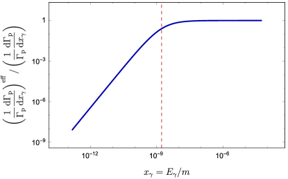
(a)

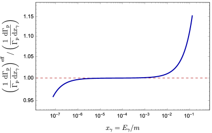
(b)

Figure 4: Log-log plot of the ratio of the effective theory amplitude to the tree level electroweak amplitude for $\text{p-Ps}\to\gamma\nu\bar{\nu}$ decays in LABEL:sub@fig:pRatio1 the low-energy limit $\alpha^{6}<x_{\gamma}<\alpha^{2}$ and LABEL:sub@fig:pRatio2 the high-energy limit $\alpha^{3}/5<x_{\gamma}<1$. The vertical line in LABEL:sub@fig:pRatio1 indicates the hyperfine splitting energy ($x_{\gamma}=\epsilon=7\alpha^{4}/12$) while the horizontal line in LABEL:sub@fig:pRatio2 is placed at 1 to indicate the region where the effective and full theory spectra are equal.

V.4 Soft Photon Spectrum for $\boldsymbol{\text{o-Ps}\to\gamma\nu\bar{\nu}}$

In $\text{o-Ps}\to\gamma\nu_{\ell}\bar{\nu}_{\ell}$ decays, the E1 transition takes the initial o-Ps ground state, $1^{3}S_{1}$, to the excited o-Ps states $n^{3}P_{0,1,2}$ ($n\neq 1$), which then decay into a $\nu_{\ell}\bar{\nu}_{\ell}$ pair. The M1 transition takes the initial o-Ps state, $1^{3}S_{1}$, to the p-Ps ground state, $1^{1}S_{0}$, which cannot decay into a $\nu_{\ell}\bar{\nu}_{\ell}$ pair and therefore does not need to be considered.

The effective theory $\text{o-Ps}\to\gamma\nu_{\ell}\bar{\nu}_{\ell}$ decay amplitude, Fig. LABEL:sub@fig:o-Ps_soft_gnn, is given by

$$\mathcal{M}_{\text{o}}^{\text{eff}} = \sum_{n}\frac{i\langle 0|\hat{A}^{\left(\nu_{\ell}\bar{\nu}_{\ell}\right)}_{\text{p}}|n\rangle\langle n|ie\mathbf{x}\cdot\mathbf{E}|\text{o-Ps}\rangle}{E_{o}-E_{n}-E_{\gamma}}$$ (47)

$$= -2\sqrt{2}i\text{G}_{\text{F}}ea_{\ell}E_{\gamma}\sum_{n}\frac{\langle 0|\left(\mathbf{J}\times\boldsymbol{\sigma}\right)\cdot\mathbf{p}|n\rangle\langle n|\mathbf{x}\cdot\boldsymbol{\epsilon}_{\gamma}|\text{o-Ps}\rangle}{E_{\text{o}}-E_{n}-E_{\gamma}},$$

where $\hat{A}^{\left(\nu_{\ell}\bar{\nu}_{\ell}\right)}_{\text{p}}$ is the p-wave $\text{o-Ps}\to\nu_{\ell}\bar{\nu}_{\ell}$ annihilation operator (derived in Appendix C),

$$\hat{A}^{\left(\nu_{\ell}\bar{\nu}_{\ell}\right)}_{\text{p}}=-2\sqrt{2}\text{G}_{\text{F}}a_{\ell}\left(\mathbf{J}\times\boldsymbol{\sigma}\right)\cdot\mathbf{p}.$$ (48)

As in the calculation of the effective theory $\text{p-Ps}\to\gamma\nu_{\ell}\bar{\nu}_{\ell}$ amplitude (Sec. V.3), we now demonstrate that the effective theory amplitude (without binding) is equal to the soft photon limit of the electroweak amplitude. To calculate the effective theory amplitude, ignoring binding effects, we take $E_{\gamma}\gg m\alpha^{2}$ and ignore $E_{\text{o}}-E_{n}$ in the energy denominator of (47) which yields

$$\mathcal{M}_{\text{o}}^{\text{eff}} \to 2\sqrt{2}i\text{G}_{\text{F}}a_{\ell}e\sum_{n}\langle 0|\left(\mathbf{J}\times\boldsymbol{\sigma}\right)\cdot\mathbf{p}|n\rangle\langle n|\mathbf{x}\cdot\boldsymbol{\epsilon}_{\gamma}|\text{o-Ps}\rangle$$ (49)

$$= 2\sqrt{2}i\text{G}_{\text{F}}a_{\ell}e\langle 0|\left(\mathbf{J}\times\boldsymbol{\sigma}\right)\cdot\mathbf{p}\mathbf{x}\cdot\boldsymbol{\epsilon}_{\gamma}|\text{o-Ps}\rangle.$$

The tensor operator $\mathbf{p}^{i}\mathbf{x}^{j}$ can be decomposed into irreducible spherical tensor operators

$$\mathbf{p}^{i}\mathbf{x}^{j} = \frac{\delta^{ij}}{3}\mathbf{p}\cdot\mathbf{x}+\frac{\mathbf{p}^{i}\mathbf{x}^{j}-\mathbf{p}^{j}\mathbf{x}^{i}}{2}+\frac{1}{2}\left(\mathbf{p}^{i}\mathbf{x}^{j}+\mathbf{p}^{j}\mathbf{x}^{i}-\frac{2}{3}\delta^{ij}\mathbf{p}\cdot\mathbf{x}\right).$$ (50)

Since the initial o-Ps state is an s-wave, only the operator with zero angular momentum (first term of (50)) gives a non-zero matrix element. Additionally, we may take the operator $\mathbf{p}$ to act only on $\mathbf{x}$ because $\mathbf{x}\cdot\boldsymbol{\nabla}\psi_{0}$ vanishes at the origin. With these considerations, the effective theory amplitude (ignoring binding effects) (49) simplifies to

$$\mathcal{M}_{\text{o}}^{\text{eff}}\to 4\text{G}_{\text{F}}ea_{\ell}\left(\mathbf{J}\times\boldsymbol{\epsilon}_{\gamma}\right)\cdot\boldsymbol{\xi}\;\psi_{0}(0).$$ (51)

Since this is equal to the soft photon limit of the tree level electroweak amplitude (33), the E1 transition and annihilation operator (48) fully account for the emitted soft photon and $\nu_{\ell}\bar{\nu}_{\ell}$ annihilation in $\text{o-Ps}\to\gamma\nu_{\ell}\bar{\nu}_{\ell}$ decays. Thus, equation (47) is the complete effective theory amplitude.

We now return to the general case, without any assumptions about photon energies. Expanding the inner products of the effective theory amplitude (47), we find

$$\mathcal{M}_{\text{o}}^{\text{eff}} = 4\text{G}_{\text{F}}ea_{\ell}E_{\gamma}\left(\mathbf{J}\times\boldsymbol{\xi}\right)^{i}\boldsymbol{\epsilon}_{\gamma}^{j}\int\text{d}^{3}x~{}\text{d}^{3}y~{}\delta^{(3)}(\mathbf{x})~{}\partial^{i}_{x}\left(\sum_{n}\frac{\langle\boldsymbol{x}|n\rangle\langle n|\boldsymbol{y}\rangle}{E_{n}+\kappa^{2}/m}\right)y^{j}\psi_{0}(y)$$ (52)

$$= 4\text{G}_{\text{F}}ea_{\ell}E_{\gamma}\left(\mathbf{J}\times\boldsymbol{\xi}\right)^{i}\boldsymbol{\epsilon}_{\gamma}^{j}\int\text{d}^{3}y~{}\left[\partial^{i}_{x}G_{C}(\mathbf{x},\mathbf{y},\kappa)\right]_{\mathbf{x}=\mathbf{0}}y^{j}\psi_{0}(y)$$

where $-\kappa^{2}/m=E_{\text{o}}-E_{\gamma}$ and $G_{C}(\mathbf{x},\mathbf{y},\kappa)$ is the Coulomb Green’s function. The derivative selects the $l=1$ partial wave of the Green’s function Ruiz-Femenia (2008)

$$\left[\partial^{i}_{x}G_{C}(\mathbf{x},\mathbf{y},\kappa)\right]_{\mathbf{x}=\mathbf{0}}=3y^{i}G_{1}(0,y,\kappa).$$ (53)

where the partial wave decomposition of the Coulomb Green’s function can be found in Appendix C of Ref. Manohar and Ruiz-Femenia (2004). Substituting (53) into (52) and preforming the angular integrations yields the effective theory amplitude

$$\mathcal{M}_{\text{o}}^{\text{eff}} = 4\text{G}_{\text{F}}ea_{\ell}\left(\mathbf{J}\times\boldsymbol{\xi}\right)\cdot\boldsymbol{\epsilon}_{\gamma}\psi_{0}(0)\mathcal{A}_{e}(E_{\gamma}).$$ (54)

Here, the electric amplitude, $\mathcal{A}_{\text{e}}$, is determined to be

$$\mathcal{A}_{\text{e}}\left(E_{\gamma}\right) = \frac{4\pi E_{\gamma}}{\psi_{0}(0)}\int_{0}^{\infty}\text{d}y\,y^{4}G_{C,1}\left(0,y;\kappa\right)\psi_{0}(y)$$ (55)

$$= \frac{\left(1-\nu\right)\left(3+5\nu\right)}{3\left(1+\nu\right)^{2}}+\frac{8\nu^{2}\left(1-\nu\right)}{3\left(2-\nu\right)\left(1+\nu\right)^{3}}\;_{2}F_{1}\left(1,2-\nu;3-\nu;\frac{\nu-1}{\nu+1}\right),$$

where $\nu=\frac{\alpha}{\sqrt{4x_{\gamma}+\alpha^{2}}}$. In the first line of (55) we use the integral representation of the electric amplitude from Ref. Voloshin (2004). The hypergeometric function ${}_{2}F_{1}$ simplifies to the so-called Hurwitz-Lerch $\Phi$ function Olver et al. (2011),

$$\frac{1}{2-\nu}\,{{}_{2}F_{1}}\left(1,2-\nu;3-\nu;\frac{\nu-1}{\nu+1}\right) = \frac{1}{2-\nu}\Phi\left(\frac{\nu-1}{\nu+1},1,2-\nu\right)=\sum_{n=0}^{\infty}\frac{1}{2-\nu+n}\left(\frac{\nu-1}{\nu+1}\right)^{n},$$ (56)

$$\mathcal{A}_{\text{e}}\left(E_{\gamma}\right) = \frac{1-\nu}{3\left(1+\nu\right)^{2}}\left[3+5\nu+\frac{8\nu^{2}}{1+\nu}\sum_{n=0}^{\infty}\frac{1}{2-\nu+n}\left(\frac{\nu-1}{\nu+1}\right)^{n}\right].$$ (57)

At high energies, equivalent to $x_{\gamma}\gg\alpha^{2}$ and $\nu\simeq\frac{\alpha}{2\sqrt{x_{\gamma}}}\to 0$, this amplitude can be expanded as a series in $\alpha/\sqrt{x_{\gamma}}$,

$$\mathcal{A}_{\text{e}}=1-\frac{2\alpha}{3\sqrt{x_{\gamma}}}+\frac{\left(2-2\ln 2\right)\alpha^{2}}{3x_{\gamma}}+\dots,\quad(x_{\gamma}\gg\alpha^{2}).$$ (58)

For $x_{\gamma}\gg\alpha^{2}$, the electric amplitude is thus approximately $1$. In this region the binding effects are relatively unimportant. Indeed, the expression (54) agrees with the amplitude obtained when binding effects are ignored, eq. (51), when we take $\mathcal{A}_{e}\to 1$.

On the other hand, in the extreme soft photon limit $x_{\gamma}\ll\alpha^{2}$, equivalent to $\nu\simeq 1-\frac{2x_{\gamma}}{\alpha^{2}}\to 1^{-}$, the electric amplitude can be expanded as a series in $x_{\gamma}/\alpha^{2}$. The leading behaviour is

$$\mathcal{A}_{\text{e}}=\frac{2x_{\gamma}}{\alpha^{2}}+\dots\quad(x_{\gamma}\ll\alpha^{2}).$$ (59)

The leading term in the soft photon limit is linear in $x_{\gamma}$ with a slope of $2/\alpha^{2}$.

To summarize, the electric amplitude is linear in the photon energy below the binding energy and approximately constant above it. The expansions (59) and (58) will be important when determining the behaviour of the photon spectrum in the limits $x_{\gamma}\ll\alpha^{2}$ and $x_{\gamma}\gg\alpha^{2}$.

It is instructive to look for a simpler way to derive the leading low-energy term (59). In the soft photon limit, the wavelength is large and the electric field of the wave is approximately constant. This is similar to the situation in the Stark effect. Since the first order correction to the ground state energy for the Stark effect vanishes ($E^{(1)}\propto\langle\psi_{0}|\mathbf{x}\cdot\boldsymbol{\epsilon}_{\gamma}|\psi_{0}\rangle=0$), one evaluates the second order correction to the ground state energy

$$E^{(2)}=\sum_{n\neq 0}\frac{\langle\psi_{0}|H^{\prime}|n\rangle\langle n|H^{\prime}|\psi_{0}\rangle}{E_{0}-E_{n}},$$ (60)

where $H^{\prime}\propto\mathbf{x}\cdot\boldsymbol{\epsilon}_{\gamma}=r\cos\theta$. The form of (60) is similar to the low-energy limit of the effective theory amplitude where $E_{\gamma}=0$ in the energy denominator of (47)

$$\mathcal{M}_{\text{o}}^{\text{eff}} = -2\sqrt{2}i\text{G}_{\text{F}}ea_{\ell}E_{\gamma}\sum_{n}\frac{\langle 0|\left(\mathbf{J}\times\boldsymbol{\sigma}\right)\cdot\mathbf{p}|n\rangle\langle n|\mathbf{x}\cdot\boldsymbol{\epsilon}_{\gamma}|\text{o-Ps}\rangle}{E_{\text{o}}-E_{n}}.$$ (61)

Since equation (60) can be summed exactly using the method of Dalgarno and Lewis Dalgarno and Lewis (1955); Schwartz (1959), we can exploit the similarity between equations (60) and (61) to evaluate the effective theory amplitude in the soft photon limit.

Equations (60) and (61) can be summed exactly by finding a function $F$ that satisfies

$$[F,H_{0}]\psi_{0}(\mathbf{x})=\mathbf{x}\cdot\boldsymbol{\epsilon}_{\gamma}\psi_{0}(\mathbf{x}).$$ (62)

For the unperturbed positronium Hamiltonian, $H_{0}$, the function $F$ is given by

$$F=-\frac{m}{2}\mathbf{x}\cdot\boldsymbol{\epsilon}_{\gamma}\left(a^{2}+\frac{ar}{2}\right).$$ (63)

With $F$ in hand, we evaluate equation (61)

$$\mathcal{M}_{\text{o}}^{\text{eff}} = -2\sqrt{2}i\text{G}_{\text{F}}ea_{\ell}E_{\gamma}\langle 0|\left(\mathbf{J}\times\boldsymbol{\sigma}\right)\cdot\mathbf{p}F|\text{o-Ps}\rangle$$ (64)

$$= -4\text{G}_{\text{F}}ea_{\ell}E_{\gamma}\left(\mathbf{J}\times\boldsymbol{\xi}\right)\cdot\int\text{d}^{3}x\;\delta^{(3)}(\mathbf{x})\boldsymbol{\nabla}(F\psi_{0}(\mathbf{x}))$$

$$= 4\text{G}_{\text{F}}ea_{\ell}\psi_{0}(0)\left(\boldsymbol{\epsilon}_{\gamma}\times\mathbf{J}\right)\cdot\boldsymbol{\xi}\frac{2x_{\gamma}}{\alpha^{2}}.$$

Thus, in the limit $x_{\gamma}\ll\alpha^{2}$ the electric amplitude is $\mathcal{A}_{e}\approx 2x_{\gamma}/\alpha^{2}$ which is equal to the first order term of the expansion (59).

Similarly, the Stark effect can be related to the soft photon limit of the E1 portion of the $\text{o-Ps}\to 3\gamma$ decay amplitude. The annihilation operator that contributes to the E1 portion of the $\text{o-Ps}\to 3\gamma$ decay amplitude is of the same form as the o-Ps p-wave $\nu_{\ell}\bar{\nu}_{\ell}$ annihilation operator and contains a $\mathbf{p}$ derivitive. A calculation, using the summation technique above, reveals that in the soft photon limit, $\mathcal{A}_{e}\approx 2x_{\gamma}/\alpha^{2}$. This agrees with the soft photon limit of the electric amplitude derived in Manohar and Ruiz-Femenia (2004); Ruiz-Femenia (2008) by expansion of the p-wave Green’s function.

With this understanding of the electric amplitude, we proceed to the photon spectrum. Both the spin averaged square of the amplitude (54) and the three body phase space in the $x\to 0$ limit are needed. Squaring (54), summing over the photon polarizations and averaging over the initial o-Ps polarizations, yields

$$\frac{1}{3}\sum_{\boldsymbol{\xi}\boldsymbol{\epsilon}_{\gamma}}\left|\mathcal{M}_{\text{o}}^{\text{eff}}\right|^{2} = \frac{1}{3}\sum_{\boldsymbol{\xi}\boldsymbol{\epsilon}_{\gamma}}\left|4\text{G}_{\text{F}}ea_{\ell}\psi_{0}(0)\mathcal{A}_{\text{e}}(E_{\gamma})\left(\boldsymbol{\epsilon}_{\gamma}\times\mathbf{J}\right)\cdot\boldsymbol{\xi}\right|^{2}$$ (65)

$${}_{x_{\gamma}\to 0}\to 128\text{G}_{\text{F}}^{2}a_{\ell}^{2}\alpha^{4}m^{5}\left|\mathcal{A}_{\text{e}}(E_{\gamma})\right|^{2}\left(1-\frac{1}{3}\cos^{2}\theta\right),$$

where $\sum_{\boldsymbol{\xi}\boldsymbol{\epsilon}_{\gamma}}|\left(\boldsymbol{\epsilon}_{\gamma}\times\mathbf{J}\right)\cdot\boldsymbol{\xi}|^{2}/3=(16E_{1}^{2})(1-\frac{1}{3}(\hat{\mathbf{k}}_{\gamma}\cdot\hat{\mathbf{k}}_{1})^{2})$, $\hat{\mathbf{k}}_{\gamma}\cdot\hat{\mathbf{k}}_{1}=\cos\theta$ and $E_{1}\to m$. Multiplying by the three body phase space in the limit $x_{\gamma}\to 0$ and integrating over $\cos\theta$ yields the effective theory spectrum

$$\left(\frac{1}{\Gamma_{\text{o}}}\frac{\text{d}\Gamma_{\text{o}}}{\text{d}x_{\gamma}}\right)^{\text{eff}} = \frac{27\pi^{3}}{8\text{G}_{\text{F}}^{2}m^{5}\alpha^{4}a_{\ell}^{2}}\int_{-1}^{1}\text{d}\cos\theta\frac{1}{128\pi^{3}}\frac{x_{\gamma}}{2}\frac{1}{3}\sum_{\boldsymbol{\xi}\boldsymbol{\epsilon}_{\gamma}}\left|\mathcal{M}_{\text{o}}^{\text{eff}}(E_{\gamma})\right|^{2}$$ (66)

$$= 3x_{\gamma}\left|\mathcal{A}_{\text{e}}(E_{\gamma})\right|^{2}.$$

The effective theory spectrum is proportional to the square of the electric amplitude and thus shares the same transitional behaviour at $x_{\gamma}=\alpha^{2}$. Substituting the leading term from equations (59) and (58) into (66) we obtain the approximate form of the spectrum in the limits $x_{\gamma}\ll\alpha^{2}$ and $x_{\gamma}\gg\alpha^{2}$

$$\left(\frac{1}{\Gamma_{\text{o}}}\frac{\text{d}\Gamma_{\text{o}}}{\text{d}x_{\gamma}}\right)^{\text{eff}}\approx\begin{cases}\frac{12}{\alpha^{2}}x_{\gamma}^{3}&\text{for }x_{\gamma}\ll\alpha^{2}\\ 3x_{\gamma}&\text{for }x_{\gamma}\gg\alpha^{2}.\end{cases}$$ (67)

Clearly, for photons with $x_{\gamma}\ll\alpha^{2}$, the spectrum is cubic in the photon energy as required by Low’s theorem. For photons in the energy range $\alpha^{2}\ll x_{\gamma}\ll 1$, both the effective theory and tree level electroweak spectra are approximately linear with a slope of 3.

The ratio of the effective theory spectrum to the tree level electroweak spectrum for $\text{o-Ps}\to\gamma\nu_{\ell}\bar{\nu}_{\ell}$ decays is plotted in Fig. 5. The effective theory spectrum and tree level electroweak spectrum are approximately equal in the intermediate energy range $x_{\gamma}\sim\mathcal{O}(10^{-2}-10^{-1})$ (Fig. 5). For high energy photons the ratio spikes upward indicating that the effective theory spectrum differs significantly from the tree level electroweak spectrum and is no longer accurate (Fig. LABEL:sub@fig:oRatio2). Below the binding energy, the ratio in the log-log plot is linear with a slope of slope of 2 since the effective theory spectrum is cubic in $x_{\gamma}$ while the tree level electroweak spectrum is linear (Fig. LABEL:sub@fig:oRatio1).

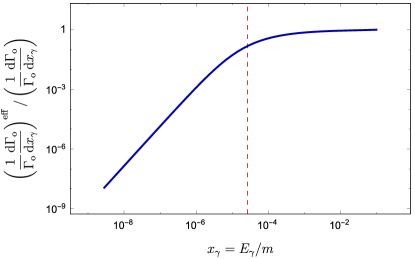
(a)

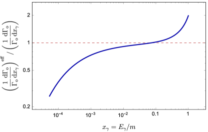
(b)

Figure 5: Log-log plot of the ratio of the effective theory amplitude to the tree level electroweak amplitude for $\text{p-Ps}\to\gamma\nu\bar{\nu}$ decays for LABEL:sub@fig:pRatio1 the low-energy limit $\alpha^{4}<x_{\gamma}<0.1$ and for LABEL:sub@fig:pRatio2 the high-energy limit $\alpha^{2}<x_{\gamma}<1$. The vertical line in LABEL:sub@fig:pRatio1 indicates the binding energy ($x_{\gamma}=\alpha^{2}/2$) while the horizontal line in LABEL:sub@fig:pRatio2 is placed at 1 where the effective theory and electroweak theory spectra are equal.

VI Conclusions

We calculated the decay rate and photon spectrum of the decay of Ps into a photon and a neutrino-antineutrino pair ($\text{Ps}\to\gamma\nu_{\ell}\bar{\nu}_{\ell}$). Both Ps spin states have access to the $\gamma\nu_{\ell}\bar{\nu}_{\ell}$ decay channel where the p-Ps and o-Ps final states are orthogonal despite being comprised of the same particles. The decay rates are given by (4) and (5) and the tree level electroweak photon spectrum by (9) and (10). These rates and spectra were further examined by calculating the angular dependence of the decay amplitudes, angular distributions and spectra for specific $\gamma+Z^{*}$ final states (Tables 1–4).

In principle, this decay could be observed. Experimentally, this channel would appear as the decay of Ps into a single photon if the neutrinos go undetected. Experimental detection of this channel would however be very challenging given the small branching ratios.

The soft photon limit of the tree level electroweak spectra (equations (9) and (10)) was compared with that predicted by Low’s theorem and found to be in disagreement. This contradiction was resolved by including binding effects in the computation of the soft photon spectrum using the methods of non-relativistic effective field theories. The effective theory spectra are given by equations (45) and (66), and are valid for photon energies much less than the electron mass.

For photon energies much larger than the hyperfine splitting yet still much smaller than the electron rest mass ($m\alpha^{4}\ll E_{\gamma}\ll m$), the $\text{p-Ps}\to\gamma\nu_{\ell}\bar{\nu}_{\ell}$ effective theory spectrum approaches the tree level electroweak spectrum (9). Below the hyperfine splitting ($E_{\gamma}\ll m\alpha^{4}$), the effective theory spectrum is cubic in the soft photon energy as required by Low’s theorem. In the dipole approximation of the Coulomb interaction, soft photon $\text{p-Ps}\to\gamma\nu_{\ell}\bar{\nu}_{\ell}$ decays proceed only by the magnetic M1 transition.

The $\text{o-Ps}\to\gamma\nu_{\ell}\bar{\nu}_{\ell}$ effective theory spectrum approaches the tree level electroweak spectrum (10) for photon energies much larger than the binding energy but still much smaller than the electron rest mass($m\alpha^{2}\ll E_{\gamma}\ll m$). For photon energies much smaller than the binding energy ($E_{\gamma}\ll m\alpha^{2}$), the effective theory spectrum is cubic in the photon energy as required by Low’s theorem. In the dipole approximation of the Coulomb interaction, soft photon $\text{o-Ps}\to\gamma\nu_{\ell}\bar{\nu}_{\ell}$ decays proceed only by the electric E1 transition.

Lastly, we find connection between the Stark effect and the soft photon limit of the $\text{o-Ps}\to\gamma\nu_{\ell}\bar{\nu}_{\ell}$ spectrum and the E1 contribution to the $\text{o-Ps}\to 3\gamma$ spectrum.

Appendix A: Formulation of the $\boldsymbol{\text{Ps}\to\gamma\nu_{\ell}\bar{\nu}_{\ell}}$ decay rate in terms of $\boldsymbol{\gamma}$ and $\boldsymbol{Z^{*}}$

The Feynman diagrams relevant for the $\text{Ps}\to\gamma\nu_{\ell}\bar{\nu}_{\ell}$ decay are illustrated in Fig. 1. As in Sec. II we neglect the 3-momentum of the incoming leptons and the virtual $W$ and $Z$ bosons. With these approximations, the $(\text{p/o})\text{-}\text{Ps}\to\gamma\nu_{\ell}\bar{\nu}_{\ell}$ amplitudes are

$$i\mathcal{M}_{\text{p/o}} = \frac{i\text{G}_{\text{F}}}{\sqrt{2\pi\alpha}}(\epsilon_{\gamma})^{*}_{\mu}g_{\nu\rho}\text{Tr}\left[X_{\text{p/o}}^{\mu\nu}(p_{1},k_{\gamma})\right]J^{\rho}(k_{1},k_{2}),$$ (68)

where

$$X_{\text{p/o}}^{\mu\nu}(p_{1},k_{\gamma}) = \text{Tr}\left[2m\Psi_{\text{p/o}}\left((ie)\gamma^{\nu}\left(b_{\ell}-a_{\ell}\gamma^{5}\right)\frac{\cancel{p}_{1}-\cancel{k}_{\gamma}+m}{(p_{1}-k_{\gamma})^{2}-m^{2}}(-ie)\gamma^{\mu}\right.\right.$$ (69)

$$\;\;\;\;\;\;\;\;\;\;\;\;\;\;\left.\left.+(-ie)\gamma^{\mu}\frac{\cancel{k}_{\gamma}-\cancel{p}_{2}+m}{(k_{\gamma}-p_{2})^{2}-m^{2}}(ie)\gamma^{\nu}\left(b_{\ell}-a_{\ell}\gamma^{5}\right)\right)\right],$$

and $J^{\mu}\left(k_{1},k_{2}\right)=\bar{u}(k_{1})\gamma^{\mu}\left(1-\gamma^{5}\right)v(k_{2})$ is the neutral weak current. The p-Ps and o-Ps projection operators are given by $\Psi_{\text{p}}=\left(1+\gamma^{0}\right)\gamma^{5}/(2\sqrt{2})$ and $\Psi_{\text{o}}=\left(1+\gamma^{0}\right)\boldsymbol{\gamma}\cdot\boldsymbol{\xi}/(2\sqrt{2})$ where $\boldsymbol{\xi}$ is the o-Ps polarization vector Czarnecki et al. (1999b).

To calculate the $\text{Ps}\to\gamma\nu_{\ell}\bar{\nu}_{\ell}$ decay rate, we start from the standard formula,

$$\Gamma_{\text{p/o}} = \frac{1}{2m_{\text{Ps}}}\int\text{d}\Phi_{3}(p_{1}+p_{2};k_{1},k_{2},k_{\gamma})\frac{\left|\psi_{\text{0}}(0)\right|^{2}}{m}\frac{1}{g}\sum_{\text{spin/pol}}\left|\mathcal{M}_{\text{p/o}}\right|^{2},$$ (70)

where $\psi_{\text{0}}(0)$ is the ground state positronium wave function at the origin and $g$ is the number of Ps polarizations of the initial state Peskin and Schroeder (1997).

Substituting the three-body spin averaged matrix element squared

$$\sum_{\text{spin/pol}}\left|\mathcal{M}_{\text{p/o}}\right|^{2} = g_{\alpha\beta}g_{\mu\rho}g_{\nu\sigma}\frac{\text{G}_{\text{F}}^{2}}{2\pi\alpha}X_{\text{p/o}}^{\alpha\mu}{X_{\text{p/o}}^{\beta\nu}}^{*}\text{Tr}\left[\cancel{k}_{1}\gamma^{\rho}(1-\gamma^{5})\cancel{k}_{2}\gamma^{\sigma}(1-\gamma^{5})\right],$$ (71)

into (70) and decomposing the three-body phase space into two two-body phase spaces, yields

$$\Gamma_{\text{p/o}} = \frac{1}{2m_{\text{Ps}}}\int\frac{\text{d}s}{2\pi}\text{d}\Phi_{2}(2p_{1};k_{\gamma},q)\frac{\left|\psi_{\text{Ps}}(0)\right|^{2}}{m}\frac{g_{\alpha\beta}g_{\mu\rho}g_{\nu\sigma}}{g}\frac{\text{G}_{\text{F}}^{2}}{2\pi\alpha}X_{\text{p/o}}^{\alpha\mu}{X_{\text{p/o}}^{\beta\nu}}^{*}$$ (72)

$$\int\text{d}\Phi_{2}(q;k_{1},k_{2}){k_{1}}_{\eta}{k_{2}}_{\lambda}\text{Tr}\left[\gamma^{\eta}\gamma^{\rho}(1-\gamma^{5})\gamma^{\lambda}\gamma^{\sigma}(1-\gamma^{5})\right],$$

where $s=q\cdot q$ is the invariant mass of $Z^{*}$ squared and $q$ is its four-momentum. The neutrino phase space integral can be performed by writing the neutrino momentum product, ${k_{1}}_{\eta}{k_{2}}_{\lambda}$, as a linear combination of the only available tensors, ${k_{1}}_{\eta}{k_{2}}_{\lambda}=Aq^{2}g_{\eta\lambda}+Bq_{\eta}q_{\lambda}$. The momentum conserving delta function in $\text{d}\Phi_{2}(q;k_{1},k_{2})$ forces $q=k_{1}+k_{2}$. A system of equations for $A$ and $B$ is obtained by contracting $\int\text{d}\Phi_{2}(q;k_{1},k_{2}){k_{1}}_{\eta}{k_{2}}_{\lambda}$ with $g^{\eta\lambda}$ and $q^{\eta}q^{\lambda}$, and yields the solution $A=1/12$ and $B=1/6$. Thus, the neutrino contribution to the decay rate is

$$\int\text{d}\Phi_{2}(q;k_{1},k_{2}){k_{1}}_{\eta}{k_{2}}_{\lambda}\text{Tr}\left[\gamma^{\eta}\gamma^{\rho}(1-\gamma^{5})\gamma^{\lambda}\gamma^{\sigma}(1-\gamma^{5})\right] = \frac{1}{3\pi}\left[q^{\rho}q^{\sigma}-q^{2}g^{\rho\sigma}\right]$$ (73)

$$= \frac{1}{3\pi}q^{2}\sum_{s}\epsilon_{s}^{\rho}(q){\epsilon_{s}^{\sigma}}^{*}(q),$$

where the sum over the polarizations of a massive vector boson is given by

$$\sum_{s}\epsilon_{s}^{\rho}(q){\epsilon_{s}^{\sigma}}^{*}(q)=\frac{q^{\rho}q^{\sigma}}{q^{2}}-g^{\rho\sigma}.$$ (74)

Substituting (73) into equation (72), we obtain the $\text{Ps}\to\gamma\nu_{\ell}\bar{\nu}_{\ell}$ decay rate in terms of $\text{Ps}\rightarrow\gamma Z^{*}$

$$\Gamma_{\text{p/o}} = \frac{1}{2m_{\text{Ps}}}\int\frac{\text{d}s}{2\pi}\text{d}\Phi_{2}(2p_{1};k_{\gamma},q)\frac{\left|\psi_{Ps}(0)\right|^{2}}{m}\frac{g_{\alpha\beta}}{g}\frac{\text{G}_{\text{F}}^{2}}{2\pi\alpha}X_{\text{p/o}}^{\alpha\mu}{X_{\text{p/o}}^{\beta\nu}}^{*}\frac{1}{3\pi}q^{2}\sum_{s}\left(\epsilon_{s}\right)_{\mu}\left(\epsilon_{s}^{*}\right)_{\nu}$$ (75)

$$= \frac{\text{G}_{\text{F}}^{2}}{2\pi^{2}\alpha}\int\frac{\text{d}q^{2}}{2\pi}q^{2}\left(\frac{1}{2m_{\text{Ps}}}\int\text{d}\Phi_{2}(2p;k_{\gamma},q)\frac{\left|\psi_{Ps}(0)\right|^{2}}{m}\frac{1}{3g}\sum_{\text{pol}}\left|\mathcal{M}_{\text{(p/o)-Ps}\to\gamma Z^{*}}\right|^{2}\right)$$

$$= \frac{\text{G}_{\text{F}}^{2}}{2\pi^{2}\alpha}\int\frac{\text{d}q^{2}}{2\pi}q^{2}\Gamma_{\text{(p/o)-Ps}\to\gamma Z^{*}}.$$

Appendix B: Derivation of the o-Ps amplitudes with their angular dependencies

Initially, the o-Ps atom is in a state of definite angular momentum denoted by $|\Lambda\rangle$. Since o-Ps and its decay products, $\gamma$ and $Z^{*}$, are all spin one particles, we abbreviate the angular momentum states $|1,m_{s}\rangle$ by $|m_{s}\rangle$ where $m_{s}$ is the projection of spin along the $z$-axis. The massive $Z^{*}$ boson has access to all three spin projection states (i.e., $m_{Z}\in\{\pm 1,0\}$) while the massless photon cannot access the longitudinally polarized $|0\rangle$ state (i.e., $m_{\gamma}\in\{\pm 1\}$). Conservation of angular momentum requires that the spin projection quantum numbers satisfy $m_{\gamma}+m_{Z}=m_{\Lambda}$; as a result, there are four different modes in which o-Ps can decay along the $z$-axis.

Consider $|\Lambda\rangle$ initially polarized in the state $|+\rangle$ along the $z$-axis. Since the photon must have $m_{\gamma}=\pm 1$, conservation of angular momentum implies $|\gamma\rangle=|+\rangle$ and $|Z^{*}\rangle=|0\rangle$; we assign the amplitude $A_{+0}$ to this decay. If $|\Lambda\rangle$ is initially polarized in the state $|-\rangle$, $|\gamma\rangle=|-\rangle$ and $|Z^{*}\rangle=|0\rangle$; we assign the amplitude $A_{-0}$ to this decay. Lastly, if $|\Lambda\rangle$ is initially polarized in the state $|0\rangle$, $m_{\gamma}=-m_{Z}$ and therefore $|\gamma\rangle=|\pm\rangle$ and $|Z^{*}\rangle=|\mp\rangle$; we assign amplitudes $A_{\pm\mp}$ to these decays.

The $\text{o-Ps}\to\gamma Z^{*}$ amplitudes along the $z$-axis are

$$A_{\pm 0} = \pm\frac{4e^{2}a_{\ell}}{q}\left[\frac{E_{\gamma}+E_{Z}}{q}\boldsymbol{\xi}\cdot\boldsymbol{\epsilon}_{\pm}^{*}\right]=\pm\frac{e^{2}}{\sqrt{2}}\frac{E_{\gamma}+E_{Z}}{q}\delta_{m_{\Lambda},\pm},$$ (76)

$$A_{\pm\mp} = \pm\frac{4ie^{2}a_{\ell}}{\sqrt{2}}\boldsymbol{\xi}\cdot\hat{{\bf z}}=\pm\frac{ie^{2}}{\sqrt{2}}\delta_{m_{\Lambda},0},$$ (77)

where $\boldsymbol{\epsilon}_{\pm}$ are the transverse polarization vectors of the photon and $\boldsymbol{\xi}$ is the o-Ps polarization vector. Here $q$ is the momentum of the $Z^{*}$.

To determine the angular dependence of the decay amplitudes on the spherical angles, $\theta$ and $\phi$, we consider two coordinate systems $\{x,y,z\}$ and $\{x^{\prime},y^{\prime},z^{\prime}\}$. The $z^{\prime}$-axis is defined by the angles $\theta$ and $\phi$ in the $\{x,y,z\}$ coordinate system and represents the decay axis. The angular dependence of the decay amplitudes is constructed by rotating the initial o-Ps state and then considering the decay into $\gamma+Z^{*}$ along $z^{\prime}$.

The combination of rotations required to bring $\{x,y,z\}$ onto $\{x^{\prime},y^{\prime},z^{\prime}\}$ (Fig. 6) is determined to be

$$R=R_{z^{\prime}}(\alpha)R_{y^{\prime}}(\theta)R_{z^{\prime}}(\phi),$$ (78)

where $R_{{\bf n}}(\theta)=e^{i\theta{\bf n}\cdot{\bf S}}$ is the operator for rotations about the axis given by the unit vector, $\mathbf{n}$, and ${\bf S}=(S_{x},S_{y},S_{z})$ is the spin-one matrix operator Dick (2016).

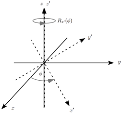
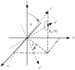
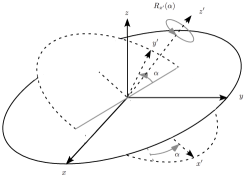
Figure 6: Sequence of rotations that transforms $\{x,y,z\}$ (solid) to $\{x^{\prime},y^{\prime},z^{\prime}\}$ (dashed).

Application of $R$ to $|\Lambda\rangle$ yields the amplitude for $|\Lambda\rangle$ to be in the state $|m_{\Lambda}^{\prime}\rangle$ along the $z^{\prime}$-axis for each $m_{\Lambda}^{\prime}\in\{\pm 1,0\}$. If $|\Lambda\rangle$ is initially polarized in the state $|+\rangle$, then $|\Lambda\rangle$ has an amplitude of $\frac{1}{2}(1+\cos\theta)e^{i\alpha}e^{i\phi}$ to be in the state $|+^{\prime}\rangle$ (the $m_{\Lambda}=1$ state along the $z^{\prime}$ axis). If $|\Lambda\rangle$ is in the state $|+^{\prime}\rangle$, it decays to $|+^{\prime};k\hat{\mathbf{z}}^{\prime}\rangle_{\gamma}\otimes|0^{\prime};-k\hat{\mathbf{z}}^{\prime}\rangle_{Z}$ with an amplitude $A_{+^{\prime}0^{\prime}}$, where $k$ is the magnitude of the photon momentum along $z^{\prime}$. Thus, the total amplitude for the decay of an o-Ps atom with spin projection $m_{\Lambda}=+1$ into a photon moving along $+z^{\prime}$-axis with spin projection $m^{\prime}_{\gamma}=+1$ is

$$\mathcal{A}^{m_{\Lambda}=+}_{+^{\prime}0^{\prime}}\left(\theta,\phi\right)=\frac{A_{+^{\prime}0^{\prime}}}{2}(1+\cos\theta)e^{i\alpha}e^{i\phi}.$$ (79)

Similarly, the amplitude for the final state $|-^{\prime};k\hat{\mathbf{z}}^{\prime}\rangle_{\gamma}\otimes|0^{\prime};-k\hat{\mathbf{z}}^{\prime}\rangle_{Z}$ is

$$\mathcal{A}^{+}_{-^{\prime}0^{\prime}}\left(\theta,\phi\right)=\frac{A_{-^{\prime}0^{\prime}}}{2}(1-\cos\theta)e^{-i\alpha}e^{i\phi},$$ (80)

and the amplitudes for $|\pm^{\prime};k\hat{\mathbf{z}}^{\prime}\rangle_{\gamma}\otimes|\mp^{\prime};-k\hat{\mathbf{z}}^{\prime}\rangle_{Z}$ are

$$\mathcal{A}^{+}_{\pm^{\prime}\mp^{\prime}}\left(\theta,\phi\right)=\frac{-A_{\pm^{\prime}\mp^{\prime}}}{\sqrt{2}}\sin\theta e^{i\phi}.$$ (81)

We denote the o-Ps decay amplitudes with their full angular dependencies as $\mathcal{A}_{m_{\gamma}^{\prime}m_{Z}^{\prime}}^{m_{\Lambda}}$ where $m_{\Lambda}\in\{\pm 1,0\}$ is the initial spin projection of o-Ps along the $z$-axis, and, $m_{\gamma}^{\prime}\in\{\pm 1\}$ and $m_{Z}^{\prime}\in\{\pm 1,0\}$ are the spin projections of the photon and $Z^{*}$ along the $z^{\prime}$-axis. The amplitudes, $\mathcal{A}^{0}_{m_{\gamma}^{\prime}m_{Z}^{\prime}}$, are obtained using the method outlined above while $\mathcal{A}^{-}_{m_{\gamma}^{\prime}m_{Z}^{\prime}}$ is obtained from $\mathcal{A}^{+}_{m_{\gamma}^{\prime}m_{Z}^{\prime}}$ by the prescription $\theta\rightarrow\theta+\pi$, $\phi\rightarrow-\phi$ and $\alpha\rightarrow-\alpha$. The o-Ps amplitudes, $\mathcal{A}^{m_{\Lambda}}_{m_{\gamma}^{\prime}m_{Z}^{\prime}}$, are listed in table 2 where we have chosen the convention $\alpha=0$.

Appendix C: Derivation of the $\boldsymbol{e^{+}e^{-}\rightarrow\nu\bar{\nu}}$ annihilation operator

(a)

(b)

Figure 7: The $e^{+}e^{-}\rightarrow\nu_{\ell}\bar{\nu}_{\ell}$ annihilation graphs for LABEL:sub@fig:nnZ $Z$ boson exchange and LABEL:sub@fig:nnW $W$ boson exchange. The graph LABEL:sub@fig:nnZ contributes to the $\text{Ps}\to\nu_{\ell}\bar{\nu}_{\ell}$ amplitude for all lepton flavours $\ell=e,\mu,\tau$ while LABEL:sub@fig:nnW only contributes to the amplitude when $\ell=e$.

In order to calculate the effective theory amplitudes (Sec. V), we require the $\mathcal{O}(|\mathbf{p}|/m)$ expansion of the $e^{+}e^{-}\to\nu_{\ell}\bar{\nu}_{\ell}$ annihilation amplitude (Fig. 7). The electron and positron 4-momentum are $p_{1}=(E,\mathbf{p})$ and $p_{2}=(E,-\mathbf{p})$ while the neutrino and anti-neutrino 4-momentum are $k_{1}$ and $k_{2}$. The amplitude of Fig. 7 is

$$A^{(\nu_{\ell}\bar{\nu}_{\ell})} = -i\sqrt{2}\text{G}_{\text{F}}\bar{v}(-\mathbf{p})\cancel{J}(v_{\ell}-a_{\ell}\gamma^{5})u(\mathbf{p})$$ (85)

$$= 2\sqrt{2}i\text{G}_{\text{F}}m\chi^{\dagger}\left[\left(\begin{array}[]{cc}\frac{\left(\boldsymbol{\sigma}\cdot\mathbf{p}\right)^{\dagger}}{2mc}&1\end{array}\right)\cancel{J}\left(v_{\ell}-a_{\ell}\gamma^{5}\right)\left(\begin{array}[]{c}1\\ \frac{\boldsymbol{\sigma}\cdot\mathbf{p}}{2mc}\end{array}\right)\right]\phi$$

$$= \chi^{\dagger}\hat{A}^{(\nu_{\ell}\bar{\nu}_{\ell})}\phi,$$ (86)

where

$$\hat{A}^{(\nu_{\ell}\bar{\nu}_{\ell})} = 2\sqrt{2}i\text{G}_{\text{F}}m\left(\begin{array}[]{cc}\frac{\boldsymbol{\sigma}\cdot\mathbf{p}}{2m}&1\end{array}\right)\left(\begin{array}[]{cc}J_{0}&-\mathbf{J}\cdot\boldsymbol{\sigma}\\ \mathbf{J}\cdot\boldsymbol{\sigma}&-J_{0}\end{array}\right)\left(\begin{array}[]{cc}v_{\ell}&-a_{\ell}\\ -a_{\ell}&v_{\ell}\end{array}\right)\left(\begin{array}[]{c}1\\ \frac{\boldsymbol{\sigma}\cdot\mathbf{p}}{2m}\end{array}\right)$$ (94)

is the $\nu_{\ell}\bar{\nu}_{\ell}$ annihilation operator. From momentum conservation, $\mathbf{k}_{1}=-\mathbf{k}_{2}$ and the time component of the neutral weak current vanishes, $J_{0}=0$. Therefore, the $\nu_{\ell}\bar{\nu}_{\ell}$ annihilation operator becomes

$$\hat{A}^{(\nu_{\ell}\bar{\nu}_{\ell})}=2\sqrt{2}i\text{G}_{\text{F}}mv_{\ell}\left(\mathbf{J}\cdot\boldsymbol{\sigma}\right)-2\sqrt{2}\text{G}_{\text{F}}a_{\ell}\left(\mathbf{J}\times\boldsymbol{\sigma}\right)\cdot\mathbf{p}.$$ (95)

The first term of equation (95), proportional to vector coupling, is the s-wave $\text{o-Ps}\to\nu_{\ell}\bar{\nu}_{\ell}$ annihilation operator

$$\hat{A}^{(\nu_{\ell}\bar{\nu}_{\ell})}_{\text{s}}=2\sqrt{2}i\text{G}_{\text{F}}mv_{\ell}\left(\mathbf{J}\cdot\boldsymbol{\sigma}\right).$$ (96)

In the computation of the $\text{p-Ps}\to\gamma\nu_{\ell}\bar{\nu}_{\ell}$ effective theory amplitude, the s-wave annihilation operator takes the intermediate s-wave o-Ps state into a neutrino-antineutrino pair. The second term, proportional to axial coupling, is the p-wave $\text{o-Ps}\to\nu_{\ell}\bar{\nu}_{\ell}$ annihilation operator

$$\hat{A}^{(\nu_{\ell}\bar{\nu}_{\ell})}_{\text{p}}=-2\sqrt{2}\text{G}_{\text{F}}a_{\ell}\left(\mathbf{J}\times\boldsymbol{\sigma}\right)\cdot\mathbf{p}.$$ (97)

In the computation of the $\text{o-Ps}\to\gamma\nu_{\ell}\bar{\nu}_{\ell}$ effective theory amplitude, the p-wave annihilation operator takes the intermediate p-wave o-Ps states into a neutrino-antineutrino pair.

References

- Pirenne (1947) J. Pirenne, Arch. Sci. Phys. Nat. 29, 207 (1947) .
- Ore and Powell (1949) A. Ore and J. L. Powell, Phys. Rev. 75, 1696 (1949) .
- Kniehl and Penin (2000) B. A. Kniehl, A. V. Kotikov and O. L. Veretin, Phys. Rev. A80, 052501 (2009), arXiv:hep-ph/0004267 .
- Adkins (2015) G. S. Adkins, Hyperfine Interact. 233, (2015) 59-66 .
- Adkins et al. (2003) G. S. Adkins, N. M. McGovern, R. N. Fell, and J. Sapirstein, Phys. Rev. A68, 032512 (2003), arXiv:hep-ph/0305251 .
- Adkins et al. (2001) G. S. Adkins, R. N. Fell, and J. Sapirstein, Phys. Rev. A63, 032511 (2001).
- Adkins et al. (2000) G. S. Adkins, R. N. Fell, and J. Sapirstein, Phys. Rev. Lett. 84, 5086 (2000), arXiv:hep-ph/0003028 .
- Czarnecki et al. (1999a) A. Czarnecki, K. Melnikov, and A. Yelkhovsky, Phys. Rev. Lett. 83, 1135 (1999a), erratum ibid. 85, 2221 (2000), arXiv:hep-ph/9904478 .
- Czarnecki et al. (2000) A. Czarnecki, K. Melnikov, and A. Yelkhovsky, Phys. Rev. A61, 052502 (2000), erratum ibid. 62, 059902 (2000), arXiv:hep-ph/9910488 .
- Penin (2014) A. A. Penin, Proc. Sci. LL2014, (2014) 074 .
- Penin (2004) A. A. Penin, Int. J. Mod. Phys. A19, 3897 (2004), arXiv:hep-ph/0308204 .
- Kniehl and Penin (2000) B. A. Kniehl and A. A. Penin, Phys. Rev. Lett. 85, 1210 (2000), erratum ibid. 85, 3065 (2000), arXiv:hep-ph/0004267 .
- Karshenboim (2005) S. G. Karshenboim, Phys. Rept. 422, 1-63 (2005), arXiv:0909.1431 .
- Hill and Lepage (2000) R.J. Hill and G. P. Lepage, Phys. Rev. D62, 111301 (2000), arXiv:hep-ph/0003277 .
- Melnikov and Yelkhovsky (2000) K. Melnikov and A. Yelkhovsky, Phys. Rev. D62, 116003 (2000), arXiv:hep-ph/0008099 .
- Bernreuther and Nachtmann (1981) W. Bernreuther and O. Nachtmann, Z. Phys. C11, 235 (1981).
- Czarnecki and Karshenboim (2000) A. Czarnecki and S. G. Karshenboim, in Proc. XIV Intl. Workshop on High Energy Physics and Quantum Field Theory (QFTHEP’99, Moscow 1999), edited by B. B. Levchenko and V. I. Savrin (MSU-Press, Moscow, 2000) p. 538, arXiv:hep-ph/9911410.
- Asai (1994) S. Asai, K. Shigekuni, T. Sanuki, T. Sanuki, and S. Orito, Phys. Lett. B323, 90 (1994) .
- Maeno (1995) T. Maeno, M. Fujikawa, J. Kataoka, Y. Nishihara, S. Orito, K. Shigekuni, and Y. Watanabe, Phys. Lett. B351, 574 (1995), arXiv:hep-ex/9503004 .
- Crivelli (2004) P. Crivelli, Int. J. Mod. Phys. A19, 3819 (2004) .
- Badertscher (2006) A. Badertscher, P. Crivelli, W. Fetscher, U. Gendotti, S.N. Gninenko, V. Postoev, A. Rubbia, V. Samoylenko, and D. Sillou, Phys. Rev. D75, 032004 (2007) , arXiv:hep-ex/0609059 .
- Pérez-Ríos and Love (2015) J. Pérez-Ríos and S. T. Love, J. Phys. B 48, 244009 (2015), arXiv:1508.01144 .
- Pestieau and Smith (2002) J. Pestieau and C. Smith, Phys. Lett. B524, 395 (2002), arXiv:hep-ph/0111264 .
- Manohar and Ruiz-Femenia (2004) A. V. Manohar and P. Ruiz-Femenia, Phys. Rev. D69, 053003 (2004), arXiv:hep-ph/0311002 .
- Voloshin (2004) M. B. Voloshin, Mod. Phys. Lett. A19, 181 (2004), arXiv:hep-ph/0311204 .
- Ruiz-Femenia (2008) P. D. Ruiz-Femenia, Nucl. Phys. B788, 21 (2008), arXiv:0705.1330 .
- Low (1958) F. E. Low, Phys. Rev. 110, 974 (1958).
- Marciano (1999) W. J. Marciano, Phys. Rev. D60, 093006 (1999), arXiv:hep-ph/9903451 .
- Czarnecki et al. (1999b) A. Czarnecki, K. Melnikov, and A. Yelkhovsky, Phys. Rev. A59, 4316 (1999b), arXiv:hep-ph/9901394 .
- Czarnecki and Marciano (2005) A. Czarnecki and W. J. Marciano, Nature 435, 437 (2005).
- Feynman et al. (1963) R. P. Feynman, R. B. Leighton, and M. Sands, The Feynman Lectures on Physics (Addison-Wesley, 1963).
- Jacob and Wick (1959) M. Jacob and G. C. Wick, Annals Phys. 7, 404 (1959) .
- Richman (1984) J. D. Richman, “An Experimenter’s Guide to the Helicity Formalism,” (1984), CALT-68-1148.
- Leader (2011) E. Leader, Camb. Monogr. Part. Phys. Nucl. Phys. Cosmol. 15, pp.1 (2011) .
- Chung (1971) S. U. Chung, “Spin formalisms,” (1971), CERN-71-08.
- Dick (2016) R. Dick, Advanced Quantum Mechanics: Materials and Photons, Graduate Texts in Physics (Springer International Publishing, 2016).
- Olver et al. (2011) F. W. J. Olver, D. W. Lozier, R. F. Boisvert, and C. W. Clark, eds., NIST Handbook of Mathematical Functions (Cambridge University Press, Cambridge, 2011).
- Dalgarno and Lewis (1955) A. Dalgarno and J. T. Lewis, Proceedings of the Royal Society of London. Series A, Mathematical and Physical Sciences 233, 70 (1955).
- Schwartz (1959) C. Schwartz, Annals Phys. 2, 156 (1959).
- Peskin and Schroeder (1997) M. E. Peskin and D. V. Schroeder, An Introduction to Quantum Field Theory (Addison–Wesley, Reading, MA, 1997).