K2-113b: A dense hot-Jupiter transiting a solar analogue

Abstract

We present the discovery of K2-113b, a dense hot-Jupiter discovered using photometry from Campaign 8 of the Kepler-2 (K2) mission and high-resolution spectroscopic follow up obtained with the FEROS spectrograph. The planet orbits a $V=13.68$ solar analogue in a $P=5.81760^{+0.00003}_{-0.00003}$ day orbit, has a radius of $0.93^{+0.10}_{-0.07}R_{J}$ and a mass of $1.29^{+0.13}_{-0.14}M_{J}$. With a density of $1.97^{+0.60}_{-0.53}$ gr/cm${}^{3}$, the planet is among the densest systems known having masses below 2 $M_{J}$ and $T_{\textnormal{eq}}>1000$, and is just above the temperature limit at which inflation mechanisms are believed to start being important. Based on its mass and radius, we estimate that K2-113b should have a heavy element content on the order of $\sim$ 110 $M_{\oplus}$ or greater.

1 Introduction

Transiting extrasolar planets are one of the most precious systems to discover because they allow for a wide range of characterization possibilities. Combined with radial velocity or transit timing variation analysis, the mass of these systems can be extracted, which in turn allow us to compute their densities, an important measurement that sheds light on the composition of these distant worlds.

Despite their importance, only a small fraction ($\sim 10\%$) of the currenlty $\sim 2500$ known transiting extrasolar planets are well suited for further characterization studies, mainly because the bulk of these discoveries have been made with the original Kepler mission (borucki:2010), whose stars are generally too faint and most of the planets too small to characterize. Although the bulk of the transiting extrasolar planets fully characterized to date come from ground-based transit surveys such as HATNet (HATNet), HATSouth (HATSouth) and WASP (WASP), the search for transiting exoplanets around relatively bright stars has also benefited from the discoveries made by the repurposed Kepler mission, dubbed K2, which has allowed to push discoveries even to smaller planets, with hundreds of new systems discovered to date (see, e.g., crossfield:2016, and references therein) and many more to come.

Among the different types of transiting extrasolar planets known to date, short-period ($P\lesssim 10$), Jupiter-sized exoplanets – the so-called “hot-Jupiters" – have been one of the most studied, mainly because they are the easiest to detect and characterize. However, these are also one of the most intriguing systems to date. One of the most interesting properties of these planets is their “inflation", i.e., the fact that most of them are larger than what is expected from structure and evolution models of highly irradiated planets (baraffe:2003; fortney:2007). Although the inflation mechanism is as of today not well understood, at irradiation levels of about $2\times 10^{8}$ ergs/cm${}^{2}$/s ($\sim 1000$ K) evidence suggests it stops being important (kovacs:2010; miller:2011; demory:2011). Planets cooler than this threshold, which here we refer to as “warm" Jupiters, appear on the other hand more compact than pure H/He spheres, which in turn implies an enrichment in heavy elements that most likely makes them deviate from the composition of their host stars (thorngren:2016).

Here we present a new planetary system which is in the “hot" Jupiter regime, but whose structure resembles more that of a “warm" Jupiter: K2-113b, a planet $\sim 10\%$ smaller than Jupiter but $\sim 30\%$ more massive orbiting a star very similar to our Sun. The paper is structured as follows. In Section 2 we present the data, which includes photometry from Campaign 8 of the K2 mission and spectroscopic follow-up using the FEROS spectrograph. In Section 3 we present the analysis of the data. Section LABEL:sec:discussion present a discussion and Section LABEL:sec:conclusions our conclusions.

2 Data

2.1 K2 Photometry

The candidate selection for the photometry of Campaign 8 of the K2 mission was done as described in espinoza:2016. Briefly, the photometry is first normalized with respect to any long-term variation (either of instrumental and/or stellar nature) and candidates are selected using a Box Least Squares algorithm (BLS; kovacs:2002). Here we decided to obtain the photometry for the candidate selection using our own implementation of the EVEREST algorithm described in luger:2016, due to its potential of conserving stellar variability (which we filter for our candidate selection with a 20-hour median filter smoothed with a 3-hour gaussian filter, but which we also use in our analysis: see Section 3), although the full, final analysis performed here is done on the EVEREST lightcurve released at the MAST website, using the new updated method described in luger:2017. Our candidate selection procedure identified a planetary companion candidate to the star K2-113 (EPIC 220504338), with a period of $\sim$5.8 days and a depth of $\sim 7500$ ppm. The overall precision of the lightcurve is $\sim 138$ ppm; the photometry is shown in Figure 1.

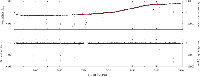
Figure 1: Upper panel. EVEREST photometry for the star K2-113 (black points) along with the 20-hour median filter smoothed with a 3-hour gaussian filter (red line), which captures the intrinsic variability of the star. Lower panel. Photometry normalized with respect to our filter.

2.2 Spectroscopic follow-up

In order to confirm the planetary nature of our candidate, high-resolution spectroscopic follow-up was performed with the FEROS spectrograph (feros:1998) mounted on the MPG 2.2m telescope located at La Silla Observatory in August (3 spectra) and November (6 spectra) of 2016, in order to obtain both initial stellar parameters for the candidate stellar host and high-precision radial velocity (RV) measurements. The spectra were obtained with the simultaneous calibration method, in which a ThAr calibration lamp is observed in a comparison fiber next to the science fiber, allowing us to trace instrumental RV drifts. The data was reduced with a dedicated pipeline (CERES; jordan:2014; ceres:2016) which, in addition to the radial-velocities and bisector spans, also calculates rough atmospheric parameters for the target star. This indicated the candidate host star was a G dwarf, with an effective temperature of $T_{\textnormal{eff}}=5500\pm 100$ K, surface log-gravity of $\log g_{*}=4.2\pm 0.3$ dex and a metallicity of $\textnormal{[Fe/H]}=0.2\pm 0.1$ dex, all very much consistent with solar values.

The obtained RVs phased up nicely with the photometric ephemerides, hinting at a semi-amplitude of $\sim 140$ m/s, consistent with an object of planetary nature (see Section 3). In addition, the measured bisector spans (BIS) showed no correlation with the RVs, which is illustrated on Figure 2; performing a monte-carlo simulation by assuming the errors on the RVs and BIS are gaussian gives a correlation coefficient of $\rho=0.15\pm 0.16$, which is consistent with zero. The obtained radial velocities and bisector spans are presented in Table 1. These results prompted us to perform a full analysis of the system, which we present in the next section.

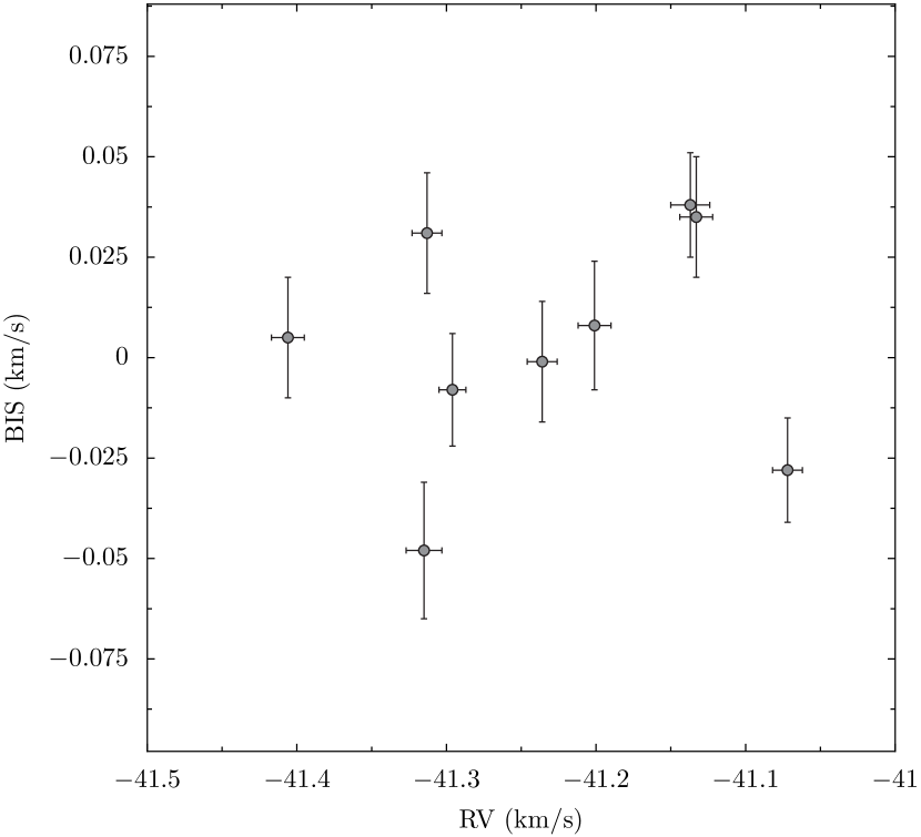
Figure 2: Radial velocity measurements versus the measured bisector spans in km/s obtained for our target star using the FEROS spectrograph. The correlation coefficient between these measurements is consistent with zero.

Table 1: Radial velocities obtained with the FEROS spectrograph along with the measured bisector spans.

Time (BJD UTC)	RV (km/s)	$\sigma_{\textnormal{RV}}$	BIS (km/s)	$\sigma_{\textnormal{BIS}}$
2457643.6804163	-41.315	0.012	-0.048	0.017
2457645.7862304	-41.236	0.010	-0.001	0.015
2457647.8755248	-41.133	0.011	0.035	0.015
2457700.7309840	-41.201	0.011	0.008	0.016
2457701.6407003	-41.313	0.010	0.031	0.015
2457702.7358066	-41.406	0.011	0.005	0.015
2457703.6386414	-41.296	0.009	-0.008	0.014
2457704.6259996	-41.137	0.013	0.038	0.013
2457705.6178241	-41.072	0.010	-0.028	0.013

3 Analysis

3.1 Stellar properties

In order to obtain the parameters of the host star, we first use the Zonal Atmospheric Stellar Parameters Estimator (ZASPE; brahm-zaspe:2016; zaspe:2016) algorithm. In brief, ZASPE compares the observed spectrum against a grid of stellar spectra in the most sensitive spectral zones to atmospheric parameters and determines the errors in the parameters by considering the systematic mismatch between the data and the models. In this case we run ZASPE on a high signal-to-noise (SNR; $\sim 100$) spectrum that was generated by co-adding the 9 individual FEROS spectra, which obtains a $T_{\textnormal{eff}}=5627\pm 88$ K, $\log g_{*}=4.400\pm 0.146$ dex, $[\textnormal{Fe/H}]=0.180\pm 0.062$ dex and projected rotational velocity $v\sin(i)=2.06\pm 0.77$ km/s, which make the host star a (slightly metal-rich) solar analogue.

In order to derive the radius, mass, age, luminosity and distance to the star, we used the latest version of the isochrones package (isochrones:2015), which uses the derived atmospheric parameters along with photometric data in order to estimate them with evolutionary tracks. The photometric data for our star was obtained from different sources; these are presented in Table 2. We used the MESA Isochrones & Stellar Tracks (MIST; dotter:2016; choi:2016) instead of the Darthmouth (dotter:2008) isochrones and stellar tracks, as the former cover wider ranges of radius, mass and age (although both gave results which were consistent within the errors). In order to explore the parameter space, the MULTINEST (multinest:2009) algorithm as implemented in PyMultinest (buchner:2014) was used because it is well suited for problems like the one at hand, which are inherenty degenerate. The derived stellar properties are presented in Table 2, all of which are consistent with the star being very similar to our own Sun ($R_{*}=1.047^{+0.11}_{-0.08}R_{\Sun}$, $M_{*}=1.007^{+0.040}_{-0.039}$, $L_{*}=1.02^{+0.24}_{-0.18}$). As can be observed, the only parameter that significatnly deviates (at 3-sigma) from that of a “solar twin" is the metallicity which, as mentioned above, is slighlty super-solar. We therefore consider the star a solar analogue.

Table 2: Stellar parameters of K2-113.

Parameter	Value	Source
Identifying Information
EPIC ID	220504338	EPIC
2MASS ID	01174783+0652080	2MASS
R.A. (J2000, h:m:s)	01${}^{h}$17${}^{m}$47.829$s$	EPIC
DEC (J2000, d:m:s)	+06${}^{o}$52${}^{\prime}$08.02${}^{\prime\prime}$	EPIC
R.A. p.m. (mas/yr)	$22.3\pm 1.7$	UCAC4
DEC p.m. (mas/yr)	$-15.8\pm 4.1$	UCAC4
Spectroscopic properties
$T_{\textnormal{eff}}$ (K)	$5627\pm 88$	ZASPE
Spectral Type	G	ZASPE
[Fe/H] (dex)	$0.180\pm 0.062$	ZASPE
$\log g_{*}$ (cgs)	$4.400\pm 0.146$	ZASPE
$v\sin(i)$ (km/s)	$2.06\pm 0.77$	ZASPE
Photometric properties
$K_{p}$ (mag)	13.51	EPIC
$B$ (mag)	$14.445\pm 0.050$	APASS
$V$ (mag)	$13.684\pm 0.030$	APASS
$g^{\prime}$ (mag)	$14.016\pm 0.030$	APASS
$r^{\prime}$ (mag)	$13.459\pm 0.020$	APASS
$i^{\prime}$ (mag)	$13.299\pm 0.030$	APASS
$J$ (mag)	$12.347\pm 0.023$	2MASS
$H$ (mag)	$11.998\pm 0.025$	2MASS
$Ks$ (mag)	$11.949\pm 0.021$	2MASS
Derived properties
$M_{*}$ ($M_{\Sun}$)	$1.007^{+0.040}_{-0.039}$	isochrones*
$R_{*}$ ($R_{\Sun}$)	$1.047^{+0.11}_{-0.08}$	isochrones*
$\rho_{*}$ (g/cm${}^{3}$)	$1.23^{+0.36}_{-0.32}$	isochrones*
$L_{*}$ ($L_{\Sun}$)	$1.02^{+0.24}_{-0.18}$	isochrones*
Distance (pc)	$553.4^{+59.0}_{-43.0}$	isochrones*
Age (Gyr)	$5.9^{+2.7}_{-3.4}$	isochrones*

Note. Logarithms given in base 10.

*: Using stellar parameters obtained from ZASPE.

3.2 Planet scenario validation

We performed a blend analysis following hartman:2011; hartman:2011a, which attempts to model the available light curves, photometry calibrated to an absolute scale, and spectroscopically determined stellar atmospheric parameters, using combinations of stars with parameters constrained to lie on the girardi:2000 evolutionary tracks. Possible blend scenarios include blended eclipsing binary (bEB) and hierchical triple (hEBs) systems. The analysis includes fits of the secondary eclipses and out of transit variations using the photometric data. We find that the data are best described by a planet transiting a star. All of the above mentioned blend scenarios are rejected at more than $5-\sigma$ using the photometry alone. Including the RV data, the scenarios are further ruled out: the simulated RVs for the blend model that provides the best fit to the photometric data imply variations in RV on the order of 500 m/s, which are much higher than what we observe. Based on this analysis, we consider our planet validated.

It is important to note that with our validation procedures, we can’t rule out the possibility that the planetary transit is being diluted by a star whithin the 12” aperture radius used to obtain the K2 photometry. However, there is no known blending source within this radius in catalogs such as the Gaia Data Release 1 (gaia:2016) and UCAC4 (zacharias:2013), while there is some stars within the 12” aperture in the Sloan Digital Sky Survey (SDSS) that have $g>20$, which would produce negligible dilutions in the K2 lightcurve.

3.3 Joint analysis

As in brahm:2016, the joint analysis of the K2 photometry and the FEROS RVs was performed using the EXOplanet traNsits and rAdIal veLocity fittER (EXONAILER; espinoza:2016) algorithm, which is available at GitHub. The algorithm makes use of the batman package (batman:2015) in order to perform the transit modelling, which has the advantage of allowing the usage of any limb-darkening law, which has been proven to be of importance if unbiased transit parameters are to be retrieved from high-precision photometry (EJ15). As recommended in the study of EJ15, we decided to let the limb-darkening coefficients be free parameters in the fit. Following the procedures outlined in EJ16, we concluded that the square-root law is the optimal law to use in our case, as this is the law that retrieves the smaller mean-squared error (i.e., the best bias/variance trade-off) on the planet-to-star radius ratio, which is the most important parameter to derive for this exoplanet, as it defines the planetary density. The mean-squared error was estimated by sampling lightcurves with similar geometric, noise and sampling properties as the observed transit lightcurve, taking the spectroscopic information in order to model the real, underlying limb-darkening effect of the star. We sampled the coefficients of this law in our joint analysis using the efficient uninformative sampling scheme outlined in kipping:2013. In order to take into account the smearing of the lightcurve due to the $\sim 27$ minute “exposures" of the Kepler long-cadence observations, we use the selective resampling technique described in resampling with $N=20$ resampled points per data-point in our analysis.

The RV analysis in our exonailer fit includes a radial-velocity jitter term that is added in quadrature to the measured uncertainties. We tried both, circular and non-circular models, but computing the BIC-based evidence of both models the non-circular model was indistinguishable from the circular one (the evidence for the non-circular model was $\sim 1.4$ that of the circular model). As such, we decided to use the most parsimonious model of both, and fixed the eccentricity to zero. We note that the non-circular model allowed us to put a 3-sigma upper limit on the eccentricity of $e<0.13$. Figure 3 shows the phase-folded photometry along with the best-fit model and Figure 4 shows the radial-velocity measurements and the corresponding best-fit model from our joint analysis. Table 3 presents the retrieved parameters. Note the moderate jitter of the star, on the order of $\sigma_{\textnormal{RV}}\sim 20$ m/s. As can be observed, the planet has a radius of $R_{p}=0.93^{+0.10}_{-0.07}R_{\textnormal{J}}$, and a mass of $M_{p}=1.29^{+0.13}_{-0.14}M_{\textnormal{J}}$, giving a density of $1.97^{+0.60}_{-0.53}$ gr/cm${}^{3}$ for this planet, wich is on the high side when compared to a “typical" hot-Jupiter (where $\rho_{p}\lesssim 1$ g/cm${}^{3}$). We discuss these planetary parameters in the context of the discovered exoplanets in the next section.

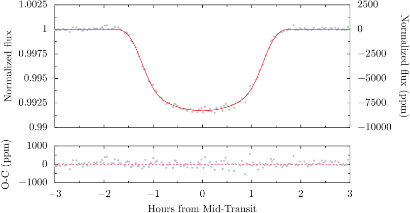
Figure 3: Phase-folded K2 photometry along with the best-fit transit model obtained from the joint analysis peformed with the EXONAILER algorithm.

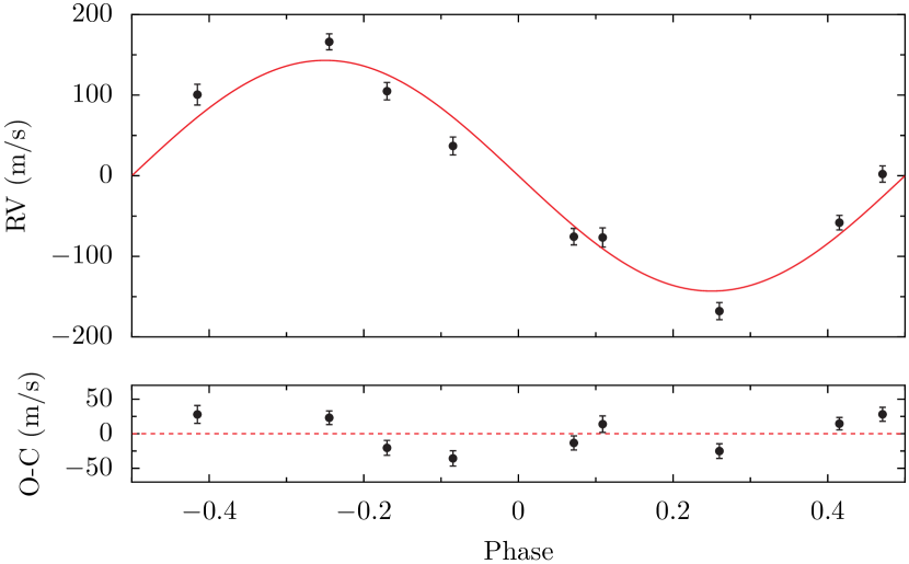
Figure 4: Phase-folded FEROS radial-velocities along with the best-fit model obtained from the joint analysis peformed with the EXONAILER algorithm.

Table 3: Orbital and planetary parameters for K2-113b.

Parameter	Prior	Posterior Value
Lightcurve parameters
$P$ (days)	$\mathcal{N}(5.8177,0.1)$	5.817608${}^{+0.000031}_{-0.000029}$
$T_{0}-2450000$ (BJD)	$\mathcal{N}(7392.88575,0.1)$	7392.88605${}^{+0.00019}_{-0.00019}$
$a/R_{\star}$	$\mathcal{U}(1,15)$	$11.39^{+0.32}_{-0.32}$
$R_{p}/R_{\star}$	$\mathcal{U}(0.01,0.2)$	$0.0911^{+0.00070}_{-0.00083}$
$i$ (deg)	$\mathcal{U}(70,90)$	86.21${}^{+0.20}_{-0.21}$
$q_{1}$ ${}^{a}$	$\mathcal{U}(0,1)$	$0.72^{+0.17}_{-0.16}$
$q_{2}$ ${}^{a}$	$\mathcal{U}(0,1)$	$0.33^{+0.11}_{-0.15}$
$\sigma_{w}$ (ppm)	$\mathcal{J}(10,500)$	138.4${}^{+1.8}_{-1.6}$
RV parameters
$K$ (m s${}^{-1}$)	$\mathcal{N}(0,100)$	$144.5^{+13.5}_{-15.4}$
$\mu$ (km s${}^{-1}$)	$\mathcal{N}(-41.24,0.01)$	$-41.2375^{+0.0063}_{-0.0065}$
$\sigma_{\textnormal{RV}}$ (m s${}^{-1}$)	$\mathcal{J}(1,100)$	$24.3^{+10.1}_{-6.6}$
$e$	—	$0$ (fixed; upper limit${}^{c}$ $e<0.13$)
Derived Parameters
$s_{1}$ ${}^{a}$		$0.30^{+0.20}_{-0.19}$
$s_{2}$ ${}^{a}$		$0.55^{+0.26}_{-0.29}$
$M_{p}$ ($M_{\textnormal{J}}$)	—	$1.29^{+0.13}_{-0.14}$
$R_{p}$ ($R_{\textnormal{J}}$)	—	$0.93^{+0.10}_{-0.07}$
$\rho_{p}$ (g/cm${}^{3}$)	—	$1.97^{+0.61}_{-0.53}$
$\log g_{p}$ (cgs)	—	$3.56^{+0.08}_{-0.10}$
$a$ (AU)	—	$0.0558^{+0.0059}_{-0.0049}$
$\log\langle F\rangle$ (cgs)${}^{b}$	—	$8.640^{+0.033}_{-0.034}$
$V_{\textnormal{esc}}$ (km/s)	—	$69.7^{+4.9}_{-4.8}$
$T^{d}_{\textnormal{eq}}$ (K)
Bond albedo of $0.0$	—	$1178^{+22}_{-23}$
Bond albedo of $0.75$	—	$833^{+16}_{-16}$

Note. Logarithms given in base 10. $\mathcal{N}(\mu,\sigma)$ stands for a normal prior with mean $\mu$ and standard-deviation $\sigma$, $\mathcal{U}(a,b)$ stands for a uniform prior with limits $a$ and $b$ and $\mathcal{J}(a,b)$ stands for a Jeffrey’s prior with the same limits. Times are given in BJD TDB.
${}^{a}$The $q_{1}$ and $q_{2}$ parameters are the triangular sampling coefficients used to fit for the square-root limb-darkening law (kipping:2013). The $s_{1}$ and $s_{2}$ limb-darkening coefficients are recovered by the transformation $s_{1}=\sqrt{q_{1}}(1-2q_{1})$ and $s_{2}=2\sqrt{q_{1}}q_{2}$.
${}^{b}$Orbit averaged incident stellar flux on the planet.
${}^{c}$3-sigma upper limit obtained from a non-circular joint fit to the data (see text).
${}^{d}$Full energy redistribution has been assumed.