Optimal Pricing for Submodular Valuations with Bounded Curvature

Abstract

The optimal pricing problem is a fundamental problem that arises in combinatorial auctions. Suppose that there is one seller who has indivisible items and multiple buyers who want to purchase a combination of the items. The seller wants to sell his items for the highest possible prices, and each buyer wants to maximize his utility (i.e., valuation minus payment) as long as his payment does not exceed his budget. The optimal pricing problem seeks a price of each item and an assignment of items to buyers such that every buyer achieves the maximum utility under the prices. The goal of the problem is to maximize the total payment from buyers. In this paper, we consider the case that the valuations are submodular. We show that the problem is computationally hard even if there exists only one buyer. Then we propose approximation algorithms for the unlimited budget case. We also extend the algorithm for the limited budget case when there exists one buyer and multiple buyers collaborate with each other.

1 Introduction

1.1 Background and motivation

In a combinatorial auction (?; ?), a seller has a set of indivisible items, and buyers purchase a combination of the items. The seller wants to sell his items to the buyers for the highest possible prices, and each buyer wants to purchase a set of items that is valuable for him and also has a reasonable price. More precisely, each buyer purchases a set of items that maximizes his utility within the limits of his budget; here, the utility for a set of items is the valuation for him (minus the payment for purchase). Thus, the seller seeks a price of each item (not bundle) and an assignment of items to buyers such that they are stable, i.e., no buyer can gain more utility by changing the set of items that he purchases. The goal is to maximize the total profit obtained from the buyers. The stability captures a fairness condition for the individual buyers (?; ?; ?; ?). In general, such a problem is called the optimal pricing problem and studied in many situations.

In this paper, we assume that the valuations of buyers are represented by submodular functions, which capture the notion of the diminishing returns property. Submodular functions appear in many situations (?; ?), and have been studied extensively. For simplicity, we assume that every buyer truthfully tells the seller his valuation and his budget. The purpose of this paper is to analyze theoretical properties of the optimal pricing problems with submodular valuations, and to propose (approximation) algorithms for the problems. We analyze the performance of the algorithms in terms of the curvatures of the valuations, which capture the degree of nonlinearity. The curvature has been used to derive better approximation ratios for several submodular optimization problems (?; ?; ?; ?).

1.2 Our contributions

We summarize our results for the optimal pricing problem.

We first show that the optimal pricing problem with submodular valuations is NP-hard even for instances derived from our application (Theorem 5). Moreover, there exists an instance that requires exponentially many oracle evaluations in the oracle model (Theorem 6).

Our main result is to propose approximate pricing algorithms for the following three cases: single buyer case (Algorithm 1), multiple buyers case (Algorithm 2), and multiple collaborating buyers case (Algorithm 3). Then we show the approximation ratios for these algorithms in terms of the curvatures of the valuations (Theorems 7, 10, 12). Our algorithms output a nearly optimal solution if the curvatures are small. We will point out that a practical application of our problem has submodular valuations whose curvatures are typically small by using a general upper bound on curvatures (Theorem 2). This justifies our analysis of the optimal pricing problem using curvatures. The application is a similar problem to the budget allocation problem, which is widely studied both theoretically and practically in computational advertising. We include all the proofs in the Appendix.

We also conduct computational experiments on some synthetic and realistic datasets to evaluate the proposed pricing algorithms (Section 6). Our algorithm performs better than baseline algorithms. To the best of our knowledge, no prior work proposed a suitable algorithm for the optimal pricing problem with submodular valuations.

1.3 Related Work

The optimal pricing problem is also referred to as the profit maximizing pricing problem. There are many works for the case when valuations of buyers are unit-demand or single-minded  (?; ?; ?; ?; ?; ?). A valuation $f$ is called unit-demand if $f(X)=\max_{x\in X}f(x)$ for any $X$ with $|X|\geq 2$, and called single-minded if for some $S^{*}$, it holds that $f(X)=f(S^{*})>0$ for any $X\supseteq S^{*}$ and $f(X)=0$ otherwise. Any unit-demand valuation is submodular, while single-minded valuations are not necessarily submodular. Guruswami et al. (?) proved the APX-hardness of the optimal pricing problem where the valuations are all unit-demand or all single-minded. Thus, the general optimal pricing problem is computationally intractable. They also provided logarithmic approximation algorithms under the assumption that the valuations are all unit-demand or all single-minded. Since these algorithms fully rely on the assumption, they do not extend to our case.

We remark that the optimal pricing problem is different from the problem of finding a Walrasian equilibrium. A pair of a pricing and an assignment is called a Walrasian equilibrium (or competitive equilibrium) if it is stable and all positive-price items are allocated to some buyer (?). In our model, the seller can decide a subset of items that are not allocated. This difference may improve the seller’s profit. We give such an example in Remark 8.

The winner determination problem is also similar to the optimal pricing problem. This is the problem of finding an allocation of items to buyers that maximizes the sum of buyers’ valuations in combinatorial auctions. Rothkopf et al. (?) proved the NP-hardness of the winner determination problem. Sandholm (?) provided an inapproximability result on the problem and some approximation algorithms for special cases. For more details of this problem, see, e.g., (?; ?). The winner determination problem maximizes the total valuation of buyers whereas our problem maximizes the profit of the seller. In general, these problems have different optimal solutions (see Remark 8 for an example). So our problem setting is different from the winner determination problem.

2 Preliminaries

In this section, we review submodular functions and the optimal pricing problem, and describe our motivation to study the optimal pricing problem.

2.1 Submodular function and curvature

Let $V$ be a finite set. A function $f:2^{V}\to\mathbb{R}$ is submodular if it satisfies

$$f(X)+f(Y)\geq f(X\cap Y)+f(X\cup Y)$$ (1)

for all $X,Y\subseteq V$ (?). This condition is equivalent to the diminishing returns property: $f(X)-f(X\setminus x)\geq f(Y)-f(Y\setminus x)$ for all $X\subseteq Y\subseteq V$; here we denote “$X\setminus\{x\}$” by “$X\setminus x$” for notational simplicity. We say that $f$ is monotone nondecreasing if $f(X)\leq f(Y)$ for all $X\subseteq Y$. In this paper, we assume that $f(\emptyset)=0$.

The diminishing returns property is a fundamental principle of economics (?). Thus, submodular functions are often used to model user utilities and preferences. They also appear in combinatorial optimization (?; ?), social network analysis (?), and machine learning (?; ?; ?).

For a monotone nondecreasing function $f:2^{V}\to\mathbb{R}$ and an integer $s\in\{0,\ldots,|V|\}$, the curvature $\kappa(s)$ is defined by the largest nonnegative number that satisfies

$$(1-\kappa(s))f(x)\leq f(X)-f(X\setminus x)$$ (2)

for all $|X|=s$ and $x\in X$ (?). If $f$ is submodular, then its curvature $\kappa(s)$ is a monotone nondecreasing sequence by the diminishing returns property.

We remark that computing $\kappa(s)$ is difficult since it requires exponentially many function evaluations; therefore, we cannot use explicitly the value in an algorithm.

2.2 Optimal pricing problem

Here we define the optimal pricing problem. Suppose that a seller wants to sell indivisible items $V$ to buyers $N=\{1,\ldots,n\}$ simultaneously. Each buyer $i\in N$ has a budget $B_{i}$ and a valuation function $f_{i}:2^{V}\to\mathbb{R}$, where $f_{i}$ is a monotone nondecreasing submodular function. We denote by $\kappa_{i}$ the curvature of $f_{i}$ for $i\in N$. In this problem, we find a price vector $p\in\mathbb{R}^{V}$ and an assignment $(X_{1},\ldots,X_{n})$ which is a subdivision of $V$. For a price vector $p$ and an item set $X\subseteq V$, let $p(X)=\sum_{x\in X}p(x)$. Buyers are assumed to have quasi-linear utility, i.e., the utility of $i\in N$ is given by $f_{i}(X_{i})-p(X_{i})$.

The seller wants to maximize the total profit $p(X_{1})+\cdots+p(X_{n})$. On the other hand, each buyer also wants to maximize his utility, as long as his payment to the seller does not exceed his budget. Therefore, the assignment must satisfy some “agreement” condition. We say that a price vector $p$ and assignment $(X_{1},\ldots,X_{n})$ pair is stable if it satisfies

$$f_{i}(X_{i})-p(X_{i})\geq f_{i}(X)-p(X)$$ (3)

for any $i\in N$ and all $X\subseteq V$. The stability condition means that each buyer $i$ has no incentive to change his allocation $X_{i}$ under the pricing $p$. For a price vector $p$, we define the demand set of buyer $i$ as a family of sets $X$ satisfying (3), denoted by

$$D_{i}(p)=\operatornamewithlimits{argmax}\{f_{i}(X)-p(X)\mid X\subseteq V,\ p(X)\leq B_{i}\}.$$ (4)

The stability condition is necessary to avoid a grudge or an antipathy of buyers even when each buyer $i$ knows his own allocated items $X_{i}$ and every price of the items $V$.

The optimal pricing problem seeks a price vector $p\in\mathbb{R}^{V}$ and an assignment $(X_{1},\ldots,X_{n})$ that maximizes the total profit $p(X_{1})+\cdots+p(X_{n})$ under the stability condition. It is formulated as

maximize $$\textstyle\quad\sum_{i\in N}p(X_{i})$$

subject to $$\quad X_{i}\in D_{i}(p)~{}(i\in N),$$ (5)

$$\quad X_{i}\cap X_{j}=\emptyset~{}(i\neq j).$$

We propose algorithms for the problem (5) where all buyers have unlimited budgets, i.e., $B_{i}=+\infty$ for all $i\in N$. We extend our results to the limited budget case (see (?)).

2.3 Application

We present an application that motivates us to study the optimal pricing problem with submodular valuations. We will claim that the curvatures of valuations are small in practice.

Consider that the publisher (= seller) has a set $V$ of marketing channels, and that there is a set $N$ of advertisers (= buyers) that have budgets $B_{i}\ (i\in N)$ . Each advertiser $i\in N$ purchases a subset $X$ of channels for advertising under the budget constraint, i.e., $p(X)\leq B_{i}$. The valuation $f_{i}(X)$ of $X\subseteq V$ for advertiser $i$ is the expected value of the total revenue from loyal customers influenced by marketing channels in $X$. Let $p\in\mathbb{R}^{V}$ be the price vector, i.e., $p(v)$ is the price to publish an advertisement through marketing channel $v$. Each advertiser $i$ wants to buy $X_{i}$ that maximizes the total revenue minus the cost, i.e., $f_{i}(X_{i})-p(X_{i})$, under the budget constraint $p(X_{i})\leq B_{i}$. In the following, we explicitly formulate the valuation function $f_{i}$ of each advertiser $i$.

We adopt the bipartite influence model of advertising proposed by Alon et al. (?). Let $W$ be set of customers. We consider a bipartite graph $G=(V\cup W,E)$. Each edge $(v,w)\in E$ indicates that marketing channel $v$ affects customer $w$. Each edge $(v,w)$ is assigned probabilities $q_{i}(v,w)\ (i\in N)$, called activation probability. If advertiser $i$ puts an advertisement on marketing channel $v$, then customer $w$ will become a loyal customer of buyer $i$ with probability $q_{i}(v,w)$.

The probability $Q_{i}(X,w)$ that customer $w$ becomes a loyal customer when a advertiser $i$ runs advertisements on $X\subseteq V$ is given by $Q_{i}(X,w)=1-\prod_{x\in X,(x,w)\in E}(1-q_{i}(x,w))$. Thus, the expected number of his loyal customers is $\sum_{w\in W}Q_{i}(X,w)$. Let $\gamma_{i}$ be the expected revenue from one loyal customer. The expected total revenue is given by

$$\textstyle f_{i}(X)=\gamma_{i}\cdot\sum_{w\in W}Q_{i}(X,w).$$ (6)

Since $Q_{i}(X,w)$ is a monotone nondecreasing submodular function in $X$, $f_{i}(X)$ is also a monotone nondecreasing submodular function.

Here, we can observe that each curvature $\kappa_{i}$ of $f_{i}$ is small ($i\in N$). This implies that our analysis based on the curvature is particularly effective for this application.

Lemma 1.

For each $i\in N$ and $s\in\{1,\ldots,|V|\}$, $\kappa_{i}(s)\leq\max_{|X|=s,~{}x\in X,~{}(x,w)\in E}Q(X\setminus x,w)$.

Theorem 2.

For each $i\in N$ and $s\in\{1,\ldots,|V|\}$, if $q_{i}(e)\leq q$ for any $e\in E$, then it holds that $\kappa_{i}(s)\leq 1-(1-q)^{\min\{s,d\}-1}$, where $d$ is the maximum degree of the right vertices $W$.

In practice, $d$ is relatively small (e.g., $d\leq 100$) since it is the number of incoming information channels of a customer. Moreover, $q$ is very small (e.g., $q\leq 0.001$) since it is the probability of gaining a customer through a single advertisement.

3 Single buyer

In this section, we analyze the optimal pricing problem with a single buyer (i.e., $n=1$). We prove the NP-hardness of the problem and present a nearly optimal approximate algorithm for the buyer with an unlimited budget.

Consider that there is only one buyer with an unlimited budget. For notational convenience, let $f:2^{V}\to\mathbb{R}$ be his valuation, which is a monotone nondecreasing submodular function. For a price vector $p$, we denote by $D(p)$ the demand set for $p$. When we fix an assignment, we can easily obtain the maximum profit for the assignment.

Lemma 3.

Let $X$ be an assignment. An optimal price vector for (5) with fixed $X$ is given by $p(x)=f(X)-f(X\setminus x)$ if $x\in X$, and $p(x)=+\infty$ otherwise.

From this lemma, we obtain the following characterization of optimal solutions to (5).

Lemma 4.

Let $X$ be an assignment. There exists a price vector $p$ such that $(p,X)$ is optimal to (5) if and only if $X$ achieves

$$\textstyle\max_{X^{\prime}\subseteq V}\sum_{x\in X^{\prime}}(f(X^{\prime})-f(X^{\prime}\setminus x)).$$ (7)

This implies that problem (5) is equivalent to (7). For any $X\subseteq V$, we denote $h(X)=\sum_{x\in X}(f(X)-f(X\setminus x))$.

We show the NP-hardness of (5) by reducing the one-in-three positive 3-SAT problem. Given a boolean formula in conjunctive normal form with three positive literals per clause, the one-in-three positive 3-SAT problem determines whether there exists a truth assignment to the variables so that each clause has exactly one true variable. This problem is known to be NP-complete (?).

Theorem 5.

Problem (5) is NP-hard even when the function $f$ is of the form (6).

Furthermore, we obtain the result below.

Theorem 6.

If $f$ is given by an oracle, problem (5) requires exponentially many oracle evaluations.

Since (5) is NP-hard, we propose an algorithm to find an approximate pricing. Once we determine an assignment, an optimal price vector for the assignment is easily obtained from Lemma 3. Thus, we only need to find an assignment $X$ maximizing $h(X)$. However, an overly large assignment $X$ may have small $h(X)$ value. In our algorithm, we assign the top $s$ elements in order of their value, for each $s=1,\ldots,|V|$. The formal description is given in Algorithm 1.

Algorithm 1 Pricing algorithm for a single buyer.

  For $s=1,2,\ldots,|V|$

   Let $X^{s}$ be the largest $s$ elements of $f(x)$

   Price $p^{s}(x)=f(X^{s})-f(X^{s}\setminus x)$ $(x\in X^{s})$ and $p^{s}(y)=+\infty$ $(y\in V\setminus X^{s})$

  Return $p$ and $X$ that attains maximum of $p^{s}(X^{s})$

This algorithm can be implemented to run in $O(|V|\log|V|+A|V|^{2})$ time, where $A$ is the computational cost of evaluating $f(X)$. For a variant of budget allocation problem with the bipartite graph model, if we implement the algorithm carefully, it runs in $O(|V||E|)$ time.

We analyze the approximation ratio of our algorithm.

Theorem 7.

Let $(p^{*},X^{*})$ be an optimal solution to (5), and let $(p,X)$ be the output of Algorithm 1. Then, it holds that $X\in D(p)$ and $(1-\kappa(|X^{*}|))p^{*}(X^{*})\leq p(X)$.

Remark 8.

Selling all items (i.e., $s=|V|$) is not always optimal, even when the function $f$ is of the form (6). To demonstrate this, let us consider the instance of the application in Section (2.3) where there are two channels $u,v$ and one user $w$ with $\gamma=1$. The activation probabilities from $u$ and $v$ to $w$ are $0.9$. When we use the both channels, the activation probability is $1-(1-0.9)^{2}=0.99$. Thus $f(u)=f(v)=0.9$ and $f(u,v)=0.99$. The optimal pricing sells only a single channel $X^{*}=\{u\}$ at price $p^{*}(u)=0.9$, and $p^{*}(X^{*})=0.9$. On the other hand, to sell all items $X^{\prime}=\{u,v\}$, the price should be $p^{\prime}(u)=p^{\prime}(v)=0.99-0.9=0.09$, and hence $p^{\prime}(X^{\prime})=0.18$.

We also remark that this example shows the difference between our problem and related problems, namely, the problem of finding Walrasian equilibrium and the winner determination problem. There are two Walrasian equilibria $(p^{\prime},X^{\prime})$ and $(p^{\prime\prime},X^{\prime})$ where $p^{\prime\prime}(u)=p^{\prime\prime}(v)=0$. Thus $(p^{\prime},X^{\prime})$ achieves the maximum profit $p^{\prime}(X^{\prime})=0.18$ among Walrasian eqiulibria whereas the optimal value for our problem is $0.9$. When we regard this example as an instance of the winner determination problem, the optimal solution is $X^{\prime}$ and its valuation of the buyer is $0.99$. However, the optimal solution for our problem sells only $X^{*}$, and the profit of the seller is $0.9$.

We also show that if the curvature of $f$ is small, then the optimal values of (5) and the one without the stability condition is almost the same; see Theorem 18 and 19 in Appendix.

4 Multiple buyers

In this section, we deal with the general optimal pricing problem (5) that admits more than one buyer. Recall that if $n=1$, then for any assignment $X$, there always exists a price vector $p$ satisfying $X\in D(p)$ (see Lemma 3). However, in general, there may not exist a price vector $p$ such that $X_{i}\in D_{i}(p)$ for some assignment $(X_{1},\dots,X_{n})$. Moreover, it is difficult to determine whether or not such a price vector exists for a given assignment.

We first approach the coNP-hardness of deciding the existence of a stable price vector for a given assignment by reducing the exact cover by 3-sets problem (X3C), which is NP-complete (?). In this problem, we are given a set $E$ with $|E|=3l$ and a collection $\mathcal{C}=\{C_{1},\dots,C_{m}\}$ of 3-element subsets of $E$. The task is to decide whether or not $\mathcal{C}$ contains an exact cover for $E$, i.e., a subcollection $\mathcal{C}^{\prime}\subseteq\mathcal{C}$ such that every element of $E$ occurs in exactly one member of $\mathcal{C}^{\prime}$.

Theorem 9.

It is coNP-hard to determine, for a given assignment $(X_{1},\dots,X_{n})$, the existence of price vector $p$ such that $X_{i}\in D_{i}(p)$ for all $i\in N$.

We also show that, given a price vector $p$, it is NP-hard to decide the existence of an assignment $\mathbf{X}=(X_{1},\dots,X_{n})$ such that $(p,\mathbf{X})$ is stable (Theorem 20 in Appendix).

By above results, it is difficult to find a stable pair $(p,\mathbf{X})$ for given $p$ (or $\mathbf{X}$). Therefore in order to obtain efficiently an approximate solution, we take a natural approach that we slightly relax the stability condition.

For any positive number $\alpha\leq 1$ and each buyer $i$, we define the $\alpha$-demand set of buyer $i$ as $D^{\alpha}_{i}(p)=\left\{X\subseteq V\mid f_{i}(X)-p(X)\geq\alpha f_{i}(Y)-p(Y),\ \forall Y\subseteq V\right\}$. For a price vector $p$ and an assignment $\mathbf{X}=(X_{1},\dots,X_{n})$, we say that $(p,\mathbf{X})$ is $\alpha$-stable if $X_{i}\in D^{\alpha}_{i}$ for all $i\in N$.

Algorithm 2 Pricing algorithm for multiple buyers

  For $s=1,2,\ldots,|V|$

   Let $X^{s}$ be $s$ largest elements of $\max_{i\in N}f_{i}(x)$

   Price $p^{s}(x)=\max_{i\in N}(f_{i}(X^{s})-f_{i}(X^{s}\setminus x))$ $(x\in X^{s})$ and $p^{s}(y)=+\infty$ $(y\in V\setminus X^{s})$

   Let $(X^{s}_{1},\dots,X^{s}_{n})$ be a partition of $X^{s}$ such that $p^{s}(x)=f_{i}(X^{s})-f_{i}(X^{s}\setminus x)~{}(\forall x\in X^{s})$

  Return $p$ and $(X_{1},\dots,X_{n})$ that attains maximum of $\sum_{i\in N}p^{s}(X^{s}_{i})$

We propose a pricing algorithm in Algorithm 2. The algorithm can be implemented to run in $O(An|V|^{2}+|V|\log|V|)$ time, where $A$ is the computational cost of evaluating $f_{i}(X)$ ($i\in N$). It has the following theoretical guarantee. Here we denote $\kappa(s)=\max\kappa_{i}(s)$.

Theorem 10.

Let $p^{*}$ and $\mathbf{X}^{*}=(X_{1}^{*},\ldots,X_{n}^{*})$ be the optimal solution to (5) and let $p$ and $\mathbf{X}=(X_{1},\ldots,X_{n})$ be the solution obtained by Algorithm 2. Then, for $s=|X_{1}\cup\cdots\cup X_{n}|$ and $s^{*}=|X_{1}^{*}\cup\cdots\cup X_{n}^{*}|$, $(p,\mathbf{X})$ is $(1-\kappa(s))$-stable and $(1-\kappa(s^{*}))\sum_{i\in N}p^{*}(X_{i}^{*})\leq\sum_{i\in N}p(X_{i})$.

5 Multiple collaborating buyers

In this section, we analyze the optimal pricing problem with collaborating buyers, i.e., the case where buyers cooperate to maximize the total utilities. This occurs when buyers are employed by the same organization. We present an approximation algorithm for this problem.

We first describe the model. Assume that there are buyers $N=\{1,\ldots,n\}$, whose valuation functions are given by $f_{1},\ldots,f_{n}$. Let $(X_{1},\ldots,X_{n})$ be an assignment. Since the goal of buyers is to maximize the sum of their utilities, the stability condition is written as $\sum_{i\in N}(f_{i}(X_{i})-p(X_{i}))\geq\sum_{i\in N}(f_{i}(Y_{i})-p(Y_{i}))$ for any assignment $(Y_{1},\ldots,Y_{n})$.

Because only the total amount of the utilities matters, the publisher only needs to find a set $X$ and a price vector $p$ that satisfies the above stability condition for some partition of $X$. Thus, in the following, we assume that there exists one buyer who represents the set of original buyers. Let $f:2^{V}\to\mathbb{R}$ be an aggregated valuation function defined by $f(X)=\max_{(X_{1},\dots,X_{n}):\text{ partition of }X}\sum_{i\in N}f_{i}(X_{i})$ for $X\subseteq V$. Note that $f(X)$ is monotone nondecreasing but not necessarily submodular (See Example 21 in Appendix).

By using the aggregated valuation function, the stability condition is equivalent to the condition that $f(X)-p(X)\geq f(Y)-p(Y)$ for all $Y\subseteq V$. Thus, the demand set is defined as (4), and the optimal pricing problem for collaborating buyers is formulated as

$$\text{maximize}\;\;p(X)\quad\text{subject to}\;\;X\in D(p).$$ (8)

Although the aggregated valuation function is not necessarily submodular, problem (8) has a similar formulation to (5) with a single buyer. We obtain a similar result to Lemma 3.

Lemma 11.

Let $X$ be an assignment. An optimal price vector for (8) with fixed $X$ is given by $p(x)=\min_{Y\subseteq X:x\in Y}(f(Y\cup x)-f(Y))$ if $x\in X$, and $p(x)=+\infty$ otherwise.

From this lemma, we see that problem (8) is equivalent to the problem of finding $X\subseteq V$ maximizing $\sum_{x\in X}\min_{Y\subseteq X:x\in Y}(f(Y)-f(Y\setminus x))$. Thus, we can apply the same principles as the ones of Algorithm 1. In fact, setting prices $p^{s}(x)=\min_{Y\subseteq X^{s}:x\in Y}(f(Y)-f(Y\setminus x))$ implies a similar result. However, computing $f(X)$ is intractable (this problem is called submodular welfare problem) and hence it is hard to evaluate the value $\min_{Y\subseteq X:x\in Y}(f(Y)-f(Y\setminus x))$. Thus, we need a further modification.

Our algorithm, summarized in Algorithm 3, finds an approximate solution to (8) in $O(An|V|^{2}+|V|\log|V|)$ time, where $A$ is the computational cost of evaluating $f_{i}(X)$ ($i\in N$). We analyze the approximation ratio of our algorithm. Let $\kappa_{1},\ldots,\kappa_{n}$ be curvatures of $f_{1},\ldots,f_{n}$ and $\kappa(s)=\max_{j}\kappa_{j}(s)$ for $s=1,\dots,|V|$.

Algorithm 3 Pricing algorithm for collaborating buyers

  For $s=1,2,\ldots,|V|$

   Let $X^{s}$ be $s$ largest elements of $f(x)~{}(=\max_{i}f_{i}(x))$

   Price $p^{s}(x)=\min_{i\in N}\frac{f_{i}(X^{s})-f_{i}(X^{s}\setminus x)}{f_{i}(x)}f(x)$ $(x\in X^{s})$ and $p(y)=+\infty$ $(y\in V\setminus X^{s})$

  Return $p$ and $X$ that attains maximum of $p^{s}(X^{s})$

Theorem 12.

Let $(p^{*},X^{*})$ be an optimal solution to (8), and let $(p,X)$ be the output of Algorithm 3. It then holds that $X\in D(p)$ and $(1-\kappa(|X^{*}|))p^{*}(X^{*})\leq p(X)$.

To prove this theorem, we show the following two lemmas.

Lemma 13.

For a set $X$ and $x\in X$, it holds that $f(X)-f(X\setminus x)\leq f(x)$.

Lemma 14.

For a set $X$ and $x\in X$, it holds that $f(X)-f(X\setminus x)\geq\min_{i\in N}\frac{f_{i}(X)-f_{i}(X\setminus x)}{f_{i}(x)}f(x)\geq(1-\kappa(|X|))f(x)$.

6 Experiments

In this section, we present experimental results on our pricing algorithms for a variant of budget allocation problem, which are described in Section 2.3. All experiments were conducted on an Intel Xeon E5-2690 2.90GHz CPU (32 cores) with 256GB memory running Ubuntu 12.04. All codes were implemented in Python 2.7.3.

We performed the following five experiments: For the single advertiser case, (1) we computed prices of each channel for a realistic dataset; (2) we compared the proposed algorithm with other baseline algorithms; (3) we evaluated the scalability of the proposed algorithm; and (4) we observed the relationship between the activation probabilities and the number of allocated channels. For the multiple advertisers case and the multiple collaborating advertisers case, (5) we observed the relationship between the obtained profit and the number of advertisers.

For these experiments, we used two random synthetic networks (Uniform, PowerLaw) and three networks constructed from real-world datasets (Last.fm, MovieLens, BookCrossing). Throughout the experiments, we assume that the expected revenue from one loyal customer is $1$, i.e., $\gamma_{i}=1$. The description of the datasets is given in Appendix.

(1) Typical result

First, we ran Algorithm 1 to Last.fm dataset to compute prices for the musics played in Last.fm. Top 10 frequently played musics and top 10 high price musics are displayed in Table 1 and Table 2, respectively. We can observe that some musics with a large number of plays (or unique users) are not assigned high prices. This occurs because of the stability condition.

Table 1: Ranking by #plays.

rank	artist – music	#play	UU
1	The Postal Service – Such Great Heights	3992	321
2	Boy Division – Love Will Tear Us Apart	3663	318
3	Radiohead – Karma Police	3534	346
4	Muse – Supermassive Black Hole	3483	263
5	Death Cab For Cutie – Soul Meets Body	3479	233
6	The Knife – Heartbeats	3156	177
7	Muse – Starlight	3060	260
8	Arcade Fire – Rebellion (Lies)	3048	292
9	Britney Spears – Gimme More	3004	59
10	The Killers – When You Were Young	2998	235

Table 2: Ranking by prices.

rank	original	artist – music	price
1	1	The Postal Service – Such Great Heights	3.330
2	8	Arcade Fire – Rebellion (Lies)	2.101
3	4	Muse – Supermassive Black Hole	2.029
4	11	Interpol – Evil	2.026
5	3	Radiohead – Karma Police	2.003
6	6	The Knife – Heartbeats	1.992
7	12	Kanye West – Love Lockdown	1.893
8	17	Arcade Fire – Neighborhood #1 (Tunnels)	1.868
9	23	Kanye West – Heartless	1.788
10	24	Radiohead – Nude	1.770

(2) Comparison with other pricing algorithms

Table 3: Comparison of pricing algorithms on several datasets. Each value is the ratio of the profit obtained by the algorithm and the proposed algorithm.

	Proposed	SellAll	Random	Scaled	Ascend
Uniform	1.00	0.89	0.55	0.98	0.96
PowerLaw	1.00	0.89	0.65	0.98	0.51
Last.fm	1.00	0.71	0.46	0.99	0.78
MovieLens	1.00	0.58	0.48	0.96	0.67
BookCrossing	1.00	1.00	0.39	0.78	0.43

Next, we compared Algorithm 1 with the following four baseline algorithms:

Selling all items.

Assign $X=V$ and price $p(v)=f(V)-f(V\setminus v)$ for each $v\in V$. This algorithm gives a stable assignment.

Random pricing.

Price $p(v)\in[0,f(v)]$ uniformly at random for each $v\in V$ and find an assignment $X$ by the greedy algorithm.

Scaled pricing.

Price $p(v)=\alpha f(v)$ for each $v$ and find an assignment $X$ by the greedy algorithm. $\alpha$ is chosen optimally from $\{0.1,\ldots,1.0\}$.

Ascending pricing.

Start from $X=V$ and $p(v)=0\ (v\in V)$, repeat the following process: Price $p(v)=\min_{X:x\in X}(f(X)-f(X\setminus x))$ for each $v\in X$, remove $\tilde{x}$ that attains the minimum from $X$, and then price $p(\tilde{x})=+\infty$. This algorithm is motivated by the ascending auction (?).

We remark that there are no existing algorithms that are directly applicable to the optimal pricing problem with submodular valuations (see also Section 1.3).

We used all the networks described above; we set $|V|=100$, $|W|=10000$, $d=10$ and $q_{\text{max}}=0.3$ for Uniform and PowerLaw. The result is summarized in Table 3. The proposed algorithm outperforms all compared algorithms for all datasets

(3) Scalability

We evaluated the scalability of the proposed algorithm. We used Uniform with $|V|\in\{16,32,\ldots,1024\}$, $|W|\in\{100,1000,10000,100000\}$, $d=10$, and $q_{\text{max}}=0.3$. We also conducted the same experiment on PowerLaw but we omit it since it yields very similar results.

The result is shown in Figure 2. The elapsed times were (roughly) proportional to both $|V|$ and $|W|$. This is consistent with our analysis that the proposed algorithm runs in $O(|V||E|)$ time, and the number of edges is proportional to $|W|$ for these networks. Therefore, the proposed algorithm scales to moderately large networks.

(4) Number of allocated channels and activation probabilities

We observe the relationship between activation probability and the obtained allocation. We used Uniform and PowerLaw with the parameters $|V|=100$, $|W|=10000$, and $d=10$. We controlled the maximum activation probability $q_{\text{max}}\in\{0.05,0.10,\ldots,0.95\}$ and observe the number of assigned marketing channels.

The result is shown in Figure 2. For both networks, when $q_{\text{max}}$ was small the proposed algorithm assigned all channels, and when $q_{\text{max}}$ was large it assigned a few channels. The number of assigned channels decreased much faster in PowerLaw than in Uniform, since there were highly correlated marketing channels in PowerLaw.

(5) Profit and the number of advertisers

Next, we conducted experiments on the multiple advertisers case and the multiple collaborating advertisers case. Here we observe the relationship between the profit and the number of advertisers in these settings. For these experiments, we modified Uniform and PowerLaw to assign multiple probabilities $q_{1}(e),\ldots,q_{n}(e)$ for each edge, each of which follows the uniform distribution on $[0,q_{\text{max}}]$.

The result is shown in Figure 3. By comparing two results obtained by the multiple (non-collaborating) advertisers case, the number of advertisers had little influence on the profit. On the other hand, by comparing the results obtained by collaborating advertisers, the profit increased when the number of advertisers increased. Moreover, the profits obtained from the collaborating advertisers consistently outperformed those obtained from non-collaborating advertisers. This means that collaboration of advertisers yields a better profit to the publisher. Note that we could not observe the difference between Uniform and PowerLaw.

Figure 1: Scalability of the proposed algorithm.   Figure 2: The number of assigned channels versus edge probability.

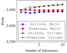
Figure 3: Profit versus the number of non-collaborating or collaborating advertisers.

7 Conclusion

We propose some future works. One is to develop an approximate pricing algorithm for the case that multiple buyers have limited budgets. Another one is to analyze the optimal pricing problem with multiple sellers. In this study, we assumed there is one seller; who can be regarded as a monopolist. The seller can select both the assignment and the price as long as they satisfy the stability condition. This situation is highly advantageous for the seller. Finally, in this study, we do not consider nonlinear or non-anonymous pricing. It would be interesting in future work to analyze the effect of such generalizations of pricing.

Acknowledgments This work was supported by JSPS KAKENHI Grant Number 16K16011, and JST, ERATO, Kawarabayashi Large Graph Project.

Appendix A Extension to limited budget cases

In this section, we extend our algorithms for the optimal pricing problem with unlimited budget cases to ones for the limited budget cases.

First, suppose that there exists only one buyer who has a limited budget $B$. Since his payment is limited by this budget, the output $(p,X)$ of Algorithm 1 may fail of the budget constraint. Thus, we arbitrarily discounts the prices $p(x)$ for $x\in X$ so that $p(X)=B$ holds, and then returns $(p,X)$.

Algorithm 4 Pricing algorithm for a single buyer with a budget constraint.

  Let $p$ and $X$ be the outputs of Algorithm 1

  if $p(X)>B$ then discount $p(x)$  ($x\in X$) arbitrary so that $p(X)=B$

  Return $p$ and $X$

Theorem 15.

Let $(p^{*},X^{*})$ be an optimal solution to (5), and let $(p,X)$ be the solution obtained by Algorithm 4. It holds that $X\in D(p)$ and $(1-\kappa(|X^{*}|))p^{*}(X^{*})\leq p(X)$.

Proof.

If no discount has been performed, then we obtain the stability of $(p,X)$ and the claimed theoretical guarantee by the same analysis as Theorem 7.

We assume that a discount has been performed. Let $(p,X)$ be the output of Algorithm 1, and $p^{\prime}$ be the price vector obtained by Algorithm 4. The profit is $B$, and this is the optimal value. It remains to show that $X\in D(p^{\prime})$. Let $Y$ be an arbitrary subset of $V$. If $Y\not\subseteq X$, then it holds that $f(X)-p^{\prime}(X)>f(Y)-p^{\prime}(Y)=-\infty$. Thus, we may assume that $Y\subseteq X$. It follows that

$$(f(X)-p^{\prime}(X))-(f(Y)-p^{\prime}(Y))$$

$$=f(X)-f(Y)-p^{\prime}(X\setminus Y)$$

$$\geq f(X)-f(Y)-p^{\prime}(X\setminus Y)$$

$$=(f(X)-p^{\prime}(X))-(f(Y)-p^{\prime}(Y))$$

$$\geq 0.$$

Therefore, $X\in D(p^{\prime})$ holds. This completes the proof. ∎

Suppose that there exist multiple collaborating buyers, who share a budget $B$. The total payment of buyers must not exceed $B$. The idea of Algorithm 4 works for this case, by executing Algorithm 3 instead of Algorithm 1. Because the proof of Theorem 15 does not use the submodularity of $f$, we can derive the same result as Theorem 15 by a similar result using Theorem 12 instead of Theorem 7.

Corollary 16.

Let $(p^{*},X^{*})$ be an optimal solution to (8), and let $(p,X)$ be the solution obtained by Algorithm 4. It holds that $X\in D(p)$ and $(1-\kappa(|X^{*}|))p^{*}(X^{*})\leq p(X)$.

Appendix B Omitted results and proofs

In this section, we provide omitted theorems and prove all results.

Proof of Lemma 1.

By a direct calculation, we have

$$\frac{f_{i}(X)-f_{i}(X\setminus x)}{f_{i}(x)} =\frac{\displaystyle\sum_{w\in N(x)}q_{i}(x,w)(1-Q_{i}(X\setminus x,w))}{\displaystyle\sum_{w\in N(x)}q_{i}(x,w)}$$

$$\geq 1-\max_{w\in N(x)}Q_{i}(X\setminus x,w),$$ (9)

where $N(x)=\{w\mid(x,w)\in E\}$. By taking the minimum over $x\in X$ and $|X|=s$, we obtain this result. ∎

Proof of Theorem 2.

Since $q_{i}(e)\leq q$, we have

$$Q_{i}(X\setminus x,w)\leq 1-(1-q)^{\min\{|X|-1,\mathrm{deg}(w)-1\}}$$ (10)

for any $X$, $x\in X$, and $w$. Thus we obtain the result. ∎

Proof of Lemma 3.

Let $p$ be the price vector defined as in the statement. We first prove $X\in D(p)$. Note that for any $Y\not\subseteq X$, it holds that $f(X)-p(X)>f(Y)-p(Y)=-\infty$ by definition of $p$. For any $Y\subseteq X$ and $x\in Y$, we have

$$f(Y)-p(Y) =(f(Y)-f(Y\setminus x))+f(Y\setminus x)-p(Y)$$

$$\geq(f(X)-f(X\setminus x))+f(Y\setminus x)-p(Y)$$

$$=f(Y\setminus x)-p(Y\setminus x),$$ (11)

because $f$ is a submodular function and $p(x)=f(X)-f(X\setminus x)$. Thus, it holds that $f(X)-p(X)\geq f(Y)-p(Y)$ for all $Y\subseteq X$, which means $X\in D(p)$.

Moreover, for any price vector $p^{\prime}$ with $X\in D(p^{\prime})$, we have

$$f(X)-p^{\prime}(X)\geq f(X\setminus x)-p^{\prime}(X\setminus x)$$ (12)

for all $x\in X$. Thus, it holds that

$$p^{\prime}(x)\leq f(X)-f(X\setminus x)\quad(x\in X),$$ (13)

and we have

$$p^{\prime}(X) \leq\sum_{x\in X}(f(X)-f(X\setminus x))=p(X).$$

Therefore, the lemma holds. ∎

Proof of Lemma 4.

Lemma 3 implies that the maximum objective value of (5) for a fixed assignment $X$ is $\sum_{x\in X}(f(X)-f(X\setminus x))$. Thus for any optimal solution $(p^{*},X^{*})$ to (5), $X^{*}$ attains (7). Conversely, any assignment achieving (7) together with the price vector defined in Lemma 3 is an optimal solution to (5). This proves the lemma. ∎

Proof of Theorem 5.

Let $\phi$ be an instance of the one-in-three positive 3-SAT problem with the set $V$ of variables and the set $W$ of clauses. We construct a bipartite graph $G=(V\cup W,E)$, where $G$ has an edge $(v,w)\in E$ if and only if variable $v$ is contained in clause $w$. We define $q(e)=1$ for all $e\in E$. Note that we have $\mathrm{deg}(w)=3$ for all $w\in W$. Let $f$ be a submodular function defined by (6) with $\gamma=1$.

We observe that $f(X)$ is the number of right vertices covered by $X$, because we have $Q(X,w)=1$ if $(x,w)\in E$ for some $x\in X$, and $Q(X,w)=0$ otherwise. Thus, $h(X)=\sum_{x\in X}(f(X)-f(X\setminus x))$ is the number of right vertices that is covered by $X$ exactly once. Therefore, it holds that $\phi$ is satisfiable if and only if there exists $X$ such that $h(X)=|W|$. ∎

Proof of Theorem 6.

Let $X^{*}\subseteq V$ be a fixed assignment. We define $f$ by

$$f(X)=\begin{cases}2|X|,&|X|<|X^{*}|,\\ 2|X^{*}|-1,&|X|=|X^{*}|\text{ and }X\neq X^{*},\\ 2|X^{*}|,&\text{otherwise}.\end{cases}$$ (14)

This function is a monotone nondecreasing submodular function. For this function, the optimal solution to (5) is given by a price vector $p^{*}$ defined as

$$p^{*}(x)=\begin{cases}2,&x\in X^{*},\\ +\infty,&\text{otherwise,}\end{cases}$$ (15)

and $X^{*}$. On the other hand, we need ${|V|\choose|X^{*}|}$ oracle evaluations to distinguish $X^{*}$ and other $X$ with $|X|=|X^{*}|$. ∎

Proof of Theorem 7.

Since we have $X\in D(p)$ by Lemma 3, it suffices to prove that $(1-\kappa(|X^{*}|))p^{*}(X^{*})\leq p(X)$. Since $X^{*}\in D(p^{*})$, we have

$$f(X^{*})-p^{*}(X^{*})\geq f(X^{*}\setminus x)-p^{*}(X^{*}\setminus x),$$ (16)

for all $x\in X^{*}$, which implies that

$$p^{*}(x)\leq f(X^{*})-f(X^{*}\setminus x)\quad(x\in X^{*}).$$ (17)

Let $(p^{s},X^{s})$ be the solution produced by the algorithm for $s=|X^{*}|$. Then we have

$$p^{*}(X^{*}) \leq\sum_{x\in X^{*}}\left(f(X^{*})-f(X^{*}\setminus x)\right)$$

$$\leq\sum_{x\in X^{*}}f(x)\leq\sum_{x\in X^{s}}f(x)$$

$$\leq\frac{1}{1-\kappa(s)}\sum_{x\in X^{s}}\left(f(X^{s})-f(X^{s}\setminus x)\right)$$

$$=\frac{1}{1-\kappa(s)}p^{s}(X^{s})\leq\frac{1}{1-\kappa(s)}p(X),$$ (18)

which proves the theorem. ∎

Remark 17.

Since many greedy algorithms usually chooses an item maximizing the marginal gain at each step, one may think of such a greedy algorithm for the optimal pricing problem (with a single buyer): starting with $X=\emptyset$, repeatedly add the item $x\in V\setminus X$ maximizing the marginal gain to $X$ (i.e., $f(X\cup\{x\})-f(X)$) while the gain is positive, and then outputs $(p,X)$ where $p$ is defined by using Lemma 3. However, we only obtained an approximation guarantee of $(1-\kappa(|X|))^{2}$, which is worse than the guarantee of Algorithm 1.

Theorem 18.

There exists a monotone nondecreasing submodular function $f:2^{V}\to\mathbb{R}$ such that

$$\frac{\max_{X}f(X)}{\max_{X}h(X)}\geq H(|V|),$$ (19)

where $H(k)$ is the $k$th harmonic number (i.e., $H(k)=\sum_{i=1}^{k}1/i$).

Proof.

Let $f(X)=H(|X|)$. Then, $\max_{X}f(X)=f(|V|)=H(|V|)$ and $h(X)=\sum_{x\in X}(f(X)-f(X\setminus x))=1$ for all $X$. Thus, we have obtained our proposition. ∎

Theorem 19.

For any monotone nondecreasing submodular function $f:2^{V}\to\mathbb{R}$ with curvature $\kappa$, we have

$$\frac{\max_{X}f(X)}{\max_{X}h(X)}\leq\frac{1}{1-\kappa(|V|)}.$$ (20)

Proof.

This proof can be done in a straightforward manner

$$\frac{\max_{X}f(X)}{\max_{X}h(X)} \leq\frac{f(V)}{h(V)}$$

$$\leq\frac{\sum_{x\in V}f(x)}{(1-\kappa(|V|))\sum_{x\in V}f(x)}$$

$$=\frac{1}{1-\kappa(|V|)}.$$ (21)

∎

Proof of Theorem 9.

We give a reduction from the exact cover by 3-sets problem (X3C), which is an NP-complete problem (?). In this problem, we are given a set $E$ with $|E|=3l$ and a collection $\mathcal{C}=\{C_{1},\dots,C_{m}\}$ of 3-element subsets of $E$, and ask whether or not $\mathcal{C}$ contains an exact cover for $E$, i.e., an exact cover is a subcollection $\mathcal{C}^{\prime}\subseteq\mathcal{C}$ such that every element for $E$ occur in exactly one member of $\mathcal{C}^{\prime}$.

Let $n=2$, $V=\{0,1,\dots,m\}$, $C_{0}=E$, $X_{1}=\{0\}$, $X_{2}=\{1,\dots,m\}$, and $f_{1}(X)=|\bigcup_{i\in X}C_{i}|$. Let $f_{2}(X)=|X|$ if $0\not\in X$ and $f_{2}(X)=|X|+l$ otherwise. Note that $f_{1}$ is monotone submodular and $f_{2}$ is monotone linear.

We first claim that if there exists a stable price vector, the following price vector $p^{*}$ is also stable; $p^{*}(0)=l+1$ and $p^{*}(i)=1$ for $i\in X_{2}$. Since $f_{2}$ is linear, the condition $X_{2}\in D_{2}(p)$ holds if and only if $p(0)\leq l+1$ and $p(i)\geq 1$ for $i\in X_{2}$. In addition, if $X_{1}\in D_{1}(p)$ holds for some price vector $p$, $X_{1}\in D_{1}(p^{\prime})$ also holds for any price vector $p^{\prime}$ such that $p^{\prime}(0)\geq p(0)$ and $p^{\prime}(i)\leq p(i)$ for $i\in X_{2}$. Thus, the assignment $X_{1},X_{2}$ has a stable price vector if and only if $X_{1}\in D_{1}(p^{*})$. Note that $f_{1}(X_{1})-p^{*}(X_{1})=3l-(l+1)=2l-1$.

Next, we show that $X_{1}\not\in D_{1}(p^{*})$ holds if and only if there exists a solution for the X3C problem. Assume that there exists an exact cover $\mathcal{C}^{\prime}\subseteq\mathcal{C}$ for $E$. Let $X=\{i\mid C_{i}\in\mathcal{C}^{\prime}\}$. Then, $|X|=l$ by the definition of $\mathcal{C}^{\prime}$ and $f_{1}(X)-p^{*}(X)=3l-|X|=2l$. Thus, we have $X_{1}\not\in D_{1}(p^{*})$. Conversely, assume that $X_{1}\not\in D_{1}(p^{*})$ and $X_{1}^{\prime}\in D_{1}(p^{*})$. Then, $f_{1}(X_{1}^{\prime})-p^{*}(X_{1}^{\prime})>2l-1$. Here, it is not difficult to see that $f_{1}(X)-p^{*}(X)>2l-1$ holds only when $0\not\in X$, $|\sum_{i\in X}C_{i}|=3l$, and $|X|=l$. Hence, $\{C_{i}\mid i\in X\}$ is a solution for the X3C problem.

Therefore, the assignment $X_{1},X_{2}$ has a stable price vector if and only if there exists no solution for the X3C problem. This implies the coNP-hardness of the problem. ∎

Theorem 20.

It is NP-hard to determine, for a given price vector $p$, the existence of an assignment $X_{1},\dots,X_{n}$ such that $X_{i}\in D_{i}(p)$ for all $i\in N$.

Proof of Theorem 20.

We show that the partition problem can be reduced to the problem. Here the partition problem is the following NP-complete problem (?): given $m$ positive integers $a_{1},\dots,a_{m}$ with $\sum_{i=1}^{n}a_{i}=2T$, determine whether there exists a subset of $I\subseteq\{1,\dots,n\}$ such that $\sum_{i\in I}a_{i}=T$. Let $n=2$, $V=\{1,\dots,m\}$, $p(x)=0~{}(\forall x\in V)$, and $f_{1}(X)=f_{2}(X)=\min\{T,\sum_{i\in X}a_{i}\}$. Note that $f_{1}$ and $f_{2}$ are monotone submodular functions. Then, $D_{1}(p)=D_{2}(p)=\{X\subseteq V\mid\sum_{x\in X}a_{x}\geq T\}$. Thus, there exists an assignment $X_{1},X_{2}$ such that $X_{1}\in D_{1}(p)$ and $X_{2}\in D_{2}(p)$ if and only if there exists a desired partition $I$. Therefore, we obtain the theorem. ∎

Proof of Theorem 10.

We first prove the $(1-\kappa(s))$-stable condition by showing that $f_{i}(X_{i})-p(X_{i})\geq 0\geq(1-\kappa_{i}(s))f_{i}(X)-p(X)$ holds for any $X\subseteq V$ and $i\in N$. The left inequality holds by

$$f_{i}(X_{i})-p(X_{i}) =f_{i}(X_{i})-\sum_{x\in X_{i}}(f_{i}(X^{s})-f_{i}(X^{s}\setminus x))$$

$$\geq f_{i}(X_{i})-\sum_{x\in X_{i}}(f_{i}(X_{i})-f_{i}(X_{i}\setminus x))$$

$$\geq 0,$$ (22)

and we show the right inequality. If $X\not\subseteq X^{s}=X_{1}\cup\cdots\cup X_{n}$ then $(1-\kappa_{i}(s))f_{i}(X)-p(X)=-\infty$. Thus, we can assume that $X\subseteq X^{s}$ and we have

$$f_{i}(X)-p(X) =f_{i}(X)-\sum_{x\in X}\max_{j}(f_{j}(X^{s})-f_{j}(X^{s}\setminus x))$$

$$\leq f_{i}(X)-\sum_{x\in X}(f_{i}(X^{s})-f_{i}(X^{s}\setminus x))$$

$$\leq f_{i}(X)-(1-\kappa_{i}(s))\sum_{x\in X}f_{i}(x)$$

$$\leq f_{i}(X)-(1-\kappa_{i}(s))f_{i}(X)$$

$$=\kappa_{i}(s)f_{i}(X).$$ (23)

Therefore, we have

$$\left(1-\kappa_{i}(s)\right)f_{i}(X)-p(X)\leq 0,$$ (24)

and $(p,\mathbf{X})$ is $(1-\kappa(s))$-stable.

Next, we show the approximate profit guarantee. Since $(p^{*},\mathbf{X}^{*})$ is stable, we have

$$p^{*}(X_{i}^{*}) \leq\sum_{x\in X_{i}^{*}}(f_{i}(X_{i}^{*})-f_{i}(X_{i}^{*}\setminus x))\leq\sum_{x\in X_{i}^{*}}f_{i}(x).$$ (25)

Thus, we obtain

$$\sum_{i\in N}p^{*}(X_{i}^{*}) \leq\sum_{i\in N}\sum_{x\in X_{i}^{*}}f_{i}(x)$$

$$\leq\sum_{i\in N}\sum_{x\in X_{i}^{*}}\max_{j\in N}f_{j}(x)$$

$$\leq\sum_{x\in X^{s^{*}}}\max_{j\in N}f_{j}(x)$$

$$\leq\sum_{x\in X^{s^{*}}}\max_{j\in N}\frac{f_{j}(X^{s^{*}})-f_{j}(X^{s^{*}}\setminus x)}{1-\kappa(s^{*})}$$

$$\leq\sum_{x\in X^{s^{*}}}\frac{f_{i}(X^{s^{*}})-f_{i}(X^{s^{*}}\setminus x)}{1-\kappa(s^{*})}$$

$$=\frac{p(X^{s^{*}})}{1-\kappa(s^{*})}\leq\frac{p(X)}{1-\kappa(s^{*})}.$$ (26)

∎

Example 21.

Table 4: An example that the aggregate valuation function is not submodular.

	$\{a\}$	$\{b\}$	$\{c\}$	$\{a,b\}$	$\{b,c\}$	$\{a,c\}$	$\{a,b,c\}$
$f_{1}$	$1$	$1$	$1$	$2$	$1$	$2$	$2$
$f_{2}$	$2$	$2$	$2$	$3$	$4$	$3$	$4$
$f$	$2$	$2$	$2$	$3$	$4$	$3$	$5$

Let $f_{1},f_{2}$ be valuation functions and $f$ be the aggregated valuation function defined as in Table 4, Then, $f_{1}$ and $f_{2}$ are submodular but $f(\{a,b\})+f(\{c,a\})\geq f(\{a,b,c\})+f(\{a\})$ does not hold.

Proof of Lemma 11.

Let $p$ be the price vector defined as the statement. We first prove $X\in D(p)$. Note that for any $Y\not\subseteq X$, it holds that $f(X)-p(X)>f(Y)-p(Y)=-\infty$ by definition of $p$. For any $Y\subseteq X$ and $x\in Y$, we have

$$(f(Y)-p(Y))-(f(Y\setminus x)-p(Y\setminus x))$$

$$=(f(Y)-f(Y\setminus x))-p(x)\geq 0,$$ (27)

by the definition of $p(x)$. Thus, it holds that $f(X)-p(X)\geq f(Y)-p(Y)$ for all $Y\subseteq X$, which means $X\in D(p)$.

Moreover, for any price vector $p^{\prime}$ with $X\in D(p^{\prime})$, we have

$$f(Y)-p^{\prime}(Y)\geq f(Y\setminus x)-p^{\prime}(Y\setminus x)$$ (28)

for all $Y\subseteq X$ and $x\in Y$. Thus, it holds that

$$p^{\prime}(x)\leq f(Y)-f(Y\setminus x),$$ (29)

and we have

$$p^{\prime}(X) \leq\sum_{x\in X}\min_{Y\subseteq X:x\in Y}(f(Y)-f(Y\setminus x))=p(X).$$ (30)

Therefore, the lemma holds. ∎

Proof of Lemma 13.

Let $(X^{*}_{1},\ldots,X^{*}_{n})$ (resp., $(X^{\prime}_{1},\ldots,X^{\prime}_{n})$) be the sets which form a partition of $X$ (resp., $X\setminus x$) attaining the maximum in the aggregated valuation function. Suppose that $x\in X_{j}^{*}$. By replacing $X_{i}^{\prime}$ with $X^{*}_{i}\setminus x$ for $i\in N$, we have

$$f(X)-f(X\setminus x) =\sum_{i\in N}f_{i}(X^{*}_{i})-\sum_{i\in N}f_{i}(X^{\prime}_{i})$$

$$\leq f_{j}(X^{*}_{j})-f_{j}(X^{*}_{j}\setminus x)$$

$$\leq f_{j}(x)\leq\max_{j}f_{j}(x)=f(x).$$ (31)

This proves the lemma. ∎

Proof of Lemma 14.

Let $X^{\prime}_{1},\ldots,X^{\prime}_{n}$ be the sets which form a partition of $X\setminus x$ satisfying $f(X\setminus x)=\sum_{i\in N}f_{i}(X^{\prime}_{i})$. Suppose that $f_{j}(x)=f(x)$. By setting $X_{j}=X_{j}^{\prime}\cup\{x\}$ and $X_{k}=X_{k}^{\prime}$ for $k\neq j$, we have

$$f(X)-f(X\setminus x) \geq\sum_{i\in N}f_{i}(X_{i})-\sum_{i\in N}f_{i}(X^{\prime}_{i})$$

$$\geq f_{j}(X_{j})-f_{j}(X_{j}\setminus x)$$

$$=\frac{f_{j}(X_{j})-f_{j}(X_{j}\setminus x)}{f_{j}(x)}f(x)$$

$$\geq\min_{i\in N}\frac{f_{i}(X)-f_{i}(X\setminus x)}{f_{i}(x)}f(x)$$

$$\geq(1-\max_{i\in N}\kappa_{i}(|X|))f(x)$$

$$=(1-\kappa(|X|))f(x),$$ (32)

which proves the lemma. ∎

Proof of Theorem 12.

First, we show the stable condition $X\in D(p)$, i.e., $f(X)-p(X)\geq f(Y)-p(Y)$ for any $Y\subseteq V$. By definition of $p$, we may only consider $Y\subseteq X$. For any $x\in Y$, we have

$$(f(Y)-p(Y))-(f(Y\setminus x)-p(Y\setminus x))$$

$$=(f(Y)-f(Y\setminus x))-p(x)$$

$$\geq\min_{i\in N}\frac{f_{i}(Y)-f_{i}(Y\setminus x)}{f_{i}(x)}f(x)-p(x)$$

$$\geq\min_{i\in N}\frac{f_{i}(X)-f_{i}(X\setminus x)}{f_{i}(x)}f(x)-p(x)=0,$$ (33)

where the first inequality holds by Lemma 14. Thus, we have $X\in D(p)$.

Next, we show the approximation guarantee. Since $(p^{*},X^{*})$ satisfies $X^{*}\in D(p^{*})$, we have

$$f(X^{*})-p^{*}(X^{*})\geq f(X^{*}\setminus x)-p^{*}(X\setminus x)\quad(x\in X^{*}).$$ (34)

Therefore, it holds that

$$p^{*}(x)\leq f(X^{*})-f(X^{*}\setminus x).$$ (35)

for all $x\in X^{*}$. We denote $s=|X^{*}|$, and let $(p^{s},X^{s})$ be the solution produced by the algorithm for $s$. We then have

$$p^{*}(X^{*}) \leq\sum_{x\in X^{*}}\left(f(X^{*})-f(X^{*}\setminus x)\right)$$

$$\leq\sum_{x\in X^{*}}f(x)\leq\sum_{x\in X^{s}}f(x)$$

$$=\frac{p^{s}(X^{s})}{\min_{i\in N}\frac{f_{i}(X^{s})-f_{i}(X^{s}\setminus x)}{f_{i}(x)}}$$

$$\leq\frac{p^{s}(X^{s})}{1-\kappa(s)}\leq\frac{p(X)}{1-\kappa(s)},$$ (36)

where the second and the forth inequalities follow from Lemma 13 and Lemma 14, respectively. This shows the theorem. ∎

Appendix C Description of datasets used in the paper

The following is a description of datasets.

Uniform

is a random bipartite network with $|V|$ left vertices and $|W|$ right vertices, where the degree of right vertices are constant ($=d$) and the degree distribution of the left vertices follows the uniform distribution. We set the activation probability $q(e)\in[0,q_{\text{max}}]$. We control these parameters to observe the performance of the algorithm.

PowerLaw

is similar to Uniform. The only difference is that the degree distribution of the left vertices follows a power-law distribution with exponent $2$.

Last.fm

is constructed from Last.fm 1K Dataset, which contains 992 users’ listening log on songs. We select top 1,000 frequently played songs and construct a bipartite graph, which has 1,000 left vertices (songs) and 986 right vertices (users) with 1,832,088 (multiple) edges. We set activation probability as $q(e)=0.01$.

MovieLens

is constructed from MovieLens 10M Dataset, which contains 100,00,054 ratings ($1$ to $5$) to 10,681 movies by 71,567 users. We select top 1,000 frequently rated movies and construct a bipartite graph, which has 1,000 left vertices (movies) and 10,585 right vertices (users) with 1,357,805 edges. We set activation probability as $q(e)=0.02\times\text{rating}$.

BookCrossing

is constructed from Book-Crossing dataset, which contains 1149780 ratings (0 to 10) for 271,379 books given by 278,858 users. We select top 1,000 frequently rated books and constructed the network, which has 1,000 left vertices and 35,634 right vertices with 162,767 edges. We set activation probability as $q(e)=0.01\times\text{rating}+0.01$.

References

- [Aggarwal et al. 2004] Aggarwal, G.; Feder, T.; Motwani, R.; and Zhu, A. 2004. Algorithms for multi-product pricing. In Proceedings of the 31st International Colloquium on Automata, Languages and Programming, 72–83.
- [Alon, Gamzu, and Tennenholtz 2012] Alon, N.; Gamzu, I.; and Tennenholtz, M. 2012. Optimizing budget allocation among channels and influencers. In Proceedings of the 21st International Conference on World Wide Web, 381–388.
- [Anshelevich, Kar, and Sekar 2015] Anshelevich, E.; Kar, K.; and Sekar, S. 2015. Envy-free pricing in large markets: Approximating revenue and welfare. In Proceedings of the 42nd International Colloquium on Automata, Languages, and Programming, 52–64.
- [Bach 2010] Bach, F. R. 2010. Structured sparsity-inducing norms through submodular functions. In Advances in Neural Information Processing Systems (NIPS 2010), 118–126.
- [Blumrosen and Nisan 2007] Blumrosen, L., and Nisan, N. 2007. Combinatorial auctions. In Nisan, N.; Roughgarden, T.; Tardos, É.; and Vazirani, V. V., eds., Algorithmic Game Theory. Cambridge University Press. chapter 11, 267–300.
- [Cheung and Swamy 2008] Cheung, M., and Swamy, C. 2008. Approximation algorithms for single-minded envy-free profit-maximization problems with limited supply. In Proceedings of the 49th Annual IEEE Symposium on Foundations of Computer Science, 35–44.
- [Conforti and Cornuéjols 1984] Conforti, M., and Cornuéjols, G. 1984. Submodular set functions, matroids and the greedy algorithm: tight worst-case bounds and some generalizations of the rado-edmonds theorem. Discrete applied mathematics 7(3):251–274.
- [Cramton, Shoham, and Steinberg 2006] Cramton, P. C.; Shoham, Y.; and Steinberg, R. 2006. Combinatorial auctions, volume 475.
- [Fisher, Nemhauser, and Wolsey 1978] Fisher, M. L.; Nemhauser, G. L.; and Wolsey, L. A. 1978. An analysis of approximations for maximizing submodular set functions—II. Mathematical Programming Study 8:73–87.
- [Fujishige 2005] Fujishige, S. 2005. Submodular functions and optimization, volume 58. Elsevier.
- [Garey and Johnson 1979] Garey, M. R., and Johnson, D. S. 1979. Computers and intractability: a guide to NP-completeness. WH Freeman New York.
- [Goldberg and Hartline 2003] Goldberg, A. V., and Hartline, J. D. 2003. Envy-free auctions for digital goods. In Proceedings of the 4th ACM conference on Electronic commerce, 29–35. ACM.
- [Goldberg, Hartline, and Wright 2001] Goldberg, A. V.; Hartline, J. D.; and Wright, A. 2001. Competitive auctions and digital goods. In Proceedings of the 12th Annual ACM-SIAM Symposium on Discrete Algorithms, 735–744. Society for Industrial and Applied Mathematics.
- [Guruswami et al. 2005] Guruswami, V.; Hartline, J. D.; Karlin, A. R.; Kempe, D.; Kenyon, C.; and McSherry, F. 2005. On profit-maximizing envy-free pricing. In Proceedings of the 16th Annual ACM-SIAM Symposium on Discrete Algorithms, 1164–1173. Society for Industrial and Applied Mathematics.
- [Iyer and Bilmes 2013] Iyer, R. K., and Bilmes, J. A. 2013. Submodular optimization with submodular cover and submodular knapsack constraints. In Advances in Neural Information Processing Systems (NIPS 2013), 2436–2444.
- [Iyer, Jegelka, and Bilmes 2013] Iyer, R. K.; Jegelka, S.; and Bilmes, J. A. 2013. Curvature and optimal algorithms for learning and minimizing submodular functions. In Advances in Neural Information Processing Systems (NIPS 2013), 2742–2750.
- [Kempe, Kleinberg, and Tardos 2015] Kempe, D.; Kleinberg, J.; and Tardos, É. 2015. Maximizing the spread of influence through a social network. Theory of Computing 11(4):105–147.
- [Krishna 2009] Krishna, V. 2009. Auction theory. Academic press.
- [Maehara et al. 2016] Maehara, T.; Kawase, Y.; Sumita, H.; Tono, K.; and Kawarabayashi, K. 2016. Optimal Pricing for Submodular Valuations with Bounded Curvature. ArXiv e-prints.
- [Pan et al. 2014] Pan, X.; Jegelka, S.; Gonzalez, J. E.; Bradley, J. K.; and Jordan, M. I. 2014. Parallel double greedy submodular maximization. In Advances in Neural Information Processing Systems (NIPS 2014), 118–126.
- [Rothkopf, Pekeč, and Harstad 1998] Rothkopf, M. H.; Pekeč, A.; and Harstad, R. M. 1998. Computationally manageable combinational auctions. Management science 44(8):1131–1147.
- [Samuelson and Nordhaus 2004] Samuelson, P., and Nordhaus, W. 2004. Microeconomics, 18th eds. McGraw-Hill.
- [Sandholm 2002] Sandholm, T. 2002. Algorithm for optimal winner determination in combinatorial auctions. Artificial Inteligence 135:1–54.
- [Schaefer 1978] Schaefer, T. J. 1978. The complexity of satisfiability problems. In Proceedings of the 10th Annual ACM Symposium on Theory of Computing, 216–226. ACM.
- [Soma and Yoshida 2015] Soma, T., and Yoshida, Y. 2015. A generalization of submodular cover via the diminishing return property on the integer lattice. In Advances in Neural Information Processing Systems (NIPS 2015), 847–855.
- [Sviridenko, Vondrák, and Ward 2015] Sviridenko, M.; Vondrák, J.; and Ward, J. 2015. Optimal approximation for submodular and supermodular optimization with bounded curvature. In Proceedings of the Twenty-Sixth Annual ACM-SIAM Symposium on Discrete Algorithms, 1134–1148. SIAM.
- [Vondrák 2010] Vondrák, J. 2010. Submodularity and curvature: the optimal algorithm. RIMS Kokyuroku Bessatsu B 23:253–266.