́

Single-Parameter Scaling and Maximum Entropy inside Disordered One-Dimensional Systems: Theory and Experiment.

Abstract

The single-parameter scaling hypothesis relating the average and variance of the logarithm of the conductance is a pillar of the theory of electronic transport. We use a maximum-entropy ansatz to explore the logarithm of the energy density, $\ln{\cal W}(x)$, at a depth $x$ into a random one-dimensional system. Single-parameter scaling would be the special case in which $x=L$ (the system length). We find the result, confirmed in microwave measurements and computer simulations, that the average of $\ln{\cal W}(x)$ is independent of $L$ and equal to $-x/\ell$, with $\ell$ the mean free path. At the beginning of the sample, ${\rm var}[\ln{\cal W}(x)]$ rises linearly with $x$ and is also independent of $L$, with a sublinear increase near the sample output. At $x=L$ we find a correction to the value of ${\rm var}[\ln T]$ predicted by single-parameter scaling.

Studies of electronic transport have focused on the scaling of the conductance. As a result of the equivalence of the electronic conductance expressed in units of the quantum of conductance and the transmittance of classical waves, many of the predictions of mesoscopic physics and localization theory apply equally to the transport of quantum and classical waves [cheng1a, ; cheng1b, ; cheng1c, ; cheng1d, ; cheng1e, ; cheng1f, ; cheng1g, ; cheng1h, ]. Classical waves are temporally coherent in random static samples so that mesoscopic aspects of propagation are manifest even in macroscopic samples at room temperature and measurements can be carried out in ensembles of statistically equivalent samples [cheng1f, ; cheng1g, ]. In addition to studies of conductance and transmission, the statistics of transport inside random systems has been studied for many years [gazaryan, ; kohler_papanicolau, ; neupane_yamilov, ; van_tiggelen_et_al_2000-2006, ; tian_et_al_2010, ]. Interest in waves in the interior of random samples has intensified recently because of the possibility of exploiting measurements of the transmission matrix [2008b, ; 2010c, ] to control waves transmitted through and within the interior [cheng2a, ; cheng2b, ; cheng2c, ; cheng2d, ; cheng2e, ; cheng2f, ; cheng2g, ; cheng2h, ] by preparing the incident wave in specific transmission eigenchannels [cheng_et_al_2014, ].

A key assumption in the theory of wave transport is that the scaling and statistics of the transport depend upon a single parameter. The single parameter scaling (SPS) hypothesis holds that, in the localized regime, the distribution of the logarithm of the conductance or transmittance is a Gaussian with variance equal to twice the magnitude of its average value [beenakker97, ], ${\rm var}(\ln T)=-2\langle\ln T\rangle$. Here, $\langle\cdots\rangle$ indicates the average over statistically equivalent samples. SPS has aided in understanding the statistics of the logarithm of transmission. However, the possibility of finding the expectation value of the logarithm of the energy density in the interior of random media and relating it to the corresponding variance has not been considered. Since SPS would be a special case of such a general treatment, in which $x\to L$, this allows us to test SPS. Aside from its fundamental importance, this can provide a guide to effective strategies for imaging and energy deposition.

In this Rapid Communication, we study the statistics of particle and energy density in the interior of random samples applying a maximum-entropy approach (MEA) [mello-kumar, ] to random-matrix theory. We find the simple result $\left\langle\ln{\cal W}(x)\right\rangle=-x/\ell$, where ${\cal W}(x)$ is the energy density at depth $x$ normalized so that its value for $x=L$ is $T$, and $\ell$ is the elastic mean free path. Though $\langle{\cal W}(x)\rangle$ at depth $x$ increases as the sample length increases, since a larger fraction of the wave energy that reaches $x$ returns to $x$ in samples of larger $L$, nonetheless, $\left\langle\ln{\cal W}(x)\right\rangle$ is unchanged as $L$ increases. In the localized regime, the probability distribution function (PDF) of $\ln{\cal W}(x)$ is Gaussian away from the sample input, its variance increasing linearly with depth $x$ from the sample input boundary until it begins to fall near the output surface. In the regime where the variance of $\ln{\cal W}(x)$ increases linearly with $x$, it is also independent of $L$. These results are confirmed in microwave measurements and computer simulations in random single-mode waveguides.

The MEA of Ref. [mello-kumar, ] is a random-matrix theory which leads to a Fokker-Planck equation, known as the Dorokhov-Mello-Pereyra-Kumar (DMPK) equation [dorokhov_82, ; mpk, ], governing the “evolution” with sample length $L$ of the PDF $p_{L}(M)$ of the system transfer matrix $M$. The multiplicative matrix $M$ is the random matrix of this theory. In the MEA the disordered system is assumed to contain a large number of weak scatterers. An ansatz is proposed for the PDF of the transfer matrix for a thin piece of material, a “building block”, which contains the physical information relevant to the problem: the Shannon entropy of $p(M)$ for a building block is maximized constrained by normalization and a given $\ell$. The PDF for the full system is then constructed by successive convolutions. In this dense-weak-scattering limit the MEA is expected to give results insensitive to microscopic details. This is a “local approach”, in contrast with the so-called “global approach” [stone_mello_et_al_1991, ].

The DMPK equation was developed for $N$ (propagating) modes. For one dimension (1D), the DMPK equation [mpk, ] reduces to Melnikov’s equation [cheng1d, ]. The study of the statistical properties of the intensity profile inside random 1D samples using Melnikov’s equation was initiated in Ref. [mello_genack_et_al_2015, ]: the expectation value of the energy density, ${\cal W}(x)$, was obtained and compared successfully with computer simulations (see also Ref. [freilikher_2003, ]). In the present paper we extend this analysis to investigate the statistics of the self-averaging quantity $\ln{\cal W}(x)$, not contemplated in Ref. [mello_genack_et_al_2015, ]. These studies may provide a path for the extension to quasi-1D disordered systems supporting more than a single open channel.

Consider the scattering in a 1D random distribution of scatterers, as illustrated in the top part of Fig. 1. This situation may arise: i) in a quantum-mechanical (QM) problem describing electronic scattering in a disordered conductor, or ii) in the problem of an electromagnetic (EM) wave in a disordered waveguide supporting a single transverse mode, or of a plane wave impinging upon a random layered medium. The amplitudes of the incident, transmitted, and reflected waves are also indicated. We imagine opening a gap, which is small compared to the wavelength at the point $x$ inside the sample, as shown in Fig. 1, where the amplitudes of the waves travelling to the right and left are shown (continuity of the wavefunction and its derivative are imposed).

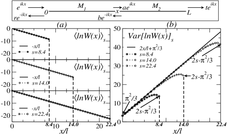
Figure 1: Top panel: the scattering problem for the 1D disordered waveguide of length $L$ described in the text. Lower panels: theoretical results (full lines) and computer simulations (various symbols and dotted lines) for the profiles $\left\langle\ln{\cal W}(x)\right\rangle_{s}$, (panel (a)), and ${\rm var}[\ln{\cal W}(x)]_{s}$, (panel (b)), as functions of $x/\ell$, for three values of $s=L/\ell$. For the variance, Eq. (12) was complemented with Eq. (13) when $x=L$ (see the arrows): their combination accounts for the “bending” shown by the simulation. Agreement is excellent. Simulations consist of $10^{5}$ realizations, with $kd=0.1$ and $k\ell=178$.

Inside the gap, the intensity is

$${\cal W}(x)=|ae^{ikx}+be^{-ikx}|^{2}.$$ (1)

Writing the transfer matrices of the two segments as

$$M_{i}=\left[\begin{array}[]{cc}\alpha_{i}&\beta_{i}\\ \beta_{i}^{*}&\alpha_{i}^{*}\end{array}\right],\;\;\;\;\;i=1,2,$$ (2)

with $|\alpha_{i}|^{2}-|\beta_{i}|^{2}=1$, we satisfy the requirements of time-reversal invariance and flux conservation. When no index $i$ is employed, we refer to the system as a whole. The intensity of Eq. (1), denoted here as ${\cal W}(x;M_{1},M_{2})$, is [mello_genack_et_al_2015, ]

$${\cal W}(x;M_{1},M_{2})=\frac{|\alpha_{2}^{*}e^{ikx}-\beta_{2}^{*}e^{-ikx}|^{2}}{|\alpha_{2}\alpha_{1}+\beta_{2}\beta_{1}^{*}|^{2}}\equiv TF_{x}(M_{2})\;,$$ (3)

where $k$ denotes the wavenumber and $T(M_{1},M_{2})$ the transmission coefficient of the full sample. In the polar decomposition defined in Ref. [mello-kumar, ], the transfer matrices $M_{i}$ can be written in terms of “radial parameters” $\lambda_{i}\geq 0$ [$T_{i}=1/(1+\lambda_{i})$] and two phases, $\theta_{i}$ and $\mu_{i}$, as $\alpha_{i}=\sqrt{1+\lambda_{i}}\exp(i\theta_{i}),\;\;\beta_{i}=\sqrt{\lambda_{i}}\exp(i(2\mu_{i}-\theta_{i}))$. The function $F_{x}(M_{2})$ in Eq. (3) is then

$$F_{x}(M_{2})=A(\lambda_{2})-B(\lambda_{2})\cos 2(\mu_{2}-\theta_{2}+kx)\;,$$ (4)

with $A(\lambda_{2})=1+2\lambda_{2}$ and $B(\lambda_{2})=2\sqrt{\lambda_{2}(1+\lambda_{2})}$.

The above expressions refer to a single configuration of disorder. Assuming the disorder is uncorrelated, quantities associated with the two sections of the sample are statistically independent of one another. The expectation value over an ensemble of configurations of a function $f({\cal W}(x))$ can be computed using the PDF of the transfer matrices for the two sections, $p_{x}(M_{1})$ and $p_{L-x}(M_{2})$. For samples of length $L$, Melnikov’s diffusion equation governs the evolution with $s=L/\ell$ of the marginal PDF $w_{s}(\lambda)$ of the radial parameter $\lambda$ as

$$\frac{\partial w_{s}(\lambda)}{\partial s}=\frac{\partial}{\partial\lambda}\left[\lambda(1+\lambda)\frac{\partial w_{s}(\lambda)}{\partial\lambda}\right]\;.$$ (5)

Equation (5) is solved with the initial condition $w_{s=0}(\lambda)=\delta_{+}(\lambda),$ where $\delta_{+}(\lambda)$ is a one-sided delta function. In what follows, the statistics of each one of the radial parameters $\lambda_{1}$, $\lambda_{2}$ of the two statistically independent sections of the wire will be described by Eq. (5): for the left segment, $s$ will be replaced by $s_{1}=x/\ell$, and for the right segment, by $s_{2}=(L-x)/\ell$.

From Eq. (3), we find for the ensemble average

$$\langle\ln{\cal W}(x)\rangle_{s}=\langle\ln T\rangle_{s}+\langle\ln F_{x}(M_{2})\rangle_{s_{2}}\;.$$ (6)

The first term is given by the well-known expression

$$\langle\ln T\rangle_{s}\equiv\int_{0}^{\infty}\ln Tw_{s}(\lambda)d\lambda.=-\frac{L}{\ell}\;.$$ (7)

From Eq. (4), the second term can be written as

$$\langle\ln F_{x}(M_{2})\rangle_{s_{2}}=\int_{0}^{\infty}d\lambda_{2}\int_{0}^{2\pi}d\theta_{2}w_{s_{2}}(\lambda_{2},\theta_{2})\int_{0}^{2\pi}\frac{d\mu_{2}}{2\pi}$$

$$\times\ln\big{[}A(\lambda_{2})-B(\lambda_{2})\cos(2(\mu_{2}-\theta_{2}+kx))\big{]}=s_{2},$$ (8)

where we used Eq. (4.224.9) of Ref. [gradshteyn, ] to evaluate the angular integral in Eq. (8). The final result is

$$\left\langle\ln{\cal W}(x)\right\rangle_{s}=-\frac{x}{\ell}.$$ (9)

Notice that the $L$ dependence has dropped out from this result. A simple demonstration of this independence for $x=0$ is given in the supplemental material (SM) presented in Ref. [SM_1, ]; it uses the statistics of the reflection amplitude $r$ of Ref. [yepez-jjs, ]. For $x=L$, Eq. (9) reduces to Eq. (7) for the full sample. We may alternatively use the identity (26) of Ref. [Anderson_1980, ], to show the independence of the result on $L$.

From Eq. (3), the second moment of $\ln{\cal W}(x)$ is

$$\left\langle\left[\ln{\cal W}(x)\right]^{2}\right\rangle_{s}= \left\langle(\ln T)^{2}\right\rangle_{s}+\Big{\langle}[\ln F_{x}(M_{2})]^{2}\Big{\rangle}_{s_{2}}$$ (10)

$$+2\Big{\langle}(\ln T)\left[\ln F_{x}(M_{2})\right]\Big{\rangle}_{s,s_{2}}\;.$$

Although we have not succeeded in computing the three terms in Eq. (10) for arbitrary $s=L/\ell$, we have found approximate expressions for the case when the wave in the right segment is localized: $s,s_{2}\gg 1$. We obtain

$$\left\langle(\ln T)^{2}\right\rangle_{s}=s^{2}+2s-2C+\omega_{1}(s),$$ (11a)

$$\Big{\langle}[\ln F_{x}(M_{2})]^{2}\Big{\rangle}_{s_{2}}=s_{2}^{2}+2s_{2}+(\frac{\pi^{2}}{3}-2C)+\omega_{2}(s_{2}),$$ (11b)

$$2\Big{\langle}(\ln T)\left[\ln F_{x}(M_{2})\right]\Big{\rangle}_{s,s_{2}}=-2s_{2}s-4s_{2}+4C+\omega_{3}(s_{2}),$$

(11c)

where [marlos_et_al, ] $C\equiv\int_{0}^{\infty}\langle T\rangle_{s}ds=\pi^{2}/6.$ Collecting terms and using Eq. (9), we find for the variance of $\ln{\cal W}(x)$

$${\rm var}\left[\ln{\cal W}(x)\right]_{s}=2\frac{x}{\ell}+\pi^{2}/3+\omega_{4}(s_{2}),\;\;\;\;s,s_{2}\gg 1.$$ (12)

In Eqs. (11) and (12), $\omega_{i}(s)$ are functions that tend to 0 as $s\to\infty$ (e.g., $\omega_{1}=\int_{0}^{s}\langle T\rangle_{s}ds-\pi^{2}/6$). For $x=L$ we cannot apply the above result, Eq. (12), since this would violate the condition $s_{2}\gg 1$. Since for $x=L$, ${\cal W}(L)=T$, one finds, from Eqs. (11a) and (7)

$$({\rm var}(\ln T))_{s}=2\frac{L}{\ell}-\pi^{2}/3+\omega_{1}(s),\hskip 14.22636pts\gg 1\;.$$ (13)

To leading order in $s\gg 1$, Eq. (13) can be approximated by its first term, which represents the well-known result that the variance of the logarithm of the transmission scales as twice (the absolute value of) its expectation value; in addition, $\ln T$ has a normal probability distribution [mello86, ; beenakker97, ], with $\langle\ln T\rangle=-s$, $({\rm var}(\ln T))_{s}=2s$. The next term in Eq. (13), i.e., $-\pi^{2}/3$, represents a correction to $({\rm var}(\ln T))_{s}$ of order $s^{0}$. To the best of our knowledge, this correction has not been reported before: earlier studies were restricted to lowest order in $s$; this correction may not be negligible if $s$ is not large (see, e.g., Fig. 1(b), explained below).

To check results, we have carried out computer simulations of random waveguides supporting a single propagating mode. These simulations can be applied to both the QM and EM cases: i) in the QM case, the disordered potential is a random function of position; we chose sequences of equidistant barriers (idealized as delta-function potentials), with separation $d$ small compared with the wavelength; ii) in the EM case, it is the index of refraction $n$ appearing in the Helmholtz equation which is a similar random function of position.

The profiles of $\left\langle\ln{\cal W}(x)\right\rangle_{s}$ and ${\rm var}[\ln{\cal W}(x)]_{s}$, Eqs. (9) and (12), are shown, as functions of $x/\ell$, for three values of $s$, in panels (a) and (b) of Fig. 1. The results in (a) show that $\left\langle\ln{\cal W}(x)\right\rangle_{s}$ is insensitive to $s=L/\ell$, while the results in (b) show that ${\rm var}[\ln{\cal W}(x)]_{s}$ is insensitive in the linear regime. Simulations are in excellent agreement with theoretical results. From Eq. (12), the theoretical variance for $x=0$ has the universal value $\pi^{2}/3$ in the localized regime, which agrees with simulation. A simple derivation of this result is given in the SM presented in Ref. [SM_1, ]. The first moment and variance of $\ln{\cal W}(x)$ are shown as functions of $s$ for fixed values of $x/L$ in panels (a) and (b), respectively, of Fig. 1 of the SM of Ref. [SM_1, ]: they continue to the interior of the sample the results at $x=L$ for $\langle\ln T\rangle_{s}$ and ${\rm var}[\ln T]_{s}$.

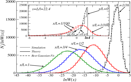
Figure 2: Evolution of the statistical distribution of $\ln{\cal W}(x)$ for $x/L=1.0,\;3/4,\;1/2$ and $1/16$, $x=L$ corresponding to $\ln T$. The histograms are the results of computer simulations with $10^{5}$ realizations each, and $kd=0.1$, $k\ell=178$. All cases are in the localized regime, as $s=L/\ell=22.4$. The ordinate gives the number of events $N_{i}$ falling in box $i$ of the histogram. The continuous curves are Gaussians with the parameters discussed in the text. For $x$ not too close to zero, the agreement between the theoretically constructed Gaussians and the computed generated histograms is excellent.

We have not succeeded in finding the PDF of $\ln{\cal W}(x)$ analytically, but only numerically (Fig. 2): i) When $x$ is not too close to 0, e.g. for $x/L=3/4\;{\rm and}\;1/2$, $\ln{\cal W}(x)$ has a normal PDF with the theoretical centroid and variance given in Eqs. (9) and (12). When $x/L=1$, the PDF is normal, with $\langle\ln{\cal W}(L)\rangle=\langle\ln T\rangle$ and ${\rm var}[\ln{\cal W}(L)]_{s}={\rm var}[\ln T]_{s}$. ii) For $x=0$, unitarity restricts $\ln{\cal W}(0)\leq\ln 4$ (inset in Fig. 2). The PDF cannot be fitted by a truncated Gaussian: the dashed curve is the best “half-Gaussian” fit (with the maximum at $\ln 4$) to the histogram. iii) When $x\neq 0,L$, unitarity imposes no restriction on $\ln{\cal W}(x)$. Close to the left end, $x/L\ll 1$, the PDF of $\ln{\cal W}(x)$ admits non-zero values for $\ln{\cal W}(x)>\ln 4$. iv) For $x/L=1/16$ (body of the figure) and $1/100$ (inset), the dashed curves show the best fit to the histograms by two “half-Gaussians” on either side of the maximum, using two different sets of parameters; however, the left tail is longer than the Gaussian fit.

It is well known that the quantity $\ln T$ of Eqs. (7) and (13) is self averaging [lifshits_et_al-1988, ], whereas $T$ is not. Similarly, when $x\gg\ell$, one can show that $\ln{\cal W}(x)$ of Eqs. (9) and (12) is self averaging, whereas ${\cal W}(x)$, studied in Ref. [mello_genack_et_al_2015, ], is not. This is the main reason for studying $\ln{\cal W}(x)$ in the present paper (see details in the SM of Ref. [SM_1, ]).

We have carried out microwave experiments to explore the statistics of $\ln{\cal W}(x)$ inside random single-mode waveguides. Since $\ln{\cal W}(x)$ self-averages, we are able to obtain sufficient sampling to compare the measurements to theoretical predictions in 100 random configurations. Waves are launched from one end of the waveguide and the signal is detected by an antenna just above a slit along the length of the waveguide. The sample is composed of randomly positioned elements contained within a rectangular copper waveguide, with width and height of 2.286 cm and 1.016 cm, giving a cutoff frequency of 6.56 GHz. The sample is made up of ceramic slabs with dielectric constant $\epsilon=15$, thickness of 0.66 cm covering $93\%$ of the waveguide cross section and U-shaped Teflon elements which are essentially air. The elements in each configuration are randomly selected with equal probability of being either a dielectric or air layer. The air layers may have thicknesses of 1.275, 2.550, or 3.825 cm with equal probability. The incident frequency ranges from 8.50 GHz to 8.59 GHz in $400$ frequency steps. The sample is of length $L$=60 cm. The impact of absorption is removed by Fourier transforming the spectrum into the time domain, multiplying by a factor $\exp({\Gamma_{a}t/2})$ and then transforming back into the frequency domain; $\Gamma_{a}=0.011$ ${\rm ns}^{-1}$ is the decay rate of energy within the sample due to absorption and leakage through the slot along the sample length. It is obtained from the measurement of the linewidth in angular frequency units of the narrowest mode when copper reflectors are placed at the ends of the sample with only a small opening in the reflector on the LHS of the sample to admit energy from the source antenna. Absorbers are placed in the waveguide between the source antenna and the sample input and following the sample output to reduce reflection back into the sample.

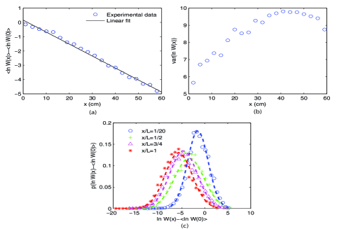
Figure 3: Results from microwave experiments for (a) $\langle\ln{\cal W}(x)\rangle$, (b) ${\rm var}(\ln{\cal W}(x))$. The solid line in (a) shows comparison to the theoretical prediction of a linear fall-off as in Eq. (9). (c) Experimental results for the PDF of $\ln{\cal W}(x)$ at different locations for $s=5$. Lines are Gaussian fit curves.

The experimental results for $\langle\ln{\cal W}(x)\rangle_{s}$ shown in Fig. 3a are well fit by the line $−5.06x/L+0.02$. This linear behavior is in agreement with the fit $s=L/\ell\approx 5$ and $\ell\approx 12$ cm. Results for ${\rm var}[\ln{\cal W}(x)]_{s}$ are shown in Fig. 3b: it increases linearly near the beginning of the sample and bends as $x$ approaches the output boundary, as in the theoretical result of Fig. 1b). However, ${\rm var}[\ln{\cal W}(0)]_{s}\sim 5$ is larger than the predicted value of $\pi^{2}/3=3.29$. This is a consequence of reflection by the source antenna. We find in 1D simulations for a layered sample with an initial layer with a high value of index of refraction $n_{r}$, and hence of reflectivity, that the slope of $\langle\ln{\cal W}(x)\rangle_{s}$ is not affected by reflection from the boundary, but ${\rm var}[\ln{\cal W}(0)]_{s}$ increases with $n_{r}$. The PDF of $\ln{\cal W}(x)$ is shown in Fig. 3c. At the beginning of the sample the distribution is not symmetric; the fit shown in Fig 3c utilizes different Gaussian functions above and below the peak value of the distribution. However, for $x=L/2$ and $x=L$, the PDFs for $\ln{\cal W}(x)$ are Gaussians as seen in Fig. 3c. These results are consistent with features seen in Fig. 2.

In summary, we have used random-matrix theory to calculate the statistics of $\ln{\cal W}(x)$. Since ${\cal W}(L)=T$, SPS corresponds to the particular case $x=L$, in the localized regime $s\gg 1$. More generally, our analysis leads to the correction to SPS of Eq. (13). Extending the MEA into the interior of 1D samples provides a starting point for analyzing the intensity inside systems supporting several open channels.

The authors are indebted to B. Shapiro for valuable suggestions. PAM and AZG wish to thank the Israel Institute of Technology (Haifa, Israel), where part of this work was started, for its hospitality. PAM acknowledges support by DGAPA under contract No. IN109014, and AZG the support of the National Science Foundation under grant No. 1609218 and the help of Noel Evans and Howard Rose for constructing the experimental assembly.

References

- (1) D. J. Thouless, Phys. Rev. Lett. 39, 1167 (1977).
- (2) E. Abrahams, P. Anderson, D. C. Licciardello, and T. V. Ramakrishnan, Phys. Rev. Lett. 42, 673 (1979).
- (3) P. W. Anderson, D. J. Thouless, E. Abrahams, and D. S. Fisher, Phys. Rev. B 22, 3519 (1980).
- (4) V. I. Mel’nikov, Pis’ma Zh. Ekps. Teor. Fiz. 32, 244 (1980) [JETP Lett. 32, 225 (1980)]; Fis. Tverd. Tela (Leningrad) 23, 782 (1981) [Sov. Phys. Solid State 23, 444 (1981)].
- (5) O. N. Dorokhov, Solid State Commun. 51, 381 (1984).
- (6) M. C. W. van Rossum and T. M. Nieuwenhuizen, Rev. Mod. Phys. 71, 313 (1999).
- (7) Z. Shi, J. Wang, and A. Z. Genack, Proc. Nat. Ac. Sc. 111, 2926 (2014).
- (8) O. Dietz, U. Kuhl, H.-J. Stöckmann, N. M. Makarov, and F. M. Izrailev, Phys. Rev. B 83, 134203 (2011).
- (9) Y. L. Gazaryan, Sov. Phys. 29, 996 (1969).
- (10) W. Kohler and G. C. Papanicolau, J. Math. Phys. 14, 1733 (1973).
- (11) P. Neupane and A. G. Yamilov, Phys. Rev. B 92, 014207 (2015).
- (12) B. A. van Tiggelen, A. Lagendijk, and D. S. Wiersma, Phys. Rev. Lett. 84, 4333 (2000); S. E. Skipetrov and B. A. van Tiggelen, Phys. Rev. Lett. 96, 043902 (2006).
- (13) C. Tian, S. Cheung, and Z. Zhang, Phys. Rev. Lett. 105, 263905 (2010).
- (14) I. M. Vellekoop and A. P. Mosk, Phys. Rev. Lett. 101, 120601 (2008).
- (15) S. M. Popoff, G. Lerosey, R. Carminati, M. Fink, A. C. Boccara, and S. Gigan, Phys. Rev. Lett. 104, 100601 (2010).
- (16) W. Choi, A. P. Mosk, Q. Park, and W. Choi, Phys. Rev. B 83, 134207 (2011).
- (17) B. Gérardin, J. Laurent, A. Derode, C. Prada, and A. Aubry, Phys. Rev. Lett. 113, 173901 (2014).
- (18) S. Liew, S. Popoff, A. P. Mosk, W. L. Vos, and H. Cao, Phys. Rev. B 89, 224202 (2014).
- (19) A. G. Yamilov, R. Sarma, B. Redding, B. Payne, H. Noh, and H. Cao, Phys. Rev. Lett. 112, 023904 (2014).
- (20) R. Sarma, A. G. Yamilov, P. Neupane, B. Shapiro, and Hui Cao, Phys. Rev. B 90, 014203 (2014).
- (21) M. Davy, Z. Shi, J. Wang, X. Cheng, and A. Z. Genack, Phys. Rev. Lett. 114, 033901 (2015).
- (22) M. Davy, Z. Shi, J. Park, C. Tian, and A. Z. Genack, Nat. Commun. 6, 6893 (2015).
- (23) R. Sarma, A. G. Yamilov, P. Neupane, and H. Cao, Phys. Rev. B 92, 180203(R) (2015).
- (24) X. Cheng and A. Z. Genack, Opt. Lett. 39, 6324 (2014).
- (25) C. W. J. Beenakker, Rev. Mod. Phys. 69,731 (1997).
- (26) P. A. Mello and N. Kumar, Quantum Transport in Mesoscopic Systems (Oxford University Press, 2010.)
- (27) O. N. Dorokhov, Pis’ma Zh. Eksp. Teor. Fiz., 36, 259 (1982) [JETP Lett., 36, 318 (1982)]
- (28) P. A. Mello, P. Pereyra, and N. Kumar, Ann. Phys. (NY) 181, 290 (1988).
- (29) A. D. Stone, P. A. Mello, K. A. Muttalib, and J.-L. Pichard, Random matrix theory and maximum entropy models for disordered conductors, in Mesoscopic Phenomena in Solids, B.L. Altshuler, P.A. Lee and E. A. Webb, editors, North-Holland, 1991.
- (30) P. A. Mello, Z. Shi, and A. Z. Genack, Physica E 74 603 (2015).
- (31) J. A. Sánchez-Gil and V. Freilikher, Phys. Rev. B 68 075103 (2003)
- (32) I. S. Gradshteyn and I. M. Ryzhik, Table of Integrals, Series, and Products (Academic Press, New York and London, 1965.)
- (33) See Supplemental Material at [URL] for [Insensitivity of to ; the “universal” value of ; self-averaging property of and ].
- (34) M. Yépez and J. J. Sáenz, Europhys. Lett. 108, 17006 (2014).
- (35) P. W. Anderson, D. J. Thouless, E. Abrahams, and D. S. Fisher, Phys. Rev. B 22, 3519 (1980).
- (36) We have not succeeded in finding analytically. Numerical integration (M. Díaz, P. A. Mello, M. Yépez, and S. Tomsovic, Phys. Rev. B 91, 184203 (2015), Eq. (4.7)) gives to 12 decimal places.
- (37) P. A. Mello, J. Math. Phys. 27, 2876 (1986).
- (38) I. M. Lifshits, S. A. Gredeskul, and L. A. Pastur, Introduction to the theory of disordered systems, E. Yankovsky, tr., John Wiley & Sons, New York, 1988, pp. 1, 20; V. D. Freilikher and S. A. Gredeskul, Localization of waves in media with one-dimensional disorder, E. Wolf, ed., Progress in Optics XXX, Elsevier Science publishers B. V., 1992, pp. 145.