Fast Fourier Color Constancy

Abstract

We present Fast Fourier Color Constancy (FFCC), a color constancy algorithm which solves illuminant estimation by reducing it to a spatial localization task on a torus. By operating in the frequency domain, FFCC produces lower error rates than the previous state-of-the-art by $13-20\%$ while being $250-3000\times$ faster. This unconventional approach introduces challenges regarding aliasing, directional statistics, and preconditioning, which we address. By producing a complete posterior distribution over illuminants instead of a single illuminant estimate, FFCC enables better training techniques, an effective temporal smoothing technique, and richer methods for error analysis. Our implementation of FFCC runs at $\sim 700$ frames per second on a mobile device, allowing it to be used as an accurate, real-time, temporally-coherent automatic white balance algorithm.

1 Intro

A fundamental problem in computer vision is that of estimating the underlying world that resulted in some observed image [1, 5]. One subset of this problem is color constancy: estimating the color of the illuminant of the scene and the colors of the objects in the scene viewed under a white light. Despite its apparent simplicity, this problem has yielded a great deal of depth and challenge for both the human vision and computer vision communities [17, 23]. Color constancy is also a practical concern in the camera industry: producing a natural looking photograph without user intervention requires that the illuminant be automatically estimated and discounted, a process referred to as “auto white balance” among practitioners. Though there is a profound historical connection between color constancy and consumer photography (exemplified by Edwin Land, the inventor of both Retinex theory [27] and the Polaroid instant camera), “color constancy” and “white balance” have come to mean different things — color constancy aims to recover the veridical world behind an image, while white balance aims to give an image a pleasant appearance consistent with some aesthetic or cultural norm. But with the current ubiquity of learning-based techniques in computer vision, both problems reduce to just estimating the “best” illuminant from an image, and the question of whether that illuminant is objectively true or subjectively attractive is just a matter of the data used during training.

Despite their accuracy, modern learning-based color constancy algorithms are not immediately suitable as practical white balance algorithms, as practical white balance has several requirements besides accuracy:
Speed - An algorithm running in a camera’s viewfinder must run at $30$ FPS on mobile hardware. But a camera’s compute budget is precious: demosaicing, face detection, auto exposure, etc, must also run simultaneously and in real time. Spending more than a small fraction (say, $5-10\%$) of a camera’s compute budget on white balance is impractical, suggesting that our speed requirement is closer to $1-5$ milliseconds per frame.
Impoverished Input - Most color constancy algorithms are designed for full resolution, high bit-depth input images, but operating on such large images is challenging and costly in practice. To be fast, the algorithm must work well on the small, low bit-depth “preview” images ($32\times 24$ or $64\times 48$ pixels, $8$-bit) which are usually computed by specialized camera hardware for this task.
Uncertainty - In addition to the illuminant, the algorithm should produce some confidence measure or a complete posterior distribution over illuminants, thereby enabling convenient downstream integration with hand-engineered heuristics or external sources of information.
Temporal Coherence - The algorithm should allow the estimated illuminant to be smoothed over time, to prevent color composition in videos from varying erratically.

In this paper we present a novel color constancy algorithm, which we call “Fast Fourier Color Constancy” (FFCC). Viewed as a color constancy algorithm, FFCC is $13-20\%$ more accurate than the state of the art on standard benchmarks. Viewed as a prospective white balance algorithm, FFCC addresses our previously described requirements: Our technique is $250-3000\times$ faster than the state of the art, and is capable of running at $1.44$ milliseconds per frame on a standard consumer mobile platform using the thumbnail images already produced by that camera’s hardware. FFCC produces a complete posterior distribution over illuminants which allows us to reason about uncertainty and enables simple and effective temporal smoothing.

We build on the “Convolutional Color Constancy” (CCC) approach of [4], which is currently one of the top-performing techniques on standard color constancy benchmarks [12, 20, 31]. CCC works by observing that applying a per-channel gain to a linear RGB image is equivalent to inducing a 2D translation of the log-chroma histogram of that image, which allows color constancy to be reduced to the task of localizing a signature in log-chroma histogram space. This reduction is at the core of the success of CCC and, by extension, our FFCC technique; see [4] for a thorough explanation. The primary difference between FFCC is that instead of performing an expensive localization on a large log-chroma plane, we perform a cheap localization on a small log-chroma torus.

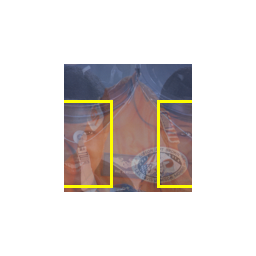
                 (a) Image $A$                                   (b) Aliased Image $B$                 

Figure 1: CCC [4] reduces color constancy to a 2D localization problem similar to object detection (1a). FFCC repeatedly wraps this 2D localization problem around a small torus (1b), which creates challenges but allows for faster illuminant estimation. See the text for details.

At a high level, CCC reduces color constancy to object detection — in the computability theory sense of “reduce”. FFCC reduces color constancy to localization on a torus instead of a plane, and because this task has no intuitive analogue in computer vision we will attempt to provide one. Given a large image $A$ on which we would like to perform object detection, imagine constructing a smaller $n\times n$ image $B$ in which each pixel in $B$ is the sum of all values in $A$ separated by a multiple of $n$ pixels in either dimension:

$$B(i,j)=\sum_{k,l}A(i+nk,j+nl)$$ (1)

This amounts to taking $A$ and repeatedly wrapping it around a small torus (see Figure 1). Detecting objects this way may yield a speedup as the image being processed is smaller, but it also raises new problems: 1) pixel values are corrupted with superimposed shapes that make detection difficult, 2) detections must “wrap” around the edges of this toroidal image, and 3) instead of an absolute, global location we can only recover an aliased, incomplete location. FFCC works by taking the large convolutional problem of CCC (ie, face detection on $A$) and aliasing that problem down to a smaller size where it can be solved efficiently (ie, face detection on $B$). We will show that we can learn an effective color constancy model in the face of the difficulty and ambiguity introduced by aliasing. This convolutional classifier will be implemented and learned using FFTs, because the naturally periodic nature of FFT convolutions resolves the problem of detections “wrapping” around the edge of toroidal images, and produces a significant speedup.

Our approach to color constancy introduces a number of issues. The aforementioned periodic ambiguity resulting from operating on a torus (which we dub “illuminant aliasing”) requires new techniques for recovering a global illuminant estimate from an aliased estimate (Section 3). Localizing the centroid of the illuminant on a torus is difficult, requiring that we adopt and extend techniques from the directional statistics literature (Section 4). But our approach presents a number of benefits. FFCC improves accuracy relative to CCC by $17-24\%$ while retaining its flexibility, and allows us to construct priors over illuminants (Section 5). By learning in the frequency-domain we can construct a novel method for fast frequency-domain regularization and preconditioning, making FFCC training $20\times$ faster than CCC (Section 6). Our model produces a complete unimodal posterior over illuminants as output, allowing us to construct a Kalman filter-like approach for processing videos instead of independent images (Section 7).

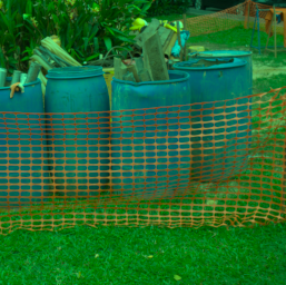
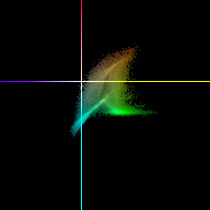
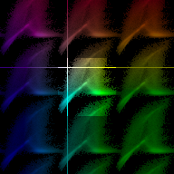
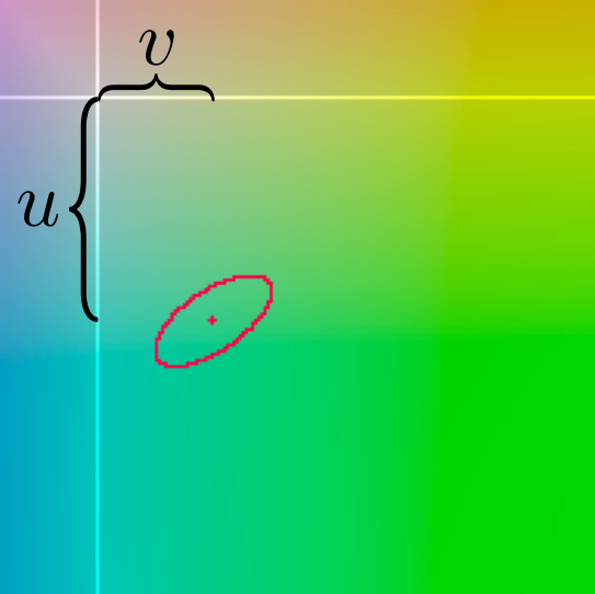
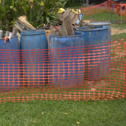
            (a) Input Image                         (b) Histogram                         (c) Aliased Histogram                         (d) Aliased Prediction                              (e) De-aliased Prediction                              (f) Output Image            

Figure 2: An overview of our pipeline demonstrating the problem of illuminant aliasing. Similarly to CCC, we take an input image (2a) and transform it into a log-chroma histogram (2b, presented in the same format as in [4]). But unlike CCC, our histograms are small and toroidal, meaning that pixels can “wrap around” the edges (2c, with the torus “unwrapped” once in every direction). This means that the centroid of a filtered histogram, which would simply be the illuminant estimate in CCC, is instead an infinite family of possible illuminants (2d). This requires de-aliasing, some technique for disambiguating between illuminants to select the single most likely estimate (2e, shown as a point surrounded by an ellipse visualizing the output covariance of our model). Our model’s output $(u,v)$ coordinates in this de-aliased log-chroma space corresponds to the color of the illuminant, which can then be divided into the input image to produce a white balanced image (2f).

2 Convolutional Color Constancy

Let us review the assumptions made in CCC and inherited by our model. Assume that we have a photometrically linear input image $I$ from a camera, with a black level of zero and with no saturated pixels. Each pixel $k$’s RGB value in image $I$ is assumed to be the product of that pixel’s “true” white-balanced RGB value $W^{(k)}$ and some global RGB illumination $L$ shared by all pixels:

$$\forall_{k}\,\,\begin{bmatrix}I_{r}^{(k)}\\ I_{g}^{(k)}\\ I_{b}^{(k)}\end{bmatrix}=\begin{bmatrix}W_{r}^{(k)}\\ W_{g}^{(k)}\\ W_{b}^{(k)}\end{bmatrix}\circ\begin{bmatrix}L_{r}\\ L_{g}\\ L_{b}\end{bmatrix}$$ (2)

The task of color constancy is to use the input image $I$ to estimate $L$, and with that produce $W^{(k)}=I^{(k)}/L$.

Given a pixel from our input RGB image $I^{(k)}$, CCC defines two log-chroma measures:

$$u^{(k)} =\log\left(I^{(k)}_{g}/I^{(k)}_{r}\right) v^{(k)} =\log\left(I^{(k)}_{g}/I^{(k)}_{b}\right)$$ (3)

The absolute scale of $L$ is assumed to be unrecoverable, so estimating $L$ simply requires estimating its log-chroma:

$$L_{u} =\log\left(L_{g}/L_{r}\right) L_{v} =\log\left(L_{g}/L_{b}\right)$$ (4)

After recovering $(L_{u},L_{v})$, assuming that $L$ has a magnitude of $1$ lets us recover the RGB values of the illuminant:

$$L_{r} ={\exp(-L_{u})\over z}\qquad L_{g}={1\over z}\qquad L_{b}={\exp(-L_{v})\over z}$$

$$z =\sqrt{\exp(-L_{u})^{2}+\exp(-L_{v})^{2}+1}$$ (5)

Framing color constancy in terms of predicting log-chroma has several small advantages over the standard RGB approach ($2$ unknowns instead of $3$, better numerical stability, etc) but the primary advantage of this approach is that using log-chroma turns the multiplicative constraint relating $W$ and $I$ into an additive constraint [15], and this in turn enables a convolutional approach to color constancy. As shown in [4], color constancy can be framed as a 2D spatial localization task on a log-chroma histogram $N$, where some sliding-window classifier is used to filter that histogram and the centroid of that filtered histogram is used as the log-chroma of the illuminant.

3 Illuminant Aliasing

We assume the same convolutional premise of CCC, but with one primary difference to improve quality and speed: we use FFTs to perform the convolution that filters the log-chroma histogram, and we use a small histogram to make that convolution as fast as possible. This change may seem trivial, but the periodic nature of FFT convolution combined with the properties of natural images has a significant effect, as we will demonstrate.

Similarly to CCC, given an input image $I$ we construct a histogram $N$ from $I$, where $N(i,j)$ is the number of pixels in $I$ whose log-chroma is near the $(u,v)$ coordinates corresponding to histogram position $(i,j)$:

$$N(i,j)=\displaystyle\sum_{k}\Bigg{(} \operatorname{mod}\left({u^{(k)}-u_{\mathit{lo}}\over h}-i,n\right)<1$$

$$\wedge\,\, \operatorname{mod}\left({v^{(k)}-v_{\mathit{lo}}\over h}-j,n\right)<1\Bigg{)}$$ (6)

Where $i$, $j$ are $0$-indexed, $n=64$ is the number of bins, $h=1/32$ is the bin size, and $(u_{\mathit{lo}},v_{\mathit{lo}})$ is the starting point of the histogram. Because our histogram is too small to contain the wide spread of colors present in most natural images, we use modular arithmetic to cause pixels to “wrap around” with respect to log-chroma (any other standard boundary condition would violate our convolutional assumption and would cause many image pixels to be ignored). This means that, unlike standard CCC, a single $(i,j)$ coordinate in the histogram no longer corresponds to an absolute $(u,v)$ color, but instead corresponds to an infinite family of $(u,v)$ colors. Accordingly, the centroid of a filtered histogram no longer corresponds to the color of the illuminant, but instead is an infinite set of illuminants. We will refer to this phenomenon as illuminant aliasing. Solving this problem requires that we use some technique to de-alias an aliased illuminant estimate. A high-level outline of our FFCC pipeline that illustrates illuminant (de-)aliasing can be seen in Fig. 2.

De-aliasing requires that we use some external information (or some external color constancy algorithm) to disambiguate between illuminants. An intuitive approach is to select the illuminant that causes the average image color to be as neutral as possible, which we call “gray world de-aliasing”. We compute average log-chroma values $(\bar{u},\bar{v})$ for the entire image and use this to turn an aliased illuminant estimate $(\hat{L}_{u},\hat{L}_{v})$ into a de-aliased illuminant $(\hat{L}^{\prime}_{u},\hat{L}^{\prime}_{v})$:

$$\bar{u}=\operatorname{mean}_{k}\left(u^{(k)}\right)\quad\quad\bar{v}=\operatorname{mean}_{k}\left(v^{(k)}\right)$$ (7)

$$\begin{bmatrix}\hat{L}^{\prime}_{u}\\ \hat{L}^{\prime}_{v}\end{bmatrix}=\begin{bmatrix}\hat{L}_{u}\\ \hat{L}_{v}\end{bmatrix}-(nh)\left\lfloor{1\over nh}\begin{bmatrix}\hat{L}_{u}-\bar{u}\\ \hat{L}_{v}-\bar{v}\end{bmatrix}+{1\over 2}\right\rfloor$$ (8)

Another approach, which we call “gray light de-aliasing”, is to assume that the illuminant is as close to the center of the histogram as possible. This de-aliasing approach simply requires carefully setting the starting point of the histogram $(u_{\mathit{lo}},v_{\mathit{lo}})$ such that the true illuminants in natural scenes all lie within the span of the histogram, and setting $\hat{L}^{\prime}=\hat{L}$. We do this by setting $u_{\mathit{lo}}$ and $v_{\mathit{lo}}$ to maximize the distance between the edges of the histogram and the bounding box surrounding the ground-truth illuminants in the training data. Gray light de-aliasing is trivial to implement but, unlike gray world de-aliasing, it will systematically fail if the histogram is too small to fit all illuminants within its span.

To summarize the difference between CCC [4] and our approach with regards to illuminant aliasing, CCC (approximately) performs illuminant estimation as follows:

$$\begin{bmatrix}\hat{L}_{u}\\ \hat{L}_{v}\end{bmatrix}=\begin{bmatrix}u_{\mathit{lo}}\\ v_{\mathit{lo}}\end{bmatrix}+h\left(\operatorname*{arg\,max}_{i,j}\left(N*F\right)\right)$$ (9)

Where $N*F$ is performed using a pyramid convolution. FFCC corresponds to this procedure:

$$P \leftarrow\operatorname{softmax}\left(N*F\right)$$ (10)

$$(\boldsymbol{\mu},\boldsymbol{\Sigma}) \leftarrow\operatorname{fit\_bvm}(P)$$ (11)

$$\begin{bmatrix}\hat{L}_{u}\\ \hat{L}_{v}\end{bmatrix} \leftarrow\operatorname{de\_alias}(\boldsymbol{\mu})$$ (12)

Where $N$ is a small and aliased toroidal histogram, convolution is performed with FFTs, and the centroid of the filtered histogram is estimated and de-aliased as necessary. By constructing this pipeline to be differentiable we can train our model in an end-to-end fashion by propagating the gradients of some loss computed on the de-aliased illuminant prediction $\hat{L}$ back onto the learned filters $F$. The centroid fitting in Eq. 11 is performed by fitting a bivariate von Mises distribution to a PDF, which we will now explain.

4 Differentiable Bivariate von Mises

Our architecture requires some mechanism for reducing a toroidal PDF $P(i,j)$ to a single estimate of the illuminant. Localizing the center of mass of a histogram defined on a torus is difficult: fitting a bivariate Gaussian may fail when the input distribution “wraps around” the sides of the PDF, as shown in Fig. 3. Additionally, for the sake of temporal smoothing (Section 7) and confidence estimation, we want our model to predict a well-calibrated covariance matrix around the center of mass of $P$. This requires that our model be trained end-to-end, which therefore requires that our mean/covariance fitting be analytically differentiable and therefore usable as a “layer” in our learning architecture. To address these problems we present a variant of the bivariate von Mises distribution [28], which we will use to efficiently localize the mean and covariance of $P$ in a manner that allows for easy backpropagation.

The bivariate von Mises distribution (BVM) is a common parameterization of a PDF on a torus. There exist several parametrizations which mostly differ in how “concentration” is represented (“concentration” having a similar meaning to covariance). All of these parametrizations present problems in our use case: none have closed form expressions for maximum likelihood estimators [24], none lend themselves to convenient backpropagation, and all define concentration in terms of angles and therefore require “conversion” to covariance matrices during color de-aliasing. For these reasons we present an alternative parametrization in which we directly estimate a BVM as a mean $\boldsymbol{\mu}$ and covariance $\boldsymbol{\Sigma}$ in a simple and differentiable closed form expression. Though necessarily approximate, our estimator is accurate when the distribution is well-concentrated, which is generally the case for our task.

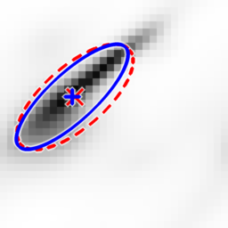
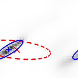
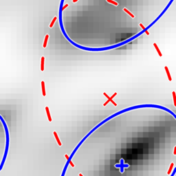
Figure 3: We fit a bivariate von Mises distribution (shown in solid blue) to toroidal PDFs $P(i,j)$ to produce an aliased illuminant estimate. Contrast this with fitting a bivariate Gaussian (shown in dashed red) which treats the PDF as if it lies on a plane. Both approaches behave similarly if the distribution lies near the center of the unwrapped plane (left) but fitting a Gaussian fails as the distribution begins to “wrap around” the edge (middle, right).

Our input is a PDF $P(i,j)$ of size $n\times n$, where $i$ and $j$ are integers in $[0,n-1]$. For convenience we define a mapping from $i$ or $j$ to angles in $[0,2\pi)$ and the marginal distributions of $P$ with respect to $i$ and $j$:

$$\theta(i)={2\pi i\over n}\quad\,\,P_{i}(i)=\sum_{j}P(i,j)\quad\,\,P_{j}(j)=\sum_{i}P(i,j)$$

We also define the marginal expectation of the sine and cosine of the angle:

$$y_{i}=\sum_{i}P_{i}(i)\sin(\theta(i))\quad x_{i}=\sum_{i}P_{i}(i)\cos(\theta(i))$$ (13)

With $x_{j}$ and $y_{j}$ defined similarly.

Estimating the mean $\boldsymbol{\mu}$ of a BVM from a histogram just requires computing the circular mean in $i$ and $j$:

$$\boldsymbol{\mu}=\begin{bmatrix}u_{\mathit{lo}}\\ v_{\mathit{lo}}\end{bmatrix}+h\begin{bmatrix}\operatorname{mod}\left({n\over 2\pi}\operatorname{atan2}(y_{i},x_{i}),n\right)\\ \operatorname{mod}\left({n\over 2\pi}\operatorname{atan2}(y_{j},x_{j}),n\right)\\ \end{bmatrix}$$ (14)

Eq. 14 includes gray light de-aliasing, though gray world de-aliasing can also be applied to $\boldsymbol{\mu}$ after fitting.

We can fit the covariance of our model by simply “unwrapping” the coordinates of the histogram relative to the estimated mean and treating these unwrapped coordinates as though we are fitting a bivariate Gaussian. We define the “unwrapped” $(i,j)$ coordinates such that the “wrap around” point on the torus lies as far away from the mean as possible, or equivalently, such that the unwrapped coordinates are as close to the mean as possible:

$$\bar{i} =\operatorname{mod}\left(i-\left\lfloor\boldsymbol{\mu}_{u}-u_{\mathit{lo}}\over h\right\rfloor+{n\over 2},n\right)$$

$$\bar{j} =\operatorname{mod}\left(j-\left\lfloor\boldsymbol{\mu}_{v}-v_{\mathit{lo}}\over h\right\rfloor+{n\over 2},n\right)$$ (15)

Our estimated covariance matrix is simply the sample covariance of $P(\bar{i},\bar{j})$:

$$\operatorname{E}\left[\bar{i}\right]=\sum_{i}P_{i}(i)\bar{i}\quad\quad\displaystyle\operatorname{E}\left[\bar{j}\right]=\sum_{j}P_{j}(j)\bar{j}$$ (16)

We regularize the sample covariance matrix slightly by adding a constant $\epsilon=1$ to the diagonal.

With our estimated mean and covariance we can compute our loss: the negative log-likelihood of a Gaussian (ignoring scale factors and constants) relative to the true illuminant $L^{*}$:

Using this loss causes our model to produce a well-calibrated complete posterior of the illuminant instead of just a single estimate. This posterior will be useful when processing video sequences (Section 7) and also allows us to attach confidence estimates to our predictions using the entropy of $\boldsymbol{\Sigma}$ (see the appendix).

Our entire system is trained end-to-end, which requires that every step in BVM fitting and loss computation be analytically differentiable. See the appendix for the analytical gradients for Eqs. 14, 17, and 18, which can be chained together to backpropagate the gradient of $f\left(\cdot\right)$ onto the input PDF $P$.

5 Model Extensions

The system we have described thus far (compute a periodic histogram of each pixel’s log-chroma, apply a learned FFT convolution, apply a softmax, fit a de-aliased bivariate von Mises distribution) works reasonably well (Model A in Table 8) but does not produce state-of-the-art results. This is likely because this model reasons about pixels independently, ignores all spatial information in the image, and does not consider the absolute color of the illuminant. Here we present extensions to the model which address these issues and improve accuracy accordingly.

As explored in [4], a CCC-like model can be generalized to a set of “augmented” images provided that these images are non-negative and “scale with intensity” [14]. This lets us apply certain filtering operations to image $I$ and, instead of constructing a single histogram from our image, construct a “stack” of histograms constructed from the image and its filtered versions. Instead of learning and applying one filter, we learn a stack of filters and sum across channels after convolution. The general family of augmented images used in [4] are expensive to compute, so we instead use just the input image $I$ and a local measure of absolute deviation in the input image:

These two features appears to perform similarly to the four features used in [4], while being cheaper to compute.

Just as a sliding-window object detector is often invariant to the absolute location of an object in an image, the convolutional nature of our baseline model makes it invariant to any global shift of the color of the input image. This means that our baseline model cannot rely on any statistical regularities of the illumination by, say, modeling black body radiation, the specific properties of commonly manufactured light bulbs, or any varying spectral sensitivity across cameras. Though CCC does not model illumination directly, it appears to indirectly reason about illumination by using the boundary conditions of its pyramid convolution to learn a model which is not truly spatially varying and is therefore sensitive to absolute color. Because a torus has no boundaries, our model is invariant to global input color, so we must therefore introduce a mechanism for directly reasoning about illuminants. We use a per-illuminant “gain” map $G(i,j)$ and “bias” map $B(i,j)$, which together apply a per-illuminant affine transformation to the output of our previously-described convolution at (aliased) color $(i,j)$. The bias $B$ causes our model to prefer certain illuminants over others, while the gain $G$ causes the contribution of the convolution at certain colors to be amplified.

Our two extensions (an augmented edge channel and an illuminant gain/bias map) let us redefine the $P$ in Eq. 10 as

$$P=\operatorname{softmax}\left(B+G\circ\sum_{k}\left(N_{k}*F_{k}\right)\right)$$ (20)

Where $\{F_{k}\}$ are the set of learned filters for each augmented channel’s histogram $N_{k}$, $G$ is our learned gain map, and $B$ is our learned bias map. In practice we actually parametrize $G_{\log}$ when training and define $G=\exp(G_{\log})$, which constraints $G$ to be non-negative. Visualizations of $G$ and $B$ and our learned filters can be seen in Fig. 4.

                    (a) Pixel Filter                                          (b) Edge Filter                                             (c) Illum. Gain                                                (d) Illum. Bias                        

Figure 4: A complete learned model (Model J in Table 8) shown in centered $(u,v)$ log-chroma space, with brightness indicating larger values. Our learned filters are centered around the origin (the predicted white point) and our illuminant gain and bias maps model the black body curve and varying camera sensitivity as two wrap-around line segments (this dataset consists of images from two different cameras).

6 Fourier Regularization and Preconditioning

Our learned model weights $(\{F_{k}\},G,B)$ are all periodic $n\times n$ images. To improve generalization, we want these weights to be small and smooth. In this section we present the general form of the regularization used during training, and we show how this regularization lets us precondition the optimization problem solved during training to find lower-cost minima in fewer iterations. Because this frequency-domain optimization technique applies generally to any optimization problem concerning smooth and periodic images, we will describe it in general terms.

Let us construct an optimization problem with respect to a single $n\times n$ image $Z$ consisting of a data term $f(Z)$ and a regularization term $g(Z)$:

$$Z^{*}=\operatorname*{arg\,min}_{Z}\left(f\left(Z\right)+g\left(Z\right)\right)$$ (21)

We require that the regularization $g(Z)$ is the weighted sum of squared periodic convolutions of $Z$ with some filter bank. In our experiments $g(Z)$ is the weighted sum of the squared difference between adjacent values (similar to a total variation loss [30]) and the sum of squared values:

$$g(Z)=\textstyle \lambda_{1}\textstyle\sum_{i,j}\big{(}\left(Z\left(i,j\right)-Z\left(\operatorname{mod}(i+1,n),j\right)\right)^{2}$$

$$\quad\quad\,\,\,\,+\left(Z\left(i,j\right)-Z\left(i,\operatorname{mod}(j+1,n)\right)\right)^{2}\big{)}$$

$$+ \lambda_{0}\textstyle\sum_{i,j}Z(i,j)^{2}$$ (22)

Where $\lambda_{1}$ and $\lambda_{0}$ are hyperparameters that determine the strength of each smoothness term. We require that $\lambda_{0}>0$ to prevent divide-by-zero issues during preconditioning.

We use a variant of the standard FFT $\mathcal{F}_{\mathrm{v}}\left(\cdot\right)$ which bijectively maps from some real $n\times n$ image to a real $n^{2}$-dimensional vector, instead of the complex $n\times n$ image produced by a standard FFT (See the appendix for a formal description). With this, we can rewrite Eq. 22 as follows:

$$\mathbf{w}={1\over n}\sqrt{\lambda_{1}\left(\lvert\mathcal{F}_{\mathrm{v}}\left([1,-1]\right)\rvert^{2}+\lvert\mathcal{F}_{\mathrm{v}}\left([1;-1]\right)\rvert^{2}\right)+\lambda_{0}}$$

$$g(Z)=\mathcal{F}_{\mathrm{v}}\left(Z\right)^{\mathrm{T}}\operatorname{diag}\left(\mathbf{w}\right)^{2}\mathcal{F}_{\mathrm{v}}\left(Z\right)$$ (23)

where the vector $\mathbf{w}$ is just some fixed function of the definition of $g(Z)$ and the values of the hyperparameters $\lambda_{1}$ and $\lambda_{0}$. The 2-tap difference filters in $\mathcal{F}_{\mathrm{v}}\left([1,-1]\right)$ and $\mathcal{F}_{\mathrm{v}}\left([1;-1]\right)$ are padded to size $(n\times n)$ before the FFT. With $\mathbf{w}$ we can define a mapping between our 2D image space and a rescaled FFT vector space:

$$\mathbf{z}=\mathbf{w}\circ\mathcal{F}_{\mathrm{v}}\left(Z\right)$$ (24)

Where $\circ$ is an element-wise product. This mapping lets us rewrite the optimization problem in Eq. 21 as:

where $\mathcal{F}^{-1}_{\mathrm{v}}\left(\cdot\right)$ is the inverse of $\mathcal{F}_{\mathrm{v}}\left(\cdot\right)$, and division is element-wise. This reparametrization reduces the complicated regularization of $Z$ to a simple L2 regularization of $\mathbf{z}$, which has a preconditioning effect.

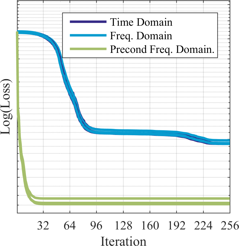
                      Logistic Loss                                             BVM Loss                      

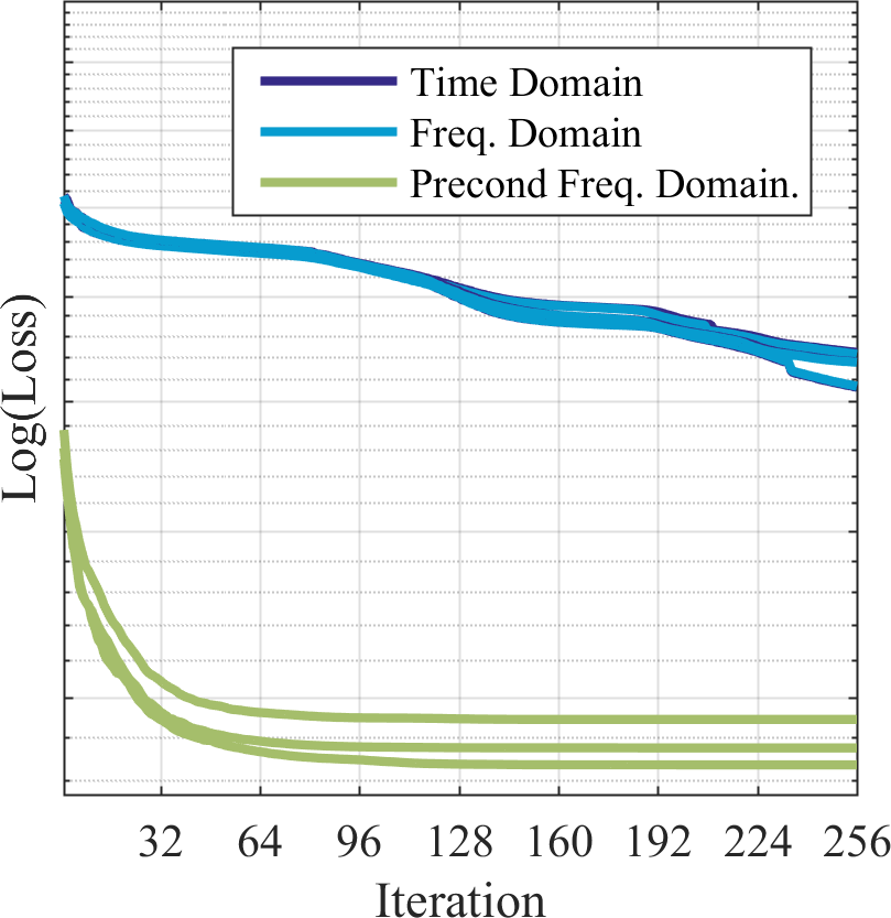
Figure 5: Loss traces for our two stages of training, for three fold cross validation (each line represents a fold) on the Gehler-Shi dataset using LBFGS. Our preconditioned frequency domain optimization produces lower minima at greater rates than are achieved by non-preconditioned optimization in the frequency domain or naive optimization in the time domain.

We use this technique during training to reparameterize all model components $(\{F_{k}\},G,B)$ as rescaled FFT vectors, each with their own values for $\lambda_{0}$ and $\lambda_{1}$. The effect of this can be seen in Fig. 5, where we show the loss during our two training stages. We compare against naive time-domain optimization (Eq. 21) and non-preconditioned frequency-domain optimization (Eq. 25 with $\mathbf{w}=1$). Our preconditioned reformulation exhibits a significant speedup and finds minima with lower losses.

For all experiments (excluding our “deep” variants, see the appendix), training is as follows: All model parameters are initialized to $0$, then we have a convex pre-training step which optimizes Eq. 25 where $f(\cdot)$ is a logistic loss (described in the appendix) using LBFGS for $16$ iterations, and then we optimize Eq. 25 where $f(\cdot)$ is the non-convex BVM loss in Eq. 18 using LBFGS for $64$ iterations.

7 Temporal Smoothing

Color constancy is usually studied in the context of individual images, which are assumed to be IID. But a practical white balance algorithm must run on a video sequence, and must enforce some temporal smoothing of the predicted illuminant to avoid presenting the viewer with an erratically-varying image in the viewfinder. This smoothing cannot be too aggressive or else the viewfinder may appear unresponsive when the illumination changes rapidly (a colorful light turning on, the camera quickly moving outdoors, etc). Additionally, when faced with multiple valid hypotheses (a blue wall under white light vs a white wall under blue light, etc) we may want to use earlier images to resolve ambiguities. These desiderata of stability, responsiveness, and robustness are at odds with each other, and so some compromise must be struck.

Our task of constructing a temporally coherent illuminant estimate is aided by the probabilistic nature of the output of our per-frame model, which produces a posterior distribution over illuminants parametrized as a bivariate Gaussian. Let us assume that we have some ongoing estimate of the illuminant and its covariance $(\boldsymbol{\mu}_{t},\boldsymbol{\Sigma}_{t})$. Given the observed mean and covariance $(\boldsymbol{\mu}_{o},\boldsymbol{\Sigma}_{o})$ provided by our model we update our ongoing estimate by first convolving it with an zero-mean isotropic Gaussian (encoding our prior belief that the illuminant may change over time) and then multiplying that “fuzzed” Gaussian by the observed Gaussian:

$$\boldsymbol{\Sigma}_{t+1} =\left(\left(\boldsymbol{\Sigma}_{t}+\begin{bmatrix}\alpha&0\\ 0&\alpha\end{bmatrix}\right)^{-1}+\boldsymbol{\Sigma}_{o}\right)^{-1}$$ (26)

$$\boldsymbol{\mu}_{t+1} =\boldsymbol{\Sigma}_{t+1}\left(\left(\boldsymbol{\Sigma}_{t}+\begin{bmatrix}\alpha&0\\ 0&\alpha\end{bmatrix}\right)^{-1}\boldsymbol{\mu}_{t}+\boldsymbol{\Sigma}_{o}\boldsymbol{\mu}_{o}\right)^{-1}$$

Where $\alpha$ is a parameter that defines the expected variance of the illuminant over time. This update resembles a Kalman filter but with a simplified transition model, no control model, and variable observation noise.

This temporal smoothing is not used in our benchmarks, but its effect can be seen in the supplemental video.

8 Results

We evaluate our technique using two standard color constancy datasets: the Gehler-Shi dataset [20, 31] and the Cheng et al. dataset [12] (see Tables 8 and 8). For the Gehler-Shi dataset we present several ablations and variants of our model to show the effect of each design decision and to investigate trade-offs between speed and accuracy. Models labeled “full” were run on $384\times 256$ $16$-bit images, while models labeled “thumb” were run on $48\times 32$ $8$-bit images, which are the kind of images that a practical white-balance system embedded on a hardware device might use. Models labeled “4 channel” use the four feature channels used in [4], while models labeled “2 channel” use the two channels we present in Section 5. We also present models in which we only use the “pixel channel” $I$ or the “edge channel” $E$ as input. All models have a histogram size of $n=64$ except for Models K and L where $n$ is varied to show the impact of illuminant aliasing. Two models use “gray world” de-aliasing, and the rest use “gray light” de-aliasing. The former seems slightly less effective than the latter unless chroma histograms are heavily aliased, which is why we use it in Model K. Model C only has one training stage that minimizes logistic loss for $64$ iterations, thereby removing the BVM fitting from training. Model E fixes $G(i,j)=1$ and $B(i,j)=0$, thereby removing the model’s ability to reason about the absolute color of the illuminant. Model B was trained only to minimize the data term (ie, $\lambda_{0}=\lambda_{1}=0$ in Eq. 22) while Model D uses L2 regularization but not total variation (ie, $\lambda_{1}=0$ in Eq. 22). Models N, O and P are variants of Model J in which, instead of learning a fixed model $(\{F_{k}\},G,B)$ we express those model parameters as the output of a small 2-layer neural network. As inputs to this network we use image metadata, which allows the model to reason about exposure time and camera sensor type, and/or a CNN-produced feature vector [35], which allows the model to reason about semantics (see the appendix for details). For each experiment we tune all $\lambda$ hyperparameters to minimize the “average” error during cross-validation, using cyclic coordinate descent.

Model P achieves the lowest-error results, with a $20\%$ reduction in error on Gehler-Shi compared to the previously best-performing published technique. This improvement in accuracy also comes with a significant speedup compared to previous techniques: $\sim\!30$ ms/image for most models, compared to the $520$ ms of CCC [4] or the $3$ seconds (on a GPU) of Shi et al. [32]. Model Q (our fastest model) has an accuracy comparable to [4] and [32] but takes only $1.1$ milliseconds to process an image, making it hundreds or millions of times faster than the current state-of-the art. Additionally, our model appears to be faster to train than the state-of-the-art, though training times for prior work are often not available. All runtimes in Table 8 for our model were computed on an Intel Xeon CPU E5-2680. Runtimes for the “full” model were produced using a Matlab implementation, while runtimes for the “thumb” model were produced using a Halide [29] CPU implementation (our Matlab implementation of Model Q takes $2.37$ ms/image). Runtimes for our “+semantic” models are not presented as we were unable to profile [35] accurately (CNN feature computation appears to dominate runtime).

To demonstrate that our model is a viable automatic white balance system for consumer photography, we ran our Halide code on a 2016 Google Pixel XL using the thumbnail images computed by the device’s camera stack. This implementation ran at $1.44$ms per image, which is equivalent to $30$ frames per second using $<5\%$ of the total compute budget, thereby satisfying our previously-stated speed requirements. A video of our system running in real-time on a phone can be found in the supplement.

Algorithm	Mean	Med.	Tri.	Best	Worst	Avg.	Test	Train
				25%	25%		Time	Time
Support Vector Regression [18]	$8.08$	$6.73$	$7.19$	$3.35$	$14.89$	$7.21$	-	-
White-Patch [8]	$7.55$	$5.68$	$6.35$	$1.45$	$16.12$	$5.76$	$0.16$	-
Grey-world [9]	$6.36$	$6.28$	$6.28$	$2.33$	$10.58$	$5.73$	$0.15$	-
Edge-based Gamut [22]	$6.52$	$5.04$	$5.43$	$1.90$	$13.58$	$5.40$	$3.6$	$1986$
1st-order Gray-Edge [33]	$5.33$	$4.52$	$4.73$	$1.86$	$10.03$	$4.63$	$1.1$	-
2nd-order Gray-Edge [33]	$5.13$	$4.44$	$4.62$	$2.11$	$9.26$	$4.60$	$1.3$	-
Shades-of-Gray [16]	$4.93$	$4.01$	$4.23$	$1.14$	$10.20$	$3.96$	$0.47$	-
Bayesian [20]	$4.82$	$3.46$	$3.88$	$1.26$	$10.49$	$3.86$	$97$	$764$
Yang et al. 2015 [36]	$4.60$	$3.10$	-	-	-	-	$0.88$	-
General Gray-World [3]	$4.66$	$3.48$	$3.81$	$1.00$	$10.09$	$3.62$	$0.91$	-
Natural Image Statistics [21]	$4.19$	$3.13$	$3.45$	$1.00$	$9.22$	$3.34$	$1.5$	$10749$
CART-based Combination [6]	$3.90$	$2.91$	$3.21$	$1.02$	$8.27$	$3.14$	-	-
Spatio-spectral Statistics [11]	$3.59$	$2.96$	$3.10$	$0.95$	$7.61$	$2.99$	$6.9$	$3159$
LSRS [19]	$3.31$	$2.80$	$2.87$	$1.14$	$6.39$	$2.87$	$2.6$	$1345$
Interesection-based Gamut [22]	$4.20$	$2.39$	$2.93$	$0.51$	$10.70$	$2.76$	-	-
Pixels-based Gamut [22]	$4.20$	$2.33$	$2.91$	$0.50$	$10.72$	$2.73$	-	-
Bottom-up+Top-down [34]	$3.48$	$2.47$	$2.61$	$0.84$	$8.01$	$2.73$	-	-
Cheng et al. 2014 [12]	$3.52$	$2.14$	$2.47$	$0.50$	$8.74$	$2.41$	$0.24$	-
Exemplar-based [26]	$2.89$	$2.27$	$2.42$	$0.82$	$5.97$	$2.39$	-	-
Bianco et al. 2015 [7]	$2.63$	$1.98$	-	-	-	-	-	-
Corrected-Moment [14]	$2.86$	$2.04$	$2.22$	$0.70$	$6.34$	$2.25$	$0.77$	$584$
Chakrabarti et al. 2015 [10]	$2.56$	$1.67$	$1.89$	$0.52$	$6.07$	$1.91$	$0.30$	-
Cheng et al. 2015 [13]	$2.42$	$1.65$	$1.75$	$0.38$	$5.87$	$1.73$	$0.25$	$245$
CCC [4]	$1.95$	$1.22$	$1.38$	$0.35$	$4.76$	$1.40$	$0.52$	$2168$
Shi et al. 2016 [32]	$1.90$	$1.12$	$1.33$	$0.31$	$4.84$	$1.34$	$3.0$	-
A) FFCC - full, pixel channel only, no illum.	$2.88$	$1.90$	$2.05$	$0.50$	$6.98$	$2.08$	$0.0076$	$117$
B) FFCC - full 2 channels, no regularization	$2.34$	$1.33$	$1.55$	$0.51$	$5.84$	$1.70$	$0.031$	$96$
C) FFCC - full 2 channels, no BVM loss	$2.16$	$1.45$	$1.56$	$0.76$	$4.84$	$1.78$	$0.031$	$62$
D) FFCC - full 2 channels, no total variation	$1.92$	$1.11$	$1.27$	$0.28$	$4.89$	$1.30$	$0.028$	$104$
E) FFCC - full, 2 channels, no illuminant	$2.14$	$1.34$	$1.52$	$0.37$	$5.27$	$1.53$	$0.031$	$94$
F) FFCC - full, pixel channel only	$2.15$	$1.33$	$1.51$	$0.34$	$5.35$	$1.51$	$0.0063$	$67$
G) FFCC - full, edge channel only	$2.02$	$1.25$	$1.39$	$0.34$	$5.11$	$1.44$	$0.026$	$94$
H) FFCC - full, 2 channels, no precond.	$2.91$	$1.99$	$2.23$	$0.57$	$6.74$	$2.18$	$0.025$	$152$
I) FFCC - full, 2 channels, gray world	$1.79$	$1.01$	$1.22$	$0.29$	$4.54$	$1.24$	$0.029$	$98$
J) FFCC - full, 2 channels	$1.80$	$0.95$	$1.18$	$0.27$	$4.65$	$1.20$	$0.029$	$98$
K) FFCC - full, 4 channels, $n=32$, gray world	$2.69$	$1.31$	$1.49$	$0.37$	$7.48$	$1.70$	$0.068$	$138$
L) FFCC - full, 4 channels, $n=256$	$1.78$	$1.05$	$1.19$	$0.27$	$4.46$	$1.22$	$0.068$	$395$
M) FFCC - full, 4 channels	$1.78$	$0.96$	$1.14$	$0.29$	$4.62$	$1.21$	$0.070$	$96$
N) FFCC - full, 2 channels, +semantics[35]	$1.67$	$0.96$	$1.13$	$0.26$	$4.23$	$1.15$	-	-
O) FFCC - full, 2 channels, +metadata	$1.65$	$0.86$	$1.07$	$0.24$	$4.44$	$1.10$	$0.036$	$143$
P) FFCC - full, 2 channels, +metadata +semantics[35]	$1.61$	$0.86$	$1.02$	$0.23$	$4.27$	$1.07$	-	-
Q) FFCC - thumb, 2 channels	$2.01$	$1.13$	$1.38$	$0.30$	$5.14$	$1.37$	$0.0011$

Table 1: Performance on the Gehler-Shi dataset [20, 31]. We present five error metrics and their average (the geometric mean) with the lowest error per metric highlighted in yellow. We present the time (in seconds) for training each model and for evaluating a single image, when available.

Algorithm	Mean	Med.	Tri.	Best	Worst	Avg.
				25%	25%
White-Patch [8]	$9.91$	$7.44$	$8.78$	$1.44$	$21.27$	$7.24$
Pixels-based Gamut [22]	$5.27$	$4.26$	$4.45$	$1.28$	$11.16$	$4.27$
Grey-world [9]	$4.59$	$3.46$	$3.81$	$1.16$	$9.85$	$3.70$
Edge-based Gamut [22]	$4.40$	$3.30$	$3.45$	$0.99$	$9.83$	$3.45$
Shades-of-Gray [16]	$3.67$	$2.94$	$3.03$	$0.98$	$7.75$	$3.01$
Natural Image Statistics [21]	$3.45$	$2.88$	$2.95$	$0.83$	$7.18$	$2.81$
Local Surface Reflectance Statistics [19]	$3.45$	$2.51$	$2.70$	$0.98$	$7.32$	$2.79$
2nd-order Gray-Edge [33]	$3.36$	$2.70$	$2.80$	$0.89$	$7.14$	$2.76$
1st-order Gray-Edge [33]	$3.35$	$2.58$	$2.76$	$0.79$	$7.18$	$2.67$
Bayesian [20]	$3.50$	$2.36$	$2.57$	$0.78$	$8.02$	$2.66$
General Gray-World [3]	$3.20$	$2.56$	$2.68$	$0.85$	$6.68$	$2.63$
Spatio-spectral Statistics [11]	$3.06$	$2.58$	$2.74$	$0.87$	$6.17$	$2.59$
Bright-and-dark Colors PCA [12]	$2.93$	$2.33$	$2.42$	$0.78$	$6.13$	$2.40$
Corrected-Moment [14]	$2.95$	$2.05$	$2.16$	$0.59$	$6.89$	$2.21$
Color Dog [2]	$2.83$	$1.77$	$2.03$	$0.48$	$7.04$	$2.03$
Shi et al. 2016 [32]	$2.24$	$1.46$	$1.68$	$0.48$	$6.08$	$1.74$
CCC [4]	$2.38$	$1.48$	$1.69$	$0.45$	$5.85$	$1.74$
Cheng 2015 [13]	$2.18$	$1.48$	$1.64$	$0.46$	$5.03$	$1.65$
M) FFCC - full, 4 channels	$1.99$	$1.31$	$1.43$	$0.35$	$4.75$	$1.44$
Q) FFCC - thumb, 2 channels	$2.06$	$1.39$	$1.53$	$0.39$	$4.80$

Table 2: Performance on the dataset from Cheng et al.Cheng14, in the same format as Table 8, excluding runtimes. As was done in [4] we present the average performance (the geometric mean) over all $8$ cameras in the dataset.

9 Conclusion

We have presented FFCC, a color constancy algorithm that produces a $13-20\%$ reduction in error and a $250-3000\times$ speedup relative to prior work. In doing so we have introduced the concept of convolutional color constancy on a torus, and we have introduced techniques for illuminant de-aliasing and differentiable bivariate von Mises fitting required for this toroidal approach. We have also presented a novel technique for fast Fourier-domain optimization subject to a certain family of regularizers. FFCC produces a complete posterior distribution over illuminants, which lets us assess the model’s confidence and also enables a Kalman filter-like temporal smoothing model. FFCC’s speed, accuracy, and temporal consistency allows it to be used for real-time white balance on a consumer camera.

Appendix A Pretraining

In the paper we described the data term for our loss function $f(\cdot)$ which takes a toroidal PDF $P(i,j)$, fits a bivariate von Mises distribution to $P$, and then computes the negative log-likelihood of the true white point $L^{*}$ under that distribution. This loss is non-convex, and therefore may behave erratically in the earliest training iterations. This issue is compounded by our differentiable BVM fitting procedure, which may be inacurate when $P$ has a low concentration, which is often the case in early iterations. For this reason, we train our model in two stages: In the “pretraining” stage we replace the data term in our loss function with a more simple loss: straightforward logistic regression with respect to $P$ and some ground-truth PDF $P^{*}$ (Eq. 28), and then in the second training stage we use the data term described in the paper while using the output of pretraining to initialize the model. Because our regularization is also convex, using this pretraining loss makes our entire optimization problem convex and therefore straightforward to optimize, and (when coupled with our use of LBFGS for optimization instead of some SGD-like approach) also makes training deterministic.

Computing a logistic loss is straightforward: we compute a ground-truth PDF $P^{*}$ from the ground-truth illuminant $L^{*}$, and then compute a standard logistic loss.

$$P^{*}(i,j)= \operatorname{mod}\left({L_{u}^{*}-u_{\mathit{lo}}\over h}-i,n\right)<1$$ (27)

$$\wedge \operatorname{mod}\left({L_{v}^{*}-v_{\mathit{lo}}\over h}-j,n\right)<1$$

$$f_{\mathrm{pretrain}}(P) =-\sum_{i,j}P^{*}(i,j)\log(P(i,j))$$ (28)

This loss behaves very similarly to the loss used in CCC [4], but it has the added benefit of being convex.

Appendix B Backpropagation

The bivariate von Mises estimation procedure described in the paper can be thought of as a “layer” in a deep learning architecture, as our end-to-end training procedure requires that we be able to backpropagate through the fitting procedure and the loss computation. Here we present the gradients of the critical equations described in the paper.

$$\nabla_{\boldsymbol{\mu}}f\left(\boldsymbol{\mu},\boldsymbol{\Sigma}\right)=-2\boldsymbol{\Sigma}^{-1}\left(\begin{bmatrix}L^{*}_{u}\\ L^{*}_{v}\end{bmatrix}-\boldsymbol{\mu}\right)$$ (29)

$$\nabla_{P(i,j)}\boldsymbol{\mu}=\left({nh\over 2\pi}\right)\begin{bmatrix}{x_{i}\sin(\theta(i))-y_{i}\cos(\theta(i))\over x_{i}^{2}+y_{i}^{2}}\\ {x_{j}\sin(\theta(j))-y_{j}\cos(\theta(j))\over x_{j}^{2}+y_{j}^{2}}\end{bmatrix}$$ (30)

By chaining these gradients together we can backpropagate the gradient of the loss back onto the input PDF $P$. Backpropagating through the softmax operation and the convolution (and illumination gain/bias) is straightforward and so is not detailed here.

Appendix C Deep Models

In the main paper we stated that Models N, O, and P use an alternative parametrization to incorporate external features during training and testing. This parameterization allows our model to reason about things other than simple pixel and edge log-chroma histograms, like semantics and camera metadata. In the basic model presented in the main paper, we learn a set of weights $(\{F_{k}\},G,B)$, where these weights determine the shape of the filters used during convolution and the per-color gain/bias applied to the output of that convolution. Let us abstractly refer to the concatenation of these (preconditioned, Fourier-domain) weights as $\mathbf{w}$, and let the loss contributed by the data term for training data instance $i$ be $f_{i}(\mathbf{w})$ (here $f_{i}(\mathbf{w})$ does not just apply a loss, but first undoes the preconditioning transformation and maps from our real FFT vector space to a complex 2D FFT). Training our basic model can be thought of as simply finding

$$\operatorname*{arg\,min}_{\mathbf{w}}\sum_{i}f_{i}\left(\mathbf{w}\right)$$ (31)

To generalize our model, instead of learning a single model $\mathbf{w}$, we instead define a feature vector for each training instance $\mathbf{x}_{i}$ and learn a mapping from each $\mathbf{x}_{i}$ to some $\mathbf{w}_{i}$ such that the loss for all $\{\mathbf{w}_{i}\}$ is minimized. Instead of learning a single $\mathbf{w}$, we learn the weights in a small $2$-layer neural network with a ReLU activation function, where those network weights define the mapping from features to FFCC parameters. The resulting optimization problem during training is:

$$\operatorname*{arg\,min}_{\mathbf{W}_{1},\mathbf{b}_{1},\mathbf{W}_{2},\mathbf{b}_{2}}\sum_{i}f_{i}\left(\mathbf{W}_{2}\max(0,\mathbf{W}_{1}\mathbf{x}_{i}+\mathbf{b}_{1})+\mathbf{b}_{2}\right)$$ (32)

Like in all other experiments we train using batch L-BFGS, but instead of the two-stage training used in the shallow model (a convex “pretraining” loss and a nonconvex final loss), we have only one training stage: $64$ iterations of LBFGS, in which we minimize a weighted sum of the two losses. Our input vectors $\{\mathbf{x}_{i}\}$ are whitened before training, and the whitening transformation is absorbed into $\mathbf{W}_{1}$ and $\mathbf{b}_{1}$ after training so that unwhitened features can be used at test-time. Our weights are initialized to random Gaussian noise, unlike the shallow model which is initialized to all zeros. Unlike our “shallow” model, in which $\mathbf{w}$ is regularized during training, for our “deep” models we do not directly regularize each $\mathbf{w}_{i}$ but instead indirectly regularize all $\mathbf{w}_{i}$ by minimizing the squared 2-norm of each $\mathbf{W}_{i}$ and $\mathbf{b}_{i}$. This use of weight decay to regularize our model depends critically on the frequency-domain preconditioning we use, which causes a simple weight decay to indirectly impose the careful smoothness regularizer that was constructed for our shallow model. Note that our “deep” model is equivalent to our “shallow” model if the input vector is empty (ie, $\mathbf{x}_{i}=[\,]$), as $\mathbf{b}_{2}$ would behave equivalently to $\mathbf{w}$ in that case. We use $4$ hidden units for Models N and O, and $8$ hidden units for Model P (which uses the concatenated features from both Models N and O). The magnitude of the noise used for initialization and of the weight decay for each layer of the network are tuned using cross-validation.

To produce the “metadata” features used in Models O and P we use the EXIF tags included in the Gehler-Shi dataset. Using external information in this way is unusual in the color constancy literature, which is why this aspect of our model is relegated to just two experiments (all figures and other results do not use external metadata). In contrast, camera manufacturers spend significant effort considering sensor spectral properties and other sources of information that may be useful when building a white balance system. For example, knowing that two images came from two different sensors (as is the case in the Gehler-Shi dataset) allows for a more careful treatment of absolute color and black body radiation. And knowing the absolute brightness of the scene (indicated by the camera’s exposure time, etc) can be a useful cue for distinguishing between the bright light of the sun and the relatively low light of man made light sources. As the improved performance of Model O demonstrates, this other information is indeed informative and can induce a significant reduction in error. We use a compact feature vector that encodes the outer product of the exposure settings of the camera and the name of the camera sensor itself, all extracted from the EXIF tags included in the public dataset:

$$\mathbf{x}_{i}= \mathrm{vec}($$ (33)

$$[\log(\mathrm{shutter\_speed}_{i});\log(\mathrm{f\_number}_{i});1]$$

$$\times [\mathbf{1}_{\mathrm{Canon1D}}(\mathrm{camera}_{i}),\mathbf{1}_{\mathrm{Canon5D}}(\mathrm{camera}_{i}),1])$$

Note that the Gehler-Shi dataset uses images from two different Canon cameras, as reflected here. The log of the shutter speed and F number are chosen as features because, in theory, their difference should be proportional to the log of the exposure value of the image, which should indicate the amount of light receiving by the camera sensor.

The “semantics” features used in Models N and P are simply the output of the CNN model used in [35], which was run on the pre-whitebalance image after it is center-cropped to a square and resized to $256\times 256$. Because this image is in the sensor colorspace, before passing it to the CNN we scale the green channel by $0.6$, apply a CCM, and apply an sRGB gamma curve. These semantic features have a modest positive effect.

Appendix D Real Bijective FFT

In the paper we describe $\mathcal{F}_{\mathrm{v}}\left(Z\right)$, a FFT variant that takes the 2D FFT of a $n\times n$ real-valued 2D image $Z$ and then linearizes it into a real-valued vector with no redundant values. Having this FFT-like one-to-one mapping between real 2D images and real 1D vectors enables our frequency-domain preconditioner.

Our modified FFT function is defined as:

$$\mathcal{F}_{\mathrm{v}}\left(Z\right) =\left[\begin{array}[]{l}\operatorname{Re}(\mathcal{F}\left(Z\right)(0:\nicefrac{{n}}{{2}},0))\\ \operatorname{Re}(\mathcal{F}\left(Z\right)(0:\nicefrac{{n}}{{2}},\nicefrac{{n}}{{2}}))\\ \operatorname{Re}(\mathcal{F}\left(Z\right)(0:(n-1),1:(\nicefrac{{n}}{{2}}-1)))\\ \operatorname{Im}(\mathcal{F}\left(Z\right)(1:(\nicefrac{{n}}{{2}}-1),0))\\ \operatorname{Im}(\mathcal{F}\left(Z\right)(1:(\nicefrac{{n}}{{2}}-1),\nicefrac{{n}}{{2}}-1))\\ \operatorname{Im}(\mathcal{F}\left(Z\right)(0:(n-1),1:(\nicefrac{{n}}{{2}}-1)))\\ \end{array}\right]$$ (40)

Where $\mathcal{F}\left(Z\right)(i,j)$ is the complex number at the zero-indexed $(i,j)$ position in the FFT of $Z$, and $\operatorname{Re}(\cdot)$ and $\operatorname{Im}(\cdot)$ extract real and imaginary components, respectively. The output of $\mathcal{F}_{\mathrm{v}}\left(Z\right)$ is an $n^{2}$-dimensional vector, as it must be for our mapping to preserve all FFT coefficients with no redundancy. To preserve the scale of the FFT through this mapping we scale $\mathcal{F}_{\mathrm{v}}\left(Z\right)$ by $\sqrt{2}$, ignoring the entries that correspond to:

$$\operatorname{Re}(\mathcal{F}\left(Z\right)(0,0))$$

$$\operatorname{Re}(\mathcal{F}\left(Z\right)(0,\nicefrac{{n}}{{2}}))$$

$$\operatorname{Re}(\mathcal{F}\left(Z\right)(\nicefrac{{n}}{{2}},0))$$

$$\operatorname{Re}(\mathcal{F}\left(Z\right)(\nicefrac{{n}}{{2}},\nicefrac{{n}}{{2}}))$$ (41)

This scaling ensure that the magnitude of $Z$ is preserved:

$$\lVert\mathcal{F}_{\mathrm{v}}\left(Z\right)\rVert^{2}=\lvert\mathcal{F}\left(Z\right)\rvert^{2}$$ (42)

To compute the inverse of $\mathcal{F}_{\mathrm{v}}\left(\cdot\right)$ we undo this scaling, undo the vectorization by filling in a subset of the elements of $\mathcal{F}\left(Z\right)$ from the vector representation, set the other elements of $\mathcal{F}\left(Z\right)$ such that Hermitian symmetry holds, and the invert the FFT.

Appendix E Results

Because our model produces a complete posterior distribution over illuminants in the form of a covariance matrix $\boldsymbol{\Sigma}$, each of our illuminant estimates comes with a measure of confidence in the form of the entropy: ${1\over 2}\log{|\boldsymbol{\Sigma}|}$ (ignoring a constant shift). A low entropy suggests a tight concentration of the output distribution, which tends to be well-correlated with a low error. To demonstrate this we present a novel error metric, which is twice the area under the curve formed by ordering all images (the union of all test-set images from each cross-validation fold) by ascending entropy and normalizing by the number of images. In Figure 6 we visualize this error metric and show that our entropy-ordered error is substantially lower than the mean error for both of our datasets, which shows that a low entropy is suggestive of a low error. We are not aware of any other color constancy technique which explicitly predicts a confidence measure, and so we do not compare against any existing technique, but it can be demonstrated that if the entropy used to sort error is decorrelated with error (or, equivalently, if the error cannot be sorted due to the lack of the means to sort it) that entropy-ordered error will on average be equal to mean error.

To allow for a better understanding of our model’s performance, we present images from the Gehler-Shi dataset [20, 31] (Figures 7-16) and the Canon 1Ds MkIII camera from the Cheng et al. dataset [12] (Figures 17-21). There results were produced using Model J presented in the main paper. For each dataset we perform three-fold cross validation, and with that we produce output predictions for each image along with an error measure (angular RGB error) and an entropy measure (the entropy of the covariance matrix of our predicted posterior distribution over illuminants). The images chosen here were selected by sorting images from each dataset by increasing error and evenly sampling images according to that ordering (10 from Gehler-Shi, 5 from the smaller Cheng dataset). This means that the first image in each sequence is the lowest error image, and the last is the highest. The rendered images include the color checker used in creating the ground-truth illuminants used during training, but it should be noted that these color checkers are masked out when these images are used during training and evaluation. For each image we present: a) the input image, b) the predicted bivariate von Mises distribution over illuminants, c) our estimated illuminant and white-balanced image (produced by dividing the estimated illuminant into the input image), and d) the ground-truth illuminant and white-balanced image. Our log-chroma histograms are visualized using gray light de-aliasing to assign each $(i,j)$ coordinate a color, with a blue dot indicating the location/color of the ground-truth illuminant, a red dot indicating our predicted illuminant $\boldsymbol{\mu}$ and a red ellipse indicating the predicted covariance of the illuminant $\boldsymbol{\Sigma}$. The bright lines in the histogram indicate the locations where $u=0$ or $v=0$. The reported entropy of the covariance $\boldsymbol{\Sigma}$ corresponds to the spread of the covariance (low entropy = small spread). We see that our low error predictions tend to have lower entropies, and vice versa, confirming our analysis in Figure 6. We also see that the ground-truth illuminant tends to lie within the estimated covariance matrix, though not always for the largest-error images.

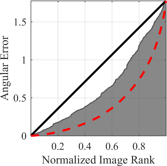
(a) Gehler-Shi dataset [20, 31]

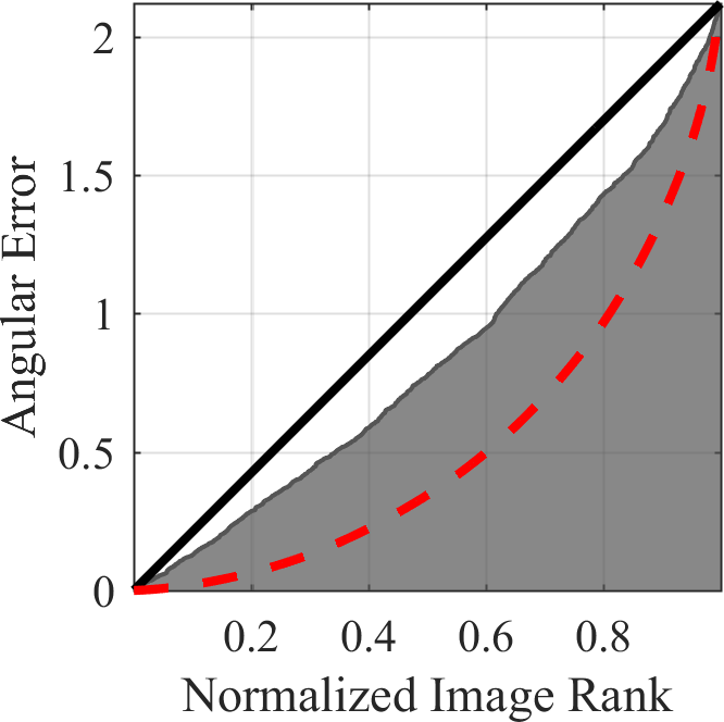
(b) Cheng et al. dataset [12]

EO Error:	1.287	1.696
Mean Error:	1.775	2.121

Figure 6: By sorting each image by the entropy of its posterior distribution we can show that entropy correlates with error. Here we sort the images by ascending entropy and plot the cumulative sum of the error, filling in the area under that curve with gray. If entropy was not correlated with error we would expect the area under the curve to match the black line, and if entropy was perfectly correlated with error then the area under the curve would exactly match the dashed red line. We report twice the area under the curve as “entropy-ordered” error (mean error happens to be twice the area under the diagonal line).

In Figure 22 we visualize a set of images taken from a Nexus 6 in the HDR+ mode [25] after being white-balanced by Model Q in the main paper (the version designed to run on thumbnail images).

Appendix F Color Rendering

All images are rendered by applying the RGB gains implied by the estimated illuminant, applying some color correction matrix (CCM) and then applying an sRGB gamma-correction function (the $C_{\mathrm{linear}}$ to $C_{\mathrm{srgb}}$ mapping in http://en.wikipedia.org/wiki/SRGB). For each camera in the datasets we use we estimate our own CCMs using the imagery, which we present here. These CCMs do not affect our illuminant estimation or our results, and are only relevant to our visualizations. Each CCM is estimated through an iterative least-squares process in which we alternatingly: 1) estimate the ground-truth RGB gains for each image from a camera by solving a least-squares system using our current CCM, and 2) use our current gains to estimate a row-normalized CCM using a constrained least-squares solve. Our estimated ground-truth gains are not used in this paper. For the ground-truth sRGB colors of the Macbeth color chart we use the hex values provided here: http://en.wikipedia.org/wiki/ColorChecker#Colors which we linearize.

$$\small{\mathrm{GehlerShi,Canon1D}}\begin{bmatrix}\phantom{-}2.2310&-1.5926&\phantom{-}0.3616\\ -0.1494&\phantom{-}1.4544&-0.3050\\ \phantom{-}0.1641&-0.6588&\phantom{-}1.4947\\ \end{bmatrix}$$

$$\small{\mathrm{GehlerShi,Canon5D}}\begin{bmatrix}\phantom{-}1.7494&-0.8470&\phantom{-}0.0976\\ -0.1565&\phantom{-}1.4380&-0.2815\\ \phantom{-}0.0786&-0.5070&\phantom{-}1.4284\\ \end{bmatrix}$$

$$\small{\mathrm{Cheng,Canon1DsMkIII}}\begin{bmatrix}\phantom{-}1.7247&-0.7791&\phantom{-}0.0544\\ -0.1436&\phantom{-}1.4632&-0.3195\\ \phantom{-}0.0589&-0.4625&\phantom{-}1.4037\\ \end{bmatrix}$$

$$\small{\mathrm{Cheng,Canon600D}}\begin{bmatrix}\phantom{-}1.8988&-0.9897&\phantom{-}0.0909\\ -0.2058&\phantom{-}1.6396&-0.4338\\ \phantom{-}0.0749&-0.7030&\phantom{-}1.6281\\ \end{bmatrix}$$

$$\small{\mathrm{Cheng,FujifilmXM1}}\begin{bmatrix}\phantom{-}1.4183&-0.2497&-0.1686\\ -0.2230&\phantom{-}1.6449&-0.4219\\ \phantom{-}0.0785&-0.5980&\phantom{-}1.5195\\ \end{bmatrix}$$

$$\small{\mathrm{Cheng,NikonD5200}}\begin{bmatrix}\phantom{-}1.3792&-0.3134&-0.0659\\ -0.0826&\phantom{-}1.3759&-0.2932\\ \phantom{-}0.0483&-0.4553&\phantom{-}1.4070\\ \end{bmatrix}$$

$$\small{\mathrm{Cheng,OlympusEPL6}}\begin{bmatrix}\phantom{-}1.6565&-0.4971&-0.1595\\ -0.3335&\phantom{-}1.7772&-0.4437\\ \phantom{-}0.0895&-0.7023&\phantom{-}1.6128\\ \end{bmatrix}$$

$$\small{\mathrm{Cheng,PanasonicGX1}}\begin{bmatrix}\phantom{-}1.5629&-0.5117&-0.0512\\ -0.2472&\phantom{-}1.7590&-0.5117\\ \phantom{-}0.1395&-0.8945&\phantom{-}1.7550\\ \end{bmatrix}$$

$$\small{\mathrm{Cheng,SamsungNX2000}}\begin{bmatrix}\phantom{-}1.5770&-0.4351&-0.1419\\ -0.1747&\phantom{-}1.5225&-0.3477\\ \phantom{-}0.0573&-0.6397&\phantom{-}1.5825\\ \end{bmatrix}$$

$$\small{\mathrm{Cheng,SonyA57}}\begin{bmatrix}\phantom{-}1.5963&-0.5545&-0.0418\\ -0.1343&\phantom{-}1.5331&-0.3988\\ \phantom{-}0.0563&-0.4026&\phantom{-}1.3463\\ \end{bmatrix}$$

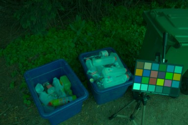
(a) Input Image

(b) Illuminant Posterior

​

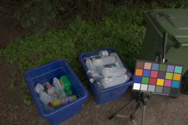
(c) Our prediction

​

(d) Ground Truth

Figure 7: A result from the Gehler-Shi dataset using Model J. Error = $0.02$°, entropy = $-6.48$

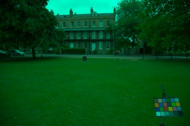
(a) Input Image

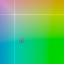
(b) Illuminant Posterior

​

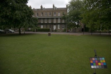
(c) Our prediction

​

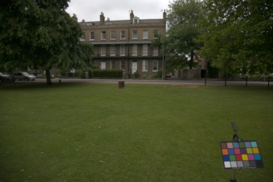
(d) Ground Truth

Figure 8: A result from the Gehler-Shi dataset using Model J. Error = $0.26$°, entropy = $-6.55$

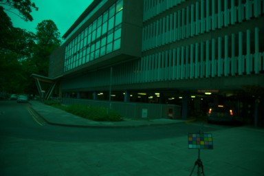
(a) Input Image

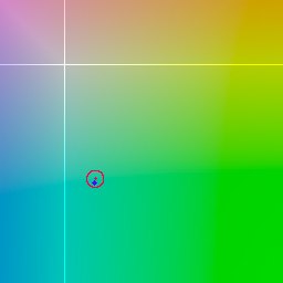
(b) Illuminant Posterior

​

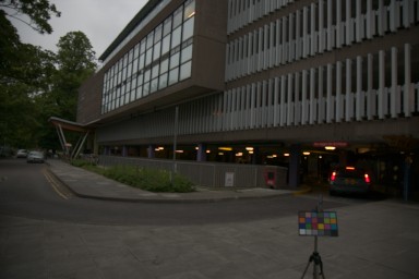
(c) Our prediction

​

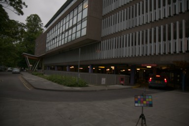
(d) Ground Truth

Figure 9: A result from the Gehler-Shi dataset using Model J. Error = $0.46$°, entropy = $-6.91$

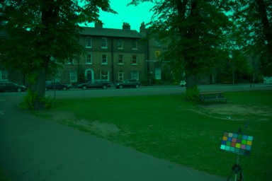
(a) Input Image

(b) Illuminant Posterior

​

(c) Our prediction

​

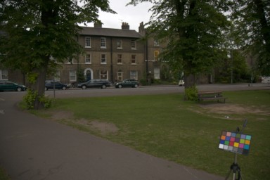
(d) Ground Truth

Figure 10: A result from the Gehler-Shi dataset using Model J. Error = $0.63$°, entropy = $-6.37$

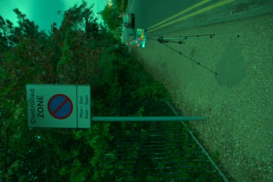
(a) Input Image

(b) Illuminant Posterior

​

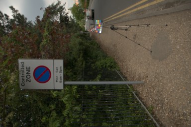
(c) Our prediction

​

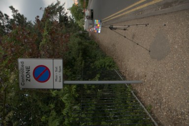
(d) Ground Truth

Figure 11: A result from the Gehler-Shi dataset using Model J. Error = $0.83$°, entropy = $-6.62$

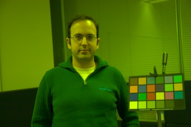
(a) Input Image

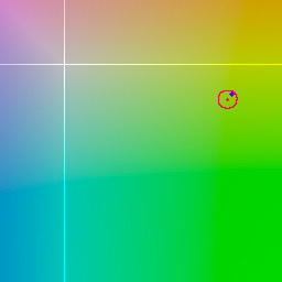
(b) Illuminant Posterior

​

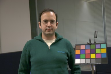
(c) Our prediction

​

(d) Ground Truth

Figure 12: A result from the Gehler-Shi dataset using Model J. Error = $1.19$°, entropy = $-6.71$

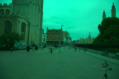
(a) Input Image

(b) Illuminant Posterior

​

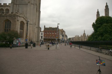
(c) Our prediction

​

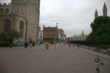
(d) Ground Truth

Figure 13: A result from the Gehler-Shi dataset using Model J. Error = $1.61$°, entropy = $-6.88$

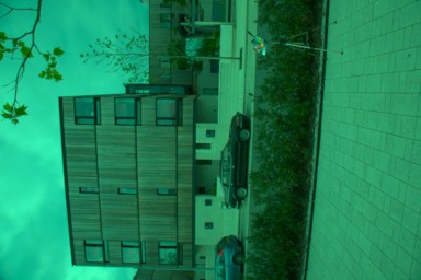
(a) Input Image

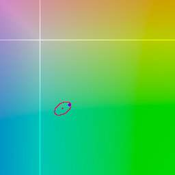
(b) Illuminant Posterior

​

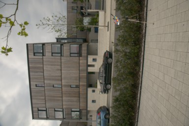
(c) Our prediction

​

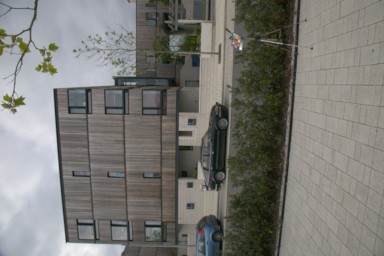
(d) Ground Truth

Figure 14: A result from the Gehler-Shi dataset using Model J. Error = $2.35$°, entropy = $-6.32$

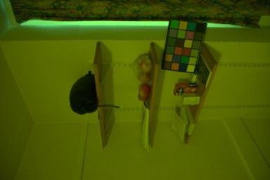
(a) Input Image

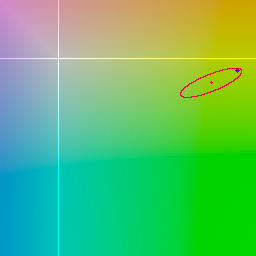
(b) Illuminant Posterior

​

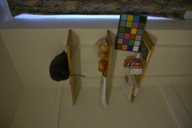
(c) Our prediction

​

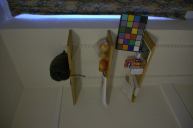
(d) Ground Truth

Figure 15: A result from the Gehler-Shi dataset using Model J. Error = $3.84$°, entropy = $-5.28$

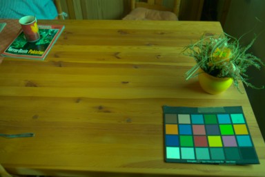
(a) Input Image

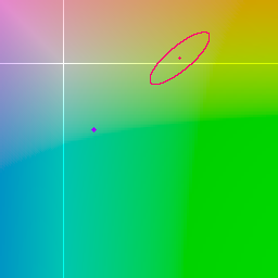
(b) Illuminant Posterior

​

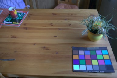
(c) Our prediction

​

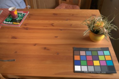
(d) Ground Truth

Figure 16: A result from the Gehler-Shi dataset using Model J. Error = $21.64$°, entropy = $-4.95$

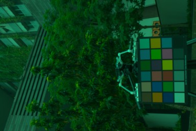
(a) Input Image

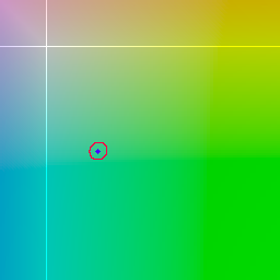
(b) Illuminant Posterior

​

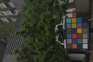
(c) Our prediction

​

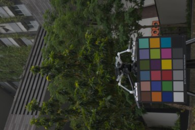
(d) Ground Truth

Figure 17: A result from the Cheng dataset using Model J. Error = $0.12$°, entropy = $-6.82$

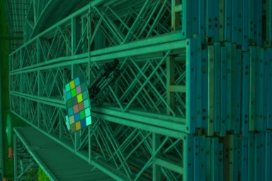
(a) Input Image

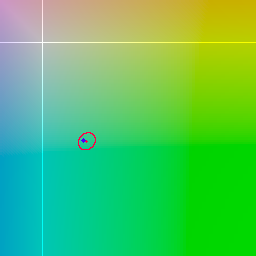
(b) Illuminant Posterior

​

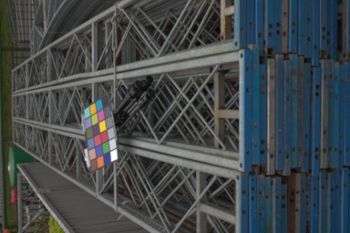
(c) Our prediction

​

(d) Ground Truth

Figure 18: A result from the Cheng dataset using Model J. Error = $0.64$°, entropy = $-6.69$

(a) Input Image

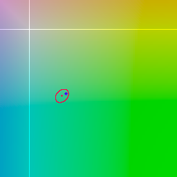
(b) Illuminant Posterior

​

(c) Our prediction

​

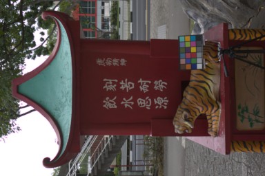
(d) Ground Truth

Figure 19: A result from the Cheng dataset using Model J. Error = $1.37$°, entropy = $-6.48$

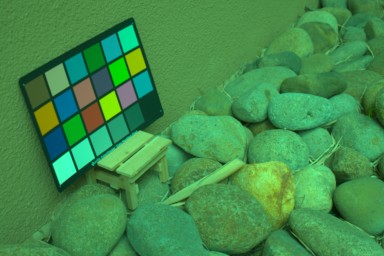
(a) Input Image

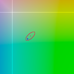
(b) Illuminant Posterior

​

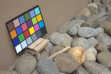
(c) Our prediction

​

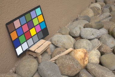
(d) Ground Truth

Figure 20: A result from the Cheng dataset using Model J. Error = $2.69$°, entropy = $-5.82$

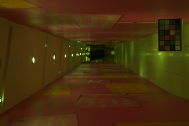
(a) Input Image

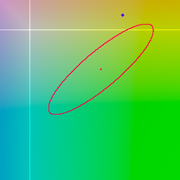
(b) Illuminant Posterior

​

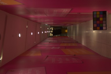
(c) Our prediction

​

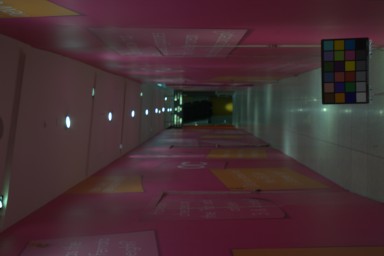
(d) Ground Truth

Figure 21: A result from the Cheng dataset using Model J. Error = $17.85$°, entropy = $-3.04$

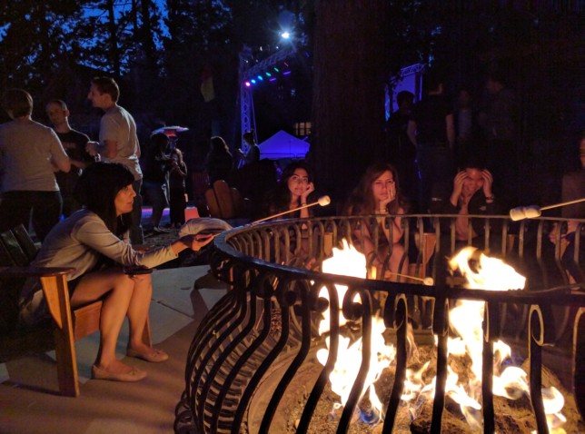
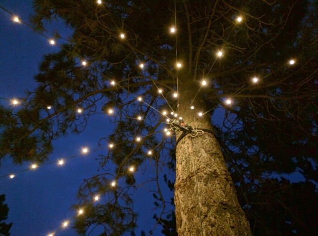
Figure 22: A sampling of unedited HDR+[25] images from a Nexus 6, after being processed with Model Q.

References

- [1] E. H. Adelson and A. P. Pentland. The perception of shading and reflectance. Perception As Bayesian Inference, 1996.
- [2] N. Banic and S. Loncaric. Color dog - guiding the global illumination estimation to better accuracy. VISAPP, 2015.
- [3] K. Barnard, L. Martin, A. Coath, and B. Funt. A comparison of computational color constancy algorithms — part 2: Experiments with image data. TIP, 2002.
- [4] J. T. Barron. Convolutional color constancy. ICCV, 2015.
- [5] H. G. Barrow and J. M. Tenenbaum. Recovering Intrinsic Scene Characteristics from Images. Academic Press, 1978.
- [6] S. Bianco, G. Ciocca, C. Cusano, and R. Schettini. Automatic color constancy algorithm selection and combination. Pattern Recognition, 2010.
- [7] S. Bianco, C. Cusano, and R. Schettini. Color constancy using cnns. CVPR Workshops, 2015.
- [8] D. H. Brainard and B. A. Wandell. Analysis of the retinex theory of color vision. JOSA A, 1986.
- [9] G. Buchsbaum. A spatial processor model for object colour perception. Journal of the Franklin Institute, 1980.
- [10] A. Chakrabarti. Color constancy by learning to predict chromaticity from luminance. NIPS, 2015.
- [11] A. Chakrabarti, K. Hirakawa, and T. Zickler. Color constancy with spatio-spectral statistics. TPAMI, 2012.
- [12] D. Cheng, D. K. Prasad, and M. S. Brown. Illuminant estimation for color constancy: why spatial-domain methods work and the role of the color distribution. JOSA A, 2014.
- [13] D. Cheng, B. Price, S. Cohen, and M. S. Brown. Effective learning-based illuminant estimation using simple features. CVPR, 2015.
- [14] G. D. Finlayson. Corrected-moment illuminant estimation. ICCV, 2013.
- [15] G. D. Finlayson and S. D. Hordley. Color constancy at a pixel. JOSA A, 2001.
- [16] G. D. Finlayson and E. Trezzi. Shades of gray and colour constancy. Color Imaging Conference, 2004.
- [17] D. H. Foster. Color constancy. Vision research, 2011.
- [18] B. V. Funt and W. Xiong. Estimating illumination chromaticity via support vector regression. Color Imaging Conference, 2004.
- [19] S. Gao, W. Han, K. Yang, C. Li, and Y. Li. Efficient color constancy with local surface reflectance statistics. ECCV, 2014.
- [20] P. Gehler, C. Rother, A. Blake, T. Minka, and T. Sharp. Bayesian color constancy revisited. CVPR, 2008.
- [21] A. Gijsenij and T. Gevers. Color constancy using natural image statistics and scene semantics. TPAMI, 2011.
- [22] A. Gijsenij, T. Gevers, and J. van de Weijer. Generalized gamut mapping using image derivative structures for color constancy. IJCV, 2010.
- [23] A. Gijsenij, T. Gevers, and J. van de Weijer. Computational color constancy: Survey and experiments. TIP, 2011.
- [24] T. Hamelryck, K. Mardia, and J. Ferkinghoff-Borg. Bayesian methods in structural bioinformatics. Springer, 2012.
- [25] S. W. Hasinoff, D. Sharlet, R. Geiss, A. Adams, J. T. Barron, F. Kainz, J. Chen, and M. Levoy. Burst photography for high dynamic range and low-light imaging on mobile cameras. SIGGRAPH Asia, 2016.
- [26] H. R. V. Joze and M. S. Drew. Exemplar-based color constancy and multiple illumination. TPAMI, 2014.
- [27] E. H. Land and J. J. McCann. Lightness and retinex theory. JOSA, 1971.
- [28] K. V. Mardia. Statistics of directional data. Journal of the Royal Statistical Society, Series B, 1975.
- [29] J. Ragan-Kelley, A. Adams, S. Paris, M. Levoy, S. Amarasinghe, and F. Durand. Decoupling algorithms from schedules for easy optimization of image processing pipelines. SIGGRAPH, 2012.
- [30] L. I. Rudin, S. Osher, and E. Fatemi. Nonlinear total variation based noise removal algorithms. Physica D: Nonlinear Phenomena, 1992.
- [31] L. Shi and B. Funt. Re-processed version of the gehler color constancy dataset of 568 images. http://www.cs.sfu.ca/ colour/data/.
- [32] W. Shi, C. C. Loy, and X. Tang. Deep specialized network for illuminant estimation. ECCV, 2016.
- [33] J. van de Weijer, T. Gevers, and A. Gijsenij. Edge-based color constancy. TIP, 2007.
- [34] J. van de Weijer, C. Schmid, and J. Verbeek. Using high-level visual information for color constancy. ICCV, 2007.
- [35] J. Wang, Y. Song, T. Leung, C. Rosenberg, J. Wang, J. Philbin, B. Chen, and Y. Wu. Learning fine-grained image similarity with deep ranking. CVPR, 2014.
- [36] K.-F. Yang, S.-B. Gao, and Y.-J. Li. Efficient illuminant estimation for color constancy using grey pixels. CVPR, 2015.