if RespIllness and Smoker and Age>=50: LungCancer
elif RiskDepression: Depression
elif BMI>=0.2 and Age>=60: Diabetes
elif Headaches and Dizziness: Depression
elif DocVisits>=0.3: Diabetes
elif DispTiredness: Depression
else: Diabetes\end{lstlisting}
%}
\caption{Decision list}
\label{fig:declist}
\end{subfigure}
\\
%\quad
\begin{subfigure}{0.9\textwidth}
\begin{lstlisting}[language=Python]
if RespIllness and Smoker and Age>=50: LungCancer
if RiskLungCancer and BP>=0.3: LungCancer
if RiskDepression and PastDepression: Depression
if BMI>=0.3 and Insurance=None and BP>=0.2: Depression
if Smoker and BMI>=0.2 and Age>=60: Diabetes
if RiskDiabetes and BMI>=0.4 and ProbInfections>=0.2: Diabetes
if DocVisits>=0.4 and ChildObesity: Diabetes\end{lstlisting}
\caption{Decision Set}
\label{fig:decset}
\end{subfigure}
\caption{Example of programs for a decision set and a decision list, originally appearing in ~\citet{lakkaraju16:interpretable}, demonstrating that they remain easy to read as programs. These were written manually.}
\label{fig:decs}
\end{figure}
\section{Other Interpretable Representations as Programs}
\label{sec:prog}
In this section we provide some simple examples of interpretable models currently used in the literature, and describe how their programmatic equivalent would look like.
As it will become apparent, most of these existing interpretable models retain their readability when written as programs.
We use a fairly simple but expressive language for our programs that consists of boolean constants (\texttt{True}, \texttt{False}) and operators (\texttt{and}, \texttt{or}, \texttt{not}), absence/presence of the features of the input instance (\texttt{Smoker}), real valued constants (\texttt{0.5}) and algebraic operators (\texttt{+,-,*}), real-valued features (\texttt{Age}), and if-then-else conditions.
This language is fairly expressive, but due to the lack of looping, recursion, and variables, is still not a complete programming language.
We will use the Python syntax to render our programs, slightly abused to conserve space.
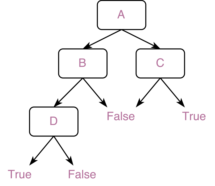
One of the most commonly used interpretable representations is that of decision trees~\cite{craven96:extracting}.
From the simple decision tree in Figure~\ref{fig:dectree}, along with the program for it in Figure~\ref{fig:dectree:prog}, it is clear that the program is a fairly intuitive representation.
Along with decision trees, sparse linear models have also been used in a number of applications as interpretable representations of machine learning~\cite{ustun15:supersparse}.
In Figure~\ref{fig:linprog}, we shows two programs: first that exactly captures the behavior over the relevant features, while the second demonstrates a simpler program that has the same behavior if the features are binary and the prediction is true if the linear model evaluates to a positive score.
Recently, decision lists~\cite{wang15:falling,letham15:interpretable} and decision sets~\cite{lakkaraju16:interpretable} have been introduced as more comprehensible representations than decision trees, while being much more powerful that linear models.
Since these are often presented using pseudo code, the program for these representations in our language looks essentially the same, as shown in Figure~\ref{fig:decs}.
%\cite{caruana15:intelligible}
From these examples, it is clear that not only are programs able to represent the different interpretable representations succinctly, but the programming language can be much more expressive than any single representation.
The key challenges is to actually synthesize the appropriate program, i.e. to make sure it is both a good approximation of the black-box model, and is as readable as the examples shown here.
In the next section we will formalize this problem, and describe a prototype solution.
\section{Inducing Program Explanations}
\label{sec:inducing}
In this section, we briefly outline our ideas on how to generate programs as explanations for complex systems, along with the description of a prototype implementation using simulated annealing.
\textbf{Local, Model-Agnostic Explanations:}
Our goal here is to explain individual predictions of a complex machine learning system, by treating them in a black-box manner.
The advantages of generating such model-agnostic explanations was described in \citet{ribeiro16:model-agnostic}.
Our proposed work builds upon the ideas in \citet{ribeiro16:kdd}.
Let the black-box system be $f:\mathcal{X}\rightarrow\{0,1\}$, and we are interested in explaining a specific prediction, i.e. $f(x)=y$.
In order to generate an explanation that describes the behavior of $f$ around $x$, we generate a number of random perturbations of $x$, denoted by $Z$.
We then induce the program that both (1) accurately models the behavior of $f$ on the samples $Z$ (weighed by their similarity to $x$), and (2) is interpretable to the user.
Specifically, we solve the following optimization:
\begin{equation}
\hat{p} = \underset{p\in\mathcal{P}}{\arg\min}~\mathcal{L}(f, p, Z, \Pi_x) + \Omega(p)\label{eq:opt}
\end{equation}
where $P$ is the set of compatible programs (valid expressions that $\mathcal{X}\rightarrow\{0,1\}$), $\mathcal{L}(f,p,Z,\Pi_x)$ is the loss between the outputs of $f$ and $p$ on the samples $Z$ weighted by $\Pi_x$, and $\Omega(\cdot)$ denotes the complexity of the program (number of lines or the depth of the expression tree, for example).
\textbf{Program Induction:}
Eq~\eqref{eq:opt} is a challenging combinatorial optimization on a potentially complex surface (depending on the loss used).
A related thread of research is \emph{program induction}, where programs are synthesized automatically to match some desired goal~\cite{manna80:a-deductive}.
Number of different variations of this problem have been introduced, depending on the syntax of the program and the formalism of the desired goals, with solvers ranging from genetic programming~\cite{briggs06:functional} to MCMC~\cite{liang10:learning}.
There has also been recent work in using probabilistic programs to identify such programs, mentioned as a possibility in \citet{mansinghka09:natively} using Church~\citep{goodman08:church:}, but with a recent implementation by \citet{gaunt16:terpret:}.
However, we were unable to identify an off-the-shelf program inducer that can support an arbitrary loss (that depends on the domain) in order to identify the appropriate explanation.
\textbf{Prototype Implementation:}
We implemented a prototype program inducer that approximately solves Eq~\eqref{eq:opt} in order to generate program explanations.
We use the same syntax as the one used in Section~\ref{sec:prog}, i.e. boolean constants and operators, input features, real-valued constants and algebraic operators, and if-then-else conditions.
In order to encapsulate the complexity of each program, we set $\Omega(.)$ to be $0$ if the number of nodes in the expression tree is $<$8 and is $\infty$ otherwise, i.e. we are implicitly considering a family of short programs as $\mathcal{P}$.
We use the negative of the weighted $F_1$ score as the loss $\mathcal{L}$, but the implementation supports any arbitrary function that is evaluated on the outputs of $f$ and $p$ on $Z$.
The combinatorial optimization is solved using simulated annealing~\cite{kirkpatrick83:optimization} with a logarithmically decreasing temperature schedule, and a proposal function that randomly grows, shrinks, or replaces nodes in the express tree to create valid perturbed expression trees.
\section{Example Generated Programs}
Using the program induction technique described in the previous section, here we present a few example program explanations for a number of classifiers (treated as black-boxes) on two datasets from the UCI repository~\cite{lichman13:uci-machine}: \emph{adult} and \emph{hospital readmission}.
In order to evaluate whether the programs are accurate as explanations, we also provide a visualization of the decision tree models.
In Figures \ref{fig:adult:tree} and \ref{fig:readmiss:tree} we show the learned decision tree on these datasets.
We also trained a random forest classifier and a logistic regression model.
Figures \ref{fig:adult:expl} and \ref{fig:readmiss:expl} show the generated program explanations for both the datasets, demonstrating that the programs are compact and readable, and ones for the decision trees are accurate to the model as well.
Further, it is clear that random forests, which is much more complex in structure than trees or linear models, requires more complicated programs as explanations, however these programs still make sense (Figure \ref{fig:adult:expl}, in particular).
\begin{figure}[tb]
\begin{subfigure}{0.55\textwidth}
\includegraphics[width=\textwidth]{adult-tree}
\caption{Decision tree (with the path highlighted)}
\label{fig:adult:tree}
\end{subfigure}
\quad
% \begin{subfigure}{0.3\textwidth}
% \includegraphics[width=\textwidth]{figs/dec-tree}
% \caption{Linear model}
% \label{}
% \end{subfigure}
%\quad
\begin{subfigure}{0.4\textwidth}
\textbf{Random Forests} (true implies $>50$K):
\begin{lstlisting}[language=Python]
(if HoursPerWeek<=40:
CapitalGain>0
else: True) and Married\end{lstlisting}
\textbf{Decision Tree} (true implies $>50$K):
\begin{lstlisting}[language=Python]
CapitalGain>0 and Married\end{lstlisting}
\textbf{Linear model} (true implies $>50$K):
\begin{lstlisting}[language=Python]
if CapitalGain>0: Married
else : False\end{lstlisting}
\caption{Generated program explanations}
\label{fig:adult:expl}
\end{subfigure}
\caption{\textbf{Adult dataset:} In (a), we show the learned tree, with the path for the instance in blue, and in red, we show that \texttt{Education} doesn’t really matter for this instance. (b) shows the explanations for three classifiers (they got the prediction right), in particular showing that the explanation for the decision tree gets the more compact form.}
\label{fig:adult}
\end{figure}
\begin{figure}[tb]
\begin{subfigure}{0.4\textwidth}
\includegraphics[width=\textwidth]{readmiss-tree}
\caption{Decision tree (with the path highlighted)}
\label{fig:readmiss:tree}
\end{subfigure}
\qquad
% \begin{subfigure}{0.3\textwidth}
% \includegraphics[width=\textwidth]{figs/dec-tree}
% \caption{Linear model}
% \label{}
% \end{subfigure}
%\quad
\begin{subfigure}{0.5\textwidth}
\textbf{Random Forests} (true implies $<30$):
\begin{lstlisting}[language=Python]
if Diag:Other and not Tolbutamide:
Discharged:Home
else: Diag:Other\end{lstlisting}
\textbf{Decision Tree} (true implies $>30$):
\begin{lstlisting}[language=Python]
NumInpatient > 1.00\end{lstlisting}
\textbf{Linear model} (true implies NO):
\begin{lstlisting}[language=Python]
not Tolazamide\end{lstlisting}
\caption{Generated program explanations}
\label{fig:readmiss:expl}
\end{subfigure}
\caption{\textbf{Hospital Readmission data:} (a) shows the learned tree, with the path for the instance in blue. Again, (b) shows the explanations for three classifiers (only the tree had the correct prediction), with the compact explanation for tree almost correct, except that it assumes the patient is alive.}
\label{fig:readmiss}
\end{figure}
\section{Conclusions and Future Work}
In this paper we motivated the need to use programs as model-agnostic explanations: programs are designed to be intuitive to humans and are incredibly expressive.
We presented a prototype implementation that induces programs as local explanations of a classifier by fitting to the classifier’s predictions on a set of perturbations of the instance being explained.
We demonstrated example explanations generated for multiple datasets and classifiers.
There are a number of exciting avenues for future work on these ideas.
We will investigate methods for inducing programs with a much more expressive syntax, including, for example, loops and variables.
Instead of relying on combinatorial optimization techniques that may not scale to applications on more complex domains, syntax, and systems, we will explore the use of recently introduced \emph{differentiable} program induction techniques such as in \citet{neelakantan2015neural} and \citet{riedel16:programming}.
%We are also interested in exploring different \emph{objectives} when inducing programs since different applications may want to focus on different evaluation
% - induce probabilistic programs
%- experiment with different \emph{objectives}, focus on precision, etc.
Finally, on real-world applications and using user studies, we will thoroughly evaluate the interpretability and utility of using programs as local explanations of complex machine learning systems.
%- deploy on complex decision pipelines, not just machine learning classifiers.
%- human experiments
% \subsubsection*{Acknowledgments}
%
% Use unnumbered third level headings for the acknowledgments. All
% acknowledgments go at the end of the paper. Do not include
% acknowledgments in the anonymized submission, only in the final paper.
% vision: karpathy15:deep,kim15:ibcm:, bansal14:towards, goyal16:interpreting, \cite{xu15:show}
% HCI: amershi15:modeltracker:, krause16:interacting, patel10:gestalt:,
%\cite{kulesza15:principles}\cite{dzindolet03:the-role}
%\newpage
\small
\bibliographystyle{plainnat}
% \bibliographystyle{abbrvnat}
% \setcitestyle{year}
\bibliography{../sameer}
\end{document}