Geometrical Clusterization in SU(2) gluodynamics and Liquid-gas Phase Transition

Abstract

The liquid droplet formula is applied to an analysis of the properties of geometrical (anti)clusters formed in SU(2) gluodynamics by the Polyakov loops of the same sign. Using this approach, we explain the phase transition in SU(2) gluodynamics as a transition between two liquids during which one of the liquid droplets (the largest cluster of a certain Polyakov loop sign) experiences a condensation, while another droplet (the next to the largest cluster of the opposite sign of Polyakov loop) evaporates. The clusters of smaller sizes form two accompanying gases, which behave oppositely to their liquids. The liquid droplet formula is used to analyze the size distributions of the gas (anti)clusters. The fit of these distributions allows us to extract the temperature dependence of surface tension and the value of Fisher topological exponent $\tau$ for both kinds of gaseous clusters. It is shown that the surface tension coefficient of gaseous (anti)clusters can serve as an order parameter of the deconfinement phase transition in SU(2) gluodynamics. The Fisher topological exponent $\tau$ of (anti)clusters is found to have the same value $1.806\pm 0.008$. This value disagrees with the famous Fisher droplet model, but it agrees well with an exactly solvable model of nuclear liquid-gas phase transition. This finding may evidence for the fact that the SU(2) gluodynamics and this exactly solvable model of nuclear liquid-gas phase transition are in the same universality class.

Kewords: geometrical clusters, size distributions, liquid droplet model formula, surface tension

Bogolyubov Institute for Theoretical Physics, Kyiv, Ukraine.

FIAS, Frankfurt upon Main, Germany.

Introduction

The lattice formulation of quantum chromodynamics (QCD) is presently considered as the only first principle tool to investigate a transition between the confined and deconfined states of strongly interacting matter. Such a phase transition (PT) is also expected in a pure non abelian SU(N) gauge theory which is known as gluodynamics. The Svetitsky-Jaffe hypothesis [Yaffe and Svetitsky, 1982] relates the deconfinement PT in (d+1)-dimensional SU(N) gluodynamics to the magnetic PT in the d-dimensional Z(N) symmetric spin model. The key element of this correspondence is that the role of spin in the original SU(N) gluodynamics is played by the so called Polyakov loop. The latter is interpreted as the time propagator of an infinitely heavy static quark. A high level of understanding of the spin systems along with the Svetitsky-Jaffe hypothesis led to a significant progress in studies of the SU(N) gluodynamics properties in the PT vicinity. Formation of geometrical clusters composed of the Polyakov loops is an important feature of the pure gauge theories [Fortunato and Satz, 2000, Fortunato et al., 2001]. A similar phenomenon is well known in spin systems and it is responsible for percolation of clusters. Moreover, the deconfinement PT in gluodynamics already was studied within the percolation framework in Refs. [Gattringer, 2010, Gattringer and Schmidt, 2011], where the main attention was paid to the largest and the next to the largest clusters whereas the smaller clusters were ignored. However, in many respects the PT details are encoded in the properties of smaller clusters which is well-known after formulating the Fisher Droplet Model (FDM) [Fisher, 1967,1969]. An important finding of the FDM is that at the critical point the size distribution of physical clusters obeys a power law which is controlled by the Fisher topological exponent $\tau$. Hence the value of this exponent is rather important in order to develop a consistent theory of PT in strongly interacting matter and to localize the critical point of QCD phase diagram which is a hot topic of the physics of heavy ion collisions. Therefore, in this work we study the geometrical clusterization in SU(2) gluodynamics and analyze the properties of clusters of all possible sizes. Such an approach allows us to explain the deconfinement of color charges as a specific kind of the liquid-gas PT [Ivanytskyi et al., 2016].

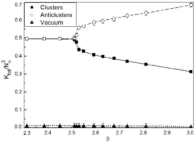
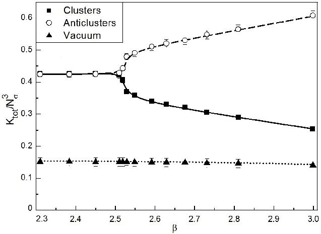
Figure 1.: Total volume fraction of clusters, anticlusters and auxiliary vacuum measured for $L_{cut}=0.1$ (left panel) and $L_{cut}=0.2$ (right panel). The volume fraction of an auxiliary vacuum is independent on the Polyakov loop cut off. The curves are shown to guide the eye.

The Polyakov loop geometrical clusters

The local Polyakov loop is a gauge invariant analog of continuous spin which exists in every space point of the lattice. In case of discrete (d+1)-dimensional lattice of size $N_{\sigma}^{d}\times N_{\tau}$ it is defined by the trace of temporal gauge links $U_{4}(\vec{x},t)$

$$L(\vec{x})=Tr\prod_{t=0}^{N_{\tau}-1}U_{4}(\vec{x},t).$$ (1)

In case of $SU(2)$ gauge group the quantity $L(\vec{x})$ has real values in the interval from $-1$ to $1$. For a given lattice configuration the neighboring Polyakov loops can be attributed to one cluster, if they have the same sign. The boundaries of clusters with opposite signs of Polyakov loop are characterized by the strong fluctuations of $L(\vec{x})$. Therefore, similarly to Refs. [Gattringer, 2010, Gattringer and Schmidt, 2011] we introduced the minimal absolute value of the Polyakov loop attributed to the clusters, i.e. a cut off parameter $L_{cut}>0$. All space points $\vec{x}$ with $|L(\vec{x})|\leq L_{cut}$ are attributed to “auxiliary” or “confining” vacuum which volume fraction is independent of the inverse lattice coupling $\beta=\frac{4}{g^{2}}$ (see Fig. 1), where $g^{2}$ is the lattice coupling constant. The above definition allows us to define the monomers, the dimers, etc. as the clusters made of a corresponding number of “gauge spins” of the same sing which are surrounded either by the clusters of the opposite “spin” sign or by a vacuum [Ivanytskyi et al., 2016]. Obviously, there are clusters of two types related to two signs of the local Polyakov loop. We introduce a formal definition of anticlusters, if their sign coincides with the sign of the largest n-mer existing at a given lattice configuration. The largest anticluster is called the “anticluster droplet” whereas the other n-mers of the same sign correspond to the “gas of anticlusters”. The clusters are defined to have an opposite sign of the Polyakov loop, whereas the largest of them is called the “cluster droplet”.

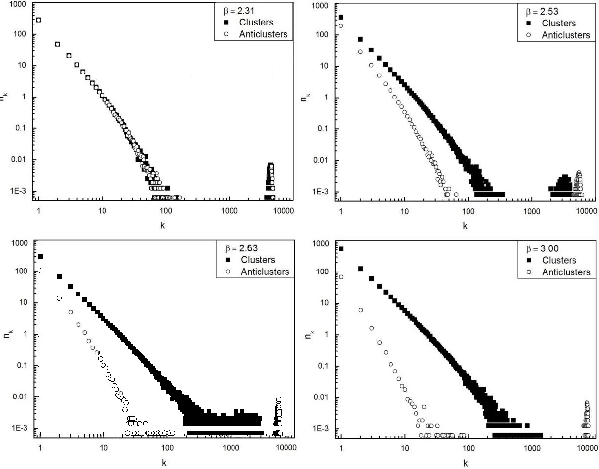
Figure 2.: Size distributions of clusters (squares) and anticlusters (circles) for $\beta=2.31$ (left upper panel), $\beta=2.53$ (right upper panel), $\beta=3.0$ (lower panel) are shown for the cut off $L_{cut}=0.2$.

Size distributions of clusters

The described scheme of the (anti)cluster identification was realized numerically. The Polyakov loops were obtained at each spatial point of 3+1 dimensional lattice with the spatial and temporal extents $N_{\sigma}=24$ and $N_{\tau}=8$, respectively. The simulations were performed for 13 values of the inverse lattice coupling $\beta$ inside the interval $\beta\in[2.31,3]$. The physical temperature $T$ is unambiguously defined by the temporal extent and the lattice spacing $a$ as $1/T=N_{\tau}a$. The $\beta$ points where distributed not uniformly. They where concentrated in the PT region which is of principal interest for this study. The identification of (anti) clusters was performed for two values of the Polyakov loop cut off $L_{cut}=0.1$ and $0.2$. For almost all $\beta$ points the number of (anti)clusters of each size was averaged over the ensemble of 800 and 1600 gauge field lattice configurations. The distributions obtained in this way were practically the same (within the statistical errors). Hence, in our analysis we used the results found for 1600 configurations as the high statistics limit. In case of gaseous anticlusters at three largest values of $\beta$ the statistics was rather poor. Therefore, for these points we used 2400 configurations. The right hand side vicinity of PT was also analyzed with higher statistics in order to exclude the effects of statistical fluctuations which we observed for $\beta=2.52,~{}2.53$ and $2.67$. The typical size distributions of (anti)clusters $n_{k}$ for $L_{cut}=0.2$ are shown in Fig. 2. For the lattice constant values below the critical value $\beta_{c}^{\infty}=2.5115$ in an infinite system [Fingberg et al., 1993] the distributions of (anti)clusters are identical due to existing global Z(2) symmetry (the left upper panel of Fig. 2). If $\beta$ is even slightly above $\beta_{c}^{\infty}$ then the symmetry between (anti)clusters breaks down (the right upper panel of Fig. 2). In this case the size of the cluster (anticluster) droplet decreases (increases). It is remarkable, that the corresponding gaseous clusters behave contrary to their droplets. Therefore, the deconfinement PT in SU(2) gluodynamics can be considered as an evaporation of the cluster droplet into the gas of clusters and a simultaneous condensation of the gas of anticlusters into the anticluster droplet. At high $\beta$ (the lower panel of Fig. 2) the cluster droplet becomes indistinguishable from its gas whereas the size of anticluster droplet becomes comparable to the size of system. From Fig. 2 one can see that the gas and liquid branches of anticluster distributions are well separated from each other. A similar behavior is seen for the clusters, except for very high values of $\beta$, where the cluster droplet simply disappears due to evaporation (see the lower panel of Fig. 2).

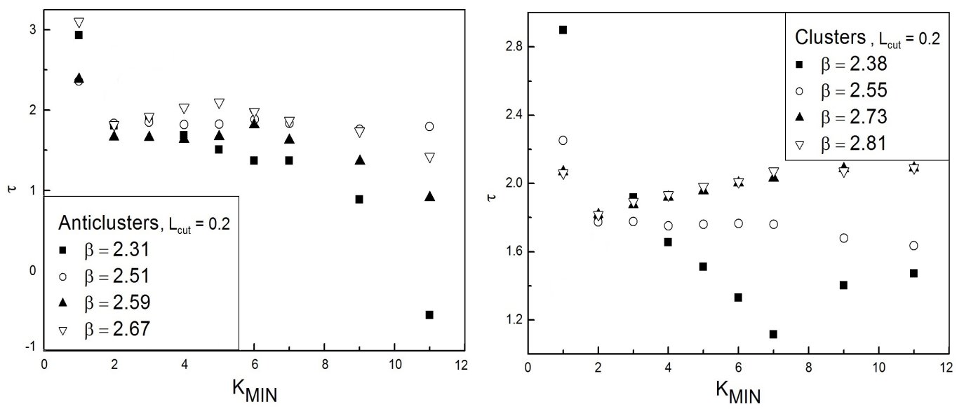
Figure 3.: The Fisher exponent $\tau$ for several values of $k_{min}$ and for a few values of $\beta$ found by the 4-parametric fit of the LDM formula. All these results refer to the cut-off $L_{cut}=0.2$.

Since the found distributions closely resemble the ones discussed for the nuclear fragments and for the Ising spin clusters [Sagun et al., 2014], we decided to study the question whether the Liquid Droplet Formula (LDF) [Fisher, 1967]

$$n_{A}^{th}(k)=C_{A}\exp\left(\mu_{A}k-\sigma_{A}k^{2/3}-\tau\ln k\right)\,,$$ (2)

is able to reproduce the size distributions of clusters ($A=cl$) and anticlusters ($A=acl$). Here $\mu_{A}k$ is the bulk part of free energy of k-mer (anti)cluster, $\sigma_{A}k^{2/3}$ denotes its surface free energy with the surface proportional to $k^{2/3}$, $\tau$ is the Fisher topological constant and $C_{A}$ is the normalization factor. These parameters were defined from the fit of the (anti)cluster size distributions. Since the LDM is valid only for (anti)clusters which are sufficiently large, then the question which has to be clarified first was a determination of the minimal size $k_{min}$ to which Eq. (2) can be applied. A minimization of the quantity

$$\frac{\chi^{2}}{dof}=\frac{1}{k_{max}-k_{min}-4}\sum_{k=k_{min}}^{k_{max}}\left(\frac{n_{A}^{th}(k)-n_{A}(k)}{\delta n_{A}(k)}\right)^{2}\,,$$ (3)

with respect to $C_{A}$, $\mu_{A}$, $\sigma_{A}$, $\tau$ and $k_{min}$ allowed us to answer this question. Here $k_{max}$ is the maximal size of the gaseous (anti)cluster and $\delta n_{A}(k)$ denotes the error of $n_{A}(k)$ obtained in simulations. In practice, the minimization procedure was performed using the iterative gradient search method, in which the next approximation of the parameter vector $\vec{p}_{A}=(C,\mu,\sigma,\tau)_{A}$ is defined as

$$\vec{p}_{A}\rightarrow\vec{p}_{A}-\epsilon\cdot\vec{\nabla}_{\vec{p}_{A}}\frac{\chi^{2}}{dof}\;,$$ (4)

while the positive valued elements of the matrix $\epsilon=diag(\epsilon_{C},\epsilon_{\mu},\epsilon_{\sigma},\epsilon_{\tau})$ are used in order to optimize the fit procedure. Evidently, this iterative scheme corresponds to a numerical solution of the equation $\vec{\nabla}_{\vec{p}_{A}}\frac{\chi^{2}}{dof}=0$ which is a criterion of $\frac{\chi^{2}}{dof}$ minimization. A comparison of the fit quality obtained for different $k_{min}$ values shows that the LDF is already able to describe the dimers. Indeed, we found that $\frac{\chi^{2}}{dof}\approx 1$ for all $k_{min}\geq 2$ , whereas for $k_{min}=1$ we got $\frac{\chi^{2}}{dof}\approx 10$ which corresponds to the low quality of data description. Our analysis of the Fisher topological constant behavior as a function of $\beta$ demonstrates that for $k_{min}=2$ it is, indeed, a constant within the statistical errors (see Fig. 3). This remarkable result is in line with predictions of the cluster type models [Fisher, 1967,1969, Sagun et al., 2014]. Moreover, we found that $\tau<2$ both for clusters and for anticlusters. This result agrees with the exactly solvable model of the nuclear liquid-gas phase transition [Sagun et al., 2014] and contradicts to the FDM [Fisher, 1967,1969]. Thus, performing a four parametric fit of the LDF we found that $k_{min}=2$ and $\tau=1.806\pm 0.008$ both for clusters and for anticlusters. After fixing the value of $\tau$ exponent, we used a three parametric fit of the (anti)cluster size distributions to define $C_{A}$, $\mu_{A}$ and $\sigma_{A}$ with high precision. This was done by minimizing $\frac{\chi^{2}}{dof}$ for $k_{min}=2$ and $\tau=1.806$. The typical value of $\frac{\chi^{2}}{dof}\approx 1$ was obtained for any $\beta$, which signals about the high quality of the data description. The $\beta$-dependences of $\mu_{A}$ and $\sigma_{A}$ are shown in Fig. 4 for $L_{cut}=0.2$. For $L_{cut}=0.1$ the results are qualitatively the same.

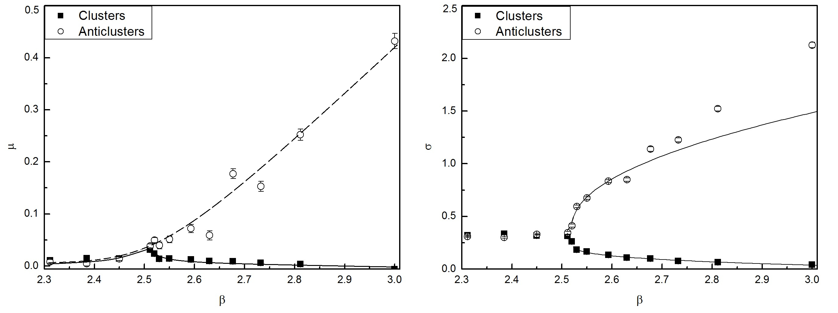
Figure 4.: Dependence of the reduced chemical potential $\mu_{A}$ (left panel) and the reduced surface tension $\sigma_{A}$ (right panel) on the inverse lattice coupling $\beta$ obtained for $L_{cut}=0.2$. The curves shown in the right panel represent Eq. (5).

Order parameters of the deconfinement phase transition

From the right panel of Fig. 4 one can see that the behavior of the reduced surface tension coefficient $\sigma_{A}$ drastically changes when $\beta$ exceeds the critical value $\beta_{c}=2.52$. Indeed, for $\beta\leq\beta_{c}$ this quantity is constant and it is identical for clusters and anticlusters, while for $\beta>\beta_{c}$ the situation is completely different, since $\sigma_{cl}$ monotonically decreases and $\sigma_{acl}$ monotonically increases with $\beta$. The qualitatively different behavior of these quantities allows us to treat them as an order parameter of the deconfinement PT in SU(2) gluodynamics. The $\beta$-dependence of the reduced surface tension in the right hand side vicinity of $\beta_{c}$ can be successfully described by the exponent $B_{A}$ as

$$\sigma_{A}(\beta)=\sigma_{A}(\beta_{c})\pm d_{A}(\beta-\beta_{c})^{B_{A}},$$ (5)

where the signs “+” and “-” correspond to A=acl and A=cl, respectively, and $d_{A}$ is the normalization constant. The $\beta$-dependence of $\sigma_{A}$ was described by this formula. The results of fit are given in Table 1. Despite the different values of $d_{A}$ found for different cut offs, the exponents $B_{A}$ do not show any dependence on $L_{cut}$.

Table 1.: The fit parameters according to Eq. (5).

cut-off	type	$d_{A}$	$B_{A}$	$\chi^{2}/dof$
$L_{cut}=0.1$	clusters	$0.485\pm 0.014$	$0.2920\pm 0.0012$	$1.43/4\simeq 0.36$
$L_{cut}=0.1$	anticlusters	$2.059\pm 0.028$	$0.4129\pm 0.0077$	$1.68/4\simeq 0.48$
$L_{cut}=0.2$	clusters	$0.2796\pm 0.0118$	$0.2891\pm 0.0016$	$1.11/4\simeq 0.28$
$L_{cut}=0.2$	anticlusters	$1.344\pm 0.033$	$0.4483\pm 0.0021$	$0.66/2\simeq 0.33$

The mean size of the droplet we found according to the expression

$$\max K_{A}=\frac{\sum\limits_{k=1}k^{1+\tau}n_{A}(k)}{\sum\limits_{k=1}k^{\tau}n_{A}(k)}\,.$$ (6)

The $\beta$-dependence of $\max K_{A}$ is shown in Fig. 5. Its behavior for $\beta>\beta_{c}$ is described by the exponent $b_{A}$

$$\max K_{A}(\beta)=\max K_{A}(\beta_{c})\pm a_{A}(\beta-\beta_{c})^{b_{A}},$$ (7)

where the signs “+” and “-” correspond to A=acl and A=cl, respectively, and $a_{A}$ is the normalization constant. The parameters found by the fit are given in Table 2.

Table 2.: The fit parameters according to Eq. (7).

cut-off	type	$a_{A}$	$b_{A}$	$\chi^{2}/dof$
$L_{cut}=0.1$	clusters	$3056\pm 246$	$0.2964\pm 0.0284$	$16.32/4\simeq 4.08$
$L_{cut}=0.1$	anticlusters	$2129\pm 160$	$0.3315\pm 0.0269$	$8.94/4\simeq 2.235$
$L_{cut}=0.2$	clusters	$4953\pm 443$	$0.3359\pm 0.0289$	$12.3/3\simeq 4.01$
$L_{cut}=0.2$	anticlusters	$2462\pm 87.7$	$0.3750\pm 0.0129$	$2.068/4\simeq 0.517$

It is remarkable that the found exponents $b_{A}$ are close to the critical exponent $\beta_{Ising}=0.3265\pm 0.0001$ of the 3-dimensional Ising model [Campostrini et al., 2002] and to the critical exponent $\beta_{liquids}=0.335\pm 0.015$ of simple liquids [Huang, 1987], whereas for $L_{cut}=0.2$ the exponent $b_{acl}$ is somewhat larger.

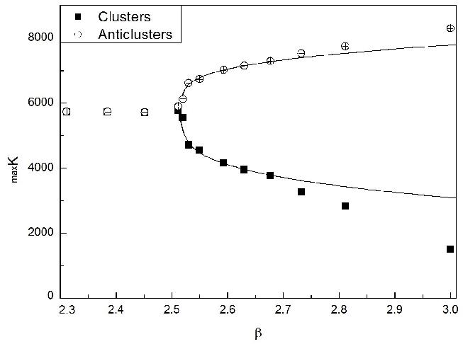
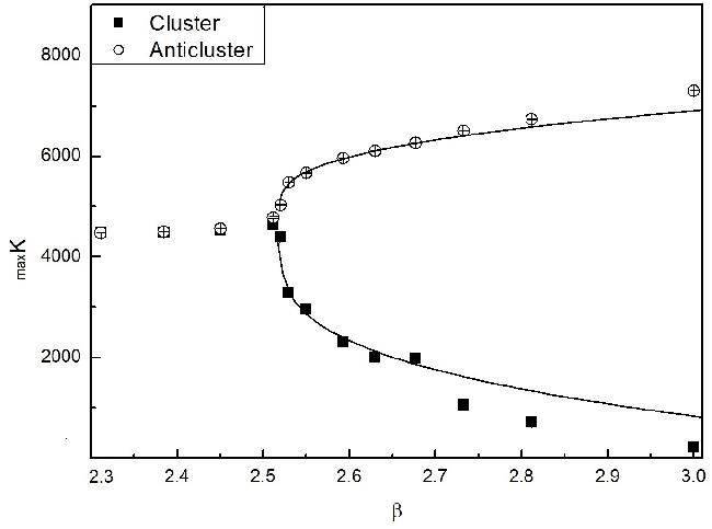
Figure 5.: Dependence of the mean size of the maximal (anti)cluster found for $L_{cut}=0.1$ (left panel) and for $L_{cut}=0.2$ (right panel). The curves represent Eq. (7).

Conclusions

In this contribution we present a novel approach to study the deconfinement PT in the SU(2) pure gauge theory in terms of the geometrical clusters composed of the Polyakov loops of the same sign. We demonstrate that the separation of (anti)clusters into “liquid” droplet and “gas” of smaller fragments is well justified and reflects the physical properties of the lattice system. This concept allows us to explain the deconfinement PT as a special kind of the liquid-gas transition. However, in contrast to the ordinary liquids, the SU(2) gluodynamics contains two types of liquid whose behavior is drastically different in the region of broken global Z(2) symmetry. The cluster liquid droplet evaporates above PT whereas the anticluster liquid droplet experiences the condensation of the accompanying gas of anticlusters. A successful application of the LDF to the description of the size distributions of gaseous (anti)clusters is the main result of this study. Surprisingly, even the monomers are qualitatively described by Eq. (2). The fit of the (anti)cluster size distributions by the LDF formula allows us to determine the $\beta$-dependences of the reduced chemical potential and the reduced surface tension coefficient. While in the symmetric phase this quantities are identical for fragments of both kinds, their behavior is drastically different in the deconfined phase. Another important finding of this study is a high precision determination of the Fisher topological constant $\tau=1.806\pm 0.008$ which is the same both for clusters and for anticlusters. This result is in line with the exactly solvable model of the nuclear liquid-gas PT [Sagun et al., 2014]. At the same time it disproves the FDM prediction that $\tau>2$ [Fisher, 1968]. We showed that the reduced surface tension coefficient and the mean size of the largest (anti)cluster can be used as the new order parameters of deconfinement PT in SU(2) gluodynamics. In contrast to the FDM the power law for the size distribution is found only for the gas of clusters and not at the PT point, but at $\beta=3$.

Acknowledgments. The authors thank D. B. Blaschke, O. A. Borisenko, V. Chelnokov, Ch. Gattringer, D. H. Rischke, L. M. Satarov, H. Satz and E. Shuryak for the fruitful discussions and valuable comments. The present work was supported in part by the National Academy of Sciences of Ukraine and by the NAS of Ukraine grant of GRID simulations for high energy physics.

References

L. G. Yaffe and B. Svetitsky, Phys. Rev. D, 26, 963, 1982.

L. G. Yaffe, and B. Svetitsky, Nucl. Phys. B, 210, 423, 1982.

S. Fortunato and H. Satz, Phys. Lett. B, 475, 311, 2000.

S. Fortunato et. al., Phys. Lett. B, 502, 321, 2001.

C. Gattringer, Phys. Lett. B, 690, 179 (2010).

C. Gattringer and A. Schmidt, JHEP 1101, 051, 2011.

M. E. Fisher, Physics, 3, 255, 1967.

M. E. Fisher, Rep. Prog. Phys., 30, 615, 1969.

J. Fingberg, U. Heller and F. Karsch, Nucl. Phys. B, 392, 493, 1993.

A.I. Ivanytskyi et al., arXive:1606.0471 [hep-lat].

V.Sagun, A.Ivanytskyi, K.Bugaev and I.Mishustin, Nucl.Phys. A, 924, 24, 2014.

M. Campostrini, A. Pelissetto, P. Rossi and E. Vicari, Phys. Rev. E, 65, 066127, 2002.

K. Huang, Statistical Mechanics, Wiley, New York, 1987.