MITP/16-110
TTP16-053
Massive three-loop form factor in the planar limit
Abstract
We compute the three-loop QCD corrections to the massive quark-anti-quark-photon form factors and in the large- limit. The analytic results are expressed in terms of Goncharov polylogarithms. This allows for a straightforward numerical evaluation. We also derive series expansions, including power suppressed terms, for three kinematic regions corresponding to small and large invariant masses of the photon momentum, and small velocities of the heavy quarks.
PACS numbers: 12.38.Bx, 12.38.Cy, 11.15.Bt, 14.65.Ha
1 Introduction
Massive form factors are important building blocks for various physical quantities involving heavy quarks. Among them are static quantities like anomalous magnetic moments but also production cross sections and decay rates. Furthermore, form factors are the prime examples for studying the infrared behaviour of QCD amplitudes.
We consider QCD corrections to the quark-photon vertex. The latter can be parametrized as follows,
| (1) |
where the colour indices of the quarks are suppressed and and are the spinors of the quark and anti-quark, respectively. The momentum is incoming and is outgoing with .
The vertex function can be decomposed into two scalar form factors which are usually introduced as
| (2) |
where is the outgoing momentum of the photon and . is the charge of the considered quark. and are often referred to as electric and magnetic form factors.


Sample Feynman diagrams can be found in Fig. 1. Two-loop QCD corrections to the electric and magnetic form factors for the heavy quark vector current have been computed for the first time in Ref. [1] (axial vector and anomaly contributions have been considered in [2, 3]) where analytic results have been obtained. An independent cross check of the two-loop results for and has been performed in [4] where also and terms have been added to the one- and two-loop results, respectively. The results have been used to obtain predictions for the three-loop form factor in the high energy limit, by exploiting evolution equations and the exponentiation of infrared divergences (see also Ref. [5] for earlier considerations).
In this paper we compute the three-loop form factor in the planar limit, keeping the exact mass dependence. After expanding our exact result for small quark masses we can compare to the high-energy results of [4] mentioned above, and complete them by determining the unknown constants in the and part. We furthermore provide power-suppressed terms.
Massive form factors have infrared divergences that are well understood. After the ultraviolet renormalization, all poles in dimensional regularization are given in terms of the cusp anomalous dimension [6, 7], and the beta function. The three-loop cusp anomalous dimension was computed in Ref. [8, 9]. By verifying the infrared pole structure at the three-loop order, we provide a first independent check of the result of Ref. [8, 9] (in the planar limit).
In the static limit, the infrared divergences disappear, and and are finite. In fact, vanishes and determines the anomalous magnetic moment of a heavy quark which has been considered at two-loop order in Ref. [10]. A dedicated calculation at three loops has been performed in Ref. [11] which serves as a welcome check for our exact result expanded for .
The remainder of the paper is organized as follows. In Section 2 we provide technical details on the calculation of the amplitudes. In particular we briefly describe the renormalization procedure. The infrared structure of the form factors is presented in Section 3. Our results for and are discussed in Section 4 including the three-loop results for the static limit, the high-energy limit and for small quark velocities. We conclude in Section 5.
2 Setup and calculation
The form factors and appearing in Eq. (2) are conveniently computed with the help of projectors which are applied to . Using the kinematics defined in Eq. (2) we have ()111Note that there is a typo in Eq. (11) of [1]: should read .
| (3) |
with
| (4) |
and . It is convenient to introduce the dimensionless variable
| (5) |
Then the low-energy, high-energy and threshold limits correspond to , and , respectively. Note that for we have and thus the form factors do not have imaginary parts. The same is true for with . For we have that is on the upper half of the unit circle.
It is convenient to write the perturbative expansion of () in the form
| (6) |
with and . In the large- limit we furthermore have that , , and , where counts the number of closed massless quark loops and is the number of colours. Note that we do not consider contributions with massive closed fermion loops. In Eq. (6) we suppress the scale dependence of and .
The calculations performed in this paper use the groundwork performed in Ref. [12] where all scalar integral families up to three loops, which are needed for the massive form factors and in the large- limit, have been classified and the corresponding master integrals have been computed analytically in terms of Goncharov polylogarithms [13]. We use in particular the information from Fig. 1 of Ref. [12] where eight three-loop families are defined. This information is used to generate with the help of the programs qgraf [14] and q2e/exp [15, 16] amplitudes for and which are expressed in terms of linear combinations of integrals from the eight three-loop families. We also use formulae for reduction of Goncharov polylogarithm values at sixth roots of unity derived in [17].
For the reduction to master integrals we use the program FIRE [18, 19, 20] in combination with LiteRed [21, 22]. Once the reduction for each family is complete we use the program tsort, which is part of the latest FIRE version [20] and based on ideas presented in Ref. [19], to obtain relations between primary master integrals, and to arrive at a minimal set. This leads to 89 master integrals needed for the large- limit of and .
In our calculation we allow for a general QCD gauge parameter but set terms ( corresponds to Feynman gauge) to zero before performing the reduction to master integrals. The bare form factors still contain linear terms which only drop out after renormalization. This serves as a welcome check for our calculation.
The ultraviolet renormalized form factors are obtained by renormalizing the strong counpling constant in the scheme and the heavy quark mass on-shell. Both counterterms are needed to two-loop accuracy and are well-known in the literature. Note, however, that for the on-shell mass counterterm higher order terms are needed. The latter can be found in Ref. [23].
In this context we would like to mention that in Ref. [1] an non-standard version of the scheme has been employed as can bee seen from Eq. (24) of that paper. The quantity , which enters the definition of the renormalization constant, induces terms which enter the part of the two-loop form factor. See also the discussion in Ref. [5] on this subject.
3 Infrared divergences of massive form factors
Form factors of massive particles have infrared divergences originating from exchanges of soft particles. The latter can be described in the eikonal approximation. In this way, the infrared divergences of the form factors can be mapped to ultraviolet divergences of Wilson lines [25]. The relevant Wilson line has the geometry of a cusp formed by the particle momenta. It obeys a renormalization group equation that is governed by the cusp anomalous dimension [6, 26, 7].
Applying this correspondence to the original form factors, one has
| (7) |
where is an infrared renormalization factor (in minimal subtraction), is the ultraviolet-renormalized form factor, and is finite both in the ultraviolet and infrared. In other words, all infrared poles of are reproduced by .
satisfies the following renormalization group equation
| (8) |
where is the renormalized strong coupling and is the -dimensional function,
| (9) |
with
| (10) |
Here and are the quadratic Casimir operators of the gauge group in the fundamental and adjoint representation, respectively, is the number of massless quark flavors, and .
The perturbative expansions of and have the form
| (11) |
Solving Eq. (8) to three loops, one finds
| (12) |
The cusp anomalous dimension in QCD was computed to three loops in [6, 7, 8, 9].
In this way, one can see explicitly the poles generated by the right-hand side of Eq. (7). We have verified that this equation correctly predicts all infrared poles in and to three loops.
4 Results
4.1 Structure of results for form factors
Before presenting explicit results we briefly discuss the general structure of our analytic expressions.
All relevant master integrals were computed analytically in Ref. [12]. From this it is clear that the form factors are given in terms of iterated integrals, with certain rational prefactors. The required set of integration kernels are
| (13) |
We sometimes refer to the arguments of the logarithms as letters.
Up to two-loop order and for the three-loop fermionic contributions (i.e. the and the terms) we observe only master integrals with letters and . This means that all of them can be expressed in terms of usual harmonic polylogarithms [27, 28].
On the other hand, the non-fermionic three-loop part has the additional letter . Introducing the complex roots of this polynomial, , one can write . In this way, all results can be written in terms of Goncharov polylogarithms. See Ref. [12] for more details.
At three-loop order we observe that plays a special role for the form factors and since the coefficients of the Goncharov polylogarithms develop poles up to sixth order in . We could show that these poles are artificial by expanding the Goncharov polylogarithms around . The analytic expressions for the finite result for and for are quite lengthy and can be found (for ) in the ancillary file.
4.2 Analytical results
We refrain from providing the results for the full three-loop form factors
since the analytic expressions are too lengthy.
All results which are discussed in this section can be downloaded
from https://www.ttp.kit.edu/preprints/2016/ttp16-053/.
It is instructive to consider the form factors and in various kinematical regions which have already been mentioned in the Introduction. They are discussed in the remaining part of this section. In Section 4.3 they are numerically compared to the exact result.
4.2.1 Low-energy: or
We start with the limit which we obtain by expanding the Goncharov polylogarithms in the master integrals for . The expansion has to be carried out carefully since there are higher order poles in in the prefactor. In fact, we expand all master integrals up to order and obtain and up to order . For the presentation in the paper we write and we restrict ourselves to expansion terms up to order , which for are given by
| (14) | |||||
Note that is finite and agrees with Eqs. (54) and (55) of Ref. [11] after adapting the large- limit.
4.2.2 High-energy: or
We expand all master integrals for up to order which is sufficient to obtain and up to order . For illustration we show the one-, two and three-loop results including the first power-suppressed corrections of order . It is convenient to write the -loop component of in the high-energy limit as follows
| (15) |
Our results for read (for )
| (16) | |||||
with . For we get the following expansion coefficients
| (17) | |||||
Note that the coefficients contain logarithmic terms in which leads to a divergent behaviour of for . For this reason we subtract when comparing with the exact result (cf Section 4.3). In Ref. [4] some of the pole parts for of the leading three-loop coefficient have been predicted using evolution equations. However, the term, the sub-leading terms of order with , and the results for are new (see also Subsection 4.4). Finally, we want to remark that higher order terms for the one- and two-loop coefficients can be found in the ancillary file.
4.2.3 Threshold: or
To obtain the threshold limit we expand the master integrals up to order . After inserting the expanded results into the expressions for the form factors it is convenient to use
| (18) |
where
| (19) |
is the velocity of the produced heavy quarks. Note that the ultravioletly renormalized form factors develop poles up to order where is the number of loops. On the other hand, the bare form factors have poles up to (cf. Ref. [4] where bare two-loop results are presented). Since the resulting expressions are quite large we refrain from displaying them in the paper but refer to the ancillary file which comes together with this paper. It is, however, instructive to look into the cross section , where is a heavy quark. Close to threshold it is determined by the virtual correction, i.e., the form factors and , since the contributions from real radiation are suppressed by a relative factor . In fact, we can write
| (20) | |||||
where . Our calculation of and determines the first three terms for each in the expansion for . Note that individually and still contain poles in , however, the combination given in Eq. (20) is finite. For the one-, two- and three-loop corrections we have
| (21) | |||||
where the ellipses refer to higher order terms in . The one- and two-loop expressions agree with the large- limit of Refs. [29, 30, 31] and the three-loop terms agree with Ref. [32, 33, 34].222We thank Andreas Maier for providing the result for in Eq. (A.6) of Ref. [34] and the corresponding two-loop expression in terms of Casimir invariants. At -loop order the leading term of behaves as which is determined by the Sommerfeld factor [35] with . It is interesting to note that the series expansion of has no term of order and thus starts at order which is confirmed by our explicit calculation.
In the context of effective theories an important quantity derived from the form factor is the matching coefficient between QCD and non-relativistic QCD of the vector current. It is obtained by considering the on-shell photon-quark vertex for . Due to the singularities in (see above) it is not possible to obtain the matching coefficient from the general result for . Rather a dedicated calculation is necessary which has been performed in [36] to three-loop order using semi-analytical methods. The planar master integrals of [36] have been computed in [12] as by-product of the calculation of all master integrals used in this calculation.
4.3 Numerical results
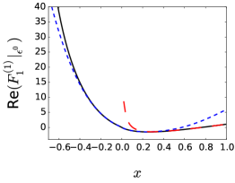
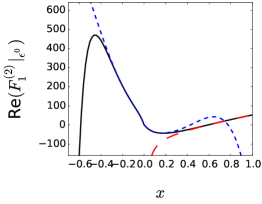
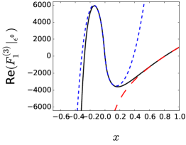
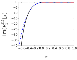
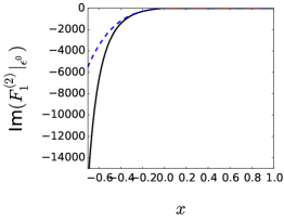
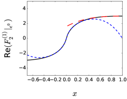
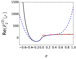
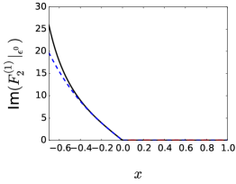
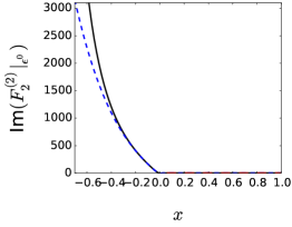
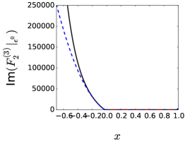
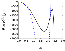
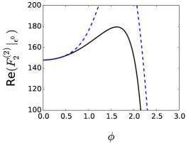
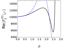
This subsection is devoted to the numerical evaluation of the form factors which we perform with the help of ginac [37, 38]. In Figs. 2 and 3 and are shown as a function of where the leading term of Eq. (15) is subtracted to obtain a regular behaviour for (which corresponds to ). From left to right the one-, two- and three-loop results are shown and the upper plots correspond to the real and the lower ones to the imaginary parts. Note that the latter are zero for . One observes that the expansions for (which include terms up to order ) provide a good approximation to the exact result in the interval which corresponds to . On the other hand, the approximations obtained for (which include terms up to order ) agree with the exact result for .
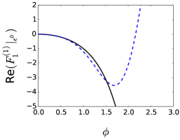
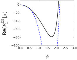
Fig. 4 shows the dependence of (top plots) and (bottom plots) as a function of where . In this region the form factors are real. One observes good agreement of the expanded and exact result up to which corresponds to .


4.4 Checks
Our result has passed several cross checks and consistency relations which we describe in this subsection.
We have successfully compared our bare and UV-renormalized one- and two-loop results (expanded up to ) to the expressions provided in Refs. [1, 4] after taking the large- limit. Note that in [1] a different renormalization scheme has been used which leads to a difference in the finite contribution proportional to . This is due to the factor which is present in the counterterm for the strong coupling constant in Eq. (24) of Ref. [1] (see also discussion above).
For the UV-renormalized two-loop form factor we agree with Ref. [4] including terms. For we disagree with the order term of Ref. [4] in a term which is independent of Goncharov polylogarithms. The difference of our result and the one of [4] reads
| (22) |
In our expression there is no term at all. Such a term leads to a different low-energy and threshold behaviour. In particular, the term of the renormalized two-loop form factor would have a stronger divergence than the expected behaviour, cf. the ancillary file to this paper. Furthermore, a term as in Eq. (22) influences via renormalization the terms of the three-loop which would lead to different low-energy and threshold expansions than the ones discussed in Section 4.2. In particular, would be different from zero and the agreement of in Eq. (21) with the literature would be destroyed.
As a further cross check we also compared with predictions of three-loop corrections to in the high-energy limit which have been obtained in Ref. [4] on the basis of evolution equations. We find agreement including the terms. The remaining and the terms cannot be predicted using the method of Ref. [4]. However, these terms are contained in our result.
From the pole of our result we can extract with the help of Eq. (12) the cusp anomalous dimension up to three-loop order in the large- limit. Up to two-loop order we find agreement with Refs. [7, 39] and at three loops we can reproduce the results of [8, 9]. This is the first independent check of (part of) the results obtained in [8, 9] using a completely different method.
We have checked that the renormalized form factors have the correct static limit. In particular, vanishes and agrees with the explicit calculation of the three-loop corrections to the anomalous magnetic moment of a heavy quark which was performed in Ref. [11].
For we have that . Thus the results for the form factors have to be real. Since the individual Goncharov polylogarithms are complex-valued this is a useful cross check.
Similarly, if with either or (i.e. is on the upper or lower semi-circle) we have that is below threshold with . Again, the form factors must be real-valued.
5 Conclusions and outlook
In this paper we evaluated for the first time massive three-loop form factors, in the planar limit. As a byproduct, we confirmed the recent result for the three-loop cusp anomalous dimension in the large- limit, which describes the infrared divergences of the form factors. We expressed the results analytically in terms of Goncharov polylogarithms. The latter allow for a straightforward numerical evaluation.
We investigated analytically the low-energy, threshold, and high-energy limits, and derived expressions containing logarithmically enhanced as well as power suppressed terms. It would be interesting if some of these expansions could be obtained from effective field theory methods. See for example Refs. [40, 41] for work on power-suppressed terms.
Acknowledgments
V.A.S. thanks Claude Duhr for help in manipulations with Goncharov polylogarithms and M.S. thanks Chihaya Anzai for support in the numerical evaluation of Goncharov polylogarithms. We thank Taushif Ahmed and Kirill Melnikov for useful discussions. This work is supported by the Deutsche Forschungsgemeinschaft through the project “Infrared and threshold effects in QCD”. J.M.H. thanks ICTP/SAIFR for hospitality during different stages of this work. J.M.H. is supported in part by a GFK fellowship and by the PRISMA cluster of excellence at Mainz university.
References
- [1] W. Bernreuther, R. Bonciani, T. Gehrmann, R. Heinesch, T. Leineweber, P. Mastrolia and E. Remiddi, Nucl. Phys. B 706 (2005) 245 doi:10.1016/j.nuclphysb.2004.10.059 [hep-ph/0406046].
- [2] W. Bernreuther, R. Bonciani, T. Gehrmann, R. Heinesch, T. Leineweber, P. Mastrolia and E. Remiddi, Nucl. Phys. B 712 (2005) 229 doi:10.1016/j.nuclphysb.2005.01.035 [hep-ph/0412259].
- [3] W. Bernreuther, R. Bonciani, T. Gehrmann, R. Heinesch, T. Leineweber and E. Remiddi, Nucl. Phys. B 723 (2005) 91 doi:10.1016/j.nuclphysb.2005.06.025 [hep-ph/0504190].
- [4] J. Gluza, A. Mitov, S. Moch and T. Riemann, JHEP 0907 (2009) 001 doi:10.1088/1126-6708/2009/07/001 [arXiv:0905.1137 [hep-ph]].
- [5] A. Mitov and S. Moch, JHEP 0705 (2007) 001 doi:10.1088/1126-6708/2007/05/001 [hep-ph/0612149].
- [6] A. M. Polyakov, Nucl. Phys. B 164 (1980) 171. doi:10.1016/0550-3213(80)90507-6
- [7] G. P. Korchemsky and A. V. Radyushkin, Nucl. Phys. B 283 (1987) 342. doi:10.1016/0550-3213(87)90277-X
- [8] A. Grozin, J. M. Henn, G. P. Korchemsky and P. Marquard, Phys. Rev. Lett. 114 (2015) no.6, 062006 doi:10.1103/PhysRevLett.114.062006 [arXiv:1409.0023 [hep-ph]].
- [9] A. Grozin, J. M. Henn, G. P. Korchemsky and P. Marquard, JHEP 1601 (2016) 140 doi:10.1007/JHEP01(2016)140 [arXiv:1510.07803 [hep-ph]].
- [10] W. Bernreuther, R. Bonciani, T. Gehrmann, R. Heinesch, T. Leineweber, P. Mastrolia and E. Remiddi, Phys. Rev. Lett. 95 (2005) 261802 doi:10.1103/PhysRevLett.95.261802 [hep-ph/0509341].
- [11] A. G. Grozin, P. Marquard, J. H. Piclum and M. Steinhauser, Nucl. Phys. B 789 (2008) 277 doi:10.1016/j.nuclphysb.2007.08.012 [arXiv:0707.1388 [hep-ph]].
- [12] J. M. Henn, A. V. Smirnov and V. A. Smirnov, arXiv:1611.06523 [hep-ph].
- [13] A. B. Goncharov, Math. Res. Lett. 5 (1998) 497 doi:10.4310/MRL.1998.v5.n4.a7 [arXiv:1105.2076 [math.AG]].
- [14] P. Nogueira, J. Comput. Phys. 105 (1993) 279.
- [15] R. Harlander, T. Seidensticker and M. Steinhauser, Phys. Lett. B 426 (1998) 125 [hep-ph/9712228].
- [16] T. Seidensticker, hep-ph/9905298.
- [17] J. M. Henn, A. V. Smirnov and V. A. Smirnov, arXiv:1512.08389 [hep-th].
- [18] A. V. Smirnov, JHEP 0810 (2008) 107 doi:10.1088/1126-6708/2008/10/107 [arXiv:0807.3243 [hep-ph]].
- [19] A. V. Smirnov and V. A. Smirnov, Comput. Phys. Commun. 184 (2013) 2820 doi:10.1016/j.cpc.2013.06.016 [arXiv:1302.5885 [hep-ph]].
- [20] A. V. Smirnov, Comput. Phys. Commun. 189 (2015) 182 doi:10.1016/j.cpc.2014.11.024 [arXiv:1408.2372 [hep-ph]].
- [21] R. N. Lee, arXiv:1212.2685 [hep-ph].
- [22] R. N. Lee, J. Phys. Conf. Ser. 523 (2014) 012059 doi:10.1088/1742-6596/523/1/012059 [arXiv:1310.1145 [hep-ph]].
- [23] P. Marquard, L. Mihaila, J. H. Piclum and M. Steinhauser, Nucl. Phys. B 773 (2007) 1 doi:10.1016/j.nuclphysb.2007.03.010 [hep-ph/0702185].
- [24] K. Melnikov and T. van Ritbergen, Nucl. Phys. B 591 (2000) 515 doi:10.1016/S0550-3213(00)00526-5 [hep-ph/0005131].
- [25] G. P. Korchemsky and A. V. Radyushkin, Phys. Lett. B 279 (1992) 359 doi:10.1016/0370-2693(92)90405-S [hep-ph/9203222].
- [26] R. A. Brandt, F. Neri and M. a. Sato, Phys. Rev. D 24 (1981) 879. doi:10.1103/PhysRevD.24.879
- [27] E. Remiddi and J. A. M. Vermaseren, Int. J. Mod. Phys. A 15 (2000) 725 doi:10.1142/S0217751X00000367 [hep-ph/9905237].
- [28] D. Maitre, Comput. Phys. Commun. 174 (2006) 222 [arXiv:hep-ph/0507152].
- [29] A. O. G. Kallen and A. Sabry, Kong. Dan. Vid. Sel. Mat. Fys. Med. 29 (1955) no.17, 1.
- [30] A. Czarnecki and K. Melnikov, Phys. Rev. Lett. 80 (1998) 2531 doi:10.1103/PhysRevLett.80.2531 [hep-ph/9712222].
- [31] M. Beneke, A. Signer and V. A. Smirnov, Phys. Rev. Lett. 80 (1998) 2535 doi:10.1103/PhysRevLett.80.2535 [hep-ph/9712302].
- [32] A. Pineda and A. Signer, Nucl. Phys. B 762 (2007) 67 doi:10.1016/j.nuclphysb.2006.09.025 [hep-ph/0607239].
- [33] A. H. Hoang, V. Mateu and S. Mohammad Zebarjad, Nucl. Phys. B 813 (2009) 349 doi:10.1016/j.nuclphysb.2008.12.005 [arXiv:0807.4173 [hep-ph]].
- [34] Y. Kiyo, A. Maier, P. Maierhofer and P. Marquard, Nucl. Phys. B 823 (2009) 269 doi:10.1016/j.nuclphysb.2009.08.010 [arXiv:0907.2120 [hep-ph]].
- [35] See, e.g., A. Messiah, “Quantum Mechanics Volume II”, North Holland.
- [36] P. Marquard, J. H. Piclum, D. Seidel and M. Steinhauser, Phys. Rev. D 89 (2014) no.3, 034027 doi:10.1103/PhysRevD.89.034027 [arXiv:1401.3004 [hep-ph]].
- [37] C. W. Bauer, A. Frink and R. Kreckel, J. Symb. Comput. 33 (2000) 1 [cs/0004015 [cs-sc]].
- [38] J. Vollinga and S. Weinzierl, Comput. Phys. Commun. 167 (2005) 177 doi:10.1016/j.cpc.2004.12.009 [hep-ph/0410259].
- [39] N. Kidonakis, Phys. Rev. Lett. 102 (2009) 232003 doi:10.1103/PhysRevLett.102.232003 [arXiv:0903.2561 [hep-ph]].
- [40] E. Laenen, L. Magnea, G. Stavenga and C. D. White, JHEP 1101, 141 (2011) doi:10.1007/JHEP01(2011)141 [arXiv:1010.1860 [hep-ph]].
- [41] A. A. Penin and N. Zerf, Phys. Lett. B 760, 816 (2016) doi:10.1016/j.physletb.2016.07.077 [arXiv:1606.06344 [hep-ph]].